Strong order of convergence of a semidiscrete scheme for the stochastic Manakov equation

Abstract

It is well accepted by physicists that the Manakov PMD equation is a good model to describe the evolution of nonlinear electric fields in optical fibers with randomly varying birefringence. In the regime of the diffusion approximation theory, an effective asymptotic dynamics has recently been obtained to describe this evolution. This equation is called the stochastic Manakov equation. In this article, we propose a semidiscrete version of a Crank Nicolson scheme for this limit equation and we analyze the strong error. Allowing sufficient regularity of the initial data, we prove that the numerical scheme has strong order $1/2$.

Keywords : Stochastic partial differential equations, Numerical schemes, Rate of convergence, System of coupled nonlinear Schrödinger equations, Polarization Mode Dispersion.

MSC2010 subject classifications : 60H15, 35Q55, 60M15.

1 Introduction

The development of Internet and of the Web, in the second half of the $20^{e}$ century, has allowed for a rapid progress of optical communication systems. Today, engineers and physicists are trying to rise the bandwidths capacity of these communication systems as the Internet traffic has increased the last few years. However, some dispersive effects limit the rate of transmission of information. The Polarization Mode Dispersion (PMD), appearing when the two components of the electric field do not travel with the same characteristics, is one of the limiting factors of high bit rate transmissions. The Manakov PMD equation was derived from the Maxwell equations to study light propagation over long distances in such optical fibers [32]. Due to the various length scales present in this problem, a small parameter $\epsilon$ appears in the rescaled equation. Using separation of scales techniques, the author proved in [6, 13] that the asymptotic dynamics is described by a stochastic perturbation, in the stratonovich sense, of the Manakov equation. In this article, we consider a semidiscrete version of a Crank Nicolson scheme for the stochastic Manakov equation. Our aim is to analyze the order of the error for this scheme and we prove that the strong order is $1/2$.

Numerical simulations are used in practice to solve complicated stochastic differential equations and to lighten some hidden behaviours such as large deviations. In optics, numerical simulations of the stochastic Manakov equation may help to understand the impact of the Polarization Mode Dispersion (PMD) on the pulse spreading [14]. Depending on the problem, one may not be interested in the same quantities. On one hand, one may be interested in the computation of path samples (related to strong solutions) to emphasize, for example, the relation between various parameters in the dynamics. On the other hand, if the quantity under interest depends only on the law of the dynamics, one will focus on weak approximations. The pathwise error analysis of numerical schemes for SDE has been intensively studied [12, 21, 26, 30], whereas the weak error analysis started later with the work of Milstein [24, 25] and Talay [31], who used the Kolmogorov equation associated to the SDE to obtain a weak order of convergence. Usually, for Euler schemes, the strong order is $1/2$. More sophisticated schemes exist to increase the pathwise order but their numerical implementation requires to compute multiple iterated integrals, which may be difficult if the dynamics is driven by a multi-dimensional Brownian motion.

The numerical analysis of SPDEs combines stochastic analysis together with PDEs numerical approximation. Most of the results are concerned with the analysis of pathwise convergence for solutions of semi-linear and quasi-linear parabolic equations (for a non exhaustive list, see [2, 15, 16, 17, 19, 23, 28]). There is some recent literature on dispersive equations, both for stochastic nonlinear Schrödinger equations [4, 5, 22] and for a stochastic Korteweg-de-Vries equation [8, 9]. Weak order for SPDEs has been considered later [7, 10, 20]; the proof consists then in using the Kolmogorov equation which is now a PDE with an infinite number of variables.

In our case, the difficult and innovative point lies in the linear estimate. Indeed, the noise term contains a one order derivative and hence cannot be treated as a perturbation [6, 13]. Moreover an implicit discretization of the noise has to be considered to build a conservative scheme and the delicate point, in order to obtain the strong error, is to deal with random matrices. Indeed, the linear system to be solved contains random coefficients and the expression of the global error contains terms that are not martingales. Hence, the usual arguments consisting of applying the Burkholder-Davis-Gundy inequality to the stochastic integral cannot be applied straightforwardly. The probability order for the nonlinear scheme is obtained using classical arguments [5, 28]. This notion is not usual in the context of numerical analysis of stochastic equation. It is weaker than the strong order in time and is used here because of the nonlinear drift.

In this article, we consider the order of convergence of a semi-discrete scheme. For smooth initial data, it is probable that the error analysis of the fully discrete scheme is not a problem and that the strong order in space is the same as in the deterministic case.

1.1 Presentation of the numerical scheme

The stochastic Manakov equation is given by

$$idX(t)+\left(\frac{\partial^{2}X(t)}{\partial x^{2}}+F\left(X(t)\right)\right)dt+i\sqrt{\gamma}\sum_{k=1}^{3}\sigma_{k}\frac{\partial X(t)}{\partial x}\circ dW_{k}(t)=0,\quad t\geqslant 0,x\in\mathds{R}$$ (1.1)

where the $\mathds{C}^{2}$ vector of unknown $X=(X_{1},X_{2})$ is a random process on a probability space $(\Omega,\mathcal{F},\mathds{P})$, $\gamma$ is a small positive parameter given by the physics of the problem, $W=(W_{1},W_{2},W_{3})$ is a $3$-dimensional Brownian motion and $\circ$ denotes the Stratonovich product. The matrices $\sigma_{1},\sigma_{2},\sigma_{3}$ are the Pauli matrices

$$\sigma_{1}=\begin{pmatrix}0&1\\ 1&0\\ \end{pmatrix},\;\;\sigma_{2}=\begin{pmatrix}0&-i\\ i&0\\ \end{pmatrix},\;\;\sigma_{3}=\begin{pmatrix}1&0\\ 0&-1\\ \end{pmatrix},$$

and the nonlinear term is given by $F\left(X(t)\right)=\left|X\right|^{2}X(t)$. The equivalent Itô formulation is given by

$$dX(t)=\left(C_{\gamma}\frac{\partial^{2}X(t)}{\partial x^{2}}+iF{\left(X\right)}(t)\right)dt-\sqrt{\gamma}\sum_{k=1}^{3}\sigma_{k}\frac{\partial X(t)}{\partial x}dW_{k}(t).$$ (1.2)

where $C_{\gamma}=i+\frac{3\gamma}{2}$. In the deterministic case (i.e. when $\gamma=0$), when one considers the Manakov Equation, both the mass (equal to the $\mathds{L}^{2}$ norm) and the Hamiltonian $H$ given by

$$H(X)=\frac{1}{2}\int_{\mathds{R}}\left|\frac{\partial X}{\partial x}\right|^{2}dx-\frac{1}{4}\int_{\mathds{R}}\left|X\right|^{4}dx$$

are conserved as time varies. This is not the case for the stochastic Manakov equation that preserves only the mass, the Hamiltonian structure being destroyed by the noise [6, 13]. Several numerical approximations have been proposed to simulate the solution of the deterministic equation, such as the Crank-Nicolson scheme [11], the relaxation scheme [1] and Fourier split-step schemes [29, 33]. These schemes are known to be conservative for the $\mathds{L}^{2}$ norm. The time centering method, used to discretize the second order differential operator in the CN and relaxation schemes, allows them to be conservative for a discrete Hamiltonian. On the contrary, the splitting scheme fails in preserving exactly $H$.

The question that needs to be addressed is the discretization of the noise term. There are actually two different approaches based on the fact that, in the continuous case, Equation (1.1) and Equation (1.2) are equivalent. Hence, one may either propose a semi-implicit discretization of the Stratonovich integral, using the midpoint rule, or an explicit discretization of the Itô integral. However, in the discrete setting, the two formulations are not equivalent. Indeed, the discrete $\mathds{L}^{2}$ norm is not preserved when considering an Euler scheme based on the Itô equation, while the semi-implicit discretization of the Stratonovich integral allows preservation of the mass. Note that the conservation of the discrete mass immediately leads to the unconditional $\mathds{L}^{2}$ stability of the scheme.

There is actually a more profound reason that keeps us from using a numerical scheme based on the Itô equation; this reason lies in the fact that the noise term contains a one order derivative. It is well known from the deterministic literature, that explicit schemes for the advection equation require a stability criterion (CFL condition) to converge, while implicit schemes are stable. When considering the Itô approach, the discretization of the stochastic integral has to be explicit in order to be consistent with the equation, since an implicit discretization converges to the backward Itô integral. Therefore, the Itô approach leads to a CFL condition that depends on Gaussian random variables. Since they are not bounded, this random stability condition may be very restrictive.

We consider a semi-discrete Crank-Nicolson scheme given by

$$\left\{\begin{array}[]{ll}X^{n+1}_{N}-X^{n}_{N}+H_{\Delta t,n}X^{n+1/2}_{N}-iF\left(X^{n}_{N},X^{n+1}_{N}\right)\Delta t=0\\[5.69046pt] F\left(X^{n}_{N},X^{n+1}_{N}\right)=\frac{1}{2}\left(\left|X^{n}_{N}\right|^{2}+\left|X^{n+1}_{N}\right|^{2}\right)X^{n+1/2}_{N},\end{array}\right.$$ (1.5)

where $X^{n+1/2}_{N}=\left(X^{n+1}_{N}+X^{n}_{N}\right)/2$, the time step is denoted $\Delta t$ and $\sqrt{\Delta t}\chi_{k}^{n}=W_{k}\left((n+1)\Delta t\right)-W_{k}\left(n\Delta t\right),k=1,2,3$ is the noise increment. The random matrix operator $H_{\Delta t,n}$ is defined by

$$H_{\Delta t,n}=-i\Delta tI_{2}\partial_{x}^{2}+\sqrt{\gamma\Delta t}\sum_{k=1}^{3}\sigma_{k}\chi_{k}^{n}\partial_{x}.$$ (1.6)

with domain $\mathscr{D}(H_{\Delta t,n})=\mathds{H}^{2}\left(\mathds{R}\right)\subset\mathds{L}^{2}\left(\mathds{R}\right)$ independent of $n$, where $\mathds{H}^{2}\left(\mathds{R}\right)$ is the space of functions in $\mathds{L}^{2}$ such that their first two derivatives are in $\mathds{L}^{2}$. The $2\times 2$ identity matrix is denoted by $I_{2}$.

This paper is organized as follows. In section 1.2, we introduce some notations and the main result of this article. Then, following the approach of [6, 13] for the continuous equation, we construct a discrete random propagator associated to the linear equation. In section 2, we study the linear Euler scheme with semi-implicit discretization of the noise and prove that the strong order is $1/2$. In section 3, we give a result on the strong order of convergence for a nonlinear equation with globally Lipschitz nonlinear terms. From this result and following the arguments of [5], we obtain that the order of convergence in probability and the almost sure order are $1/2$. This theoretical result is numerically recovered in section 4 where almost sure convergence curves are displayed. Finally some technical results are proved in section 5.

1.2 Notation and main result

For all $p\geqslant 1$, we define $\mathds{L}^{p}(\mathds{R})=\left(L^{p}(\mathds{R};\mathds{C})\right)^{2}$ the Lebesgue spaces of functions with values in $\mathds{C}^{2}$. Identifying $\mathds{C}$ with $\mathds{R}^{2}$, we define a scalar product on $\mathds{L}^{2}\left(\mathds{R}\right)$ by

$$\left(u,v\right)_{\mathds{L}^{2}}=\sum_{i=1}^{2}\mathcal{R}\mbox{e}\left\{\int_{\mathds{R}}u_{i}\overline{v_{i}}dx\right\}.$$

We denote by $\mathds{H}^{m}\left(\mathds{R}\right),m\in\mathds{N}$ the space of functions in $\mathds{L}^{2}$ such that their $m$ first derivatives are in $\mathds{L}^{2}$. We will also use $\mathds{H}^{-m}$ the topological dual space of $\mathds{H}^{m}$ and denote $\left<.,.\right>$ the paring between $\mathds{H}^{m}$ and $\mathds{H}^{-m}$. The Fourier transform of a tempered distribution $v\in\mathcal{S}^{\prime}(\mathds{R})$ is either denoted by $\widehat{v}$ or $\mathcal{F}v$. If $s\in\mathds{R}$ then $\mathds{H}^{s}$ is the fractional Sobolev space of tempered distributions $v\in\mathcal{S}^{\prime}(\mathds{R})$ such that $(1+\left|\xi\right|^{2})^{s/2}\widehat{v}\in\mathds{L}^{2}$. Let $\left(E,\left\|.\right\|_{E}\right)$ and $\left(F,\left\|.\right\|_{F}\right)$ be two Banach spaces. We denote by $\mathcal{L}\left(E,F\right)$ the space of linear continuous functions from $E$ into $F$, endowed with its natural norm. If $I$ is an interval of $\mathds{R}$ and $1\leqslant p\leqslant+\infty$, then $L^{p}\left(I;E\right)$ is the space of strongly Lebesgue measurable functions $f$ from $I$ into $E$ such that $t\mapsto\left\|f(t)\right\|_{E}$ is in $L^{p}(I)$. The space $L^{p}\left(\Omega,E\right)$ is defined similarly where $\left(\Omega,\mathcal{F},\mathds{P}\right)$ is a probability space.

We now recall some results obtained in [6, 13] on the existence of a solution for the system (1.1). Let $\left(\Omega,\mathcal{F},\mathds{P}\right)$ be a probability space on which is defined a $3$-dimensional Brownian motion $W(t)=\left(W_{k}(t)\right)_{k=1,2,3}$. We endow this space with the complete filtration $\mathcal{F}_{t}$ generated by $W(t)$. The local existence result obtained for (1.1) is stated below.

Theorem 1.1.

Let $X_{0}=v\in\mathds{H}^{1}(\mathds{R})$ then there exists a maximal stopping time $\tau^{*}(v,\omega)$ and a unique strong adapted solution $X$ (in the probabilistic sense) to (1.1), such that $X\in C\left([0,\tau^{*}),\mathds{H}^{1}\left(\mathds{R}\right)\right)$ $\mathds{P}-a.s$. Furthermore the $\mathds{L}^{2}$ norm is almost surely preserved, i.e, $\forall t\in[0,\tau^{*}),\left\|X(t)\right\|_{\mathds{L}^{2}}=\left\|v\right\|_{\mathds{L}^{2}}$ and the following alternative holds for the maximal existence time of the solution :

$$\tau^{*}(v,\omega)=+\infty\ \text{ or }\ \limsup\limits_{t\nearrow\tau^{*}(v,\omega)}\left\|X(t)\right\|_{\mathds{H}^{1}}=+\infty.$$

Moreover if the initial data $X_{0}$ belongs to $\mathds{H}^{m},m\geqslant 1$, then the corresponding solution belongs to $\mathds{H}^{m}$.

The noise ($\gamma\neq 0$ in Equation (1.1)) destroys the Hamiltonian structure of the deterministic equation and it seems that no control on the evolution of the $\mathds{H}^{1}$ norm is available from the evolution of the energy. However, the occurrence of blow up in this model remains an open question. We assume that the set $\left\{\Delta t\right\}=\left\{\Delta t_{n}\right\}_{n\in\mathds{N}}$ is a discrete sequence converging to $0$. We define a final time $T>0$ and an interval $[0,T]$ on which we will consider the approximation of the solution of (1.1). Moreover $N_{T}=[T/\Delta t]$, the integer part of $T/\Delta t$. Similarly for any stopping time $\tau$, $N_{\tau}=[\tau/\Delta t]$. Moreover we write $t_{n}=n\Delta t$ for any $n\in[\![0,N]\!]$ where $N$ is either $N_{T}$ or $N_{\tau}$ according to the situation. We denote by $L^{\infty}\left(0,T;\mathds{H}^{m}\right)$ the space of all bounded sequences for $n=0,\cdots,N_{T}$ with values in $\mathds{H}^{m}$ endowed with the supremum norm

$$\left\|X_{N}\right\|_{L^{\infty}\left(0,T;\mathds{H}^{m}\right)}=\underset{n\Delta t\leqslant T}{\sup_{n\in\mathds{N}}}\left\|X^{n}_{N}\right\|_{\mathds{H}^{m}}.$$

Moreover for a $n\times n$ matrix $A=\left\{a_{ij}\right\}$, the uniform norm is defined by

$$\left\|\left|A\right|\right\|_{\infty}=\max_{1\leqslant i\leqslant n}\sum_{j=1}^{n}\left|a_{ij}\right|$$

and the spectral norm of $A$ is defined by

$$\left\|\left|A\right|\right\|_{2}=\sqrt{\rho\left(A^{*}A\right)}$$

where $A^{*}$ is the adjoint matrix of $A$ and $\rho$ is the spectral radius. Finally we denote $dW_{0}(u)=du$ and we introduce the notations for $j,k\in\llbracket 0,3\rrbracket$

$$W^{n,s}_{j}\left(f\right)=\int_{t_{n}}^{s}f(u)dW_{j}(u)$$

$$W^{n,n+1}_{j,k}\left(f\right)=\int_{t_{n}}^{t_{n+1}}\int_{t_{n}}^{s}f(u)dW_{j}(u)dW_{k}(s).$$

We recall that the Pauli matrices have the following properties

Property 1.1.

Let $j,k,l\in\llbracket 0,3\rrbracket$, then

• Commutation relations : $\left[\sigma_{j},\sigma_{k}\right]=2i\sum_{l=1}^{3}\varepsilon_{jkl}\sigma_{l}$.

• Anticommutation relations : $\sigma_{j}\sigma_{k}+\sigma_{k}\sigma_{j}=2\delta_{jk}\cdot I_{2}$ and $\sigma_{j}=\sigma_{j}^{*}$,

where $\varepsilon_{jkl}=(j-k)(k-l)(l-j)/2$ is the Levi-Civita symbol.

We denote by $\widetilde{X}^{n}=X\left(t_{n}\right)$ the solution of Equation (1.1), evaluated at the point $t_{n}$. Let us now give the main result of this paper stating that the approximation of Equation (1.1) by the scheme (1.5) has an order $1/2$ in probability.

Theorem 1.2.

Assume that $X_{0}\in\mathds{H}^{6}$, then for any stopping time $\tau<\tau^{*}\wedge T$ almost surely we have

$$\lim_{C\to+\infty}\mathds{P}\left(\max_{n=0,\ldots,N_{\tau}}\left\|X^{n}-\widetilde{X}^{n}\right\|_{\mathds{H}^{1}}\geqslant C\Delta t^{1/2}\right)=0,$$

uniformly in $\Delta t$. Then we say, according to [28], that the scheme has an order $1/2$ in probability. Moreover, for any $\delta<\frac{1}{2}$, there exists a random variable $K_{\delta}$ such that

$$\max_{n=0,\ldots,N_{\tau}}\left\|X^{n}-\widetilde{X}^{n}\right\|_{\mathds{H}^{1}}\leqslant K_{\delta}(T,\omega)\Delta t^{\delta}.$$

2 The linear equation.

In this section, we study the approximation of the solution of the linear equation. In other words, we estimate the error between the solution of

$$idX(t)+\frac{\partial^{2}X(t)}{\partial x^{2}}dt+i\sqrt{\gamma}\sum_{k=1}^{3}\sigma_{k}\frac{\partial X(t)}{\partial x}\circ dW_{k}(t)=0,\quad t\geqslant 0,x\in\mathds{R}$$ (2.1)

and its approximation by the semidiscrete mid-point scheme

$$X^{n+1}_{N}-X^{n}_{N}+H_{\Delta t,n}X^{n+1/2}_{N}=0,$$ (2.2)

where the expression of $H_{\Delta t,n}$ is given in (1.6). The operator $H_{\Delta t,n}$ is easily described thanks to the Fourier transform. Indeed, for any $\xi\in\mathds{R}$

$$\mathcal{F}\left(H_{\Delta t,n}\left(\xi\right)X\right)=\displaystyle{\begin{pmatrix}i\Delta t\left|\xi\right|^{2}+i\sqrt{\gamma\Delta t}\chi_{3}^{n}\xi&i\sqrt{\gamma\Delta t}\left(\chi_{1}^{n}-i\chi_{2}^{n}\right)\xi\\[5.69046pt] i\sqrt{\gamma\Delta t}\left(\chi_{1}^{n}+i\chi_{2}^{n}\right)\xi&i\Delta t\left|\xi\right|^{2}-i\sqrt{\gamma\Delta t}\chi_{3}^{n}\xi\end{pmatrix}}\widehat{X}.$$ (2.3)

Moreover, we set

$$T_{\Delta t,n}=(\text{I\footnotesize{d}}+\frac{1}{2}H_{\Delta t,n}),$$ (2.4)

where Id is the identity mapping in $\mathds{L}^{2}$. To lighten the notation, we do not write the dependence in $N$ of the unknown $X_{N}$. The aim of this section is to give an existence result of an adapted solution for the scheme (2.2) and to give an estimate of the discretization error. The results are stated in Propositions 2.1 and 2.2 below.

2.1 Existence and stability

The next proposition states that the solution of the scheme (2.2) is uniquely defined and adapted, and that the mass is preserved.

Proposition 2.1.

Given $X_{0}\in\mathds{H}^{m}$ for $m\in\mathds{N}$, there exists a unique adapted discrete solution $\left(X^{n}\right)_{n=0,\cdots,N_{T}}$ to (2.2) that belongs to $L^{\infty}(0,T;\mathds{H}^{m})$. Moreover the $\mathds{H}^{m}$ norm of the solution $X^{n}$ of (2.2) is constant i.e. for all $n\in\llbracket 0,N_{T}\rrbracket$

$$\left\|X^{n}\right\|_{\mathds{H}^{m}}=\left\|X_{0}\right\|_{\mathds{H}^{m}}.$$ (2.5)

Proof of Proposition 2.1.

Assume that $X^{n}$ is a $\mathcal{F}_{n\Delta t}-$measurable random variable with values in $\mathds{H}^{m}$. We set $A_{\Delta t}=\Delta tI_{2}\partial_{x}^{2}$ and $B_{\Delta t,n}=i\sqrt{\gamma\Delta t}\sum_{k=1}^{3}\sigma_{k}\chi_{k}^{n}\partial_{x}$, for a.e. $\omega\in\Omega$. Using Property 1.1 of the Pauli matrices, Cauchy-Schwarz and Young inequalities, we may prove that a.s.

$$\left\|B_{\Delta t,n}v\right\|_{\mathds{L}^{2}}^{2}\leqslant\frac{1}{2}\left\|A_{\Delta t,n}v\right\|_{\mathds{L}^{2}}^{2}+\frac{C(\gamma,\omega)^{2}}{2}\left\|v\right\|_{\mathds{L}^{2}}^{2},$$

where $C(\gamma,\omega)=3\gamma\left(\chi_{k}^{n}(\omega)\right)^{2}$. Since $\left|C(\gamma,\omega)\right|<+\infty\ \text{a.s.}$, we deduce thanks to the Kato-Rellich Theorem that $iH_{\Delta t,n}$ is selfadjoint in $\mathds{L}^{2}$ with domain $\mathds{H}^{2}$ and it follows that $T_{\Delta t,n}$ is invertible from $\mathds{H}^{2}$ into $\mathds{L}^{2}$. Hence, the unique $\mathcal{F}_{t_{n+1}}$– measurable solution is given by $X^{n+1}=U_{\Delta t,n}X^{n}$ a.s, where

$$U_{\Delta t,n}=(\text{I\footnotesize{d}}+\frac{1}{2}H_{\Delta t,n})^{-1}(\text{I\footnotesize{d}}-\frac{1}{2}H_{\Delta t,n}).$$ (2.6)

The conservation of the $\mathds{L}^{2}$ norm follows because $H_{\Delta t,n}$ is skew symmetric and $U_{\Delta t,n}^{*}U_{\Delta t,n}=\text{I\footnotesize{d}}$. ∎

Remark 2.1.

In our case, the operator $T_{\Delta t,n}$ is invertible for every $\Delta t$. Thus, the implementation of the scheme (2.2) does not require to use a truncation of the noise term as in [27] to insure stability.

2.2 Strong order of convergence

Let us now consider the order of convergence of the Crank Nicolson scheme (2.2). To this purpose, we denote by $\widetilde{X}^{n}=X\left(t_{n}\right)$ the solution of (2.1), evaluated at the point $t_{n}$, and define the vector error $e^{n}=\widetilde{X}^{n}-X^{n}$. The error estimates is given in the next result.

Proposition 2.2.

If $X_{0}\in\mathds{H}^{m+5}$, $m\in\mathds{N}$, then the scheme (2.2) is convergent and for any $p\geqslant 1$

$$\mathds{E}\left(\max_{n\in\llbracket 0,N_{T}\rrbracket}\left\|e^{n}\right\|_{\mathds{H}^{m}}^{2p}\right)\leqslant C(T,\gamma,p,\left\|X_{0}\right\|_{\mathds{H}^{m+5}})\Delta t^{p}.$$ (2.7)

It may be surprising to require so much regularity on the initial data to prove a $L^{p}(\Omega)$ order for a linear equation. Usually, the order is obtained using the explicit expression of the group $S(t)$, solution of the free Schrödinger equation (that is $\gamma=0$ in Equation (2.1)), and the mild form of the Itô equation. In our case, we cannot proceed similarly because of the semi-implicit discretization of the noise and the presence of a differential operator in this term.

Proof of Proposition 2.2.

Without loss of generality, we assume that $m=0$. The proof is divided into the following steps.

1. Firstly, we evaluate the growth of the solution of the continuous equation (2.1). More precisely, we denote by $\widetilde{e}^{\,n}(s)$ the difference $\widetilde{e}^{\,n}(s)=X(s)-\widetilde{X}^{n}$, for all $s\in[t_{n},t_{n+1}]$ and we give an estimate of it in the space $L^{2p}\left(\Omega,L^{\infty}\left(0,T;\mathds{L}^{2}\right)\right)$.

2. Secondly, we write a discrete Duhamel equation for the global error $e^{n}=X^{n}-\widetilde{X}^{n}$, where the Itô formulation of equation (2.1) is used.

3. The expression of the global error contains terms that are not martingales and hence martingales inequalities cannot be applied straightforwardly. Therefore, we separate the adapted part to the non adapted one introducing a discrete random propagator $\mathcal{V}^{l}_{\Delta t}$. The adapted part is estimated thanks to the usual martingale inequalities, while a bound on the non-adapted part is obtained estimating the difference between $\mathcal{V}^{l}_{\Delta t}$ and the discrete random propagator appearing in the expression of the global error.

Step 1.

The next lemma gives an estimate of the growth of the solution $X(s)$ of (2.1) starting at $\widetilde{X}^{n}$.

Lemma 2.1.

For any $p\geqslant 1$, if $X_{0}\in\mathds{H}^{1}$ then

$$\mathds{E}\left(\sup_{t_{n}\leqslant s\leqslant t_{n+1}}\left\|\widetilde{e}^{\,n}(s)\right\|_{\mathds{L}^{2}}^{2p}\right)\leqslant C_{p}(\gamma)\left\|X_{0}\right\|_{\mathds{H}^{1}}^{2p}\Delta t^{p}\qquad\forall n=0,\cdots,N_{T}-1.$$

Proof.

Writing the Itô formulation of Equation (2.1) under its mild form, we get

$$X(t)-\widetilde{X}^{n}=\left(S(t-t_{n})-\text{I\footnotesize{d}}\right)\widetilde{X}^{n}+i\sqrt{\gamma}\sum_{k=1}^{3}\int_{t_{n}}^{t}S(t-u)\sigma_{k}\partial_{x}X(u)dW_{k}(u),$$

where $S(t)$ is the semi-group solution of the linear equation $\partial_{t}X(t)=C_{\gamma}\partial_{x}^{2}X(t)$ with $C_{\gamma}=i+\frac{3\gamma}{2}$. Using the Fourier transform, it can easily be shown that

$$\left\|\left(S(t)-\text{I\footnotesize{d}}\right)f\right\|_{\mathds{L}^{2}}\leqslant C(\gamma)t^{1/2}\left\|f\right\|_{\mathds{H}^{1}},\qquad\forall f\in\mathds{H}^{1},$$

from which we deduce, together with (2.5), that

$$\mathds{E}\left(\sup_{t_{n}\leqslant s\leqslant t_{n+1}}\left\|\left(S(s-t_{n})-\text{I\footnotesize{d}}\right)\widetilde{X}^{n}\right\|_{\mathds{L}^{2}}^{2p}\right)\leqslant C_{p}(\gamma)\left\|X_{0}\right\|_{\mathds{H}^{1}}^{2p}\Delta t^{p}.$$

Moreover, since $X$ is adapted and belongs to $L^{2p}(\Omega,C([0,T],\mathds{L}^{2}))$, we may apply the Burkholder-Davis-Gundy inequality to the stochastic convolution. Using the contraction property of the semigroup $S(t)$ and (2.5), we obtain the estimate

$$\mathds{E}\left(\sup_{t_{n}\leqslant s\leqslant t_{n+1}}\left\|\sqrt{\gamma}\sum_{k=1}^{3}\int_{t_{n}}^{s}S(s-u)\sigma_{k}\partial_{x}X(u)dW_{k}(u)\right\|_{\mathds{L}^{2}}^{2p}\right)\leqslant C_{p}\left\|X_{0}\right\|_{\mathds{H}^{1}}^{2p}\gamma^{p}\Delta t^{p}.$$

This concludes the proof of the Lemma. ∎

Step 2.

Using the Itô formulation of Equation (2.1) and evaluating its solution on the time interval $[t_{n},t_{n+1}]$, we obtain

$$\widetilde{X}^{n+1} =\widetilde{X}^{n}+C_{\gamma}W_{0}^{n,n+1}\left(\partial_{x}^{2}X\right)-\sqrt{\gamma}\sum_{k=1}^{3}\sigma_{k}W_{k}^{n,n+1}\left(\partial_{x}X\right)$$ (2.8)

$$=\widetilde{X}^{n}-H_{\Delta t,n}\widetilde{X}^{n+1/2}+\epsilon_{1}^{n}+\epsilon_{2}^{n},$$ (2.9)

where the random variables $\epsilon_{1}^{n}$ and $\epsilon_{2}^{n}$ are given by

$$\left\{\begin{array}[]{ll}&\epsilon_{1}^{n}=iW_{0}^{n,n+1}\left(\partial_{x}^{2}X-\partial_{x}^{2}\widetilde{X}^{n+1/2}\right)\\ &\epsilon_{2}^{n}=\sqrt{\gamma}\sum_{k=1}^{3}\sigma_{k}\left(\partial_{x}\widetilde{X}^{n+1/2}W_{k}^{n}(1)-W_{k}^{n,n+1}\left(\partial_{x}X\right)\right)+\frac{3\gamma}{2}W_{0}^{n,n+1}\left(\partial_{x}^{2}X\right).\end{array}\right.$$ (2.12)

By induction, we obtain the recursive formula for the global error

$$e^{n}=\mathcal{U}^{n,0}_{\Delta t}e^{0}+\sum_{l=1}^{n}\mathcal{U}^{n,l}_{\Delta t}\left(\epsilon_{1}^{l-1}+\epsilon_{2}^{l-1}\right),$$

where

$$\mathcal{U}^{n,l}_{\Delta t}=\left\{\begin{array}[]{lll}&U_{\Delta t,n-1}\cdots U_{\Delta t,1}U_{\Delta t,0}&\text{for }l=0\\[7.11317pt] &U_{\Delta t,n-1}\cdots U_{\Delta t,l}T_{\Delta t,l-1}^{-1}&\text{for }l\in\llbracket 1,n-1\rrbracket\\[7.11317pt] &T_{\Delta t,n-1}^{-1}&\text{for }l=n.\end{array}\right.$$

Let us write the remainder term $\epsilon^{l-1}_{1}$, given in (LABEL:errorterms), as the sum of two terms $\epsilon^{l-1}_{1,1}$ and $\epsilon^{l-1}_{1,2}$. Writing

$$\widetilde{X}^{l-1/2}=\widetilde{X}^{l-1}+\frac{1}{2}\left(\widetilde{X}^{l}-\widetilde{X}^{l-1}\right)$$ (2.13)

and using Equation (2.8), we obtain the following expressions for $\epsilon_{1,1}^{l-1}$ and $\epsilon_{1,2}^{l-1}$

$$\epsilon_{1,1}^{l-1}=iC_{\gamma}\left(W_{0,0}^{l-1,l}\left(\partial^{4}_{x}X\right)-\frac{1}{2}W_{0}^{l-1,l}\left(\partial^{4}_{x}X\right)\Delta t\right)$$ (2.14)

and

$$\epsilon_{1,2}^{l-1} = -i\sqrt{\gamma}\sum_{k=1}^{3}\left(W_{k,0}^{l-1,l}\left(\sigma_{k}\partial^{3}_{x}X\right)-\frac{1}{2}W_{k}^{l-1,l}\left(\sigma_{k}\partial^{3}_{x}X\right)\Delta t\right).$$ (2.15)

We proceed similarly for the term $\epsilon^{l-1}_{2}$ writing it as a sum of three terms $\epsilon_{2}^{l-1}=\epsilon^{l-1}_{2,1}+\epsilon^{l-1}_{2,2}+\epsilon^{l-1}_{2,3}$. Using again (2.13) and Equation (2.8), the truncation error $\epsilon^{l-1}_{2}$, given in Expression (LABEL:errorterms), can now be expressed thanks to

$$\left\{\begin{array}[]{ll}&\epsilon_{2,1}^{l-1}=-\sqrt{\gamma}\sum_{k=1}^{3}W_{k}^{l-1,l}\left(\sigma_{k}\partial_{x}\widetilde{e}^{\,l-1}\right)\\[5.69046pt] &\epsilon_{2,2}^{l-1}=\frac{3\gamma}{2}W_{0}^{l-1,l}\left(\partial_{x}^{2}X\right)-\frac{\gamma}{2}\sum_{j,k=1}^{3}\sigma_{j}\sigma_{k}W_{j}^{l-1,l}\left(\partial_{x}^{2}X\right)W_{k}^{l-1}(1)\\[5.69046pt] &\epsilon_{2,3}^{l-1}=\frac{\sqrt{\gamma}}{2}C_{\gamma}\sum_{k=1}^{3}\sigma_{k}W_{0}^{l-1,l}\left(\partial_{x}^{3}X\right)W_{k}^{l-1}(1).\end{array}\right.$$ (2.19)

Step 3.

Since $\mathcal{U}^{n,l}_{\Delta t}$ depends on the Brownian increments after time $t_{l-1}$, it is not $\mathcal{F}_{t_{l-1}}$ adapted and

$$\mathcal{U}^{n,l}_{\Delta t}\sum_{k=1}^{3}W_{k,0}^{l-1,l}\left(\sigma_{k}\partial^{3}_{x}X\right)\neq\sum_{k=1}^{3}W_{k,0}^{l-1,l}\left(\mathcal{U}^{n,l}_{\Delta t}\sigma_{k}\partial^{3}_{x}X\right).$$

Therefore, we introduce the following process

$$\mathcal{V}^{l}_{\Delta t}=\left\{\begin{array}[]{lll}&\text{I\footnotesize{d}}&\text{for }l=-1,0\\[7.11317pt] &T_{\Delta t,0}U^{-1}_{\Delta t,1}T^{-1}_{\Delta t,1}&\text{for }l=1\\[7.11317pt] &T_{\Delta t,0}U^{-1}_{\Delta t,1}\cdots U^{-1}_{\Delta t,l-1}T^{-1}_{\Delta t,l-1}&\text{for }l\in\llbracket 2,n-1\rrbracket,\end{array}\right.$$

and separating the adapted part from the non-adapted part, we write

$$\mathcal{U}^{n,l}_{\Delta t}=\mathcal{U}^{n,1}_{\Delta t}\left(\mathcal{V}^{l-1}_{\Delta t}-\mathcal{V}^{l-2}_{\Delta t}+\mathcal{V}^{l-2}_{\Delta t}\right),\qquad\forall\ 1\leqslant l\leqslant n.$$

Now, using the unitarity property of $\mathcal{U}^{n,1}_{\Delta t}$ in $\mathds{L}^{2}$, we may write, for $q=1,2$,

$$\mathds{E}\left(\max_{n\in\llbracket 1,N\rrbracket}\left\|\sum_{l=1}^{n}\mathcal{U}^{n,l}_{\Delta t}\epsilon_{q}^{l-1}\right\|_{\mathds{L}^{2}}^{2p}\right)$$

$$\leqslant C_{p}\mathds{E}\left(\max_{n\in\llbracket 1,N\rrbracket}\left\|\sum_{l=1}^{n}\left(\mathcal{V}^{l-1}_{\Delta t}-\mathcal{V}^{l-2}_{\Delta t}\right)\epsilon_{q}^{l-1}\right\|_{\mathds{L}^{2}}^{2p}\right)+C_{p}\mathds{E}\left(\max_{n\in\llbracket 1,N\rrbracket}\left\|\sum_{l=1}^{n}\mathcal{V}^{l-2}_{\Delta t}\epsilon_{q}^{l-1}\right\|_{\mathds{L}^{2}}^{2p}\right).$$

Since $\mathcal{V}^{l-2}_{\Delta t}$ is $\mathcal{F}_{t_{l-1}}$ measurable, we are allowed to use the Burkholder-Davis-Gundy inequality to estimate the second term. The next Lemma, whose proof is postponed to section 5, gives useful estimates to bound (2.2).

Lemma 2.2.

For all $\left(f^{l}\right)_{l\in\llbracket 1,N\rrbracket}\in\left(\mathds{H}^{1}\left(\mathds{R}\right)\right)^{N}$ and for all $p>1$, there exists a positive constant $C(\gamma,T,p)$, independent of $N$, such that

$$\mathds{E}\left(\max_{n\in\llbracket 1,N\rrbracket}\left\|\sum_{l=1}^{n}\left(\mathcal{V}^{l-1}_{\Delta t}-\mathcal{V}^{l-2}_{\Delta t}\right)f^{l}\right\|_{\mathds{L}^{2}}^{2p}\right)\leqslant C(\gamma,T,p)N^{p}\mathds{E}\left(\max_{n\in\llbracket 1,N\rrbracket}\left\|f^{n}\right\|_{\mathds{H}^{1}}^{4p}\right)^{1/2}.$$ (2.21)

Moreover, if for any $l\in\llbracket 1,N\rrbracket$, $f^{l}=\epsilon_{q}^{l-1},q=1,2$, then there exist two positive constants $C_{1}$ and $C_{2}$, independent of $N$, such that

$$\mathds{E}\left(\max_{n\in\llbracket 1,N\rrbracket}\left\|\sum_{l=1}^{n}\left(\mathcal{V}^{l-1}_{\Delta t}-\mathcal{V}^{l-2}_{\Delta t}\right)f^{l}\right\|_{\mathds{L}^{2}}^{2p}\right)\leqslant C_{1}(\gamma,T,p,q,\left\|X_{0}\right\|_{\mathds{H}^{5}})\Delta t^{p}.$$ (2.22)

and

$$\mathds{E}\left(\max_{n\in\llbracket 1,N\rrbracket}\left\|\sum_{l=1}^{n}\mathcal{V}^{l-2}_{\Delta t}f^{l}\right\|_{\mathds{L}^{2}}^{2p}\right)\leqslant C_{2}(\gamma,T,p,q,\left\|X_{0}\right\|_{\mathds{H}^{4}})\Delta t^{p}.$$ (2.23)

An estimate on (2.2) is easily obtained using (2.22) and (2.23) and we conclude the proof of Proposition 2.2. ∎

3 Probability and almost sure order for the Crank-Nicolson scheme (1.5)

This section is organized in two parts. In a first part, we will use, as is classical, a cut-off argument on the nonlinear term which is not Lipschitz. We first define a cut-off scheme, as an approximation of a continuous cut-off equation, and prove existence and uniqueness of a global solution to this scheme. The cut-off we consider here for the scheme is of the same form as the one considered in [4, 5]. We also prove that the strong mean-square rate of convergence of this approximation to the continuous cut-off equation is $1/2$. This estimate is important in order to remove the cut-off. In a second part, we construct a discrete solution to the Crank Nicolson scheme (1.5) and define a discrete blow-up time. Using the time order for the cut off scheme, we obtain a probability order and a.s. order for the discrete scheme (1.5), as is done in [5, 28].

3.1 The lipschitz case

Let us denote by $U(t,s),t\geqslant s,t,s\in\mathds{R}_{+}$ the random unitary propagator defined as the unique solution of the linear equation [6, 13]

$$idX(t)+\frac{\partial^{2}X(t)}{\partial x^{2}}dt+i\sqrt{\gamma}\sum_{k=1}^{3}\sigma_{k}\frac{\partial X(t)}{\partial x}\circ dW_{k}(t)=0,\quad t\geqslant 0,x\in\mathds{R}.$$

Then, Equation (1.1) with initial condition $X_{0}=v$, can be written in its mild form

$$X(t)=U(t,0)v+i\int_{0}^{t}U(t,s)F{\left(X(s)\right)}ds.$$ (3.1)

We introduce a cut-off function $\Theta\in C_{c}^{\infty}\left(\mathds{R}\right)$, $\Theta\geqslant 0$ satisfying $\Theta\left(x\right)=1$ for $x\in[0,1]$ and $\Theta\left(x\right)=0$ for $x\geqslant 2$. We then define $\Theta_{R}\left(.\right)=\Theta\left(\left\|.\right\|_{\mathds{H}^{1}}/R\right)$ for any $R\in\mathds{N}^{*}$. We set $G\left(X_{R}(s)\right)=\Theta^{2}_{R}\left(X_{R}(s)\right)F{\left(X_{R}(s)\right)}$ and introduce the cut-off equation

$$X_{R}(t)=U(t,0)v+i\int_{0}^{t}U(t,s)G\left(X_{R}(s)\right)ds,$$ (3.2)

which is the mild formulation of the equation

$$idX_{R}(t)+\left(\frac{\partial^{2}X_{R}(t)}{\partial x^{2}}+G\left(X_{R}(t)\right)\right)dt+i\sqrt{\gamma}\sum_{k=1}^{3}\sigma_{k}\frac{\partial X_{R}(t)}{\partial x}\circ dW_{k}(t)=0.$$ (3.3)

3.1.1 Existence of a discrete solution

Let us consider a semidiscrete scheme of equation (3.3)

$$X^{n+1}_{R}=X^{n}_{R}-H_{\Delta t,n}X^{n+1/2}_{R}+i\Delta tG\left(X^{n}_{R},X^{n+1}_{R}\right)$$ (3.4)

where $G\left(X^{n}_{R},X^{n+1}_{R}\right)=\Theta_{X_{R}}^{n,n+1}F\left(X^{n}_{R},X^{n+1}_{R}\right)$ and $\Theta_{X_{R}}^{n,n+1}=\Theta_{R}\left(X^{n}_{R}\right)\Theta_{R}\left(X^{n+1}_{R}\right)$. Such a cut-off is used so that the discretization of the nonlinear term is consistent with the continuous equation (3.3). Recall that the nonlinear function $F$ is given by

$$F\left(X^{n}_{R},X^{n+1}_{R}\right)=\frac{1}{2}\left(\left|X^{n}_{R}\right|^{2}+\left|X^{n+1}_{R}\right|^{2}\right)X^{n+1/2}_{R}.$$

Now, we state in the next Proposition an existence and convergence result for the scheme (3.4). This will be useful to define a solution, up to the blow-up time, for (1.5) and a rate of convergence in a sense that should be specified.

Proposition 3.1.

Let $X_{0}\in\mathds{H}^{1}$ and $\Delta t>0$ fixed. Then there exists a unique adapted discrete solution $X^{N}_{R}=\left(X^{n}_{R}\right)_{n=0,\cdots,N_{T}}$ to (3.4) that belongs to $L^{\infty}\left(0,T;\mathds{H}^{1}\right)$. Furthermore for any $n\in\mathds{N}$ such that $n\leqslant N_{T}$, the $\mathds{L}^{2}$ norm is almost surely preserved i.e $\left\|X^{n}_{R}\right\|_{\mathds{L}^{2}}=\left\|X_{0}\right\|_{\mathds{L}^{2}}$.

To prove this result, we will use the next Lemma whose proof relies on the same arguments as in [3, 6].

Lemma 3.1.

The function $G$ is a globally lipschitz continuous function from $L^{\infty}\left(0,T;\mathds{H}^{1}\times\mathds{H}^{1}\right)$ into $L^{\infty}\left(0,T;\mathds{H}^{1}\right)$ i.e. there exists a positive constant $C$ independent of $N$ such that for any $Y^{N}_{R}$ and $X^{N}_{R}$ belonging to $L^{\infty}\left(0,T;\mathds{H}^{1}\right)$

$$\underset{n\Delta t\leqslant T}{\sup_{n\in\mathds{N}^{*}}}\left\|G\left(X^{n-1}_{R},X^{n}_{R}\right)-G\left(Y^{n-1}_{R},Y^{n}_{R}\right)\right\|_{\mathds{H}^{1}}\leqslant CR^{2}\underset{n\Delta t\leqslant T}{\sup_{n\in\mathds{N}^{*}}}\left\|X^{n}_{R}-Y^{n}_{R}\right\|_{\mathds{H}^{1}}\quad\text{almost surely.}$$

Proof of Proposition 3.1.

Assume that $X_{0}\in\mathds{H}^{1}$, the integral formulation of the cut-off scheme (3.4) is then given by

$$X^{n}_{R}=\mathcal{U}_{\Delta t}^{n,0}X_{0}+i\Delta t\sum_{l=1}^{n}\mathcal{U}_{\Delta t}^{n,l}G\left(X^{l-1}_{R},X^{l}_{R}\right),$$ (3.5)

where $\mathcal{U}_{\Delta t}^{n,l}$ is the discrete random propagator solution of the linear equation (2.2). The proof easily follows from the Lipschitz property of $G$. Moreover since $\mathcal{U}_{\Delta t}^{n,0}$ is an isometry in $\mathds{L}^{2}$, the conservation of the $\mathds{L}^{2}$ norm follows taking the scalar product in $\mathds{L}^{2}$ of Equation (3.3) with $\left(\overline{X}^{n+1/2}_{R}\right)^{t}$. ∎

3.1.2 Strong order of convergence

Let us set $e^{n}_{R}=X^{n}_{R}-\widetilde{X}^{n}_{R}$, where $X^{n}_{R}$ is the solution of (3.4) and $\widetilde{X}^{n}_{R}$ is the solution of (3.3) evaluated at time $t_{n}$. The next result, whose proof is postponed to Section 5, is crucial to obtain that the strong order of convergence is $1/2$.

Proposition 3.2.

Let $X_{0}\in\mathds{H}^{6}$. For any $T\geqslant 0$ and $p\geqslant 1$, there exists a positive constant $C$, depending on $R,T$ and $p$, and the $\mathds{H}^{6}$ norm of the initial data, such that

$$\mathds{E} \left(\max_{n=0,\cdots,N}\left\|\sum_{l=1}^{n}\int_{t_{l-1}}^{t_{l}}U\left(t_{n},s\right)G\left(X_{R}(s)\right)-\mathcal{U}_{\Delta t}^{n,l}G\left(X^{l-1}_{R},X^{l}_{R}\right)ds\right\|_{\mathds{H}^{1}}^{2p}\right)$$

$$\leqslant C(R,T,p,\gamma,\left\|X_{0}\right\|_{\mathds{H}^{6}})\left[\Delta t^{p}+\mathds{E}\left(\max_{n\in\llbracket 1,N\rrbracket}\left\|e^{n}_{R}\right\|_{\mathds{H}^{1}}^{2p}\right)\right],$$

where the function $T\mapsto C(R,T,p,\gamma,\left\|X_{0}\right\|_{\mathds{H}^{6}})$ is a continuous function starting from zero.

As a consequence, we obtain

Proposition 3.3.

For any $T\geqslant 0$ and $p\geqslant 1$, there exists a positive constant $C^{\prime}$, depending on $R,T$ and $p$, and the $\mathds{H}^{6}$ norm of the initial data, such that

$$\mathds{E}\left(\max_{n=0,\cdots,N}\left\|e^{n}_{R}\right\|_{\mathds{H}^{1}}^{2p}\right)\leqslant C^{\prime}(R,T,p,\gamma,\left\|X_{0}\right\|_{\mathds{H}^{6}})\Delta t^{p}.$$ (3.6)

Proof of Proposition 3.3.

Using the Duhamel formulation (3.2) for the continuous cut off equation and the discrete Duhamel equation (3.5), and from Proposition 2.2 and 3.2, we obtain for any $p\geqslant 1$

$$\mathds{E}\left(\max_{n\in\llbracket 1,N\rrbracket}\left\|e^{n}_{R}\right\|_{\mathds{H}^{1}}^{2p}\right)\leqslant C(R,T,p,\gamma,\left\|X_{0}\right\|_{\mathds{H}^{6}})\left[\Delta t^{p}+\mathds{E}\left(\max_{n\in\llbracket 1,N\rrbracket}\left\|e^{n}_{R}\right\|_{\mathds{H}^{1}}^{2p}\right)\right].$$

Thus, for $T=T_{1}$ chosen sufficiently small so that $C(T_{1},R,p,\gamma,\left\|X_{0}\right\|_{\mathds{H}^{6}})<1$, we obtain

$$\mathds{E}\left(\max_{n\in\llbracket 1,N_{T_{1}}\rrbracket}\left\|e^{n}_{R}\right\|_{\mathds{H}^{1}}^{2p}\right)\leqslant\frac{C(T_{1},R,p,\gamma,\left\|X_{0}\right\|_{\mathds{H}^{6}})}{1-C(T_{1},R,p,\gamma,\left\|X_{0}\right\|_{\mathds{H}^{6}})}\Delta t^{p}.$$

Iterating this process on the time intervals $[T_{1},2T_{1}]$ and up to the final time $T$, we conclude that the scheme is of order $1/2$. ∎

3.2 The non Lipschitz case

In this section, we investigate the order in probability and the almost sure order for the Crank-Nicolson scheme (1.5) as an approximation of Equation (1.1). In order to define a discrete solution to Equation (1.5), let us define the random variable

$$\tau^{R}_{\Delta t}=\inf\left\{n\Delta t,\left\|X^{n-1}_{R}\right\|_{\mathds{H}^{1}}\geqslant R\quad\text{or}\quad\left\|X^{n}_{R}\right\|_{\mathds{H}^{1}}\geqslant R\right\},$$

which is a $\mathcal{F}_{n\Delta t}$ stopping time. It is then clear that $\left(X^{n}_{R}\right)_{n=0,\cdots,n_{0}-1}$ satisfy the scheme (1.5) provided that $n_{0}\Delta t<\tau^{R}_{\Delta t}$. However, we do not know if a solution $X^{n+1}_{N}$ to (1.5) exists and is unique. We cannot proceed as in the continuous case defining the blow-up time as the limit of $\tau^{R}_{\Delta t}$ when $R$ goes to infinity because the time step $\Delta t$ depends on the cut-off radius $R$ as it is seen in Proposition 3.1. The next Lemma gives a sufficient condition on the time step $\Delta t$ to extend the solution to $n+1$ [5].

Lemma 3.2.

There exists a constant $C_{2}$ such that for any $\Delta t>0$ and $R_{0}$ satisfying $\Delta t\leqslant C_{2}R_{0}^{-2}$ and $n\Delta t\leqslant\tau^{R_{0}}_{\Delta t}$, there exists a unique adapted solution $Z^{n+1}$ of

$$Z^{n+1}=U_{\Delta t,n}X^{n}+i\Delta tT_{\Delta t,n}^{-1}F\left(X^{n},Z^{n+1}\right)$$ (3.7)

such that $\left\|Z^{n+1}\right\|_{\mathds{H}^{1}}\leqslant 4R_{0}$, provided $\left\|X^{n}\right\|_{\mathds{H}^{1}}\leqslant R_{0}$.

Following the approach of [5], we now define a new process $Y^{n+1}_{R}$, solution of the truncated scheme (3.4) with $X^{n}_{R}=X^{n}$, and we define the random variable

$$R_{n+1}=\min\left\{R\in\mathds{N},\left\|Y^{n+1}_{R}\right\|_{\mathds{H}^{1}}\leqslant R\right\}.$$

Fix any deterministic function $X_{\Delta t,\infty}$ such that $\left\|X_{\Delta t,\infty}\right\|_{\mathds{H}^{1}}=4R_{0}$. Thus, for $\Delta t\leqslant C_{2}R_{0}^{-2}$, we can define a solution of Equation (1.5) as follows

$$X^{n+1}=\left\{\begin{array}[]{ll}Z^{n+1}\qquad\text{if}\quad\left\|X^{n}\right\|_{\mathds{H}^{1}}\leqslant R_{0}\\ Y^{n+1}_{R_{n+1}}\qquad\text{if}\quad\left\|X^{n}\right\|_{\mathds{H}^{1}}>R_{0}\text{ and }R_{n+1}<+\infty\text{ and }X^{n}\neq X_{\Delta t,\infty}\\ X_{\Delta t,\infty}\qquad\text{otherwise.}\end{array}\right.$$ (3.11)

Finally, let $\tau^{*}_{\Delta t}$ be the discrete stopping time such that $\tau^{*}_{\Delta t}=n_{0}\Delta t$ and $n_{0}$ is the first integer such that $X^{n}=X_{\Delta t,\infty}$. In this way, we define a solution to (1.5) up to time $\tau^{*}_{\Delta t}$. The proof in [5] can be adapted straightforwardly to obtain the convergence in probability stated in Theorem 1.2. Note that from the almost sure convergence, we get, for any stopping time $\tau<\tau^{*}$ a.s, $\lim_{\Delta t\to 0}\mathds{P}\left(\tau^{*}_{\Delta t}<\tau\right)=0$. Moreover, using the Fatou Lemma and the lower semicontinuity of the characteristic function $\mathds{1}_{\tau^{*}_{\Delta t}<\tau}$, we obtain $\mathds{P}\left(\liminf_{\Delta t\to 0}\tau^{*}_{\Delta t}\geqslant\tau^{*}\right)=1$.

4 Numerical almost sure error analysis

In this section, we study numerically the almost sure order of convergence of the Crank Nicolson scheme (1.5) and with the aim of recovering the theoretical result of the previous analysis. We consider finite-difference approximation to simulate the $\mathds{C}^{2}$ valued solution $X=(X_{1},X_{2})$ of the stochastic Manakov system (1.1). We define a constant $a>0$ and a final time $T>0$. The time step is $\Delta t=\frac{T}{N}>0$ and the space step is given by $\Delta x=\frac{2a}{M+1}>0$. The grid is assumed to be homogeneous $(t_{n},x_{j})=(n\Delta t,j\Delta x)$ for $n\in\left\{0,\ldots,N\right\}$ and $j\in\left\{0,\ldots,M+1\right\}$. The computational domain $[-a,a]$ is taken sufficiently large to avoid numerical reflections and we consider homogeneous Dirichlet boundary conditions. We denote $r=\Delta t/(\Delta x)^{2}$ and the solution $X=(X_{1},X_{2})$ of Equation (1.1), evaluated at $(t_{n},x_{j})$, is approximated by $X^{n}_{j}=\left(X^{n}_{1,j},X^{n}_{2,j}\right)$. We choose a centered discretization due to the random group velocity which does not have a well defined sign. The fully discrete Crank-Nicolson scheme is given by

$$i\left(X^{n+1}_{j}-X^{n}_{j}\right) +r\Delta X^{n+1/2}_{j}+i\frac{\sqrt{\gamma r}}{2}\sum_{k=1}^{3}\sigma_{k}\nabla X^{n+1/2}_{j}\chi_{k}^{n}$$ (4.1)

$$+\Delta z\frac{1}{2}\left(\left|X^{n}_{j}\right|^{2}+\left|X^{n+1}_{j}\right|^{2}\right)X^{n+1/2}_{j}=0,$$

where

$$\left\{\begin{array}[]{ll}\Delta X^{n+1/2}_{j}=X^{n+1/2}_{j-1}-2X^{n+1/2}_{j}+X^{n+1/2}_{j+1}\\ \nabla X^{n+1/2}_{j}=X^{n+1/2}_{j+1}-X^{n+1/2}_{j-1}.\end{array}\right.$$

We consider soliton solutions of the deterministic Manakov equation as initial input, that are of the form [18]

$$X(t,x)=\begin{pmatrix}\cos\Theta/2\exp(i\phi_{1})\\ \sin\Theta/2\exp(i\phi_{2})\end{pmatrix}\eta\text{sech}\eta(x-\tau(t))e^{-ik(x-\tau(t))+i\alpha(t)}.$$ (4.3)

Here, the polarization angle $\Theta$, the phases $\phi_{1},\phi_{2}$, the amplitude $\eta$ and the group velocity $-k$ are arbitrary constants and the position $\tau$ and $\alpha$ are given by $\tau(t)=\tau_{0}-kt$ and $\alpha(t)=\alpha_{0}+\frac{1}{2}\left(\eta^{2}+k^{2}\right)t$. We also define the relative errors in the $\mathds{L}^{2}$ and $\mathds{L}^{\infty}$ norms between the exact solution $\widetilde{X}^{n}$, evaluated at time $t_{n}$, and the approximated solution $X^{n}$

$$\text{err}_{p}^{n}=\frac{\left\|\widetilde{X}^{n}-X^{n}\right\|_{\mathds{L}^{p}}}{\left\|X_{0}\right\|_{\mathds{L}^{p}}},\qquad p=\left\{2,\infty\right\}.$$ (4.4)

The Stochastic Manakov equation possesses one invariant, which corresponds to the mass. A discrete version of this quantity is given by

$$\left\|X^{n}\right\|_{\mathds{L}^{2}}^{2} =\Delta x\sum_{j=0}^{M+1}\left(\left|X^{n}_{1,j}\right|^{2}+\left|X^{n}_{2,j}\right|^{2}\right).$$ (4.5)

To measure the ability of this scheme to preserve the mass, we introduce the following error

$$\text{err}_{\mathds{L}^{2}}^{N} =\max_{n\in\llbracket 1,N\rrbracket}\left|\frac{\left\|X^{n}\right\|_{\mathds{L}^{2}}^{2}-\left\|X_{0}\right\|_{\mathds{L}^{2}}^{2}}{\left\|X_{0}\right\|_{\mathds{L}^{2}}^{2}}\right|.$$ (4.6)

The set of parameters used for the simulations are given in the following Table 1.

	Almost-sure order
Soliton	$\phi_{1}=\phi_{2}=k=\tau=0,\ \Theta=-\pi/2,\ \eta=1/2,\ \alpha_{0}=\pi,\ \gamma=0.1$
Discretization	$a=30,\ M=20000,\ T=4,\ N_{\text{coarse}}=40,\ N_{\text{fine}}=2520$

Table 1: Set of parameters used to obtain the almost sure order.

Since there is no explicit solution for the stochastic Manakov equation, we first compute an approximated solution $X^{n}$ of Equation (1.1) on a fine mesh $\Delta t=T/N_{\text{fine}}$, that we compare to approximations of the same equation on coarser grids. A coarser grid, in the $t$ variable, is twice as big as the previous one. The Brownian path is kept fixed for each approximation as well as the space step $\Delta x$. Figure 4 displays two convergence curves corresponding to the logarithm of the relative errors (4.4). The slopes of these curves are compared to a curve with slope $1/2$. From Fig. 4, we see that the almost sure order of the Crank Nicolson scheme is $1/2$ in the $t$ variable, and the result agrees with the theoretical analysis of the previous section. Table 4 displays the numerical approximation errors in the $\mathds{L}^{2}$ and $\mathds{L}^{\infty}$ norms together with the relative error for the conservation of the mass. For an Euler scheme based on the Itô formulation, the $\mathds{L}^{2}$ norm is not preserved and the numerical error is $\text{err}_{\mathds{L}^{2}}^{N}=0.7364$.

figurePlot of the log of the relative errors $\text{err}_{2}^{N}$ and $\text{err}_{\infty}^{N}$ for the scheme (4.1).

	Crank-Nicolson
$\text{err}_{2}^{N}$	$3.178e^{-3}$
$\text{err}_{\infty}^{N}$	$3.83e^{-3}$
$\text{err}_{\mathds{L}^{2}}^{N}$	$5.547e^{-11}$
CPU time	$251.87$s

tableNumerical values of relative errors for $\Delta t=0.00625$.

Different schemes may also be proposed to simulate the behaviour of the solution of the stochastic Manakov equation (1.1) : a relaxation scheme and a Fourier split-step scheme. The fully discrete relaxation scheme reads

$$\left\{\begin{array}[]{ll}\Phi^{n+1/2}_{j}=2\left|X^{n}_{j}\right|^{2}-\Phi^{n-1/2}_{j}\\[5.69046pt] i\left(X^{n+1}_{j}-X^{n}_{j}\right)+r\Delta X^{n+1/2}_{j}+i\dfrac{\sqrt{\gamma r}}{2}\sum_{k=1}^{3}\sigma_{k}\nabla X^{n+1/2}_{j}\chi_{k}^{n}\\[5.69046pt] \qquad+\Phi^{n+1/2}_{j}X^{n+1/2}_{j}\Delta z=0,\end{array}\right.$$ (4.10)

where $\Phi^{-1}_{j}=\left|X^{0}_{j}\right|^{2}$. The stochastic Fourier split-step scheme is based on the decomposition of the flow into two parts : one associated to the linear part of Equation (1.1) and the other to the nonlinear part. The scheme is given by

$$\left\{\begin{array}[]{ll}i\left(\widehat{Y}_{k}^{n+1}-\widehat{X}^{n}_{k}\right)=m_{k}\left(\widehat{Y}_{k}^{n+1}+\widehat{X}_{k}^{n}\right)\\[8.5359pt] X^{n+1}_{j}=\exp\left(i\left|Y^{n+1}_{j}\right|^{2}\Delta z\right)Y^{n+1}_{j},\end{array}\right.$$ (4.13)

where the Fourier multipliers $m_{k}$ are given by

$$m_{k}=\left(\dfrac{\Delta zh_{k}^{2}}{2}+\dfrac{\sqrt{\gamma\Delta z}h_{k}}{2}\displaystyle{\sum_{l=1}^{3}\sigma_{l}\chi_{l}^{n}}\right)$$

and $\widehat{X}^{n}_{k}$ is the discrete Fourier transform of $X^{n}_{j}$ and the vector $h$ contains the $M$ Fourier modes. In this case, the matrices we have to invert for the linear step are block diagonal. Consequently, this scheme is less time consuming than the relaxation scheme and the Crank-Nicolson scheme. Figure 1 displays the almost sure error curves for these two schemes and they also seem to be of order $1/2$.

Remark 4.1.

In optics, spectral methods are very often used to solve the nonlinear Schrödinger equation because the group associated to the free equation has an explicit and very simple form. The random propagator, solution of the linear equation associated to (1.1), does not have an explicit formulation in Fourier space [6, 13]. Consequently a numerical approximation of the linear equation is obtained resolving a linear system.

	$\text{err}_{2}^{N}$	$\text{err}_{\infty}^{N}$	$\text{err}_{\mathds{L}^{2}}^{N}$	CPU time
Fourier split-step	$2.886e^{-3}$	$3.455e^{-3}$	$3.286e^{-14}$	$180$s
relaxation	$1.8e^{-3}$	$1.46e^{-3}$	$3.957e^{-13}$	$121.53$s

Table 2: Numerical values of relative errors for $\Delta t=0.00625$.

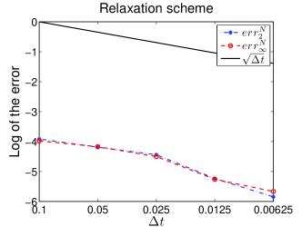
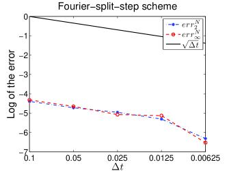
Figure 1: Plot of the log of the relative errors $\text{err}_{2}^{N}$ and $\text{err}_{\infty}^{N}$ respectively for the scheme (4.10) and (4.13)

5 Proof of Lemma 2.2 and Proposition 3.2

5.1 Proof of Lemma 2.2

The proof of this lemma is divided into two parts. In a first step, we prove inequality (2.21). The second step consists in proving estimate (2.23); the same arguments are used to deduce the bound (2.22) from (2.21).

Proof of estimate (2.21).

We begin this proof with a lemma stating that $\mathcal{V}^{l}_{\Delta t}$ is almost surely a bounded operator in $\mathds{L}^{2}$ with a random continuity constant.

Lemma 5.1.

The random matrix operator $\mathcal{V}^{l}_{\Delta t}$ is almost surely a bounded operator in $\mathds{L}^{2}$ and for any $l=0,\cdots,n,$

$$\left\|\mathcal{V}^{l}_{\Delta t}f\right\|_{\mathds{L}^{2}}\leqslant C_{0,l}\left(\omega\right)\left\|f\right\|_{\mathds{L}^{2}},$$

such that for all $p\geqslant 1$, there exists a constant $C(p)$ independent of $n$,

$$\mathds{E}\left(\max_{n\in\llbracket 1,N\rrbracket}C_{0,n}^{2p}\right)<C(p).$$

Proof.

By unitary property of the matrices $U_{\Delta t,l}$, for any $l=0,\cdots,n$, and applying Plancherel theorem and Hölder inequality,

$$\left\|\mathcal{V}^{l}_{\Delta t}f\right\|_{\mathds{L}^{2}}\leqslant\sup_{\xi\in\mathds{R}}M_{\Delta t,l}(\xi,\omega)\left\|f\right\|_{\mathds{L}^{2}},$$

where $M_{\Delta t,l}(\xi,\omega)=\left\|\left|m_{\Delta t,0}\left(\xi\right)\right|\right\|_{\infty}\left\|\left|m^{-1}_{\Delta t,l}\left(\xi\right)\right|\right\|_{\infty}$, where $m_{\Delta t,l}$ is the Fourier multiplier associated to the operator $T_{\Delta t,l}$. We claim that the random variable $M_{\Delta t,l}(\xi,\omega)$ is almost surely bounded by a constant $C_{0,l}(\omega)$, independent of $\xi$, that is integrable at any order. Indeed,

$$M_{\Delta t,l}(\xi,\omega)\leqslant\frac{1}{4\left|\det(l,\xi)\right|}\left(4+4\Delta t\left|\xi\right|^{2}+\Delta t^{2}\left|\xi\right|^{4}+2\sqrt{\gamma\Delta t}\left|\xi\right|\sum_{k=1}^{3}\left(\left|\chi_{k}^{0}\right|+\left|\chi_{k}^{l}\right|\right)\right)$$

$$+\frac{1}{4\left|\det(l,\xi)\right|}\left(\sqrt{\gamma\Delta t}\Delta t\left|\xi\right|^{3}\sum_{k=1}^{3}\left(\left|\chi_{k}^{0}\right|+\left|\chi_{k}^{l}\right|\right)+\gamma\Delta t\left|\xi\right|^{2}\sum_{k=1}^{3}\left|\chi_{k}^{0}\right|\sum_{k=1}^{3}\left|\chi_{k}^{l}\right|\right),$$ (5.1)

where $\det(l,\xi)$ is the determinant of $m_{\Delta t,l}$ and is given by

$$\det(l,\xi)=1+\frac{\gamma\Delta t}{4}\sum_{k=1}^{3}\left(\chi_{k}^{l}\right)^{2}\left|\xi\right|^{2}-\frac{\Delta t^{2}}{4}\left|\xi\right|^{4}-i\Delta t\left|\xi\right|^{2}.$$

Denoting $x=\Delta t^{1/2}\left|\xi\right|$ and $y=\sum_{k=1}^{3}\left(\chi_{k}^{l}\right)^{2}$, we define the mapping $f$ from $\mathds{R}^{2}_{+}$ into $\mathds{R}_{+}$

$$f(x,y)=\left(1+\frac{\gamma x^{2}}{4}y-\frac{x^{4}}{4}\right)^{2}+x^{4}.$$

It can be proved that

$$f(x,y)\geqslant\left\{\begin{array}[]{ll}\dfrac{1}{4}(1+x^{4})&\text{if }x^{2}\leqslant 4\max\left(\dfrac{\gamma y}{4},1\right)\\[4.26773pt] x^{4}&\text{if }4\max\left(\dfrac{\gamma y}{4},1\right)<x^{2}\leqslant 16\max\left(\dfrac{\gamma y}{4},1\right)\\[4.26773pt] \dfrac{1}{32}x^{8}+x^{4}&\text{if }x^{2}>16\max\left(\dfrac{\gamma y}{4},1\right).\end{array}\right.$$ (5.2)

Thus, there exists a positive constant $C$, such that for any $y\in\mathds{R}_{+}$ and any $\xi\in\mathds{R}$

$$M_{\Delta t,l}(\xi,\omega)<\ C \left(1+\max\left(\frac{\gamma y}{4},1\right)+\sqrt{\gamma}\sum_{k=1}^{3}\left(\left|\chi_{k}^{0}\right|+\left|\chi_{k}^{l}\right|\right)\left(1+\max\left(\frac{\gamma y}{4},1\right)^{1/2}\right)\right.$$

$$\left.+\gamma\sum_{k=1}^{3}\left|\chi_{k}^{0}\right|\sum_{k=1}^{3}\left|\chi_{k}^{l}\right|\right).$$

Therefore, $M_{\Delta t,l}(\xi,\omega)$ is uniformly bounded in $\xi$ by a polynomial function of $y$, $\left|\chi_{k}^{0}\right|$ and $\left|\chi_{k}^{l}\right|$. Applying the Cauchy-Schwarz inequality and the Burkholder-Davis-Gundy inequality, we obtain that $\mathds{E}\left(\max_{n\in\llbracket 1,N\rrbracket}M_{\Delta t,n}(\xi)^{2p}\right)$ is bounded by a constant independent of $n$. ∎

We now state a Lemma giving an estimate of the local error between the unbounded random operator $T_{\Delta t,n-1}U^{-1}_{\Delta t,n}T^{-1}_{\Delta t,n}$ and the identity mapping. This Lemma will be used to prove inequality (2.21).

Lemma 5.2.

For any $n\in\mathds{N}$, there exists a positive random constant $C_{n-1,n}(\omega)<+\infty$ a.s. belonging to $L^{2p}\left(\Omega\right),p\geqslant 1$, such that for any $f\in\mathds{H}^{1}$

$$\left\|\left[T_{\Delta t,n-1}U^{-1}_{\Delta t,n}T^{-1}_{\Delta t,n}-\text{I\footnotesize{d}}\right]f\right\|_{\mathds{L}^{2}}\leqslant C_{n-1,n}(\omega)\sqrt{\Delta t}\left\|f\right\|_{\mathds{H}^{1}}\qquad a.s.$$

Moreover, for all $p\geqslant 1$, there exists a constant $C(p)$ independent of $n$,

$$\mathds{E}\left(\max_{n\in\llbracket 1,N\rrbracket}C_{n-1,n}^{2p}\right)<C(p).$$

Proof.

From the proof of Lemma 5.1, we easily deduce that there exists a random variable $C_{n-1,n}(\omega)$, integrable at any order, such that

$$\sup_{\xi\in\mathds{R}}\frac{1}{\left(1+\left|\xi\right|^{2}\right)^{1/2}}\left\|\left|\widehat{T}_{\Delta t,n-1}\widehat{U}^{-1}_{\Delta t,n}\widehat{T}^{-1}_{\Delta t,n}-\text{I\footnotesize{d}}\right|\right\|_{\infty}\leqslant C_{n-1,n}(\omega)\sqrt{\Delta t},$$

where $C_{n-1,n}(\omega)$ is a polynomial function of $\sum_{k=1}^{3}\left(\chi_{k}^{n}\right)^{2}$, $\left|\chi_{k}^{n-1}\right|$ and $\left|\chi_{k}^{n}\right|$. The Cauchy-Schwarz and the Burkholder-Davis-Gundy inequalities imply that $\mathds{E}\left(\max_{n\in\llbracket 1,N\rrbracket}C_{n-1,n}^{2p}\right)$ is bounded by a constant independent of $n$. ∎

Now, we prove estimate (2.21). For any $l\geqslant 2$

$$\mathcal{V}^{l-1}_{\Delta t}-\mathcal{V}^{l-2}_{\Delta t}=\mathcal{V}^{l-2}_{\Delta t}\left[\left(\text{I\footnotesize{d}}+\frac{1}{2}H_{\Delta t,l-2}\right)\left(\text{I\footnotesize{d}}-\frac{1}{2}H_{\Delta t,l-1}\right)^{-1}-\text{I\footnotesize{d}}\right].$$

Therefore applying Lemma 5.1 and 5.2, and using the Cauchy-Schwarz inequality, we deduce that

$$\mathds{E} \left(\max_{n\in\llbracket 1,N\rrbracket}\left\|\sum_{l=1}^{n}\left(\mathcal{V}^{l-1}_{\Delta t}-\mathcal{V}^{l-2}_{\Delta t}\right)f^{l}\right\|_{\mathds{L}^{2}}^{2p}\right)$$

$$\leqslant N^{2p}\mathds{E}\left(\max_{n\in\llbracket 1,N\rrbracket}\left(C_{0,n-2}\right)^{2p}\left\|\left[T_{\Delta t,n-2}U^{-1}_{\Delta t,n-1}T^{-1}_{\Delta t,n-1}-\text{I\footnotesize{d}}\right]f^{n}\right\|_{\mathds{L}^{2}}^{2p}\right)$$

$$\leqslant T^{p}N^{p}\mathds{E}\left(\max_{n\in\llbracket 1,N\rrbracket}\left(C_{0,n-2}\right)^{4p}\left(C_{n-2,n-1}\right)^{4p}\right)^{1/2}\mathds{E}\left(\max_{n\in\llbracket 1,N\rrbracket}\left\|f^{n}\right\|_{\mathds{H}^{1}}^{4p}\right)^{1/2}.$$

Thus by Lemma 5.1, the following inequality holds

$$\mathds{E}\left(\max_{n\in\llbracket 1,N\rrbracket}\left\|\sum_{l=1}^{n}\left(\mathcal{V}^{l-1}_{\Delta t}-\mathcal{V}^{l-2}_{\Delta t}\right)f^{l}\right\|_{\mathds{L}^{2}}^{2p}\right)\leqslant C(\gamma,T,p)N^{p}\mathds{E}\left(\max_{n\in\llbracket 1,N\rrbracket}\left\|f^{n}\right\|_{\mathds{H}^{1}}^{4p}\right)^{1/2}.$$

Proof of estimate (2.23) for $q=1$.

Writing $\widetilde{X}(s)=\widetilde{X}^{l-1}+\widetilde{e}^{\,l-1}$, we rewrite $\epsilon_{1,1}^{l-1}$, given in (2.14), as follows

$$\epsilon_{1,1}^{l-1}=iC_{\gamma}\left(W_{0,0}^{l-1,l}\left(\partial^{4}_{x}\,\widetilde{e}^{\,l-1}\right)-\frac{1}{2}W_{0}^{l-1,l}\left(\partial^{4}_{x}\,\widetilde{e}^{\,l-1}\right)\Delta t\right).$$

We focus on the first term in the above expression, the other term being bounded in a similar way. Using the Minkowski inequality, the contraction property of $\mathcal{U}_{\Delta t}^{n,l}$ in $\mathds{L}^{2}\left(\mathds{R}\right)$ for every $l\in\llbracket 1,n\rrbracket$ and the conservation of the $\mathds{H}^{4}$ norm, we get

$$\mathds{E}\left(\max_{n\in\llbracket 1,N\rrbracket}\left\|\sum_{l=1}^{n}\mathcal{U}^{n,l}_{\Delta t}W_{0,0}^{l-1,l}(\partial_{x}^{4}\,\widetilde{e}^{\,l-1})\right\|_{\mathds{L}^{2}}^{2p}\right)$$ (5.3)

$$\leqslant \mathds{E}\left(\left(\sum_{l=1}^{N}\sup_{t_{l-1}\leqslant u\leqslant t_{l}}\left\|\partial_{x}^{4}\,\widetilde{e}^{\,l-1}(u)\right\|_{\mathds{L}^{2}}\frac{\Delta t^{2}}{2}\right)^{2p}\right)$$

$$\leqslant C\left(\left\|X_{0}\right\|_{\mathds{H}^{4}}^{2p}\right)T^{2p}\Delta t^{2p}\left(1+\gamma^{p}\right).$$

Let us notice that after integration by part, the term $\epsilon_{1,2}^{l-1}$ whose expression is given in (2.15), can be written as follows

$$\epsilon_{1,2}^{l-1} = -i\sqrt{\gamma}\sum_{k=1}^{3}\sigma_{k}\partial^{3}_{x}\widetilde{X}^{l-1}\left(\frac{1}{2}W_{k}^{l-1}(1)\Delta t-W_{0,k}^{l-1,l}(1)\right)$$

$$-i\sqrt{\gamma}\sum_{k=1}^{3}\left(W_{0,k}^{l-1,l}\left(\sigma_{k}\partial^{3}_{x}\,\widetilde{e}^{\,l-1}\right)-\frac{1}{2}W_{k}^{l-1,l}\left(\sigma_{k}\partial^{3}_{x}\,\widetilde{e}^{\,l-1}\right)\Delta t\right).$$

Since $\mathcal{V}^{l-2}_{\Delta t}\sigma_{k}\partial^{3}_{x}\widetilde{X}^{l-1}$ is $\mathcal{F}_{l-1}$ adapted, the next equality holds

$$\mathcal{V}^{l-2}_{\Delta t}\sigma_{k}\partial^{3}_{x}\widetilde{X}^{l-1}W_{0,k}^{l-1,l}\left(1\right)=W_{0,k}^{l-1,l}\left(\mathcal{V}^{l-2}_{\Delta t}\sigma_{k}\partial^{3}_{x}\widetilde{X}^{l-1}\right).$$

In expression (5.1), all the terms may be bounded using similar arguments. So, we only do the computation for the above term. By orthogonality of the increments of the three dimensional Brownian Motion,

$$\mathds{E}\left(W_{0,k}^{l-1,l}\left(\mathcal{V}^{l-2}_{\Delta t}\sigma_{k}\partial^{3}_{x}\widetilde{X}^{l-1}\right)W_{0,j}^{l^{\prime}-1,l^{\prime}}\left(\mathcal{V}^{l^{\prime}-2}_{\Delta t}\sigma_{j}\partial^{3}_{x}\widetilde{X}^{l^{\prime}-1}\right)\right)=0\qquad\text{if }l\neq l^{\prime}\ \text{or }k\neq j.$$

Hence, we obtain

$$\ll\sum_{l=1}^{n}\sum_{k=1}^{3}W_{0,k}^{l-1,l}\left(\mathcal{V}^{l-2}_{\Delta t}\sigma_{k}\partial^{3}_{x}\widetilde{X}^{l-1}\right)\gg=\sum_{l=1}^{n}\sum_{k=1}^{3}\ll W_{0,k}^{l-1,l}\left(\mathcal{V}^{l-2}_{\Delta t}\sigma_{k}\partial^{3}_{x}\widetilde{X}^{l-1}\right)\gg,$$

where $\ll.\gg$ denotes the quadratic variation process. Thanks to the conservation of the $\mathds{H}^{m}$ norms, the solution $X$ of Equation (2.1) has all its moments bounded in $\mathds{H}^{m}$ and the stochastic integral is a true martingale. Thus, applying the Burkholder-Davis-Gundy inequality, Lemma 5.1 and Cauchy-Schwarz inequality, yields

$$\mathds{E} \left(\max_{n\in\llbracket 1,N\rrbracket}\gamma^{p}\left\|\sum_{l=1}^{n}\sum_{k=1}^{3}W_{0,k}^{l-1,l}\left(\mathcal{V}^{l-2}_{\Delta t}\sigma_{k}\partial^{3}_{x}\widetilde{X}^{l-1}\right)\right\|_{\mathds{L}^{2}}^{2p}\right)$$

$$\leqslant CT^{p}\gamma^{p}\Delta t^{2p}\mathds{E}\left(\max_{n\in\llbracket 1,N\rrbracket}\left[C_{0,n-2}\right]^{2p}\left\|\partial^{3}_{x}\widetilde{X}^{n-1}\right\|_{\mathds{L}^{2}}^{2p}\right)$$

$$\leqslant CT^{p}\gamma^{p}\Delta t^{2p}\mathds{E}\left(\max_{n\in\llbracket 1,N\rrbracket}\left[C_{0,n-2}\right]^{4p}\right)^{1/2}\mathds{E}\left(\max_{n\in\llbracket 1,N\rrbracket}\left\|\partial^{3}_{x}\widetilde{X}^{n-1}\right\|_{\mathds{L}^{2}}^{4p}\right)^{1/2}.$$ (5.5)

Hence, a bound follows from the conservation of the $\mathds{H}^{m}$ norms and Lemma 5.1. Collecting the above estimates (5.3) and (5.1) leads to the bound (2.23) for $q=1$.

Proof of estimate (2.23) for $q=2$.

The first and second terms $\epsilon^{l-1}_{2,1}$ and $\epsilon^{l-1}_{2,2}$ in (LABEL:secondterm) will give the order of convergence of the scheme. The third one $\epsilon^{l-1}_{2,3}$ may be bounded similarly as in the previous step. To bound $\epsilon^{l-1}_{2,1}$, we use again the Burkholder-Davis-Gundy inequality, the independence of the increments of the Brownian Motion, Lemma 5.1, Cauchy-Schwarz inequality and Lemma 2.1

$$\mathds{E} \left(\max_{n\in\llbracket 1,N\rrbracket}\gamma^{p}\left\|\sum_{l=1}^{n}\sum_{k=1}^{3}W_{k}^{l-1,l}\left(\mathcal{V}^{l-2}_{\Delta t}\sigma_{k}\partial_{x}\widetilde{e}^{\,l-1}\right)\right\|_{\mathds{L}^{2}}^{2p}\right)$$

$$\leqslant C\gamma^{p}\mathds{E}\left(\left(\sum_{l=1}^{N}\sum_{k=1}^{3}W_{0}^{l-1,l}\left(\left\|\mathcal{V}^{l-2}_{\Delta t}\sigma_{k}\partial_{x}\widetilde{e}^{\,l-1}\right\|_{\mathds{L}^{2}}^{2}\right)\right)^{p}\right)$$

$$\leqslant C(p,\gamma)\left\|X_{0}\right\|_{\mathds{H}^{2}}^{2p}T^{p}\Delta t^{p}.$$ (5.6)

We conclude the proof obtaining an estimate for $\epsilon^{l-1}_{2,2}$. Using Equation (2.8) and Property 1.1, we obtain the equality

$$\epsilon_{2,2}^{l-1} = \frac{3\gamma}{2}\frac{\partial^{2}\widetilde{X}^{l-1}}{\partial x^{2}}\Delta t-\frac{\gamma}{2}\sum_{k=1}^{3}\frac{\partial^{2}\widetilde{X}^{l-1}}{\partial x^{2}}\left(W^{l-1}_{k}(1)\right)^{2}$$

$$+\frac{3\gamma}{2}W_{0}^{l-1,l}\left(\partial_{x}^{2}\widetilde{e}^{\,l-1}\right)-\frac{\gamma}{2}\sum_{j,k=1}^{3}W_{j}^{l-1,l}\left(\sigma_{j}\sigma_{k}\partial_{x}^{2}\widetilde{e}^{\,l-1}\right)W^{l-1}_{k}(1).$$

Moreover,

$$\ll\left(W_{k}^{l-1,l}(1)\right)^{2}-\Delta t\gg=4\Delta t\left(W_{k}^{l-1,l}(1)\right)^{2}-2\Delta t^{2}.$$

Thus, applying the Burkholder-Davis-Gundy inequality, using the independence of the increments of the Brownian Motion, applying Lemma 5.1, using the conservation of the $\mathds{H}^{m}$ norms and the Cauchy-Schwarz inequality

$$\mathds{E} \left(\max_{n\in\llbracket 1,N\rrbracket}\left\|\sum_{l=1}^{n}\mathcal{V}^{l-2}_{\Delta t}\left(\frac{3\gamma}{2}\frac{\partial^{2}\widetilde{X}^{l-1}}{\partial x^{2}}\Delta t-\frac{\gamma}{2}\sum_{k=1}^{3}\frac{\partial^{2}\widetilde{X}^{l-1}}{\partial x^{2}}\left(W^{l-1}_{k}(1)\right)^{2}\right)\right\|_{\mathds{L}^{2}}^{2p}\right)$$

$$\leqslant C\gamma^{2p}\mathds{E}\left(\left(\sum_{l=1}^{N}\sum_{k=1}^{3}\left\|\mathcal{V}^{l-2}_{\Delta t}\frac{\partial^{2}\widetilde{X}^{l-1}}{\partial x^{2}}\left(4\Delta t\left(W_{k}^{l-1}(1)\right)^{2}-2\Delta t^{2}\right)\right\|_{\mathds{L}^{2}}\right)^{p}\right)$$

$$\leqslant C\left\|X_{0}\right\|_{\mathds{H}^{2}}^{2p}\gamma^{2p}N^{p-1}\sum_{l=1}^{N}\sum_{k=1}^{3}\mathds{E}\left(\left(C_{0,l-2}\right)^{p}\left|4\Delta t\left(W_{k}^{l-1}(1)\right)^{2}-2\Delta t^{2}\right|^{p}\right)$$

$$\leqslant C\left\|X_{0}\right\|_{\mathds{H}^{2}}^{2p}\gamma^{2p}T^{p}\Delta t^{p}.$$ (5.7)

The last term $\epsilon^{n}_{2,3}$ in (LABEL:secondterm) may be bounded similarly as $\epsilon^{n}_{1,2}$. Estimate (2.23) for $q=2$ is obtained collecting bounds (5.6) and (5.1).

5.2 Proof of Proposition 3.2

Before proving Proposition 3.2, let us state two useful Lemmas. The first result gives uniform bounds for the solution $X_{R}$ of the cut-off equation (3.3).

Lemma 5.3.

Let $X_{0}\in\mathds{H}^{6}$ and $X_{R}$ be the solution of (3.3); then for all $T>0$ there exists a positive constant $C_{3}\left(R,T,\left\|X_{0}\right\|_{\mathds{H}^{6}}\right)$, such that, a.s for every $t$ in $[0,T]$,

$$\left\|X_{R}(t)\right\|_{\mathds{H}^{6}}\leqslant C_{3}\left(R,T,\left\|X_{0}\right\|_{\mathds{H}^{6}}\right).$$

Moreover, the function $T\mapsto C_{3}\left(R,T,\left\|X_{0}\right\|_{\mathds{H}^{6}}\right)$ is a continuous function from $\mathds{R}_{+}$ to $\mathds{R}_{+}$ and then is bounded on every compact set of $\mathds{R}_{+}$. We denote by $\widetilde{C}_{3}\left(R,T,\left\|X_{0}\right\|_{\mathds{H}^{6}}\right)$ the positive constant such that, a.s for every $t$ in $[0,T]$,

$$\left\|F\left(X_{R}(t)\right)\right\|_{\mathds{H}^{6}}\leqslant\widetilde{C}_{3}\left(R,T,\left\|X_{0}\right\|_{\mathds{H}^{6}}\right).$$

Proof of Lemma 5.3.

The proof is similar to the proof of Lemma $4.1$ in [6]. ∎

Let us now denote by $\widetilde{e}^{\,n}_{R}(s)$ the difference $\widetilde{e}^{\,n}_{R}(s)=X_{R}(s)-\widetilde{X}^{n}_{R}$ for all $s\in[t_{n},t_{n+1}]$ and state an intermediate result which gives a local estimate on $\widetilde{e}^{\,n}_{R}(s)$.

Lemma 5.4.

For any $p\geqslant 1$, if $X_{0}\in\mathds{H}^{2}$ then there exists a positive constant $C_{4}$, such that

$$\mathds{E}\left(\sup_{t_{l-1}\leqslant t\leqslant t_{l}}\left\|\widetilde{e}^{\,l-1}_{R}(t)\right\|_{\mathds{H}^{1}}^{2p}\right)\leqslant C_{4}(R,T,p,\gamma,\left\|X_{0}\right\|_{\mathds{H}^{2}})\Delta t^{p}\qquad\forall\ l=1,\cdots,N_{T}.$$

Moreover $C_{4}\equiv C_{p}(\gamma)C_{3}^{2p}(R,T,\left\|X_{0}\right\|_{\mathds{H}^{2}})+C(R)\Delta t^{p}$, where $C_{p}(\gamma)$ is given in Lemma 2.1, $C_{3}$ is given in Lemma 5.3 and $C(R)$ is a positive constant depending only on $R$.

Proof of Lemma 5.4.

This estimate is obtained using the Duhamel formulation (3.2), writing $X_{R}(t)$ in terms of $\widetilde{X}^{l-1}_{R}$, using Lemma 2.1 and 5.3 and because $G$ is globally Lipschitz. ∎

Let us now prove Proposition 3.2.

Proof of Proposition 3.2.

We split the difference as follows

$$U\left(t_{n},s\right)G\left(X_{R}(s)\right)-\mathcal{U}_{\Delta t}^{n,l}G\left(X^{l-1}_{R},X^{l}_{R}\right)=A_{1}^{l-1,l}+A_{2}^{l-1,l}+A_{3}^{l-1,l},$$

where

$$\left\{\begin{array}[]{ll}&A_{1}^{l-1,l}=\displaystyle{U(t_{n},s)\left(\Theta_{R}^{2}\left(X_{R}(s)\right)-\Theta_{X_{R}}^{l-1,l}\right)F\left(X_{R}(s)\right)}\\[14.22636pt] &A_{2}^{l-1,l}=\displaystyle{\left(U\left(t_{n},s\right)-\mathcal{U}_{\Delta t}^{n,l}\right)\Theta_{X_{R}}^{l-1,l}F\left(X_{R}(s)\right)}\\[14.22636pt] &A_{3}^{l-1,l}=\displaystyle{\mathcal{U}_{\Delta t}^{n,l}\Theta_{X_{R}}^{l-1,l}\left(F\left(X_{R}(s)\right)-F\left(X^{l-1}_{R},X^{l}_{R}\right)\right)}.\end{array}\right.$$ (5.11)

In order to obtain an estimate on the global error in $L^{2p}\left(\Omega\right)$, we decompose the term $X_{R}(s)-X^{l}_{R}$, appearing in $A_{1}^{l-1,l}$ and $A_{3}^{l-1,l}$, in two terms : $\widetilde{e}^{\,l}_{R}(s)$ and $e_{R}^{l}$. The first term gives the contribution to the final order and the second term may be handled by a fixed point procedure. Let us denote $\Theta_{X_{R}}^{l}=\Theta\left(\left\|X^{l}_{R}\right\|_{\mathds{H}^{1}}/R\right)$ for any $l=0,\cdots n$. Writing

$$\Theta_{R}^{2}\left(X_{R}(s)\right)-\Theta_{X_{R}}^{l-1,l}=\ \Theta_{R}\left(X_{R}(s)\right)\left(\Theta_{R}\left(X_{R}(s)\right)-\Theta_{X_{R}}^{l-1}\right)$$

$$-\Theta_{X_{R}}^{l-1}\left(\Theta_{R}\left(X_{R}(s)\right)-\Theta_{X_{R}}^{l}\right)$$

and using the isometric property of the random propagator $U$, the boundedness of $\Theta$ and $\Theta^{\prime}$ and the mean value theorem we obtain the following bound

$$\left\|\sum_{l=1}^{n}\int_{t_{l-1}}^{t_{l}}\Theta_{R}\left(X_{R}(s)\right)\left(\Theta_{R}\left(X_{R}(s)\right)-\Theta_{X_{R}}^{l-1}\right)U(t_{n},s)F\left(X_{R}(s)\right)ds\right\|_{\mathds{H}^{1}}^{2p}$$

$$\leqslant\left(\sum_{l=1}^{n}CR^{3}\int_{t_{l-1}}^{t_{l}}\frac{\left\|\Theta^{\prime}\right\|_{L^{\infty}}}{R}\left(\left\|\widetilde{e}^{\,l-1}_{R}(s)\right\|_{\mathds{H}^{1}}+\left\|e^{\,l-1}_{R}\right\|_{\mathds{H}^{1}}\right)ds\right)^{2p}.$$

By the same arguments, together with Lemma 5.3 and 5.4, we obtain

$$\mathds{E}\left(\max_{n\in\llbracket 1,N\rrbracket}\left\|\sum_{l=1}^{n}A_{1}^{l-1,l}\right\|_{\mathds{H}^{1}}^{2p}\right)\leqslant C_{5}(R,T,p)\left[C_{4}(R,T,p,\gamma,\left\|X_{0}\right\|_{\mathds{H}^{2}})\Delta t^{p}+\mathds{E}\left(\max_{n\in\llbracket 1,N\rrbracket}\left\|e^{n}_{R}\right\|_{\mathds{H}^{1}}^{2p}\right)\right].$$

where $C_{5}\equiv C^{2p}R^{4p}T^{2p}.$ Now, we split the term $A_{2}^{l-1,l}$ further

$$A_{2}^{l-1,l} = \int_{t_{l-1}}^{t_{l}}U\left(t_{n},s\right)\left(\text{I\footnotesize{d}}-U\left(s,t_{l-1}\right)\right)\Theta_{X_{R}}^{l-1,l}F\left(X_{R}(s)\right)ds$$

$$+\int_{t_{l-1}}^{t_{l}}\left(U\left(t_{n},t_{l-1}\right)-\mathcal{U}_{\Delta t}^{n,l}\right)\Theta_{X_{R}}^{l-1,l}F\left(X_{R}(s)\right)ds$$

$$= A_{2,1}^{l-1,l}+A_{2,2}^{l-1,l}.$$

The first term in the above equality can easily be estimated using again the isometric property of the random propagator $U\left(t_{n},s\right)$ and Hölder inequality, together with Lemma 5.3 and 2.1,

$$\mathds{E}\left(\max_{n\in\llbracket 1,N\rrbracket}\left\|\sum_{l=1}^{n}A_{2,1}^{l-1,l}\right\|_{\mathds{H}^{1}}^{2p}\right)\leqslant C_{6}(R,T,p,\gamma,\left\|X_{0}\right\|_{\mathds{H}^{2}})\Delta t^{p}.$$

On the contrary, the second term $A_{2,2}^{l-1,l}$ cannot be bounded directly because we do not have an explicit representation (in Fourier space) of the random propagator $U(t,s)$, $t,s\in\mathds{R}_{+},t\geqslant s$, solution of the linear equation (2.1). Writing

$$\mathcal{U}_{\Delta t}^{n,l}=U_{\Delta t,n}\cdots U_{\Delta t,l-1}\left(\text{I\footnotesize{d}}-\frac{1}{2}H_{\Delta t,l-1}\right)^{-1},$$

we split $A_{2,2}^{l-1,l}$ as follows

$$A_{2,2}^{l-1,l} = \int_{t_{l-1}}^{t_{l}}\left(U\left(t_{n},t_{l-1}\right)-\mathcal{U}_{\Delta t}^{n,l}\right)\Theta_{X_{R}}^{l-1,l}\left(F\left(X_{R}(s)\right)-F\left(\widetilde{X}^{l-1}_{R}\right)\right)ds$$

$$+\int_{t_{l-1}}^{t_{l}}\Theta_{X_{R}}^{l-1,l}\left(U\left(t_{n},t_{l-1}\right)-U_{\Delta t,n}\cdots U_{\Delta t,l-1}\right)F\left(\widetilde{X}^{l-1}_{R}\right)ds$$

$$+\int_{t_{l-1}}^{t_{l}}\Theta_{X_{R}}^{l-1,l}U_{\Delta t,n}\cdots U_{\Delta t,l-1}\left(\text{I\footnotesize{d}}-\left(\text{I\footnotesize{d}}-\frac{1}{2}H_{\Delta t,l-1}\right)^{-1}\right)F\left(\widetilde{X}^{l-1}_{R}\right)ds$$

$$= A_{2,2,1}^{l-1,l}+A_{2,2,2}^{l-1,l}+A_{2,2,3}^{l-1,l}.$$

The first term $A_{2,2,1}^{l-1,l}$ is easily bounded thanks to the local Lipschitz property of the nonlinear function $F$, the isometric property of both $U\left(t_{n},t_{l-1}\right)$ and $\mathcal{U}_{\Delta t}^{n,l}$, the boundedness of $\Theta$ and Lemma 5.3. This leads to

$$\mathds{E}\left(\max_{n\in\llbracket 1,N\rrbracket}\left\|\sum_{l=1}^{n}A_{2,2,1}^{l-1,l}\right\|_{\mathds{H}^{1}}^{2p}\right)\leqslant C_{7}(R,T,p,\gamma,\left\|X_{0}\right\|_{\mathds{H}^{2}})\Delta t^{p}.$$ (5.12)

Let us now consider the second term $A_{2,2,2}^{l-1,l}$ that can be bounded using the linear estimate (2.7) obtained in Proposition 2.2 together with Lemma 5.3. In this way,

$$\mathds{E}\left(\max_{n\in\llbracket 1,N\rrbracket}\left\|\sum_{l=1}^{n}A_{2,2,2}^{l-1,l}\right\|_{\mathds{H}^{1}}^{2p}\right)\leqslant C_{8}(R,T,p,\gamma,\left\|X_{0}\right\|_{\mathds{H}^{6}})\Delta t^{p}.$$ (5.13)

An estimate on the last term $A_{2,2,3}^{l-1,l}$ is obtained thanks to the next result, whose proof is identical to Lemma 5.2.

Lemma 5.5.

For any $n\in\mathds{N}$, there exists a positive random constant $C_{n}(\omega)<+\infty$ a.s. belonging to $L^{2p}\left(\Omega\right),p\geqslant 1$, whose moments are independent of $n$, such that for any $f\in\mathds{H}^{1}$

$$\left\|\left[\text{I\footnotesize{d}}-\left(\text{I\footnotesize{d}}-\frac{1}{2}H_{\Delta t,n}\right)^{-1}\right]f\right\|_{\mathds{L}^{2}}\leqslant C_{n}(\omega)\sqrt{\Delta t}\left\|f\right\|_{\mathds{H}^{1}}\qquad a.s.$$

Moreover for any $p\geqslant 1$, there exists a constant $C(p)$ independent of $n$ such that

$$\mathds{E}\left(\max_{n\in\llbracket 1,N\rrbracket}C_{n}^{2p}\right)<C(p).$$

From this Lemma, we easily obtain a bound on the last term $A_{2,2,3}$. Combining the above estimates (5.12), (5.13), we obtain an estimate on $A^{l-1,l}_{2,2}$

$$\mathds{E}\left(\max_{n\in\llbracket 1,N\rrbracket}\left\|\sum_{l=1}^{n}A^{l-1,l}_{2,2}\right\|_{\mathds{H}^{1}}^{2p}\right)\leqslant C_{9}(R,T,p,\gamma,\left\|X_{0}\right\|_{\mathds{H}^{6}})\Delta t^{p}.$$

Finally, we bound the last term $A_{3}^{l-1,l}$ splitting it as follows

$$A_{3}^{l-1,l} = \int_{t_{l-1}}^{t_{l}}\mathcal{U}_{\Delta t}^{n,l}\Theta_{X_{R}}^{l-1,l}\left(F\left(X_{R}(s)\right)-F\left(\widetilde{X}^{l-1}_{R},\widetilde{X}^{l-1}_{R}\right)\right)ds$$

$$+\int_{t_{l-1}}^{t_{l}}\mathcal{U}_{\Delta t}^{n,l}\Theta_{X_{R}}^{l-1,l}\left(F\left(\widetilde{X}^{l-1}_{R},\widetilde{X}^{l-1}_{R}\right)-F\left(\widetilde{X}^{l-1}_{R},\widetilde{X}^{l}_{R}\right)\right)ds$$

$$+\int_{t_{l-1}}^{t_{l}}\mathcal{U}_{\Delta t}^{n,l}\Theta_{X_{R}}^{l-1,l}\left(F\left(\widetilde{X}^{l-1}_{R},\widetilde{X}^{l}_{R}\right)-F\left(X^{l-1}_{R},X^{l}_{R}\right)\right)ds$$

$$= A_{3,1}^{l-1,l}+A_{3,2}^{l-1,l}+A_{3,3}^{l-1,l}.$$

Note that by Lemma 3.1, the last term $A_{3,3}^{l-1,l}$ is easily bounded as follows

$$\mathds{E}\left(\max_{n\in\llbracket 1,N\rrbracket}\left\|\sum_{l=1}^{n}A^{l-1,l}_{3,3}\right\|_{\mathds{H}^{1}}^{2p}\right)\leqslant C_{10}(R,T,p)\mathds{E}\left(\max_{n\in\llbracket 1,N\rrbracket}\left\|e^{n}_{R}\right\|_{\mathds{H}^{1}}^{2p}\right),$$

where $C_{10}\equiv C^{2p}R^{4p}T^{2p}$. The first term $A_{3,1}^{l-1,l}$ is bounded using $F\left(\widetilde{X}^{l-1}_{R},\widetilde{X}^{l-1}_{R}\right)=F\left(\widetilde{X}^{l-1}_{R}\right)$, Lemma 5.3, Hölder inequality and Lemma 5.4. An estimate on the second term $A_{3,2}^{l-1,l}$ may be obtained using Lemma 5.3 and Lemma 5.4. ∎

6 Conclusion

The evolution of the slowly varying envelopes driven by random polarization mode dispersion is described by the stochastic Manakov equation. We introduce three different schemes for this equation using a semi-implicit discretization of the Stratonovich integrals. We prove that the CN scheme is of order $1/2$ and is conservative for the discrete $\mathds{L}^{2}$ norm, contrarily to a scheme based on the Itô formulation. This method may be applied to other stochastic equations written in Stratonovich form and especially for equations with conservation laws.

References

- [1] C. Besse. A relaxation scheme for the nonlinear Schrödinger equation. SIAM J. Numer. Anal., 42(3):934–952, 2004.
- [2] A. M. Davie and J. G. Gaines. Convergence of numerical schemes for the solution of parabolic stochastic partial differential equations. Math. Comp., 70(233):121–134, 2001.
- [3] A. de Bouard and A. Debussche. A stochastic nonlinear Schrödinger equation with multiplicative noise. Comm. Math. Phys., 205(1):161–181, 1999.
- [4] A. De Bouard and A. Debussche. A semi-discrete scheme for the stochastic nonlinear Schrödinger equation. Numer. Math., 96(4):733–770, 2004.
- [5] A. de Bouard and A. Debussche. Weak and strong order of convergence of a semidiscrete scheme for the stochastic nonlinear Schrödinger equation. Appl. Math. Optim., 54(3):369–399, 2006.
- [6] A. de Bouard and M. Gazeau. A diffusion approximation theorem for a nonlinear PDE with application to random birefringent optical fibers. Ann. Appl. Probab., 22(6):2460–2504, 2012.
- [7] A. Debussche. Weak approximation of stochastic partial differential equations: the nonlinear case. Math. Comp., 80(273):89–117, 2011.
- [8] A. Debussche and J. Printems. Numerical simulation of the stochastic Korteweg-de Vries equation. Phys. D, 134(2):200–226, 1999.
- [9] A. Debussche and J. Printems. Convergence of a semi-discrete scheme for the stochastic Korteweg-de Vries equation. Discrete Contin. Dyn. Syst. Ser. B, 6(4):761–781 (electronic), 2006.
- [10] A. Debussche and J. Printems. Weak order for the discretization of the stochastic heat equation. Math. Comp., 78(266):845–863, 2009.
- [11] M. Delfour, M. Fortin, and G. Payre. Finite-difference solutions of a nonlinear Schrödinger equation. J. Comput. Phys., 44(2):277–288, 1981.
- [12] O. Faure. Simulation du Mouvement Brownien et des Diffusions. Thèse de Doctorat, Ecole des Ponts et Chaussées, 1992.
- [13] M. Gazeau. Analyse de modèles mathématiques pour la propagation de la lumière dans les fibres optiques en présence de biréfringence aléatoire. Thèse de Doctorat, Ecole Polytechnique, 2012.
- [14] M. Gazeau. Numerical simulation of nonlinear pulse propagation in optical fibers with randomly varying birefringence. preprint, 2013.
- [15] I. Gyöngy. Lattice approximations for stochastic quasi-linear parabolic partial differential equations driven by space-time white noise. I. Potential Anal., 9(1):1–25, 1998.
- [16] I. Gyöngy and A. Millet. On discretization schemes for stochastic evolution equations. Potential Anal., 23(2):99–134, 2005.
- [17] I. Gyöngy and D. Nualart. Implicit scheme for quasi-linear parabolic partial differential equations perturbed by space-time white noise. Stochastic Process. Appl., 58(1):57–72, 1995.
- [18] A. Hasegawa. Effect of polarization mode dispersion in optical soliton transmission in fibers. Physica D: Nonlinear Phenomena, 188(3-4):241–246, 2004.
- [19] E. Hausenblas. Approximation for semilinear stochastic evolution equations. Potential Anal., 18(2):141–186, 2003.
- [20] E. Hausenblas. Weak approximation of the stochastic wave equation. J. Comput. Appl. Math., 235(1):33–58, 2010.
- [21] P. E. Kloeden and E. Platen. Numerical solution of stochastic differential equations, volume 23 of Applications of Mathematics (New York). Springer-Verlag, Berlin, 1992.
- [22] R. Marty. On a splitting scheme for the nonlinear Schrödinger equation in a random medium. Commun. Math. Sci., 4(4):679–705, 2006.
- [23] A. Millet and P-L. Morien. On implicit and explicit discretization schemes for parabolic SPDEs in any dimension. Stochastic Process. Appl., 115(7):1073–1106, 2005.
- [24] G. N. Milstein. A method with second order accuracy for the integration of stochastic differential equations. Teor. Verojatnost. i Primenen., 23(2):414–419, 1978.
- [25] G. N. Milstein. Weak approximation of solutions of systems of stochastic differential equations. Teor. Veroyatnost. i Primenen., 30(4):706–721, 1985.
- [26] G. N. Milstein and M. V. Tretyakov. Stochastic numerics for mathematical physics. Scientific Computation. Springer-Verlag, Berlin, 2004.
- [27] G.N. Milstein, Y.P. Repin, and M.V Tretyakov. Mean-square symplectic methods for hamiltonian systems with multiplicative noise.
- [28] J. Printems. On the discretization in time of parabolic stochastic partial differential equations. M2AN Math. Model. Numer. Anal., 35(6):1055–1078, 2001.
- [29] T. R. Taha and M. J. Ablowitz. Analytical and numerical aspects of certain nonlinear evolution equations. II. Numerical, nonlinear Schrödinger equation. J. Comput. Phys., 55(2):203–230, 1984.
- [30] D. Talay. Résolution trajectorielle et analyse numérique des équations différentielles stochastiques. Stochastics, 9(4):275–306, 1983.
- [31] D. Talay. Discrétisation d’une équation différentielle stochastique et calcul approché d’espérances de fonctionnelles de la solution. RAIRO Modél. Math. Anal. Numér., 20(1):141–179, 1986.
- [32] P. K. A. Wai and C. R. Menyuk. Polarization mode dispersion, decorrelation, and diffusion in optical fibers with randomly varying birefringence. Journal of Lightwave Technology, 14(2):148–157, 1996.
- [33] J. A. C. Weideman and B. M. Herbst. Split-step methods for the solution of the nonlinear Schrödinger equation. SIAM J. Numer. Anal., 23(3):485–507, 1986.