CERN-PH-TH/2013-174

Abstract

Experimental data on the neutrino mixing and masses strongly suggest an underlying approximate symmetry of the relevant Yukawa superpotential terms. Intensive phenomenological explorations during the last decade indicate that permutation symmetries such as $S_{4}$, $A_{4}$ and their subgroups, under certain assumptions and vacuum alignments, predict neutrino mass textures compatible with such data. Motivated by these findings, in the present work we analyse the neutrino properties in F-theory GUT models derived in the framework of the maximal underlying $E_{8}$ symmetry in the elliptic fibration. More specifically, we consider local F-$SU(5)$ GUT models and study in detail spectral cover geometries with monodromies associated to the finite symmetries $S_{4},A_{4}$ and their transitive subgroups, including the dihedral group $D_{4}$ and ${Z}_{2}\times{Z}_{2}$. We discuss various issues that emerge in the implementation of $S_{4},A_{4}$ neutrino models in the F-theory context and suggest how these can be resolved. Realistic models are presented for the case of monodromies based on their transitive subgroups. We exemplify this procedure with a detailed analysis performed for the case of ${Z}_{2}\times{Z}_{2}$ model.

^♭ On leave from CPHT (UMR CNRS 7644) Ecole Polytechnique, F-91128 Palaiseau, France.

1 Introduction

F-theory Grand Unified Models (F-GUTs)[1, 2, 3, 4, 5] provide novel ways to compute Yukawa interactions which are capable of describing convincingly the observed fermion mass hierarchy. F-GUTs are associated to seven branes wrapping a complex surface $S$ in an elliptically fibered eight dimensional internal space . The precise gauge group is determined by the specific structure of the singular fibers over the compact surface $S$. Since $E_{8}$ is the highest symmetry of the elliptic fibration, the gauge symmetry of the effective model can in principle be any of the $E_{8}$ subgroups. Choosing $SU(5)_{GUT}$, one can in principle avoid exotic matter in the spectrum [3]. The gauge symmetry can be broken by turning on appropriate fluxes [2] which at the same time generate chirality for matter fields.

In these constructions matter fields are represented by wavefunctions on the intersections of seven branes with $S$. These intersections are two dimensional compact Riemann surfaces known as matter curves, along which, gauge symmetry is enhanced. When three such matter curves intersect at a point in the internal manifold, the symmetry is further augmented while a trilineal Yukawa coupling is formed. In viable F-theory models the top Yukawa coupling usually arises from a trilinear superpotential term. Its strength is then equal to the properly normalised integral of the product of the three overlapping wavefunctions corresponding to the states residing on the relevant matter curves. Two mechanisms have been suggested to obtain fermion mass hierarchy. If all families reside on the same matter curve, one way is to introduce non-commutative fluxes and take into account non-perturbative effects [10, 11, 12]. If however, fermion generations are distributed on different matter curves, hierarchy might emerge from a generalisation of the Froggat-Nilsen mechanism. It is likely of course that both mechanisms operate in particular constructions.

In F-theory models the implementation of the generalised Froggat-Nilsen mechanism is realised through the various discrete or abelian symmetries which appear in a natural way in any F-GUT construction[13, 14, 15, 16, 18, 17, 19, 20]. In the present work we focus on $SU(5)_{GUT}$ gauge group, so that such symmetries arise from the decomposition of $SU(5)_{\perp}$ i.e, the commutant with respect to initial $E_{8}$. GUT representations appear as bifundamentals under the $E_{8}\to SU(5)_{GUT}\times SU(5)_{\perp}$ breaking, and consequently the matter multiplets are characterised by the $SU(5)_{\perp}$’s residual symmetry. This final symmetry escorting the $SU(5)_{GUT}$ is the one left intact by certain monodromy actions which usually appear in F-theory compactifications. Such symmetries are extremely useful when -under certain circumstances- are used to implement the rôle of family symmetries. If properly chosen, they can provide the model with a hierarchical fermion mass spectrum and at the same time eliminate dangerous superpotential terms. Given the details of the internal manifold and the F-theory compactification, the specific nature of the residual symmetry might be any continuous or finite subgroup of $SU(5)_{\perp}$. As such, these can be the transitive groups of $S_{4}$, i.e. $A_{4},D_{4},Z_{4}$ etc, or abelian symmetries.

Within the above context, the last few years a considerable amount of work has been devoted to the study of the fermion mass hierarchy problem. Intensive studies focused on F-derived GUT models employing monodromies leading to discrete symmetries such as $Z_{2}$ and $Z_{3}$. These symmetries result to identifications of several matter curves a fact that could be adequate to allow for the existence of a tree-level Yukawa coupling -to be associated with the top quark- and predict a promising hierarchical charged fermion mass spectrum. However, we know that accumulating neutrino data reveal a rather different picture of the neutrino sector; this is characterised by large mixing angles  and apparent mild neutrino hierarchy as opposed to the large hierarchies and relatively small mixing of the quark sector. More than a decade ago, it has been observed that experimental neutrino data could be satisfactorily described in terms of charged and neutral lepton mass matrices which exhibit a particularly elegant structure. In this simple scheme, the mixing matrix takes the form

$$V_{TB} = V^{\dagger}_{l}V_{\nu}=\left(\begin{array}[]{lll}-\sqrt{\frac{2}{3}}&\frac{1}{\sqrt{3}}&0\\ \frac{1}{\sqrt{6}}&\frac{1}{\sqrt{3}}&-\frac{1}{\sqrt{2}}\\ \frac{1}{\sqrt{6}}&\frac{1}{\sqrt{3}}&\frac{1}{\sqrt{2}}\end{array}\right)$$ (1.4)

This structure is in accordance with $\sin^{2}\theta_{12}=1/3$, (for an approximate value $\theta_{12}\sim\pi/5$), and $\sin^{2}\theta_{23}=1/2$, (i.e. for $\theta_{23}=\pi/4$), while the third angle is exactly zero $\theta_{13}=0$. The above is called Tri-Bi (TB) maximal mixing [21]. In a basis where the charged lepton mass matrix is diagonal the most general neutrino mass texture diagonalised by the TB-mixing matrix is

$$m_{\nu}=\left(\begin{array}[]{lll}u&v&v\\ v&u+w&v-w\\ v&v-w&u+w\end{array}\right)$$ (1.5)

These observations suggested that there might be an invariance of the relevant Yukawa terms under some underlying symmetry involving finite groups such us $S_{4},A_{4}$ etc. The ensuing decade, accumulating experimental data have shown deviations from TB-mixing and that $\theta_{13}$ is not exactly zero. Nevertheless, such small departures from the exact symmetry can be related to various sources of symmetry breaking contributions such as radiative corrections etc.

Discrete symmetries have been found to play significant rôle in model building. They naturally emerge in string derived effective models and have been studied in various applications [22]. However, non-abelian discrete symmetries have only been recently investigated in a string context [23]. As we have mentioned above, they also arise naturally in the context of F-theory however, up to know little has been done to investigate their implications in model building[24].

Motivated by the apparent success of discrete groups in neutrino mixing, in this work we attempt to build models which incorporate monodromic actions entailing such finite symmetries. In particular we will rely on the $S_{4}$ and its transitive subgroups. In doing so, we will employ the techniques developed in the context of the spectral cover [5]. In particular, adopting the geometrical interpretation which associates the GUT symmetry to a divisor $S$ of the elliptically fibered internal manifold, we can use spectral covers to describe physics in its vicinity and extract useful properties of the model. In the elliptic fibration this can be described by the Tate model [25] and in the $SU(5)$ case, the spectral cover ${\cal C}_{5}$ is associated to a five degree polynomial whose coefficients encode useful information for the effective model. A natural way to attain symmetries such as $S_{4},A_{4},D_{4},{Z}_{2}\times{Z}_{2}$ etc, dictated by the neutrino sector, is to split the spectral cover to ${\cal C}_{5}\to{\cal C}_{4}\times{\cal C}_{1}$. We will see however, that the combined GUT-symmetry and internal geometry restrictions leave little room for a successful implementation of the larger finite groups such as $S_{4}$ and $A_{4}$. Notwithstanding these problems, such symmetries deserve a thorough study since one might evade many difficulties when the F-GUT symmetry is replaced by that of the F-theory Standard Model [26]. We leave such an analysis for future work whilst in the second part of the present paper we deal with a more realistic model which is based on the ${Z}_{2}\times{Z}_{2}$ family symmetry.

The paper is organised as follows. In section 2 we present the origin of the various discrete symmetries in F-theory while in section 3 we analyse in detail those emerging in $SU(5)_{GUT}$ models in the context of the spectral cover. In section 4 we analyse their implications on the neutrino sector in several effective models. In section 5 we present our conclusions. Finally in the Appendix we give details of the calculations.

2 The Origin of Family Symmetries in F-theory

As we have argued in the introduction, an attractive feature of F-theory models is the appearance of discrete symmetries which, among other consequences, govern the structure of the Yukawa sector of the effective low energy theory. We are particulary interested in non-abelian discrete symmetries which are quite appealing when dealing with the neutrino sector. The implementation of such a scenario in the effective model requires the study of the spectral cover construction and the description of the relevant monodromies. The most important issue however is the determination of the conditions on the manifold and fluxes related to the part of the spectral cover associated to the non-Abelian discrete gauge group. As we have already pointed out, the study of the local geometry is conveniently described by introducing the spectral surface ${\cal C}_{5}$. Guided by the neutrino phenomenology we will split this to ${\cal C}_{5}\to{\cal C}_{4}\times{\cal C}_{1}$. The above splitting associates the ${\cal C}_{4}$ part with a fourth degree polynomial and the ${\cal C}_{1}$ with the linear piece which corresponds to a $U(1)$. According to the well known procedure form type IIB-theories, if we turn on a flux along $U(1)$ we can induce chirality on the spectrum -transformed under $SU(5)_{GUT}$ and the remaining symmetry of the spectral cover- which is an essential step to build a viable model. It may also eliminate the colour triplet parts of the Higgs fiveplets which, had they remained in the spectrum, they would lead to proton decay at unacceptable rates. On the other hand the ${\cal C}_{4}$ part corresponding to the quartic polynomial induces a monodromy group which is a transitive subgroup of the non-abelian discrete symmetry $S_{4}$. To decide which the transitive subgroup is, this requires further knowledge of the structure of non-abelian fluxes as well as investigation of the topological properties of the coefficients of the associated quartic polynomial. In this paper we do not deal with the first issue which is a rather involved task. Nevertheless, from the point of view of the low energy field theory model and its phenomenological implications that we are examining in this work, it suffices to analyse the properties of the polynomial coefficients which constitute non-trivial sections and give all the necessary information to determine the matter spectrum. A second issue concerns the action of geometric symmetries on the matter wavefunctions. This is important because, even in the absence of the colour triplets in the presence of flux effects, there are still problematic Yukawa couplings that can be avoided only when matter parity is defined. We will explain how $Z_{2}$ symmetries of geometric origin can have such an effect. In doing so, we will follow [27] and argue that the manifold and flux data may turn to invariance properties of the spectral surface and see how this can translate into an action on the matter wavefunctions.

2.1 Monodromies and discrete symmetries

In the case of the elliptic fibration, the highest symmetry obtained is ${E}_{8}$, with all matter fields embedded in its adjoint representation. The most familiar models of F-theory origin are based either on the $SU(5)_{GUT}$ or $SO(10)_{GUT}$ groups. The first class in particular arises under the following breaking pattern

$$E_{8}\to SU(5)_{GUT}\times SU(5)_{\perp}$$

All $SU(5)_{GUT}$ matter representations have also transformation properties under the second group factor, denoted here as $SU(5)_{\perp}$, comprising the properties of the normal bundle. The decomposition of the adjoint representation of $E_{8}$ under $SU(5)_{GUT}\times SU(5)_{\perp}$ is

$$248=(24,1)+(1,24)+(10,5)+(\bar{5},10)+(\overline{10},\bar{5})+(5,\overline{10})$$

If we appeal to the geometric origin of these symmetries, we associate the fiber singularity to $SU(5)_{GUT}$ and interpret the $SU(5)_{\perp}$ as the group describing the bundle in the vicinity.

The representations containing the low energy fields reside on matter curves dubbed here $\Sigma_{10},\Sigma_{5}$ and characterised by the $SU(5)_{\perp}$ weights $t_{i}$. In general on the two distinct kinds of matter curves we may have

$$\begin{split}\Sigma_{10}&:n_{10}\times 10_{t_{i}}+\bar{n}_{\bar{10}}\times\overline{10}_{-t_{i}}\\ \Sigma_{5}&:n_{5}\times\bar{5}_{t_{i}+t_{j}}+\bar{n}_{\bar{5}}\times 5_{-t_{i}-t_{j}}\end{split}$$ (2.1)

where the integers $n_{i}$ count the number of corresponding representations which live on a particular matter curve. The required chirality of the fermion spectrum is generated when $n_{i}\neq\bar{n}_{i}$ and this happens when fluxes are turned on along appropriate directions inside $SU(5)_{\perp}$.

One would expect that $SU(5)_{\perp}$ reduces to four $U(1)$’s which would play the rôle of flavour symmetries in the formation of the Yukawa couplings. A more careful analysis shows that there is a variety of possibilities. In general one expects the existence of a non-trivial subgroup of the Weyl group $S_{5}$ of $SU(5)_{\perp}$.

A short description of the situations goes as follows: The roots of $SU(5)_{\perp}$ satisfy the spectral cover equation

$${\cal C}_{5}:\;b_{0}s^{5}+b_{2}s^{3}+b_{3}s^{2}+b_{4}s+b_{5}=0$$ (2.2)

The coefficient $b_{1}$ does not appear in the equation (2.2), because it represents the sum of the $SU(5)$ roots which is identically zero. We denote $t_{i}$ the roots of (2.2) and write

$${\cal C}_{5}:\;b_{0}\prod_{i=1}^{5}(s-t_{i})=0$$ (2.3)

Clearly the $b_{k}$ coefficients and $t_{i}$’s are related with the well known relations $b_{5}/b_{0}=t_{1}t_{2}t_{3}t_{4}t_{5},\cdots$ etc, when coefficients of the same power of $s$ are compared. Such relations will be exploited in the subsequence.

This equation describes the geometric nature of a local patch around the $SU(5)_{GUT}$ singularity. Then, the coefficients $b_{k}$ (assumed to belong in some field ${\cal F}$) carry the information of the geometry. However, to obtain the roots $t_{i}$ requires inversion of the equations $b_{k}(t_{i})$ and some solutions may not belong to the field ${\cal F}$ but to some ${\cal K}\supset{\cal F}$ ( the so called splitting field ${\cal K}$). This means that the corresponding symmetry may not be $U(1)$. Depending on the number of roots which lie outside ${\cal F}$, and the specific properties of the coefficients, the group maybe any subgroup of $S_{5}$, namely

$$S_{4},A_{4},Z_{n}\times Z_{m},n+m<5,\;\dots$$

Such symmetries are very important since they determine several properties of the matter curves and the spectrum of the model hosted on them.

2.2 Spectral cover discrete symmetries

A convenient way to prevent unwanted and dangerous terms in the Yukawa Lagrangian is the implementation of a discrete ($Z_{N}$) symmetry. Indeed, in most effective low energy supersymmetric models matter parity is usually associated to a $Z_{2}$ symmetry, so that dangerous proton decay Yukawa interactions are avoided. It has been shown [27] that such a symmetry in F-theory can have a geometric origin associated to the compactified space and the fluxes. Once such a transformation is identified it must be checked whether its action induces the appropriate matter parity on the wavefunctions of the matter fields residing on the relevant matter curves. Thus, for example one can assume a $Z_{2}$ background configuration and try to relate this symmetry with the local geometry. To start from a global geometry however, it is not an easy task but one can assume its existence in certain compactifications and work out the details locally near the GUT divisor. Under these assumptions a realisation is presented for a GUT divisor $S_{GUT}=\mathbb{P}^{2}$ and a $Z_{2}$ transformation map in reference [27]. Locally, the manifold and the flux data can be captured by the Higgs bundle on $S_{GUT}$ which in turn can be described using the notion of the spectral surface and the line bundles. In this context, it can be shown that a $Z_{2}$ symmetry in particular induces an $SU(3)$ rotation of the three-complex coordinates of the total space which act on spinors the same way. A simple bottom-up approach how to incarnate such discrete symmetries in local models was applied in[19] and could be described as follows. In F-theory, we may appeal to the geometric origin of the GUT symmetries and consider the latter as a divisor $S_{GUT}$ which locally can be covered by open patches $U_{a}\in S_{GUT}$  [27]. For simplicity, here we focus on a single trivialisation patch and take $s$ to be the coordinate along the fiber and demand that under the required geometric transformation the spectral cover equation should remain invariant up to an overall phase. To this end consider the transformation $\sigma$ where $s,b_{k}$ are mapped according to 

$$s(\sigma(p))\;=\;s(p)\,e^{i\phi},\;b_{k}(\sigma(p))\;=\;b_{k}(p)\,e^{i\xi}e^{-i(6-k)\phi}$$ (2.4)

Then each term in the spectral cover equation transforms the same way

$$b_{k}s^{5-k}\rightarrow e^{i\xi}b_{k}s^{5-k}$$ (2.5)

We can exploit this invariance to communicate a $Z_{N}$ symmetry to $S_{GUT}$. We take the phase $\phi$ to be

$$\phi=\frac{2\pi}{N}$$

where $N$ is an integer. Thus, choosing $N=2$ for example, we have $\phi=\pi$ and a $Z_{2}$ symmetry is realised with $s,b_{k}$ transforming according to

$$s\rightarrow-s,\;b_{k}\rightarrow(-1)^{k}e^{i\xi}\,b_{k}$$ (2.6)

while in the limit $N\to\infty$, we get $s\to s$ and $b_{k}\to e^{i\xi}b_{k},\forall k$. Such symmetries can be communicated [19] to the matter curves as well as to the representations accommodated on them, imposing restrictions on the possible interaction and Yukawa terms of the superpotential.

3 Non abelian discrete symmetries and fermion mass textures

The issue of the fermion mass hierarchical structure has been tackled in several recent works in the context of F-theory. The large hierarchy among the charged fermions (quarks and leptons) and the CKM mixing can be readily accommodated either by non commutative flux effects or by employing the Frogatt-Nielsen mechanism interpreting the surplus $U(1)$’s as family symmetries. Solutions for the large neutrino mixing have also been considered. In the $SU(5)$ case, right-handed neutrinos are identified as Kaluza-Klein modes [31, 32]. Yukawa couplings including such states generate a milder hierarchy and allow for a large mixing as required by the neutrino data. The fermion mass hierarchy issues have been considered mainly in cases of the $Z_{2}$ monodromies. In the present work, we pay particular attention to the neutrino sector. Because much phenomenological work has been devoted to interpret the large lepton mixing with the implementation of discrete non-abelian groups, we intend to explore such cases in the context of F-theory where these symmetries arise naturally. Successful finite groups reconciling the neutrino data include the permutation symmetries such as $S_{4}$ as well as some of its subgroups. Motivated by these approximate symmetries of the neutrino sector, in the next section we will consider the case of the ${\cal C}_{4}\times{\cal C}_{1}$ splitting of the spectral cover and attempt to derive the peculiar neutrino properties, i.e. the large mixing and the tiny neutrino mass scale.

3.1 ${\cal C}_{4}\times{\cal C}_{1}$ spectral cover in $SU(5)$

We will assume $SU(5)$ unified models with $SU(5)_{\perp}$ spectral covers. Finite symmetries such as $S_{4},A_{4}$ and their subgroups can be obtained directly by splitting the spectral cover according to ${\cal C}_{5}\to{\cal C}_{4}\times{\cal C}_{1}$, which implies the splitting of the polynomial as

$$\sum b_{k}s^{5-k}=(a_{1}+a_{2}s+a_{3}s^{2}+a_{4}s^{3}+a_{5}s^{4})(a_{6}+a_{7}s)$$ (3.1)

defined in terms of new coefficients $a_{i}$. The splitting (3.1) induces the breaking of $SU(5)_{\perp}$ to a Galois group (which is $S_{4}$ or some other subgroup) and a $U(1)$. More precisely, depending on the specific properties of $a_{1...5}$ coefficients the discrete group could be one of $S_{4},A_{4},D_{4},V_{4}={Z}_{2}\times{Z}_{2},Z_{2}$. We can deduce the topological properties of these coefficients by exploiting the relations $b_{k}(a_{i})$. These can be found by comparing coefficients of the same powers in (3.1). One finds the following relations

$$b_{0}=a_{5}a_{7},\;b_{5}=a_{1}a_{6},\;{\rm and}\;b_{k}=a_{6-k}a_{6}+a_{5-k}a_{7},\;{\rm for}\;k=1,2,3,4\,$$ (3.2)

We can readily find that the homologies satisfy relations of the form

$$[b_{k}]=[a_{l}]+[a_{12-l-k}]$$

for all combinations of indices appearing in (3.2). The $b_{k}$ topological properties are well defined and can be expressed in terms of the first Chern classes $c_{1}$ and $-t$ of the tangent and the normal bundle respectively. Thus, given that[4]

$$[b_{k}]=\eta-k\,c_{1},\;\eta=6c_{1}-t$$ (3.3)

all $[a_{i}]$ can be expressed in terms of one arbitrary parameter taken here to be $[a_{6}]=\chi$. These are presented in Table 1.

$a_{k}(k=1,\dots,5)$	$a_{6}$	$a_{7}$	$a_{0}$
$\eta-(6-k)c_{1}-\chi$	$\chi$	$c_{1}+\chi$	$\eta-2c_{1}-2\chi$

Table 1: Homology classes for coefficients $a_{i}$ for the ${\cal C}_{4}\times{\cal C}_{1}$ ($SU(5)$) case

To proceed further with the restrictions we impose the tracelessness condition $b_{1}=\sum_{i=1}^{5}t_{i}=0$ of $SU(5)_{\perp}$. The corresponding equation in (3.2) reads

$$a_{5}a_{6}+a_{4}a_{7}=0$$

and is solved by introducing a suitable coefficient $a_{0}$

$$a_{4}=\pm\,a_{0}a_{6},\;\;\;\;a_{5}=\mp\,a_{0}a_{7}$$ (3.4)

We discuss now the implications of these topological properties on the matter curves. The $SU(5)_{GUT}$ fiveplets transform as the $10\in SU(5)_{\perp}$ thus, we have a bifundamental $(5,\,10_{\perp})$. Denoting with $t_{i}$ the $SU(5)_{\perp}$ weights, the $5/\bar{5}^{\prime}s\in SU(5)_{GUT}$ are discriminated by the $\frac{1}{2}5(5-1)=10$ sheets of the spectral cover, with the assignments

$$t_{i}+t_{j},\;\;i<j=1,\dots,5$$

These are ‘roots’ of the relevant equation[5]

$${\cal P}_{5}(s)\propto\prod_{i<j}(s-t_{i}-t_{j})=s^{10}+\cdots+c_{1}\,s+c_{0}$$

The $c_{0}=\prod_{i,j}(t_{i}+t_{j})$ is a symmetric quantity thus, it can be expressed in terms of the $b_{k}$ coefficients. Consequently, the defining equation $P_{5}={\cal P}_{5}(0)$ for the GUT fiveplets is computed to be [5]

$$P_{5} = b_{4}b_{3}^{2}-b_{2}b_{5}b_{3}+b_{0}b_{5}^{2}$$ (3.5)

Hence, in principle there could be ten distinct curves (Riemann surfaces) accommodating the fiveplets, but the actual number equals the number of factors $P_{5}$ splits to. Plugging in the $a_{k}$ conditions enforced by the equation $b_{1}=0$ we see that this splits to two factors

$$P_{5}=P_{5}^{a}P_{5}^{b}=\left(a_{2}^{2}a_{7}+a_{2}a_{3}a_{6}\mp a_{0}a_{1}a_{6}^{2}\right)\left(a_{3}a_{6}^{2}+\left(a_{2}a_{6}+a_{1}a_{7}\right)a_{7}\right)$$

For the upper and lower signs in $b_{1}=0$ solution respectively.

If no further assumptions are made, this means that the 10 curves accommodating the fiveplets reduce to two distinct ones, with homologies readily computed from Table 1

$$[P^{a}_{5}]=2[a_{2}]+[a_{7}]=2\eta-7c_{1}-\chi,\;\;\;\;[P^{b}_{5}]=[a_{3}]+2[a_{6}]=\eta-3c_{1}+\chi$$

The $SU(5)_{GUT}$ tenplets transform in $5\in SU(5)_{\perp}$, therefore are associated to the equation of the spectral cover of the fundamental representation. In the case of splitting the spectral cover as in (3.1), we get

$$P_{10}={\cal C}_{5}(0)=a_{1}a_{6}$$ (3.6)

This equation defines two matter curves characterised by the homologies of $a_{1},a_{6}$.

The invariance of the spectral cover equation under the phase transformations (2.5) can also equip the matter curves with an additional transformation property which can be conveyed to the corresponding representations. We may for example assume a $Z_{2}$ invariance of the spectral cover equation. Then, the most general transformation of the coefficients $a_{i}$ compatible with the $b_{k}$’s properties under $Z_{2}$, are

$$a_{1,3,5}\to e^{-i\varphi}a_{1,3,5},\;\;a_{2,4}\to-e^{-i\varphi},\;a_{6}\to-e^{i\varphi}a_{6},\;a_{7}\to e^{i\varphi}a_{7}$$

An important observation here is that although the parity of the spectral cover is fixed to $Z_{2}$, there is still freedom to define a different symmetry on the matter curves themselves. This freedom is very useful particularly for the $A_{4}$ and $S_{4}$-neutrino models where symmetries such as $Z_{3},Z_{4}$ are often used to prevent unwanted Yukawa terms [21].

$SU(5)$	Equation	Homology	$M_{i}$	$Z_{n}$
$10^{(1)}_{t_{i}}$	$a_{1}$	$\eta-5c_{1}-\chi$	$M_{10}$	$e^{-i\varphi_{n}}$
${10}^{(2)}_{t_{5}}$	$a_{6}$	$\chi$	$M_{10}^{\prime}$	$-e^{i\varphi_{n}}$
$5^{(0)}_{-2t_{i}}$	$a_{2}^{2}a_{7}+\dots$	$2\eta-7c_{1}-\chi$	$M_{5}$	$e^{-i\varphi_{n}}$
$\bar{5}^{(1)}_{t_{i}+t_{5}}$	$a_{3}a_{6}^{2}+\cdots$	$\eta-3c_{1}+\chi$	$M_{5}^{\prime}$	$e^{i\varphi_{n}}$

Table 2: Field representation content under $SU(5)$, the defining equations and matter content and parity is defined by $\varphi_{n}=2\pi/n$ for the ${\cal C}_{4}\times{\cal C}_{1}$ case (the indices $i,j,k$ take the values $1,2,3,4$). The multiplicities should satisfy $\sum M_{i}=0$.

We collect the various properties of the representation content residing on the various matter curves in Table 2. Bulk fields and singlets (not shown in this Table) eventually may appear in the spectrum, and will be discussed later in the context of specific constructions. In the last column a phase transformation has been assigned for each representation, as a consequence of the $Z_{2}$ invariance of the spectral cover equation. Choosing the phase $\varphi=\pi$ we obtain the standard matter parity.

3.2 Discrete Monodromies

The particular choice of monodromy plays a decisive rôle for the viability of the model since it regulates many of the parameters of the effective theory, including mass matrices and mixing. Our present choice of the ${\cal C}_{4}\times{\cal C}_{1}$ splitting has been dictated by the peculiar features of the neutrino sector which, in many phenomenological explorations, have been correlated to $S_{4}$ and its subgroups. In this section, we pursue further the investigation to these cases in the F-theory context. In the present construction, this chain of discrete symmetries is associated to the ${\cal C}_{4}$ spectral cover part with corresponding equation:

$${\cal C}_{4}:\;{\cal P}_{4}(s)=a_{1}+a_{2}s+a_{3}s^{2}+a_{4}s^{3}+a_{5}s^{4}=0$$ (3.7)

This is an irreducible polynomial whenever the roots lie outside the field ${\cal F}$ where the coefficients belong to. The minimal extension ${\cal K}$ of the field ${\cal F}$ which contains the roots, defines the splitting field of ${\cal P}_{4}$. Depending on the specific properties of $a_{i}$ the remaining symmetry group might be any of the $S_{4}$ subgroups and in particular

$$S_{4},A_{4},D_{4},Z_{4},S_{3},V_{4}=Z_{2}\times Z_{2},Z_{3},Z_{2}$$

For later convenience, we depict the basic subgroup chains of $S_{4}$ in figure 1.

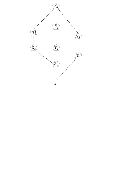
Figure 1: Basic $S_{4}$ subgroup structure. $S_{n}$ is the permutation symmetry of $n$ objects. $D_{4}$ is the dihedral group, while $V_{4}\sim Z_{2}\times Z_{2}$ is the Klein group.

In order to determine which of the above is the Galois group, we will examine partially symmetric polynomials of the roots of the corresponding equation (3.7). If we denote with $t_{i}$ the roots of the above polynomial, we know that any symmetric polynomial $f(t_{1},\dots,t_{4})$ can be written in terms of the quantities $s_{1}=\sum t_{i}=-a_{4}/a_{5},\dots,s_{4}=t_{1}t_{2}t_{3}t_{4}=a_{1}/a_{5}$ in a unique way. A partially symmetric function is left invariant only under a specific subgroup of $S_{4}$ and this defines the Galois group.

3.3 The $A_{4}$ case

In this section we will introduce appropriate partially symmetric functions of roots $t_{i}$ which remain invariant only under the desired $S_{4}$ subgroups. Then, for each particular case we will investigate the implications for the coefficients $a_{i}$.

We start the analysis with the discriminant $\Delta(t_{i})$ of the quartic polynomial which is of particular importance. This is a symmetric function of the roots $t_{i}$, written as follows

$$\Delta=\prod_{i\neq j}(t_{i}-t_{j})=\prod_{i<j}(t_{i}-t_{j})^{2}$$

and as such, remains invariant under the whole $S_{4}$ group. Now, we recall first that the $A_{4}$ discrete subgroup involves only the even permutations of $S_{4}$. If we take the quantity

$$\delta=(t_{1}-t_{2})(t_{1}-t_{3})(t_{1}-t_{4})(t_{2}-t_{3})(t_{2}-t_{4})(t_{3}-t_{4})$$

we can readily observe that this is invariant only under even permutations of roots. Observe now that $\delta$ is the square root of the discriminant of the polynomial related to ${\cal C}_{4}$

$$\Delta(t_{i})=\delta^{2}(t_{i})$$

We proceed now by examining the latter as functions of the coefficients $a_{k}$. As a symmetric function, the discriminant $\Delta$ is given in terms of the polynomial coefficients and is proportional to the Sylvester determinant given by

$$S_{d}=\left|\begin{array}[]{lllllll}a_{5}&a_{4}&a_{3}&a_{2}&a_{1}&0&0\\ 0&a_{5}&a_{4}&a_{3}&a_{2}&a_{1}&0\\ 0&0&a_{5}&a_{4}&a_{3}&a_{2}&a_{1}\\ 4a_{5}&3a_{4}&2a_{3}&a_{2}&0&0&0\\ 0&4a_{5}&3a_{4}&2a_{3}&a_{2}&0&0\\ 0&0&4a_{5}&3a_{4}&2a_{3}&a_{2}&0\\ 0&0&0&4a_{5}&3a_{4}&2a_{3}&a_{2}\end{array}\right|$$ (3.8)

while $S_{d}=a_{5}\Delta$. Substituting the $b_{1}=0$ conditions found in (3.4) for the upper signs, $S_{d}$ takes the form

$$\begin{split}S_{d}=&a_{7}a_{0}^{2}\left(27a_{7}^{2}a_{0}a_{2}^{4}+2a_{6}a_{0}\left(2a_{0}a_{6}^{2}+9a_{3}a_{7}\right)a_{2}^{3}\right.\\ &\left.-\left(4a_{7}a_{3}^{3}+\left(a_{3}a_{6}^{2}+144a_{1}a_{7}^{2}\right)a_{0}a_{3}+6a_{1}a_{6}^{2}a_{7}a_{0}^{2}\right)a_{2}^{2}\right.\\ &\left.+2a_{1}a_{6}a_{0}\left(-40a_{7}a_{3}^{2}-9a_{6}^{2}a_{0}a_{3}+96a_{1}a_{7}^{2}a_{0}\right)a_{2}\right.\\ &\left.+a_{1}\left(16a_{7}a_{3}^{4}+4\left(a_{3}a_{6}^{2}+32a_{1}a_{7}^{2}\right)a_{0}a_{3}^{2}+27a_{1}a_{6}^{4}a_{0}^{3}\right.\right.\\ &+\left.\left.16a_{1}a_{7}\left(9a_{3}a_{6}^{2}+16a_{1}a_{7}^{2}\right)a_{0}^{2}\right)\right)\end{split}$$ (3.9)

The form of the discriminant for the lower signs of (3.4) is derived by just substituting $a_{0}\to-a_{0}$. For arbitrary $a_{i}$’s (more precisely imposing no other condition on $a_{i}$’s), in general the discriminant cannot be written as a square of a quantity with all elements in ${\cal F}$. Then, the Galois group is $S_{4}$ or one of the subgroups $D_{4},Z_{4}$. If the discriminant is a square of a quantity $\delta$ then the Galois group is $A_{4}$ or $V_{4}=Z_{2}\times Z_{2}$.

3.4 The $\Delta=\delta^{2}$ constraints on $a_{k}$’s

We will attempt to unravel possible relations of the $a_{i}$ coefficients for the case of the $A_{4}$ symmetry. Undoubtedly, the relevant condition $\Delta=\delta^{2}$ could be met only for very particular relations among $a_{k}$. The search for any correlations however, is not a trivial task, given the complicated form of (3.9).

We choose to proceed with this investigation as follows: If we consider $\Delta$ as a polynomial of a certain $a_{k}$ coefficient ($k=1,...,5$), i.e.,

$$\Delta\to f(a_{k})=c_{n}a_{k}^{n}+\cdots+c_{0},\;\;n\leq 4$$

a necessary condition for $\Delta$ to be written as a square is the vanishing of the discriminant of the polynomial $f(a_{k})$. There are 5 such coefficients, hence there are an equal number of choices. To choose a suitable case, we expand the discriminant in each of the available coefficients. We obtain

$$\Delta=\left\{\begin{array}[]{ll}f_{5}&=0\,{\bf a_{5}^{4}}+256a_{1}^{3}{\bf a_{5}^{3}}+\cdots\\ f_{4}&=-27a_{1}^{2}{\bf a_{4}^{4}}+\cdots\\ f_{3}&=16a_{1}a_{5}{\bf a_{3}^{4}}+\cdots\\ f_{2}&=-27a_{5}^{2}{\bf a_{2}^{4}}+\cdots\\ f_{1}&=0\,{\bf a_{1}^{4}}+256a_{5}^{3}{\bf a_{1}^{3}}+\cdots\end{array}\right.$$ (3.10)

From these five expansions we see that in two cases ($f_{1},f_{5}$), $\Delta$ can be expressed as a third order polynomial whilst in the three remaining cases it is a polynomial of fourth degree. A necessary condition to write the third degree polynomials as a square is that the coefficient of the highest (third) degree is positive definite, i.e. ${\rm sign}(a_{1}a_{5})=(+)$. As far as the fourth degree ones are concerned, this criterion is fulfilled only for $f_{3}$, provided the same condition holds, i.e. ${\rm sign}(a_{1}a_{5})=(+)$. The highest degree coefficients of the other two fourth-degree polynomials $f_{2},f_{4}$ cannot be positive definite and as such they are automatically rejected.

There is an advantage of the fourth degree polynomial since when the required criteria are satisfied this can be a product of two second degree ones, and it is possibly more convenient to handle them.

Under these circumstances, the only case to satisfy the requiring criteria is when we consider $\Delta$ as a polynomial with respect to $a_{3}$ , i.e,

$$\Delta\to f_{3}(a_{3})=c_{4}a_{3}^{4}+c_{3}a_{3}^{3}+c_{2}a_{3}^{2}+c_{1}a_{3}+c_{0}$$

where all $c_{k}$ are known functions of $a_{i}$. Computing the discriminant of $f_{3}$ , we find that it is proportional to $\Delta_{f_{3}}\propto D_{a}^{2}D_{b}^{3}$ with

$$\begin{split}D_{a}&=a_{1}a_{4}^{2}-a_{2}^{2}a_{5}\\ D_{b}&=\left(27a_{1}^{2}a_{4}-a_{2}^{3}\right)a_{4}^{3}-6a_{1}a_{2}^{2}a_{5}a_{4}^{2}+4096a_{1}^{3}a_{5}^{3}+3a_{2}\left(9a_{2}^{3}-256a_{1}^{2}a_{4}\right)a_{5}^{2}\end{split}$$ (3.11)

As we have pointed out, a necessary condition to write $\Delta=\delta^{2}$ is the vanishing of the discriminant $\Delta_{f_{3}}$ of the polynomial $f_{3}$. There are two ways to satisfy this constraint, either by setting $D_{a}=0$ or for $D_{b}=0$. With a detailed discussion given in the Appendix, we record here the induced conditions among the coefficients. From $D_{a}=0$ we readily see that

$$a_{1}a_{4}^{2}=a_{2}^{2}a_{5}$$ (3.12)

As explained in the Appendix, this condition is not sufficient to write $\Delta=\delta^{2}$. This happens if we require

$$a_{2}^{2}=2\,a_{1}\,a_{3},\;a_{4}^{2}=2\,a_{3}\,a_{5}$$ (3.13)

From the second $D_{b}=0$, after several algebraic manipulations we end up with the condition

$$(a_{2}^{2}a_{5}-a_{4}^{2}a_{1})^{2} = \left(\frac{16a_{1}a_{5}-a_{2}a_{4}}{3}\right)^{3}$$ (3.14)

Plugging in the above the $SU(5)$ constraint $b_{1}=0$ yields

$$(a_{2}^{2}a_{7}-a_{0}a_{1}a_{6}^{2})^{2} = a_{0}\left(\frac{16a_{1}a_{7}+a_{2}a_{6}}{3}\right)^{3}$$ (3.15)

As it is expected, such relations will have also implications on the matter curves. Thus, from the first condition in particular we find that the fiveplets split to three orbits according to

$$P_{5}=a_{6}(2a_{0}a_{1}a_{6}-a_{2}a_{3})\left(a_{3}a_{6}^{2}+\left(a_{2}a_{6}+a_{1}a_{7}\right)a_{7}\right)$$ (3.16)

with their homologies computed directly from those of $a_{i}$’s given in Table  1.

3.4.1 The spectrum of the $SU(5)\times A_{4}\times U(1)$ model

In this section we present the $SU(5)$ spectrum subject to the constraints of the $A_{4}$ monodromy. In order to clarify its properties we find it convenient to change the notation with respect to $t_{1,\dots,4}$-roots in an $A_{4}$ basis. To this end, we recall that the permutations of the four roots $t_{1,2,3,4}$ constitute the $S_{4}$ group while their sum

$$t_{s}=t_{1}+t_{2}+t_{3}+t_{4}$$

clearly remains invariant under all permutations. This is orthogonal to the three remaining combinations

$$t_{a}=t_{1}+t_{2}-t_{3}-t_{4},\;t_{b}=t_{1}-t_{2}+t_{3}-t_{4},\;t_{c}=t_{1}-t_{2}-t_{3}+t_{4}$$

which form an $S_{4}$-triplet. The action of only $S_{4}$-even permutations of roots ( $Q_{even}$) , corresponds to the $A_{4}$ subgroup. Under these permutations we see that

$$Q_{even}t_{\gamma}=\pm t_{\delta},\;(\gamma,\delta)\in(a,b,c)$$

From equations (3.6) of the tenplets we can see that those corresponding to the four roots $t_{1,2,3,4}$ are associated to $a_{1}$. These can be expressed as a singlet and a triplet under $S_{4}/A_{4}$ as follows

$$\Sigma_{10_{1}}:\;(10,1)=10_{t_{s}},\;\Sigma_{10_{3}}:\;(10,3)=\{10_{t_{a}},10_{t_{b}},10_{t_{c}}\}$$

This means that $P_{10}$ should split to three factors which essentially requires $a_{1}$ to be the product of two factors $a_{1}\sim\beta_{0}\beta_{1}$.

We turn now our attention to the fiveplets. In the new basis $t_{s,a,b,c}$, the $\bar{5}_{t_{i}+t_{j}}$’s are written as $t_{s}\pm t_{\gamma}$, with $\gamma=a,b,c$ and similarly for the $5$’s defined by $-(t_{i}+t_{j})$ . Thus, this subset of $SU(5)$ multiplets form two triplets under $A_{4}$ , namely

$$3_{\pm}=\frac{1}{2}(t_{s}\pm t_{a,b,c})$$

whose components are interchanged by the action of $A_{4}$, i.e., $Q_{even}:3_{+}\to 3_{-}$. The corresponding matter curves accommodate the elements

$$(5,3)_{(\pm)}=(5_{\frac{1}{2}(t_{s}\pm t_{a})},\,5_{\frac{1}{2}(t_{s}\pm t_{b})},\,5_{\frac{1}{2}(t_{s}\pm t_{c})})$$

In the new ‘basis’ the elements $5_{t_{i}+t_{5}}$ form a singlet and a triplet, i.e.

$$5_{t_{1}+t_{5}}\to 5_{\frac{1}{4}(t_{s}+t_{a}+t_{b}+t_{c})+t_{5}},$$

and

$$(5_{t_{2}+t_{5}},5_{t_{3}+t_{5}},5_{t_{4}+t_{5}})\to(5_{\frac{1}{4}(t_{s}+t_{a}-t_{b}-t_{c})+t_{5}},5_{\frac{1}{4}(t_{s}-t_{a}+t_{b}-t_{c})+t_{5}},5_{\frac{1}{4}(t_{s}-t_{a}-t_{b}+t_{c})+t_{5}})$$

We also need to rewrite the $t_{i}-t_{j}$ differences in the new basis, for the classification of the $SU(5)$ singlets. These can be expressed as $t_{i}-t_{j}=t_{\gamma}-t_{\delta}$ for ${\gamma,\delta}=a,b,c$. Accordingly, for $t_{i}-t_{5}$ we have a singlet $\theta_{0}=(1,1)_{-t_{5}}$ and a triplet $\theta_{3}=(1,3)_{-t_{5}}$ in analogy with the fiveplets $\bar{5}_{t_{i}+t_{5}}$ above. All representations are collected and assigned under the new notation in Table 3.

Curve	$SU(5)\times A_{4}\times U(1)$	$t_{\gamma}$	$matter$
$\Sigma_{10_{a}}:$	$F=(10,3)$	${t_{a}}$	$F_{i}=(Q,u^{c},e^{c})_{i}$
$\Sigma_{10_{b}}:$	$F_{x}=(10,1)$	${t_{s}}$
$\Sigma_{10_{c}}:$	$F_{y}=(\overline{10},1)_{-t_{5}}$	${-t_{5}}$
$\Sigma_{5_{1}}:$	$H=\bar{(}5,3)$	${t_{s}\pm t_{a}}$	$h_{u}$
$\Sigma_{5_{2}}:$	$\bar{f}=(\bar{5},3)_{+t_{5}}$	${\frac{1}{4}(t_{s}-t_{a})+t_{5}}$	$\bar{f}_{i}=(\ell,d^{c})_{i}$
$\Sigma_{5_{3}}:$	$\bar{H}=(\bar{5},1)_{+t_{5}}$	$\frac{1}{4}(t_{s}+3t_{a})+t_{5}$	$\bar{h}_{d}$
$\Sigma_{1_{a}}:$	$\theta_{a}=(1,3)$	0	$\theta_{ij}$
$\Sigma_{1_{b}}:$	$\theta_{b}=(1,3)$	$t_{a}$	$\theta_{i4}$
$\Sigma_{1_{c}}:$	$\theta_{c}=(1,3)_{-t_{5}}$	${\frac{1}{4}(t_{s}-t_{a})-t_{5}}$	$\theta_{i5}$
$\Sigma_{1^{\prime}}:$	$\theta^{\prime}=(1,1)_{-t_{5}}$	$-t_{5}$	$\theta_{45}$
$\Sigma_{1^{\prime\prime}}:$	$\theta^{\prime\prime}=(1,1)_{+t_{5}}$	$t_{5}$	$\theta_{54}$
$\Sigma_{1_{0}}:$	$\theta=(1,1)$	$0$	$\theta$

Table 3: Field representation content for the $SU(5)\times A_{4}\times U(1)$ case 1. For alternative models, matter resides on $\Sigma_{10_{b,c}}$ curves (see text).

3.5 Further reduction of the discrete group

We will examine the conditions on $a_{k}$ coefficients to reduce the $S_{4}/A_{4}$ down to their subgroups (we follow closely the notations of [29]). Given the property of the discriminant, (i.e whether it is a square root or not) we may have a different symmetry breaking chain. We have seen what we should expect an $A_{4}$ discrete group (or its subgroup $V_{4}$) if $\Delta=\delta^{2}$. On the contrary, if $\Delta\neq\delta^{2}$ we will see that the Galois group is $S_{4}$ or $D_{4},Z_{4}$. To check this we need to examine other partially symmetric functions of roots. To this end, consider the sums 

$$x_{1}=t_{1}t_{2}+t_{3}t_{4},\;x_{2}=t_{1}t_{3}+t_{2}t_{4},\;x_{3}=t_{3}t_{2}+t_{1}t_{4},$$

To construct an appropriate function of $t_{i}$, we assume the associated cubic polynomial (the resolvent of ${\cal P}_{4}(s)$) with roots the $x_{1,2,3}$

$$f(x)=(x-x_{1})(x-x_{2})(x-x_{3})$$ (3.17)

This is invariant under $S_{4}$ and has the same discriminant as ${\cal P}_{4}(s)$.

We examine here a partially symmetric quantity (function of roots) which is invariant under the Dihedral subgroup $D_{4}$. This is the sum

$$x_{1}=t_{1}t_{2}+t_{3}t_{4}$$

This remains unaltered by the following eight $S_{4}$ elements

$$I,(12),(34),(12)(34),(14)(23),(13)(24),(1423),(1324)$$

This is one of the three dihedral subgroups $D_{4}$ of $S_{4}$. Similarly we work for the other two quantities $x_{2,3}$ each remaining invariant under the appropriate dihedral subgroup $D_{4}$ (see table 4).

$D_{a}$	$I,(12),(34),(12)(34),(14)(23),(13)(24),(1423),(1324)$	$t_{1}t_{2}+t_{3}t_{4}$
$D_{b}$	$I,(13),(24),(12)(34),(14)(23),(13)(24),(1234),(1432)$	$t_{1}t_{3}+t_{2}t_{4}$
$D_{c}$	$I,(14),(23),(12)(34),(14)(23),(13)(24),(1243),(1342)$	$t_{1}t_{4}+t_{2}t_{3}$

Table 4: The three Dihedral groups isomorphic to $D_{4}$ and their invariants.

The symmetry splits the fiveplets in three orbits according to

$$R_{a}=\{t_{1}+t_{2},\,t_{3}+t_{4}\},\;R_{b}=\{t_{1}+t_{3},\,t_{2}+t_{4}\},\;R_{c}=\{t_{1}+t_{4},\,t_{2}+t_{3}\},$$ (3.18)

The coefficients of $f(x)$ can be computed as functions of $a_{k}$. In particular, the $S_{4}$ invariant quantity

$$f(0)=x_{1}x_{2}x_{3}=(t_{1}t_{2}+t_{3}t_{4})(t_{1}t_{3}+t_{2}t_{4})(t_{3}t_{2}+t_{1}t_{4})$$

is expressed in terms of $a_{k}$’s as follows

$$f(0)=4a_{5}a_{3}a_{1}-a_{4}^{2}a_{1}-a_{5}a_{2}^{2}$$ (3.19)

Substitution of the conditions for $b_{1}=0$ transform the above to

$$f(0)=\alpha_{0}\left(a_{2}^{2}a_{7}-a_{1}\left(\alpha_{0}a_{6}^{2}+4a_{3}a_{7}\right)\right)$$

If the polynomial is irreducible, then $f(0)\neq 0$. This, and the condition $\Delta\neq\delta^{2}$ imply that the group is $S_{4}$.

Now let’s examine the case of a reducible $f(x)$. The polynomial $f(x)$ can be factorised for $f(0)=0$

$$f(x)=x^{3}+f_{1}x^{2}+f_{2}x=x(x^{2}+f_{1}x+f_{2})$$

This yields

$$a_{2}^{2}a_{7}=a_{1}\left(\alpha_{0}a_{6}^{2}+4a_{3}a_{7}\right)$$

Substitution of the latter into the equation of fiveplets gives

$$P_{5}=a_{3}\left(a_{2}a_{6}+4a_{1}a_{7}\right)\left(a_{3}a_{6}^{2}+a_{7}\left(a_{2}a_{6}+a_{1}a_{7}\right)\right)$$

Therefore, for the case of dihedral symmetry $D_{4}$ the fivelpets split to three orbits with homologies

$$[a_{3}]=\eta-3c_{1}-\chi,\;\;[a_{2}a_{6}]=\eta-4c_{1},\;\;[a_{2}a_{6}a_{7}]=\eta-3c_{1}+\chi$$

Finally, notice that the substitution of equations (3.13) to (3.19) automatically implies $f(0)=0$ thus these are just the requirements for the symmetry reduction down to $V_{4}\sim Z_{2}\times Z_{2}$.

The present analysis with respect to $\Delta$ and $f(x)$ is summarised in Table 5.

Discriminant	$f(x)$	Group
$\Delta\neq\delta^{2}$	$f(0)\neq 0\;$:	$S_{4}$
	$f(0)=0\;$:	$D_{4}$
$\Delta=\delta^{2}$	$f(0)\neq 0\;$:	$A_{4}$
	$f(0)=0\;$:	$V_{4}$

Table 5: The Galois groups for the various cases of the Discriminant and the reducibility of the resolvent cubic $f(x)=(x-x_{1})(x-x_{2})(x-x_{3})$ in (3.17).

3.6 Embedding of $A_{4}$ models in the $SU(4)$ spectral cover

Among other cases discussed in the previous sections, we have also derived the constraints on the coefficients $a_{i}$ for which the monodromy group reduces to $A_{4}$. In this case, we find it useful to determine the embedding of the fields $10_{t_{a}},\bar{5}_{t_{a}+t_{b}}$ etc in $A_{4}$ representations.

We can proceed as follows: having in mind the particular splitting of the spectral cover we are dealing with in this work, i.e. ${\cal C}_{4}\times{\cal C}_{1}$, for our present purposes we may consider the $SU(4)$ as the covering group of the monodromy and the embedding of the fields into its $4$ and $6$ representations. Indeed, recall that ${E}_{8}\supset SO(10)\times SU(4)$ while matter resides in the ${E}_{8}$ adjoint representation 248, which in this case decomposes as follows

${248}\;\rightarrow\;(45,1)+(\overline{16},{\bar{4}_{\perp}})+$$(16,{4_{\perp}})+(10,{6_{\perp}})+(1,{15_{\perp}})$

The relevant -w.r.t. ordinary matter- representations are included in the box. $16^{\prime}s$ and $10^{\prime}s$ include the non-trivial $SU(5)$ representations while $(1,{15_{\perp}})$ is an $SU(5)_{GUT}$ singlet.

As demonstrated in [30], the $A_{4}$ representations are in one-to-one correspondence with those of $SU(3)$, thus the $SU(4)$ ones decompose according to the pattern shown in Table 6.

$SU(4)$	$SU(3)$	$A_{4}$
$4$	$3+1$	$3+1$
$6$	$3+\bar{3}$	$3$
$15$	$8+1+3+\bar{3}$	$3+3^{\prime}+1+1^{\prime}+1^{\prime\prime}$

Table 6: Decomposition of the ${\cal C}_{4}$ spectral cover symmetry to $A_{4}$

In this case the spectrum emerges according to the chain rules

$$\begin{split}(16,4)&\stackrel{{\scriptstyle\rm SO(10)\times SU(3)}}{{\longrightarrow}}(16,3)+(16,1)\\ &\stackrel{{\scriptstyle\rm SU(5)\times A_{4}}}{{\longrightarrow}}[(10,3)+(\bar{5},3)+(1,3)]+[[(10,1)+(\bar{5},1)+(1,1)]\\ (10,6)&\stackrel{{\scriptstyle\rm SO(10)\times SU(3)}}{{\longrightarrow}}(10,3)+(10,\bar{3})\\ &\stackrel{{\scriptstyle\rm SU(5)\times A_{4}}}{{\longrightarrow}}(5,3)+(\bar{5},3)\\ (1,15)&\stackrel{{\scriptstyle\rm SO(10)\times SU(3)}}{{\longrightarrow}}(8+1+3+\bar{3})\\ &\stackrel{{\scriptstyle\rm SU(5)\times A_{4}}}{{\longrightarrow}}(1,3)+(1,3^{\prime})+1+1^{\prime}+1^{\prime\prime}\end{split}$$ (3.20)

These results are in accordance with the analysis of our previous sections. In the next section, we will work out a few examples of effective models paying attention to the neutrino sector.

4 Effective low energy theory

In this section we seek to build effective low energy models which incorporate the discrete symmetries analysed above. Motivated by the successful implementation of the $A_{4}$ in the neutrino sector, we will mainly focus in this case and its subgroups.

4.1 Neutrino masses from $A_{4}$

Observing the spectrum presented in Table 3, we notice that there are more than one ways to accommodate the generations on matter curves. We present these possibilities starting with the charged sector.

4.1.1 Case 1

Taking the point of view that three of the tenplets are accommodated as an $A_{4}$-triplet, as a first example, we choose to accommodate the three families of quark doublets etc, in $(10,3)$ since in this context it is the only possible way to obtain a tree-level top-quark coupling. We notice however that in this case it is not obvious how to generate chirality for the $SU(5)$ representations. In this case we envisage that in the yet unspecified global geometrical structure, higher dimensional non-Abelian internal fluxes will restrict non-trivially on the $\Sigma_{(10,3)}$ matter curve inducing a chiral spectrum sitting in $(10,3)$. There is a second shortcoming in this picture which will be revealed as soon as we write down the charged fermion mass terms.

We start by making the assignment for the remaining SM fermions and Higgs according to Table 3. Then the following couplings emerge

$$\begin{split}{\cal W}_{u}&\supset\;(10,3)_{t_{i}}\,(10,3)_{t_{i}}\,(5,3)_{-2t_{i}}\\ {\cal W}_{d,\ell}&\supset\;(10,3)_{t_{i}}\,(\bar{5},3)_{t_{i}+t_{5}}\,(\bar{5},1)_{t_{4}+t_{5}}\theta_{i5}\\ {\cal W}_{\nu}&\supset\;(\bar{5},3)_{t_{i}+t_{5}}\,(\bar{5},3)_{t_{i}+t_{5}}\,(5,3)_{-2t_{i}}\,(5,3)_{-2t_{i}}\theta_{i5}\theta_{i5}\\ \end{split}$$ (4.1)

Recall that the $A_{4}$ tensor products are

$$3\times 3\to 1+1^{\prime}+1^{\prime\prime}+3_{s}+3_{a},\;1^{\prime}\times 1^{\prime\prime}\to 1$$

Notice that the up-Higgs fiveplet is also an $A_{4}$ triplet. The most general vev can be written

$$h_{u}=(h_{1},h_{2},h_{3}),\;\to\;\langle h_{u}\rangle=(v_{1},v_{2},v_{3})$$

For the up quarks we get

$$\begin{split}F\,F\,h_{u}&=(2F_{1}F_{1}-F_{2}F_{3}-F_{3}F_{2})\,v_{1}\\ &+(2F_{3}F_{3}-F_{1}F_{2}-F_{2}F_{1})\,v_{3}\\ &+(2F_{2}F_{2}-F_{1}F_{3}-F_{3}F_{1})\,v_{2}\\ \end{split}$$ (4.2)

Then, to first order, the matrix for the up quarks is

$$m_{u}=\left(\begin{array}[c]{ccc}2v_{1}&-v_{3}&-v_{2}\\ -v_{3}&2v_{2}&-v_{1}\\ -v_{2}&-v_{1}&2v_{3}\end{array}\right)$$

For the leptons one gets

$$\begin{split}F\,\bar{f}\,\bar{H}\,\theta_{i5}&=(10,3)_{t_{i}}(\bar{5},3)_{t_{i}+t_{5}}(\bar{5},1)_{t_{4}+t_{5}}\theta_{i5}\end{split}$$ (4.3)

The $SU(5)$ singlets $\theta_{ab}$ participating in this coupling compose an $A_{4}$-triplet. Assuming the triplet vev $\langle\theta_{ab}\rangle\sim(a_{1},a_{2},a_{3})$, in this case we get

$$m_{\ell}\sim\left(\begin{array}[]{lll}2a_{1}&-a_{3}&-a_{2}\\ -a_{3}&2a_{2}&-a_{1}\\ -a_{2}&-a_{1}&2a_{3}\end{array}\right)\,\langle h_{d}\rangle$$

The down quarks and charged leptons look identical, however, in general radiate effects are expected to discriminate them.

We observe that there is a generic structure of tree-level masses for the charged fermions’ sector. Hence, in both cases, the eigenvalues are given by common formulae, satisfying the sum rule

$$m_{3}=m_{1}+{m_{2}}=\sum_{i}a_{i}$$

Apparently, this cannot be satisfied by any mass relations of quarks and/or charged leptons. Higher order corrections cannot make this compatible with data, therefore, the present assignment appears to be too restrictive. We proceed to an alternative scenario.

4.1.2 Case 2

To avoid the problem with the charged fermion sector we assume that the 10 representation of $SU(5)$ accommodating the left handed doublet quarks of the three families is an $A_{4}$ singlet. We may use either of the two matter curves $\Sigma_{10_{b,c}}$ to accommodate the three families. For example, if we assign

$$F_{x}=(10,1)=(Q,d^{c}e^{c})$$

then, for the up quarks the allowed coupling is the following fourth order one

$$\lambda_{t}\frac{1}{\Lambda}\,(10,1)\,(10,1)\,(5,3)\,(1,3)\leftrightarrow\lambda_{t}\frac{1}{\Lambda}\,F_{x}F_{x}H\theta_{b}$$

Assigning $\langle H\rangle=(v_{1},v_{2},v_{3}),\langle\theta_{b}\rangle=(b_{1},b_{2},b_{3})$, this induces a mass for the third generation up quark

$$m_{t}\sim\lambda_{t}\frac{v_{1}b_{1}+v_{2}b_{3}+b_{3}v_{2}}{\Lambda}$$

If all families are on the same matter curve, according to [10, 11] the lighter generations receive masses from non-commutative fluxes and instanton effects.

For down quarks and leptons we can write a fifth order coupling

$$\frac{1}{\Lambda^{2}}(10,1)\,(\bar{5},3)_{t_{5}}\,(\bar{5},1)_{t_{5}}\,(1,3)_{-t_{5}}^{2}\leftrightarrow\frac{1}{\Lambda^{2}}F_{x}f\bar{H}\theta_{c}^{2}$$

with a mass eigenvalue associated to the bottom quark

$$m_{b}\sim\lambda_{b}\frac{\langle\theta_{c}^{2}\rangle}{\Lambda^{2}}\,\langle h_{d}\rangle$$

In this scenario, non-perturbative corrections and non-commutative fluxes are expected to generate the lighter masses.

As an alternative possibility, we mention that families may also reside on $\Sigma_{10_{c}}$. The corresponding representations $10_{t_{5}}$ are charged under the $U(1)_{t_{5}}$ factor. As a consequence, chirality is readily obtained by turning on appropriate $U(1)$ flux along $t_{5}$, however the disadvantage here is that the top Yukawa coupling arises only at sixth order.

4.1.3 Neutrinos

We turn now our attention to the couplings of the neutrinos. There is an effective Majorana operator at sixth order

$${\cal W}_{\nu}=\bar{f}\cdot\bar{f}\,\cdot\bar{H}\cdot\bar{H}\,\cdot\theta_{i5}\cdot\theta_{i5}$$

Inasmuch the involved fields are triplets under the $A_{4}$ symmetry, there are various ways to obtain $A_{4}$ invariants. Notice first

$$\begin{split}\bar{f}\cdot\bar{f}\to 3\times 3&=1_{f}+1_{f}^{\prime}+1_{f}^{\prime\prime}+3_{f}+3_{f}^{\prime}\\ \bar{H}\cdot\bar{H}\to 3\times 3&=1_{h}+1_{h}^{\prime}+1_{h}^{\prime\prime}+3_{h}+3_{h}^{\prime}\\ \theta_{i5}\cdot\theta_{i5}\to 3\times 3&=1_{\theta}+1_{\theta}^{\prime}+1_{\theta}^{\prime\prime}+3_{\theta}+3_{\theta}^{\prime}\end{split}$$ (4.4)

Hence, we have several $A_{4}$ invariants contributing to $m_{\nu}$ such as

$$\begin{split}m_{\nu}&\propto 1_{\theta}(1_{f}1_{h}+1_{f}^{\prime}1_{h}^{\prime\prime}+1_{f}^{\prime\prime}1_{h}^{\prime})\\ &+1_{\theta}^{\prime}(1_{f}1_{h}^{\prime\prime}+1_{f}^{\prime\prime}1_{h}+1_{f}^{\prime}1_{h}^{\prime})\\ &+1_{\theta}^{\prime\prime}(1_{f}1_{h}^{\prime}+1_{f}^{\prime\prime}1_{h}+1_{f}^{\prime\prime}1_{h}^{\prime\prime})\\ &+1_{\theta}\cdot(3_{f}\times 3_{h})_{1}+\cdots\end{split}$$ (4.5)

With the above analysis at hand, we proceed now to a simple example. We would like to see whether at a first approximation the specified neutrino mass structure is in accordance with large mixing as indicated by the experimental data. Therefore, we take a toy example and choose the vev alignments to be

$$\left\{a_{1}\to 1,a_{2}\to 0,a_{3}\to 0,v_{1}\to 0,v_{3}\to v_{2}\right\}$$

If we assign with $V_{\ell}$ the unitary matrix diagonalising the charged lepton sector and $V_{\nu}$ the corresponding one for the neutrino mass matrix, the lepton mixing matrix to be compared with the experiment is the product $V=V_{\ell}^{\dagger}V_{\nu}$. In the case of the charged leptonic sector discussed previously, the structure of the mass matrix is generated by non-perturbative contributions and the mixing effects are expected to be small. In this case the large mixing effects measured in the neutrino experiments are generated by $V_{\nu}$. In the present model, the neutrino mass matrix takes the form

$$m_{\nu}\propto\left(\begin{array}[]{lll}2&1\cdot c&1\cdot c\\ 1\cdot c&13&-4\cdot c\\ 1\cdot c&-4\cdot c&13\end{array}\right)$$

In the above texture we have inserted an arbitrary coefficient $c$ to parametrise corrections from the charged lepton sector and renormalisation effects. This is a simplified approximation, however at present we would like to show that the observed large mixing effects arise indeed from the neutral sector of the theory. Hence, the choice $c=2$ yields

$$V_{\nu}=\left(\begin{array}[]{lll}-0.85689&0.515499&0.\\ 0.364513&0.605913&-0.707107\\ 0.364513&0.605913&0.707107\end{array}\right)$$ (4.6)

Although in this simplified procedure the prediction for the $\theta_{13}$ mixing angle turns out to be strictly zero, even small charged lepton mixing will lift this to a non-zero value, hopefully compatible with data. Undoubtedly, it is remarkable that in general the mixing angles are pretty close to the measured values. The eigenmasses are

$$V_{\nu}^{\dagger}m_{\nu}V_{\nu}\;\to\;\left(0.3,6.7,21.0\right)\,m_{0}$$

predicting a ratio $r=\Delta m_{atm}^{2}/\Delta m_{sun}^{2}\approx 10$. This value is not far from from the experimental one ($r\sim 30$). Nevertheless, a more detailed investigation should take into account renormalisation group effects which are beyond the purpose of the present work.

4.2 ${Z}_{2}\times{Z}_{2}$ Models

In recent attempts to interpret the neutrino data in the context of field theory models, a wide number of other (simpler) discrete symmetries have also been proposed. Motivated by these attempts in this section we will examine neutrino mass textures which are derived only from combinations of ${Z}_{n}$ symmetries. Based on the analysis of previous works on F-theory models, here we will derive the neutrino mass textures for the ${Z}_{2}\times{Z}_{2}$ case. In conjunction with our previous analysis, this may arise under the following braking chain

$$SU(5)_{\perp}\to SU(4)\to A_{4}\to{Z}_{2}\times{Z}_{2}$$

$SU(5)$	$U(1)$ “weight”	homology	$U(1)_{Y}$	$U(1)_{X}$
$10^{(1)}$	$\pm{t_{1,2}}$	$\eta-2c_{1}-{\chi}-\psi$	$N_{1}$	$M_{10}^{1}$
$10^{(2)}$	$\pm{t_{3}}$	$-2c_{1}+\chi$	$N_{2}$	$M_{10}^{2}$
$5^{(0)}$	$\mp({t_{1}+t_{2}})$	$-c_{1}+{\chi}+\psi$	$-N_{1}$	$M_{5}^{0}$
$5^{(1)}$	$\mp({t_{1,2}+t_{3}})$	$2\eta-4c_{1}-2{\chi}-2\psi$	$2N_{1}$	$M_{5}^{1}$
$5^{(2)}$	$\mp({t_{1,2}+t_{5}})$	$\eta-2c_{1}-{\chi}-\psi$	$N_{1}$	$M_{5}^{2}$
$5^{(3)}$	$\mp({t_{3,4}+t_{5}})$	$-2c_{1}+{\chi}+2\psi$	$-2N_{1}-N_{2}$	$M_{5}^{3}$
$5^{(4)}$	$\mp({t_{3}+t_{4}})$	$-c_{1}+\chi$	$N_{2}$	$M_{5}^{4}$
$10^{{(3)}}$	$\pm{t_{5}}$	$-c_{1}+\psi$	$-N_{1}-N_{2}$	$M_{10}^{3}$

Table 7: $SU(5)$ matter curves, their homology class and the $U(1)_{X,Y}$ flux parameters for the ${Z}_{2}\times{Z}_{2}$ case. The signs $\pm t_{i}$ are associated to $10/\overline{10}$ representation accommodated on the specific matter curve, while $\mp(t_{i}+t_{j})$ to $5/\bar{5}$ ones.

4.2.1 $SU(5)$ spectrum

In the $SU(5)$ model with ${Z}_{2}\times{Z}_{2}$ discrete symmetry, the spectral cover equation for $SU(5)_{\perp}$ is written in the form

$${\cal C}_{5}(s) = \left(a_{3}s^{2}+a_{2}s+a_{1}\right)\left(a_{6}s^{2}+a_{5}s+a_{4}\right)(a_{7}+a_{8}s)$$ (4.7)

Proceeding as above, we start by identifying the relations $b_{k}(a_{i}),k=1,\dots 5$ by comparing coefficients of the same power in $s$ of the polynomials (2.2) and (4.7).

The $10\in SU(5)$ are in one to one correspondence with the solutions of the equation

$$b_{5}=a_{1}a_{4}a_{7}=0$$

therefore they are associated to $a_{1}=0,a_{4}=0$ and $a_{7}=0$. The fiveplets are found by solving the corresponding equation (3.5) which in terms of the $a_{i}$’s in the present case can be written [15, 19]:

$$\begin{split}P_{5}&=(a_{6}a_{7}+a_{5}a_{8})\times(a_{1}^{2}-a_{1}(a_{5}a_{7}+2a_{4}a_{8})\lambda+a_{4}(a_{6}a_{7}^{2}+a_{8}(a_{5}a_{7}+a_{4}a_{8}))\lambda^{2})\\ &\times(a_{1}-a_{5}a_{7}\lambda)\times(a_{6}a_{7}^{2}+a_{8}(a_{5}a_{7}+a_{4}a_{8}))\times a_{5}\end{split}$$ (4.8)

This equation has five factors corresponding to an equal number of fiveplets dubbed as

$$5^{(0)},5^{(1)},5^{(2)},5^{(3)},5^{(4)}$$

in the order of appearance in the product (4.8). It is straightforward to determine their homology classes, while to compute the flux restrictions we define

$${\cal F}_{Y}\cdot{\psi}=-N_{1}-N_{2},\;{\cal F}_{Y}\cdot{\chi}=N_{2},\;{\cal F}_{Y}\cdot\eta={\cal F}_{Y}\cdot c_{1}=0$$

where $N_{1,2}$ integers and ${\cal F}_{Y}$ the hypercharge flux.

The results are summarised in Table 7. In the first column we write the $SU(5)$ representation with a superscript denoting the specific matter curve. In the second column we write the corresponding $SU(5)_{\perp}$ root. The third column shows the homology classes of the matter curves computed in [15, 19]. The last two columns show the integers $N_{i},M_{j}$ associated to hypercharge and $U(1)_{X}$ fluxes respectively. The latter are subject to the restriction $\sum_{j}M_{j}=0$ [15].

We proceed with a specific example, based on the particular choice of fluxes $N_{1}=0,N_{2}=1$. For a given matter curve $\Sigma_{10}$ with $M_{10},N_{Y}$ units of $U(1)_{X}\in SU(5)_{\perp}$ and $U(1)_{Y}$ fluxes correspondingly, the multiplicities of the resulting SM spectrum are given by

$${\bf 10}\in SU(5)\Rightarrow\left\{\begin{array}[]{lll}n_{(3,2)_{\frac{1}{6}}}-n_{(\bar{3},2)_{-\frac{1}{6}}}&=&{M_{10}}\\ n_{(\bar{3},1)_{-\frac{2}{3}}}-n_{(3,1)_{\frac{2}{3}}}&=&{M_{10}}-{N_{Y}}\\ n_{(1,1)_{1}}-n_{(1,1)_{-1}}&=&{M_{10}}+{N_{Y}}\end{array}\right.$$ (4.12)

Similarly, for the $\Sigma_{5}$ curves

$${\bf 5}\in SU(5)\Rightarrow\left\{\begin{array}[]{lll}n_{(3,1)_{-\frac{1}{3}}}-n_{(\bar{3},1)_{\frac{1}{3}}}&=&{M_{5}}\\ n_{(1,2)_{\frac{1}{2}}}-n_{(1,2)_{-\frac{1}{2}}}&=&{M_{5}}+{N_{Y}}\end{array}\right.$$ (4.15)

In the model under consideration $N_{Y}$ takes values which are combinations of $N_{1},N_{2}$ as these are specified for the matter curves in Table 7, and similarly for $M_{10},M_{5}$ appearing in the next column. The resulting SM spectrum appears in Table 8. Because of the monodromies we have the identifications $t_{1}=t_{2}$ and $t_{3}=t_{4}$. Therefore the $SU(5)$ relation $\sum_{i=1}^{5}t_{i}=0$ now becomes

$$2t_{1}+2t_{3}+t_{5}=0$$

$SU(5)$	$U(1)_{Y}$	$U(1)_{X}$	SM spectrum
$10^{(1)}_{t_{1}}$	$0$	$2$	$2\times(Q,u^{c},e^{c})$
$10^{(2)}_{t_{3}}$	$1$	$1$	$(1\times Q,2\times e^{c})$
$10^{{(3)}}_{t_{5}}$	$-1$	$0$	$(1\times u^{c},1\times\bar{e}^{c})$
$5^{(0)}_{-2t_{1}}$	$0$	$1$	$1\times(d,h_{u})$
$\bar{5}^{(1)}_{t_{1}+t_{3}}$	$0$	$-1$	$1\times(d^{c},\ell)$
$\bar{5}^{(2)}_{t_{1}+t_{5}}$	$0$	$-1$	$1\times(d^{c},\ell)$
$5^{(3)}_{t_{3}+t_{5}}$	$-1$	$0$	$1\times h_{d}$
$\bar{5}^{(4)}_{2t_{3}}$	$1$	$-2$	$(2\times d^{c},1\times\ell)$

Table 8: Field representation content under $SU(5)$, their homology class and flux restrictions under $U(1)_{Y}$ for the ${Z}_{2}\times{Z}_{2}$ case.

Various low energy implications of the ${Z}_{2}\times{Z}_{2}$ models have been discussed elsewhere [15, 19]. Here we will focus only on the lepton sector and in particular on the neutrino mixing effects.

4.2.2 Lepton Masses

In this example we assume non-zero vevs to the singlet fields $\theta_{13},\theta_{15},\theta_{35}$ and we define the ratios

$$\frac{\langle\theta_{13}\rangle}{M_{X}}=a,\;\frac{\langle\theta_{15}\rangle}{M_{X}}=b,\;\frac{\langle\theta_{35}\rangle}{M_{X}}=c$$ (4.16)

where $M_{X}$ is the GUT scale.

The $SU(5)$ Yukawa couplings of the charged leptons are of the form

$$\lambda^{\ell}_{ij}\bar{5}_{i}\,\bar{5}_{h}\,10_{j}$$

where $\lambda^{\ell}_{ij}$ are coefficients calculated in terms of the integrals of the wavefunctions corresponding to the states involved in the trilinear coupling.

The three lepton doublets and down quark singlets $\bar{f}_{i}=(d^{c},\ell)_{i}$ are accommodated according to

$$\bar{f}_{1}\in\bar{5}_{t_{3}+t_{4}},\;\bar{f}_{2}\in\bar{5}_{t_{1}+t_{5}},\;\bar{f}_{3}\in\bar{5}_{t_{1}+t_{3}}$$

Note that two RH-electrons $e^{c}$ reside on the same matter curve. Further, there are two more $e^{c}$’s and one $\bar{e}^{c}$. It is therefore expected that one linear combination will form a massive state $\sim M_{E}\,\Sigma_{i}\alpha_{i}e_{i}\,\bar{e}^{c}$, while the remaining three light degrees of freedom will correspond to those of the three SM generations. Suppressing Yukawa coefficients and an overall scale the charged lepton mass terms are

$${\cal W}_{\ell}=\bar{5}_{t_{3}+t_{5}}\left(\bar{5}_{2t_{3}}(10_{t_{3}}\theta_{13}^{2}+10_{t_{1}}\theta_{13})+\bar{5}_{t_{1}+t_{5}}(10_{t_{3}}\theta_{15}+10_{t_{1}}\theta_{35})+\bar{5}_{t_{1}+t_{3}}(10_{t_{3}}\theta_{13}+10_{t_{1}})\right)$$

These terms will give rise to a charged lepton mass matrix of the form

$$M_{\ell}\approx\left(\begin{array}[c]{ccc}a^{2}&\epsilon a&a\\ b&\epsilon c&c\\ a&\epsilon&1\end{array}\right)$$

The singlet vevs have been replaced here with the ratios $a,b,c$ defined in (4.16). The coefficient $\epsilon<1$ is introduced to account for the flux effects since two states are on the same matter curve. Families residing on the identical matter curve may also be distinguished by phase factors. We have also suppressed Yukawa coefficients $\lambda^{\ell}_{ij}$. At tree-level these are calculated in terms of integrals of overlapping wavefunctions of the three states participating in the intersection. Higher order couplings are mediated by appropriate KK-states, and therefore the Yukawa factors are expected to be suppressed relative to the tree-level ones. Therefore, we expect small mixing effects from the charged lepton sector.

To construct the neutrino mass matrix, we note first that the three left handed neutrinos are in the following fiveplets

$$\nu_{1}\in\bar{5}_{t_{3}+t_{4}},\;\nu_{2}\in\bar{5}_{t_{1}+t_{5}},\;\nu_{3}\in\bar{5}_{t_{1}+t_{3}}$$

These should be coupled with RH-partners to generate Dirac type mass terms

$$\lambda_{\nu}h_{u}\nu\nu^{c}\to m_{D}\nu\nu^{c}$$

RH-neutrinos couple among themselves with Majorana terms, while the effective light Majorana neutrino mass matrix relevant to experiment is obtained by the usual see-saw mechanism

$$m_{\nu}^{eff}=-m_{D}M_{\nu^{c}}^{-1}m_{D}^{T}$$ (4.17)

For the RH neutrinos, we take the point of view of reference [31] and identify them with the Kaluza-Klein modes. This mechanism has been implemented in F-theory models [32] and in our case operates as follows. In the present model, the available singlet fields whose six dimensional massive KK-modes would play the rôle of the RH-neutrino, are $\theta_{ij}$, $i,j=1,\dots 5$. For a particular pair of indices $ij$ we then identify

$$\theta^{KK}_{ij}\to\nu^{c},\theta^{KK}_{ji}\to\bar{\nu}^{c}$$

and the corresponding mass coupling is $M_{KK}\nu^{c}\bar{\nu}^{c}$. However, the above identifications imply that $\nu^{c}$ and $\bar{\nu}^{c}$ are complex representations transforming as bifundamentals in the intersections of the seven branes. In general $\nu^{c}$ and $\bar{\nu}^{c}$ cannot be identified. For the particular cases of the ${Z}_{2}\times{Z}_{2}$ monodromies, we have $t_{1}\leftrightarrow t_{2}$ and $t_{3}\leftrightarrow t_{4}$. This implies $\theta_{12}=\theta_{21}$ and $\theta_{34}=\theta_{43}$. Thus, for these particular cases we identify the matter curves and choose to interpret the corresponding KK-modes as the RH neutrino states

$$\Sigma_{a}:\theta_{12}=\theta_{21}\to\nu^{c}_{a},\;\Sigma_{b}:\theta_{34}=\theta_{43}\to\nu^{c}_{b}$$

We accommodate the RH neutrino of the first generation on the matter curve $\Sigma_{b}$ and the next two on $\Sigma_{a}$. We obtain the following mass matrices (suppressing again Yukawa coefficients):

For the Dirac terms

$$m_{D_{\nu}}=\left(\begin{array}[]{ccc}a^{2}&\epsilon a^{2}&a^{2}\\ ac&\epsilon b&b\\ 0&\pm\epsilon a&a\end{array}\right)m_{D_{0}}$$ (4.18)

and the heavy Majorana ones

$$M_{{\nu}^{c}}=\left(\begin{array}[]{ccc}M&\epsilon a^{2}M_{X}&a^{2}M_{X}\\ \epsilon a^{2}M_{X}&\epsilon^{2}M&\epsilon M\\ a^{2}M_{X}&\epsilon M&M^{\prime}\end{array}\right)$$ (4.19)

In the Majorana case, we have introduced two different $M_{KK}$ masses, of the same order $M\sim M^{\prime}$ in correspondence with the two neutrino species while $M_{X}$ stands for the GUT scale.

The see-saw matrix is given by the known formula (4.17). Substitution of the matrices $m_{D_{\nu}},M_{{\nu}^{c}}$ yields

$$m^{eff}_{\nu}=\left(\begin{array}[]{ccc}2a^{4}&a^{2}(b+ac)&a^{3}\\ a^{2}(b+ac)&\frac{(c^{2}a^{2}+b^{2})M-2bca^{3}M_{X}}{M-a^{2}M_{X}}&\frac{abM-a^{4}cM_{X}}{M-a^{2}M_{X}}\\ a^{3}&\frac{abM-a^{4}cM_{X}}{M-a^{2}M_{X}}&\frac{a^{2}M}{M-a^{2}M_{X}}\end{array}\right)m_{\nu_{0}}$$ (4.20)

where $m_{\nu_{0}}$ is an effective light neutrino mass scale.

Since the above matrix is rather complicated, it is useful to examine some limiting cases to check whether a large mixing compatible with data is induced. Inasmuch the charged lepton mixing is negligible, we expect that the main source of the large neutrino mixing comes from the neutrino mass matrix itself.

Let us take the particular limit $b\ll a,c$ and $M>a^{2}M_{X}$. Then we can approximate this matrix as follows

$$m^{eff}_{\nu}\approx\left(\begin{array}[]{ccc}2a^{2}&a(c+r)&a\\ a(c+r)&c^{2}+r^{2}&r\\ a&r&1\end{array}\right)$$ (4.21)

with $r=\frac{b}{a}$.

We have already assumed the case of small mixing in the charged lepton sector, thus we would like to see whether large mixing effects eventually exist in the neutral part. To get an idea, we first set $r\to 0$ and assume $c\sim 1$. In this case the diagonalizing matrix takes the form (setting $\tan\phi=\sqrt{2}\,a$)

$$V_{\nu}=\left(\begin{array}[]{lll}\sin(\varphi)&-\cos(\varphi)&0\\ \frac{\cos(\varphi)}{\sqrt{2}}&\frac{\sin(\varphi)}{\sqrt{2}}&-\frac{1}{\sqrt{2}}\\ \frac{\cos(\varphi)}{\sqrt{2}}&\frac{\sin(\varphi)}{\sqrt{2}}&\frac{1}{\sqrt{2}}\end{array}\right)$$

Observe now that for the value $\tan\phi=\sqrt{2}$ this is just the so called Tri-Bi maximal mixing

$$\left(\begin{array}[]{lll}-\sqrt{\frac{2}{3}}&-\frac{1}{\sqrt{3}}&0\\ \frac{1}{\sqrt{6}}&-\frac{1}{\sqrt{3}}&-\frac{1}{\sqrt{2}}\\ \frac{1}{\sqrt{6}}&-\frac{1}{\sqrt{3}}&\frac{1}{\sqrt{2}}\end{array}\right)$$

Although this very interesting result is achieved for extreme values of the parameters $a\sim c\sim 1$, it reveals that in the ${Z}_{2}\times{Z}_{2}$ model there is an intrinsic structure of the neutrino sector which incorporates in a natural way the large mixing effects as indicated by neutrino data. Therefore, below we focus closer to this promising case and perform the analysis restoring initially the non-zero value of the parameters $r=b/a$. We define

$$\xi=\frac{1}{1-\eta},\;{\rm where}\;\eta=\frac{M_{X}}{M}a^{2}=\frac{\langle\theta_{13}\rangle}{M}\frac{\langle\theta_{13}\rangle}{M_{X}}$$

Then the effective neutrino mass matrix can be cast to the convenient form

$$m^{eff}_{\nu}\approx\left(\begin{array}[]{ccc}2a^{2}&a(c+r)&a\\ a(c+r)&(c-r)^{2}\xi+2cr&c-(c-r)\xi\\ a&c-(c-r)\xi&\xi\end{array}\right)$$ (4.22)

In this limit, the light Majorana mass matrix has one zero eigenvalue. To check whether we obtain a reasonable parameter space, we write down the ratio of the mass square differences

$$\Delta m^{2}_{sun}=|m_{2}^{2}-m_{1}^{2}|,\;\Delta m^{2}_{atm}=|m_{3}^{2}-m_{2}^{2}|$$

which is experimentally measured to be

$$\frac{\Delta m^{2}_{atm}}{\Delta m_{sun}^{2}}=30$$ (4.23)

In figure 2 we plot contours of the above ratio in the plane $(a,c)$ for various values of the pairs and in particular

$$(r,\xi)=(\frac{1}{5},\frac{3}{2}),\;(\frac{1}{3},\frac{5}{2}),\;(\frac{1}{3},\frac{3}{2}),\;(\frac{1}{5},\frac{5}{2}),\;(\frac{1}{5},\frac{7}{2}),\;(\frac{1}{3},\frac{7}{2})$$

We observe that the experimentally measured value of this ratio is obtained for reasonable range of the parameters $a,b,r,\xi$.

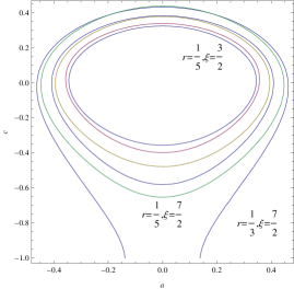
Figure 2: Curves for the ratio $\Delta m_{32}^{2}/\Delta m_{31}^{2}=30$ in the parameter space $(a,c)$.

Having checked that the parameters $a,c$ are in the perturbative range, while consistent with the mass data, we proceed to the mixing matrix. We can find easily numerical solutions for a wide range of the parameters consistent with the experimental data. In our approach, we have assumed a negligible mixing in the charged lepton sector therefore, the large mixing effects of the lepton mixing matrix $V=V_{\ell}^{\dagger}V_{\nu}$ relevant to experiment, are expected from the neutral sector.

Therefore, for our present purposes we assume almost diagonal $V_{\ell}$ and only consider the neutrino mixing matrix. Moreover, to simplify further the analysis in the present application, we will reduce the parameter space by imposing the condition $c+r=1$. This simplification is motivated by the most general structure of the the TB-mixing matrix in (1.5) where the relation $m_{12}=m_{13}$ holds. Of course in this way we restrict our investigations to a smaller portion of the full parameter space, but our purposes here is to only show that large mixing effects consistent with experiments are naturally accommodated in these models.

We use the ranges of the elements $V_{ij}$ as they are determined by the present-day experiments and vary $a,c$ to see if there are consistent values of the latter. We first observe that the elements $V_{23},V_{33}$ allow a wide range of values. Significant restrictions arise only from the elements $V_{11},V_{12},V_{13}$. In figure 3 we plot the bounds put by the experimental ranges [33]. In particular we plot the neutrino mixing entries for the following ranges

$$V_{11}=[0.795-0.846],V_{12}=[0.513-0.585],V_{13}=[]0.126-0.178],V_{22}=[0.416-0.730]$$

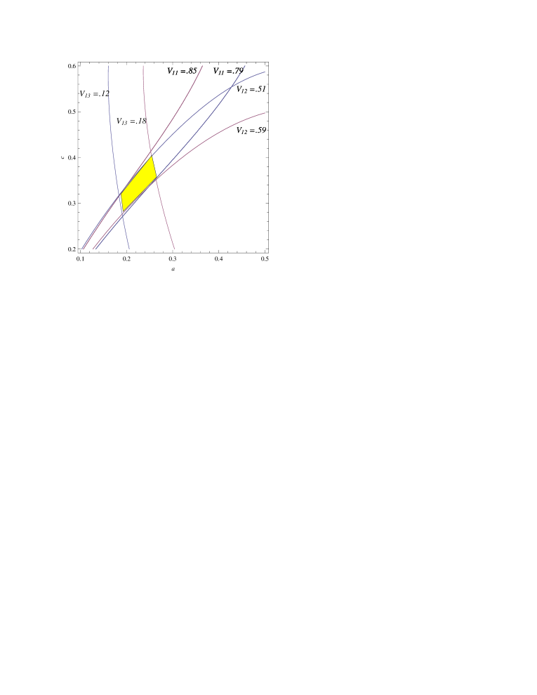
Figure 3: Bounds in the parameter space $(a,c)$ from the experimental range of neutrino mixing $V_{\nu}$ elements.

We notice that indeed, there exists an overlapping region where all the constraints imposed by the $V_{ij}$ ranges dictated by the neutrino experiments are satisfied. Furthermore, the $a,c$ parameters take values $<1$ in consistency with the requirements that the singlet vevs should be in the perturbative regime $\langle\theta_{ij}\rangle<M_{X}$. Note however, that in this restricted region the mass-square differences ratio comes out to be larger than the experimental value (4.23), but renormalization group effects are expected to change this in any case.

5 Conclusions

In this work we have investigated the neutrino properties in local F-theory GUT models which are realised on singular CY four-folds. We focused on the minimal unified symmetry $SU(5)_{GUT}$ embedded in the exceptional group $E_{8}$ in the elliptic fibration, and the properties emerging from its associated spectral cover ${\cal C}_{5}$ possessing an $SU(5)_{\perp}$ symmetry. To reproduce known neutrino properties such as large mixing which is nearly maximal among two generations, we consider the splitting ${\cal C}_{5}\to{\cal C}_{4}\times{\cal C}_{1}$ of spectral cover and study all possible monodromies ‘disguised’ as surrogate discrete symmetries in the low energy effective theory limit. We worked out constraints on the fermion mass structure with respect to the monodromies of the ${\cal C}_{4}$ part, and in particular to those associated to the permutation symmetries $S_{4},A_{4}$ as well as several of its subgroups. We paid particular attention to the leptonic sector and derived the charged lepton and neutrino mass textures for two models based on $A_{4}$ and ${Z}_{2}\times{Z}_{2}$ family symmetries. In the $A_{4}$ model right-handed neutrinos are not introduced and consequently the effective neutrino mass matrix is assumed to arise from a fifth order non-renormalisable operator. It is found that such a symmetry imposes significant restrictions on the F-theory models since there is only a limited number of matter curves to accommodate fermion families. Interestingly, however, the study of the leptonic sector shows that large mixing effects compatible with the recent neutrino data can be accommodated naturally. The second model we have examined is based on a ${Z}_{2}\times{Z}_{2}$ family symmetry. In this model the lepton sector includes also right handed neutrinos represented by appropriate massive KK states. This model also induces a large lepton mixing matrix in a natural way. Thus, we found that large lepton mixing effects are a generic property of these F-theory constructions. In particular, this property is linked directly to the neutral part of the lepton sector, while the charged lepton mixing matrix in both cases is found to be small.

Acknowledgements: This research has been co-financed by the European Union (European Social Fund - ESF) and Greek national funds through the Operational Program ”Education and Lifelong Learning” of the National Strategic Reference Framework (NSRF) - Research Funding Program: ”ARISTEIA”. Investing in the society of knowledge through the European Social Fund. This work was supported in part by the European Commission under the ERC Advanced Grant 226371 and the contract PITN-GA-2009- 237920. GKL would like to thank Theory Division, CERN for kind hospitality.

Appendix

We present here several computations and details with regard to the discriminant $\Delta(a_{i})$ of the fourth degree polynomial associated to ${\cal C}_{4}$-spectral cover. Since we express $\Delta(a_{i})$ as a polynomial with respect to one of its parameters $a_{i}$, we first start with some properties of the factorisation.

Appendix A The factorisation of the polynomial

We are interested in factorisations of the polynomial whose coefficients $c_{k}$ belong to a definite field ${\cal F}$. Consider the general fourth-degree one

$$P_{4}=c_{4}x^{4}+c_{3}x^{3}+c_{2}x^{2}+c_{1}x+c_{0}$$

with $c_{4}>0$. We wish to write the polynomial as a square

$$P_{4}=(b_{2}x^{2}+b_{1}x+b_{0})^{2}$$

This implies

$$b_{2}=\sqrt{c_{4}},\;b_{0}=\sqrt{c_{0}}$$

and various relations among the coefficients.

Since we assume $c_{k}\in{\cal F}$ and we also want $b_{k}\in{\cal F}$ we readily conclude that $\sqrt{c_{4}}$ and $\sqrt{c_{0}}$ must be in ${\cal F}$ too:

$$\sqrt{c_{4}},\sqrt{c_{0}}\in{\cal F}$$

Next, assume a fourth-degree polynomial of the particular form

$$P_{4}(x)=(x^{2}+2\kappa x+\lambda^{2})^{2}-\mu^{4}$$ (A.1)

This can split to two factors

$$P_{4}(x)=(x^{2}+2\kappa x+\lambda^{2}+\mu^{2})(x^{2}+2\kappa x+\lambda^{2}-\mu^{2})$$

while it is automatically a square when $\mu=0$.

Computing the discriminant we find

$$\Delta_{P_{4}}=256\mu^{8}\left(\left(\kappa^{2}-\lambda^{2}\right)^{2}-\mu^{4}\right)$$ (A.2)

Therefore, when the discriminant is zero the following possibilities emerge

$$\Delta_{P_{4}}=0\leftrightarrow\left\{\begin{array}[]{lcl}\mu=0&\Rightarrow&P_{4}=\delta^{2}\\ \mu^{2}=|\kappa^{2}-\lambda^{2}|&\Rightarrow&P_{4}=\delta_{1}\,\delta_{2}\end{array}\right.$$ (A.5)

with

$$\delta = (x^{2}+2\kappa x+\lambda^{2})$$ (A.6)

$$\delta_{1} = (x+\kappa)^{2}$$ (A.7)

$$\delta_{2} = x^{2}+2\kappa x+2\lambda^{2}-\kappa^{2}$$ (A.8)

Unless further relations are imposed among $\kappa,\lambda,\mu$, we observe that only one of the two zeros of the discriminant implies $P_{4}=\delta^{2}$, the other just giving a simple factorisation $P_{4}=\delta_{1}\delta_{2}$.

Appendix B The Discriminant

The starting point to achieve an $S_{4}$ discrete subgroup such as $A_{4}$ is to study the conditions on the factorisation of the discriminant and for $A_{4}$ is particular to write it as a square $\Delta=\delta^{2}$. In this appendix we will use the following $b_{1}=0$ condition

$$\left\{a_{4}\to-a_{0}a_{6},a_{5}\to a_{0}a_{7}\right\}$$

and substitute to the determinant $S_{d}$ in (3.8). Then $S_{d}$ takes the form

$$\begin{split}S_{d}=&a_{0}^{2}a_{7}\left(-27a_{0}^{3}a_{1}^{2}a_{6}^{4}+4a_{3}^{3}\left(4a_{1}a_{3}-a_{2}^{2}\right)a_{7}+a_{0}\left(a_{3}^{2}\left(a_{2}^{2}-4a_{1}a_{3}\right)a_{6}^{2}\right.\right.\\ &\left.\left.+2a_{2}a_{3}\left(40a_{1}a_{3}-9a_{2}^{2}\right)a_{7}a_{6}+\left(-27a_{2}^{4}+144a_{1}a_{3}a_{2}^{2}-128a_{1}^{2}a_{3}^{2}\right)a_{7}^{2}\right)\right.\\ &\left.+2a_{0}^{2}\left(a_{2}\left(2a_{2}^{2}-9a_{1}a_{3}\right)a_{6}^{3}-3a_{1}\left(a_{2}^{2}-24a_{1}a_{3}\right)a_{7}a_{6}^{2}+96a_{1}^{2}a_{2}a_{7}^{2}a_{6}+128a_{1}^{3}a_{7}^{3}\right)\right)\end{split}$$ (B.1)

Then, the discriminant is given by

$$\Delta=\frac{1}{a_{5}}S_{d}=\frac{1}{a_{0}a_{7}}S_{d}$$

We wish to investigate under what conditions this is separable with factors expressed in terms of coefficients $\in{\cal F}$. Noticing that $\Delta$ can be expressed as a polynomial of a given coefficient $P(a_{k})$, according to the discussion above we can factorise $P(a_{k})$ by imposing the condition that its own discriminant is zero. Expanding the discriminant as a polynomial of the various coefficients $a_{k}$ we obtain

$$\begin{split}f_{5}&=0\,{\bf a_{5}^{4}}+256a_{1}^{3}{\bf a_{5}^{3}}+\cdots\\ f_{4}&=-27a_{1}^{2}{\bf a_{4}^{4}}+\cdots\\ f_{3}&=16a_{1}a_{5}{\bf a_{3}^{4}}+\cdots\\ f_{2}&=-27a_{5}^{2}{\bf a_{2}^{4}}+\cdots\\ f_{1}&=0\,{\bf a_{1}^{4}}+256a_{5}^{3}{\bf a_{1}^{3}}+\cdots\end{split}$$ (B.2)

A few remarks are in order:

1. For real $a_{1},a_{5}$, the polynomials $f_{2},f_{4}$ have a negative coefficient, therefore cannot be positive definite.

2. $f_{5},f_{1}$ are cubic polynomials and and a necessary condition to be positive definite is sign$({a_{1}a_{5}})=(+)$.

3. The remaining possibility is $f_{3}$ is also positive definite for sign$({a_{1}a_{5}})=(+)$. We will choose to work out this case for the reasons discussed in the text.

4. This polynomial has the general form

   $$f_{3}=c_{4}a_{3}^{4}+c_{3}a_{3}^{3}+c_{2}a_{3}^{2}+c_{1}a_{3}+c_{0}$$

   ($c_{4}>0$) or written as a square:

   $$f_{3}=(b_{2}a_{2}^{2}+b_{1}a_{2}+b_{0})^{2}$$

   We have just seen that $b_{2}=\sqrt{c_{4}},\;b_{0}=\sqrt{c_{0}}$ and since we assume $c_{k}\in{\cal F}$ and we also want $b_{k}\in{\cal F}$ we readily conclude that $\sqrt{c_{4}}$ and $\sqrt{c_{0}}$ must be in ${\cal F}$ too:

   $$\sqrt{c_{4}},\sqrt{c_{0}}\in{\cal F}$$

   In our case, for $c_{4}$ we must have

   $$c_{4}\sim a_{1}a_{5}=a_{0}a_{1}a_{7}=e_{3}^{2},\;\;e_{3}\in{\cal F}$$

   while $c_{0}$ has a complicated form. Instead, we can extract some useful relations from the discriminant.

B.1 Analysis of $f_{3}$ case

Computing the discriminant of $f_{3}$ , we find that it is proportional to $\Delta_{f_{3}}\propto D_{a}^{2}D_{b}^{3}$ with

$$\begin{split}D_{a}&=a_{1}a_{4}^{2}-a_{2}^{2}a_{5}\\ D_{b}&=\left(27a_{1}^{2}a_{4}-a_{2}^{3}\right)a_{4}^{3}-6a_{1}a_{2}^{2}a_{5}a_{4}^{2}+4096a_{1}^{3}a_{5}^{3}+3a_{2}\left(9a_{2}^{3}-256a_{1}^{2}a_{4}\right)a_{5}^{2}\end{split}$$ (B.3)

Therefore, the discriminant is zero either when $D_{a}=0$ or if $D_{b}=0$.

We will see that, in accordance with what we have seen above, one condition, namely $D_{a}=0$, leads to a factorisation of the polynomial $f_{3}(a_{3})\to\Delta\,=\,\delta_{1}\delta_{2}$ while to succeed writing $f_{3}(a_{3})\to\Delta\,=\,\delta^{2}$ further conditions should be met. Next, we will see what conditions emerge from the second case.

B.1.1 $D_{a}=0$ case

We combine now the $a_{1}a_{5}=e_{3}^{2}$ condition with $D_{a}=0$:

$$a_{1}a_{4}^{2}=a_{2}^{2}a_{5}$$ (B.4)

From $a_{1}D_{a}=0$

$$(a_{1}a_{4})^{2}=a_{2}^{2}a_{1}a_{5}=(a_{2}e_{3})^{2}$$

thus $a_{1}a_{4}=\pm e_{3}a_{2}$. From $a_{5}D_{a}=0$ we also get $a_{2}a_{5}=\pm e_{3}a_{4}$. Therefore, summarising, we end up with the following set of relations

$$\begin{split}a_{1}a_{4}&=\pm e_{3}a_{2}\\ a_{2}a_{5}&=\pm e_{3}a_{4}\\ a_{1}a_{5}&=e_{3}^{2}\end{split}$$ (B.5)

To correlate the signs we multiply the second by $a_{1}$ and get $a_{2}a_{1}a_{5}=\xi\,e_{3}a_{1}a_{4}$ with $\xi=\pm 1$. We substitute $a_{1}a_{5}=e_{3}^{2}$ in the first term to obtain $e_{3}^{2}a_{5}=\xi\,e_{3}a_{1}a_{4}$ or $a_{2}e_{3}=\xi\,a_{1}a_{4}$.

The polynomial with respect to $a_{3}$ is

$$f_{3}=c_{4}a_{3}^{4}+c_{3}a_{3}^{3}+c_{2}a_{3}^{2}+c_{1}a_{3}^{1}+c_{0}$$

with coefficients

$$\begin{split}c_{4}&=16a_{1}a_{5}\\ c_{3}&=-4(a_{5}a_{2}^{2}+a_{1}a_{4}^{2})\\ c_{2}&=a_{2}^{2}a_{4}^{2}-80a_{2}a_{4}a_{1}a_{5}-128a_{1}^{2}a_{5}^{2}\\ c_{1}&=18a_{4}a_{5}a_{2}^{3}+144a_{1}a_{5}^{2}a_{2}^{2}+18a_{1}a_{4}^{3}a_{2}+144a_{1}^{2}a_{4}^{2}a_{5}\\ c_{0}&=-\left(4a_{2}^{3}+27a_{1}^{2}a_{4}\right)a_{4}^{3}-6a_{1}a_{2}^{2}a_{5}a_{4}^{2}+256a_{1}^{3}a_{5}^{3}-3a_{2}\left(9a_{2}^{3}+64a_{1}^{2}a_{4}\right)a_{5}^{2}\end{split}$$ (B.6)

Now we use the relations

$$a_{4}=\xi e_{3}a_{2},\;a_{1}a_{5}=e_{3}^{2}$$ (B.7)

whilst we introduce the redefinitions,

$$e_{3}a_{1}\to\beta_{2}^{2},\;a_{1}a_{3}\to x$$ (B.8)

so that the polynomial $f_{3}$ takes the form

$$16x^{4}-8a_{2}^{2}x^{3}+(a_{2}^{4}-80a_{2}^{2}\beta_{2}^{2}-128\beta_{2}^{4})x^{2}+36a_{2}^{2}\beta_{2}^{2}\left(a_{2}^{2}+8\beta_{2}^{2}\right)x+4\beta_{2}^{2}\left(\beta_{2}^{2}-a_{2}^{2}\right)\left(a_{2}^{2}+8\beta_{2}^{2}\right)^{2}$$

Clearly this cannot be automatically a square, however, it is easy to notice that this case corresponds to the second case of (A.5), i.e., when $\Delta_{f_{3}}=\delta_{1}\delta_{2}$. Indeed, after some algebra we find

$$\begin{split}f_{3}&=\left(a_{2}^{2}+8\beta_{2}^{2}-4x\right){}^{2}\left(\left(2\beta_{2}^{2}+x\right)^{2}-4a_{2}^{2}\beta_{2}^{2}\right)\end{split}$$ (B.9)

Now, we impose the relation

$$2x\to 2a_{1}a_{3}=a_{2}^{2}$$ (B.10)

Substitution of the above in (B.9) yields

$$\begin{split}f_{3}&=\left(a_{2}^{2}+8\beta_{2}^{2}-2a_{2}^{2}\right){}^{2}\left(\left(2\beta_{2}^{2}+a_{2}^{2}/2\right)^{2}-4a_{2}^{2}\beta_{2}^{2}\right)\\ &=\frac{1}{4}\left(\left(8\beta_{2}^{2}-a_{2}^{2}\right)\left(4\beta_{2}^{2}-a_{2}^{2}\right)\right)^{2}\\ &=\frac{1}{4}\left[a_{1}^{2}\left(8\,e_{3}-a_{3}\right)\left(4\,e_{3}-a_{3}\right)\right]^{2}\end{split}$$ (B.11)

where we have used consecutively the relations in (B.7) and (B.8). Hence, we have succeeded to write $f_{3}\to\Delta_{f_{3}}=\delta^{2}$ with

$$\delta=\frac{1}{2}\,a_{1}^{2}\left(8\,e_{3}-a_{3}\right)\left(4\,e_{3}-a_{3}\right)$$ (B.12)

If we combine the two relations (B.4) and (B.8) we find

$$\begin{split}a_{2}^{2}&=2\,a_{1}\,a_{3}\\ a_{4}^{2}&=2\,a_{3}\,a_{5}\end{split}$$ (B.13)

Using (B.13) we rewrite $\Delta=\delta^{2}$ only in terms of the initial coefficients $a_{k}$:

$$a_{3}^{6}\Delta\;=\;\left(a_{3}^{3}\delta\right)^{2}\;=\;\left[a_{2}a_{4}\left(a_{3}^{2}-2\,a_{2}a_{4}\right)\left(a_{3}^{2}-a_{2}a_{4}\right)\right]^{2}$$ (B.14)

In the subsequent analysis we examine the case $D_{b}=0$ which also leads to a simple condition among the coefficients $a_{k}$.

B.1.2 Factorisation of matter curves

One of the main goals is to use these relations to factorise appropriately the matter curves. For the case of the $\Sigma_{5}$ curve, we have seen that when the symmetry is $S_{4}$ it splits to two pieces $P_{5}=P_{5}^{a}P_{5}^{b}$. Further splitting can occur using the $D_{a}=0$ relation. For example, multiplying $a_{0}P_{5}^{a}$ we have

$$\begin{split}a_{0}P_{5}^{a}&=a_{0}(a_{2}^{2}a_{7}+a_{2}a_{3}a_{6}+a_{0}a_{1}a_{6}^{2})\\ &=a_{2}^{2}(a_{0}a_{7})+a_{2}a_{3}(a_{0}a_{6})+a_{1}(a_{0}a_{6})^{2}\\ &=a_{2}^{2}a_{5}-a_{2}a_{3}a_{4}+a_{1}a_{4}^{2}\\ &=a_{1}a_{4}^{2}-a_{2}a_{3}a_{4}+a_{1}a_{4}^{2}\\ &=a_{4}(2a_{1}a_{4}-a_{2}a_{3})\\ &=a_{0}a_{6}(2a_{0}a_{1}a_{6}-a_{2}a_{3})\end{split}$$ (B.15)

where we have used successively the $b_{1}=0$ and $D_{a}=0$ conditions. Eliminating $a_{0}$ from the first and last lines of the above, we get

$$P_{5}^{a}=a_{6}(2a_{0}a_{1}a_{6}-a_{2}a_{3})$$

Therefore the fiveplets’ equation separates now to three distinct curves

$$P_{5}=a_{6}(2a_{0}a_{1}a_{6}-a_{2}a_{3})\left(a_{3}a_{6}^{2}+\left(a_{2}a_{6}+a_{1}a_{7}\right)a_{7}\right)$$

B.1.3 The $D_{b}=0$ case

The vanishing of the discriminant $\Delta_{f_{3}}$ can happen also when the second factor in (B.3) is set to zero, i.e. $D_{b}=0$, which leads to analogous relations among $a_{k}$. Indeed, it can be readily checked that this factor can be brought to the form

$$\begin{split}D_{b}&=(16)^{3}(a_{1}a_{5})^{3}\\ &-3\cdot(16)^{2}(a_{1}a_{5})^{2}(a_{2}a_{4})\\ &+27(a_{2}^{4}a_{5}^{2}+a_{4}^{4}a_{1}^{2})\\ &-6(a_{1}a_{5})(a_{2}a_{4})^{2}\\ &-(a_{2}a_{4})^{3}\end{split}$$ (B.16)

Observing the third term, we can easily recognise that conditions (B.5) transform this term to

$$(a_{2}^{4}a_{5}^{2}+a_{4}^{4}a_{1}^{2})=2(e_{3}a_{2}a_{4})^{2}\equiv 2(a_{1}a_{5})(a_{2}a_{4})^{2}$$

Substituting to (B.16) we get

$$D_{b}=(16a_{1}a_{5}-a_{2}a_{4})^{3}$$ (B.17)

This could be solved for a particular relation among the coefficients, namely $a_{2}a_{4}=16a_{1}a_{5}\sim 16\,e_{3}^{2}$ however, we implicitly used the condition $D_{a}=0$ which overconstrains the system of the coefficients.

In fact, the requirement to have the condition $\Delta=\delta^{2}$ is more involved and the general solution should be found without the implicit use of the result of the first case.

Indeed, we can solve the $D_{b}=0$ directly. Introducing $x=a_{1}a_{5},y=a_{2}a_{4}$, we get

$$\begin{split}27(a_{2}^{4}a_{5}^{2}+a_{4}^{4}a_{1}^{2})&=y^{3}+6xy^{2}+3(16x)^{2}y-(16x)^{3}\\ &=(y-16x)^{3}+54xy^{2}\end{split}$$ (B.18)

Therefore the relation among the coefficients implying $\Delta=\delta^{2}$ is

$$a_{2}^{4}a_{5}^{2}+a_{4}^{4}a_{1}^{2} = \left(\frac{16a_{1}a_{5}-a_{2}a_{4}}{3}\right)^{3}+2(a_{1}a_{5})(a_{2}a_{4})^{2}$$ (B.19)

Rearranging the term $2(a_{1}a_{5})(a_{2}a_{4})^{2}=2(a_{1}a_{4}^{2})(a_{5}^{2}a_{2})$ and moving it to the left-hand side of the latter equation we notice that it can be further simplified and written as an “elliptic curve” formula $Y^{2}=X^{3}$:

$$(a_{2}^{2}a_{5}-a_{4}^{2}a_{1})^{2} = \left(\frac{16a_{1}a_{5}-a_{2}a_{4}}{3}\right)^{3}$$ (B.20)

Plugging in the condition $b_{1}=0$ yields

$$(a_{2}^{2}a_{7}-a_{0}a_{1}a_{6}^{2})^{2} = a_{0}\left(\frac{16a_{1}a_{7}+a_{2}a_{6}}{3}\right)^{3}$$ (B.21)

References

• [1] C. Beasley, J. J. Heckman and C. Vafa, “GUTs and Exceptional Branes in F-theory - I,” JHEP 0901 (2009) 058 [arXiv:0802.3391 [hep-th]].
• [2] R. Donagi and M. Wijnholt, “Breaking GUT Groups in F-Theory,” Adv. Theor. Math. Phys.  15 (2011) 1523 [arXiv:0808.2223 [hep-th]].
• [3] C. Beasley, J. J. Heckman and C. Vafa, “GUTs and Exceptional Branes in F-theory - II: Experimental Predictions,” JHEP 0901 (2009) 059 [arXiv:0806.0102 [hep-th]].
• [4] R. Donagi and M. Wijnholt, “Model Building with F-Theory,” Adv. Theor. Math. Phys.  15 (2011) 1237 [arXiv:0802.2969 [hep-th]].
• [5] R. Donagi and M. Wijnholt, “Higgs Bundles and UV Completion in F-Theory,” arXiv:0904.1218 [hep-th].
• [6] J. J. Heckman, “Particle Physics Implications of F-theory,” Ann. Rev. Nucl. Part. Sci.  60 (2010) 237 [arXiv:1001.0577 [hep-th]].
• [7] T. Weigand, “Lectures on F-theory compactifications and model building,” Class. Quant. Grav.  27 (2010) 214004 [arXiv:1009.3497 [hep-th]].
• [8] G. K. Leontaris, “Aspects of F-Theory GUTs,” PoS CORFU 2011 (2011) 095 [arXiv:1203.6277 [hep-th]].
• [9] A. Maharana and E. Palti, “Models of Particle Physics from Type IIB String Theory and F-theory: A Review,” Int. J. Mod. Phys. A 28 (2013) 1330005 [arXiv:1212.0555 [hep-th]].
• [10] S. Cecotti, M. C. N. Cheng, J. J. Heckman and C. Vafa, “Yukawa Couplings in F-theory and Non-Commutative Geometry,” arXiv:0910.0477 [hep-th].
• [11] A. Font and L. E. Ibanez, “Matter wave functions and Yukawa couplings in F-theory Grand Unification,” JHEP 0909 (2009) 036 [arXiv:0907.4895 [hep-th]].
• [12] A. Font, L. E. Ibanez, F. Marchesano and D. Regalado, “Non-perturbative effects and Yukawa hierarchies in F-theory SU(5) Unification,” JHEP 1303 (2013) 140 [arXiv:1211.6529 [hep-th]].
• [13] E. Dudas and E. Palti, “Froggatt-Nielsen models from E(8) in F-theory GUTs,” JHEP 1001 (2010) 127 [arXiv:0912.0853 [hep-th]].
• [14] S. F. King, G. K. Leontaris and G. G. Ross, “Family symmetries in F-theory GUTs,” Nucl. Phys. B 838 (2010) 119 [arXiv:1005.1025 [hep-ph]].
• [15] E. Dudas and E. Palti, “On hypercharge flux and exotics in F-theory GUTs,” JHEP 1009 (2010) 013 [arXiv:1007.1297 [hep-ph]].
• [16] G. K. Leontaris and G. G. Ross, “Yukawa couplings and fermion mass structure in F-theory GUTs,” JHEP 1102 (2011) 108 [arXiv:1009.6000 [hep-th]].
• [17] P. G. Camara, E. Dudas and E. Palti, “Massive wavefunctions, proton decay and FCNCs in local F-theory GUTs,” JHEP 1112 (2011) 112 [arXiv:1110.2206 [hep-th]].
• [18] J. C. Callaghan, S. F. King, G. K. Leontaris and G. G. Ross, “Towards a Realistic F-theory GUT,” JHEP 1204 (2012) 094 [arXiv:1109.1399 [hep-ph]].
J. C. Callaghan and S. F. King, “E6 Models from F-theory,” JHEP 1304, 034 (2013) [arXiv:1210.6913 [hep-ph]].
• [19] I. Antoniadis and G. K. Leontaris, “Building SO(10) models from F-theory,” JHEP 1208 (2012) 001 [arXiv:1205.6930 [hep-th]].
• [20] J. Pawelczyk, “A F-GUT inspired model of Yukawa couplings with matter-messenger unification,” arXiv:1305.5162 [hep-ph].
• [21] I. de Medeiros Varzielas, S. F. King and G. G. Ross, “Neutrino tri-bi-maximal mixing from a non-Abelian discrete family symmetry,” Phys. Lett. B 648 (2007) 201 [hep-ph/0607045].
G. Altarelli and F. Feruglio, “Discrete Flavor Symmetries and Models of Neutrino Mixing,” Rev. Mod. Phys.  82 (2010) 2701 [arXiv:1002.0211 [hep-ph]].
H. Ishimori, T. Kobayashi, H. Ohki, Y. Shimizu, H. Okada and M. Tanimoto, “Non-Abelian Discrete Symmetries in Particle Physics,” Prog. Theor. Phys. Suppl.  183 (2010) 1 [arXiv:1003.3552 [hep-th]].
S. F. King and C. Luhn, “Neutrino Mass and Mixing with Discrete Symmetry,” Rept. Prog. Phys.  76 (2013) 056201 [arXiv:1301.1340 [hep-ph]].
R. N. Mohapatra, S. Antusch, K. S. Babu, G. Barenboim, M. -C. Chen, A. de Gouvea, P. de Holanda and B. Dutta et al., “Theory of neutrinos: A White paper,” Rept. Prog. Phys.  70 (2007) 1757 [hep-ph/0510213].
• [22] L. E. Ibanez and G. G. Ross, “Discrete gauge symmetry anomalies,” Phys. Lett. B 260 (1991) 291.
P. Anastasopoulos, M. Cvetic, R. Richter and P. K. S. Vaudrevange, “String Constraints on Discrete Symmetries in MSSM Type II Quivers,” JHEP 1303 (2013) 011 [arXiv:1211.1017 [hep-th]].
H. M. Lee, S. Raby, M. Ratz, G. G. Ross, R. Schieren, K. Schmidt-Hoberg and P. K. S. Vaudrevange, “A unique $Z_{4}^{R}$ symmetry for the MSSM,” Phys. Lett. B 694 (2011) 491 [arXiv:1009.0905 [hep-ph]].
L. E. Ibanez, A. N. Schellekens and A. M. Uranga, “Discrete Gauge Symmetries in Discrete MSSM-like Orientifolds,” Nucl. Phys. B 865 (2012) 509 [arXiv:1205.5364 [hep-th]].
• [23] M. Berasaluce-Gonzalez, P. G. Camara, F. Marchesano, D. Regalado and A. M. Uranga, “Non-Abelian discrete gauge symmetries in 4d string models,” JHEP 1209 (2012) 059 [arXiv:1206.2383 [hep-th]].
• [24] J. Marsano, N. Saulina and S. Schafer-Nameki, “Monodromies, Fluxes, and Compact Three-Generation F-theory GUTs,” JHEP 0908 (2009) 046 [arXiv:0906.4672 [hep-th]].
• [25] J. Tate, “Algorithm for Determining the Type of a Singular Fiber in an Elliptic Pencil,” in Modular Functions of One Variable IV, Lecture Notes in Math. vol. 476, Springer-Verlag, Berlin (1975).
• [26] K. -S. Choi, “SU(3) x SU(2) x U(1) Vacua in F-Theory,” Nucl. Phys. B 842, 1 (2011) [arXiv:1007.3843 [hep-th]].
• [27] H. Hayashi, T. Kawano, Y. Tsuchiya and T. Watari, “Flavor Structure in F-theory Compactifications,” JHEP 1008 (2010) 036 [arXiv:0910.2762 [hep-th]].
• [28] J. Marsano, H. Clemens, T. Pantev, S. Raby and H. -H. Tseng, “A Global SU(5) F-theory model with Wilson line breaking,” JHEP 1301 (2013) 150 [arXiv:1206.6132 [hep-th]].
• [29] Michael Artin, ”Algebra”, Prentice-Hall Inc. 1991.
Patrick Morandi, ”Field and Galois Theory”, Springer, 1996.
• [30] C. Luhn, S. Nasri and P. Ramond, “Tri-bimaximal neutrino mixing and the family symmetry semidirect product of Z(7) and Z(3),” Phys. Lett. B 652 (2007) 27 [arXiv:0706.2341 [hep-ph]].
• [31] I. Antoniadis, E. Kiritsis, J. Rizos and T. N. Tomaras, “D-branes and the standard model,” Nucl. Phys. B 660 (2003) 81 [hep-th/0210263].
• [32] V. Bouchard, J. J. Heckman, J. Seo and C. Vafa, “F-theory and Neutrinos: Kaluza-Klein Dilution of Flavor Hierarchy,” JHEP 1001 (2010) 061 [arXiv:0904.1419 [hep-ph]].
• [33] M. C. Gonzalez-Garcia, M. Maltoni, J. Salvado and T. Schwetz, “Global fit to three neutrino mixing: critical look at present precision,” JHEP 1212 (2012) 123 [arXiv:1209.3023 [hep-ph]].