Simulating spin-$\mathbf{\frac{3}{2}}$ particles at colliders

Abstract

Support for interactions of spin-$\frac{3}{2}$ particles is implemented in the FeynRules and ALOHA packages and tested with the MadGraph 5 and CalcHEP event generators in the context of three phenomenological applications. In the first, we implement a spin-$\frac{3}{2}$ Majorana gravitino field, as in local supersymmetric models, and study gravitino and gluino pair-production. In the second, a spin-$\frac{3}{2}$ Dirac top-quark excitation, inspired from compositness models, is implemented. We then investigate both top-quark excitation and top-quark pair-production. In the third, a general effective operator for a spin-$\frac{3}{2}$ Dirac quark excitation is implemented, followed by a calculation of the angular distribution of the $s$-channel production mechanism.

CERN-PH-TH/2013-187, IPPP/13/56, DCPT/13/172,
MCNET-13-09, PITT-PACC-1307, KIAS-P13044,
TUM-HEP 900/13

1 Introduction

The recent discovery of the Higgs boson Aad:2012gk ; Chatrchyan:2012gu has greatly reinforced our expectation to find physics beyond the Standard Model (BSM) at the Large Hadron Collider (LHC). For the first time, we have discovered a particle in Nature which is intrinsically unstable with respect to quantum corrections and either requires unnaturally extreme fine-tuning or stabilization from a new sector of physics which will emerge at scales we will soon probe. Although we do not yet know which BSM theory will be the correct description of Nature, our current models often predict the presence of a spin-$\frac{3}{2}$ particle. For example, in models of supergravity Deser:1976eh ; Freedman:1976xh ; Freedman:1976py ; Ferrara:1976um ; Cremmer:1978hn ; Cremmer:1978iv ; Cremmer:1982en ; Cremmer:1982wb ; Witten:1982hu , the graviton is accompanied by a spin-$\frac{3}{2}$ gravitino superpartner. As another example, in models of compositeness, the top-quark has an associated spin-$\frac{3}{2}$ resonance Burges:1983zg ; Kuhn:1984rj ; Kuhn:1985mi ; Moussallam:1989nm ; Almeida:1995yp ; Dicus:1998yc ; Walsh:1999pb ; Cakir:2007wn ; Stirling:2011ya ; Dicus:2012uh ; Hassanain:2009at . On different footings, if a spin-$\frac{3}{2}$ particle were discovered at the LHC, until the full picture was complete, an effective operator approach would be appropriate for determining its properties. Because there are many models that Nature could choose for the description of a spin-$\frac{3}{2}$ particle, it is essential that we simulate and analyze the signatures of these particles from as wide a class of models as possible, in preparation for the day we find it at an experiment.

There is an assortment of well-established Monte-Carlo packages used for simulating the collisions of high energy physics, each with its own strengths. Among these are CalcHEP Pukhov:1999gg ; Boos:2004kh ; Pukhov:2004ca ; Belyaev:2012qa , MadGraph Stelzer:1994ta ; Maltoni:2002qb ; Alwall:2007st ; Alwall:2008pm ; Alwall:2011uj , Sherpa Gleisberg:2003xi ; Gleisberg:2008ta , and Whizard Moretti:2001zz ; Kilian:2007gr at parton level which are often followed by Pythia Sjostrand:2006za ; Sjostrand:2007gs , Sherpa, or Herwig Corcella:2000bw ; Bahr:2008pv for radiation and hadronization. Historically, these packages only supported the Standard Model (SM) and a very small subset of the models BSM. Until recently, spin-$\frac{3}{2}$ particles were not supported at all Belyaev:2012qa ; Kilian:2001qz ; Hagiwara:2010pi . The difficulty was that each model had to be implemented directly into the code of the respective Monte-Carlo packages. This process required: first, an intimate knowledge of the Monte-Carlo package code; second, the hand-coding of thousands of lines of code for the Feynman rules and the parameter’s dependence; and third, a long and tedious process of debugging. Fortunately, the status of implementing new models into these simulation packages has recently and dramatically improved. The first of these improvements is that the parton-level matrix element generators have begun to establish more general model input formats that require less intimate knowledge of their internal code. The second improvement is the presence of packages that allow the user to enter the Lagrangian of their model rather than the individual vertices. These packages then calculate the Feynman rules from the Lagrangian and export the model to the supported Monte-Carlo package of choice. The first of these packages was LanHEP Semenov:1996es ; Semenov:1998eb ; Semenov:2002jw ; Semenov:2008jy ; Semenov:2010qt followed more recently by FeynRules Christensen:2008py ; Christensen:2009jx ; Christensen:2010wz ; Duhr:2011se ; Fuks:2012im ; Alloul:2013fw and SARAH Staub:2008uz ; Staub:2012pb .

Although the status for implementing new models into Monte-Carlo packages has greatly improved, the situation for spin-$\frac{3}{2}$ has still been lacking. The purpose of this paper is to report the implementation of support for spin-$\frac{3}{2}$ particles in FeynRules, in its CalcHEP export interface, in its Universal FeynRules Output (UFO) export interface, in the UFO format Degrande:2011ua , in the Automatic Libraries Of Helicity Amplitude (ALOHA) package deAquino:2011ub and in MadGraph 5. We further use this chain of packages to implement the gravitino of supergravity together with its interactions and a model inspired by quark and lepton compositeness involving a spin-$\frac{3}{2}$ quark excitation. These implementations are then employed for reproducing several physics results of earlier studies.

This paper is organized as follows: Section 2 gives a brief introduction to spin-$\frac{3}{2}$ fields. Section 3 describes the implementation of spin-$\frac{3}{2}$ fields in FeynRules, UFO, ALOHA, MadGraph 5 and CalcHEP. Section 4 presents the phenomenological applications of these implementations for their validation. Section 5 summarizes our results. We collect our conventions on Pauli and Dirac matrices, epsilon tensors, etc., in Appendix A and include a review of spin, together with a detailed discussion of field polarization vectors and propagators, in Appendix B. Helicity amplitudes associated with gravitino pair-production, relevant for the discussion of Section 4.1.1, are given in Appendix C.

2 Spin-$\mathbf{\frac{3}{2}}$ fermion fields

The first relativistic description of spin-$\frac{3}{2}$ fermions was carried out by Rarita and Schwinger in 1941 Rarita:1941mf . This was achieved by introducing a generalized version of the Dirac equation, in which the spin-$\frac{3}{2}$ particles were described by a Dirac spinor with a Lorentz index, the so-called Rarita-Schwinger field. In modern notation, the free classical equation of motion for this field reads

$$(\epsilon^{\mu\nu\rho\sigma}\gamma_{5}\gamma_{\rho}\partial_{\sigma}+2iM\gamma^{\mu\nu})\Psi_{\nu}=0\;,$$ (1)

where $M$ is the mass of the spin-$\frac{3}{2}$ fermion described by $\Psi_{\nu}$, and the Lorentz generators in the (four-component) spinorial representation $\gamma^{\mu\nu}$ have been defined in Appendix A. In the language of group theory, the Rarita-Schwinger field belongs to the direct product of two representations of the Lorentz group: the vector representation $(\frac{1}{2},\frac{1}{2})$, which describes objects with one Lorentz index, and the Dirac representation $(\frac{1}{2},0)\oplus(0,\frac{1}{2})$, which describes a Dirac pair of spin-$\frac{1}{2}$ fermions. Altogether, this direct product contains one Dirac pair of spin-$\frac{3}{2}$ fermions and two Dirac pairs of spin-$\frac{1}{2}$ fermions,

$$\left(\frac{1}{2},\frac{1}{2}\right)\otimes\left[\left(\frac{1}{2},0\right)\oplus\left(0,\frac{1}{2}\right)\right]=\hskip 108.405pt$$ (2)

$$\hskip 72.26999pt\left(\frac{1}{2},1\right)\oplus\left(\frac{1}{2},0\right)\oplus\left(1,\frac{1}{2}\right)\oplus\left(0,\frac{1}{2}\right)\ .$$

We observe that there is an ordinary Dirac spinor $(\frac{1}{2},0)\oplus(0,\frac{1}{2})$ in this direct product. This piece can be identified with $\gamma^{\nu}\Psi_{\nu}$, which transforms as a Dirac spinor, and can thus be removed by requiring that $\gamma^{\nu}\Psi_{\nu}=0$. Furthermore, the $(\frac{1}{2},1)\oplus(1,\frac{1}{2})$ piece is reducible under the little group and contains a pair of spin-$\frac{1}{2}$ fermions in addition to the pair of spin-$\frac{3}{2}$ fermions that we are after. This last pair of spin-$\frac{1}{2}$ fermions can be identified with $\partial^{\nu}\Psi_{\nu}$, which again transforms as a Dirac spinor. This piece can be removed by requiring $\partial^{\nu}\Psi_{\nu}=0$. Both of these equations, as well as the Dirac equation, are a result of the free classical equation of motion. That is, Eq. (1) implies

$$\gamma^{\nu}\Psi_{\nu}=0\ ,\hskip 20.0pt\partial^{\nu}\Psi_{\nu}=0\ ,\hskip 20.0pt(-i\not{\partial}+M)\Psi_{\nu}=0\ .$$ (3)

Consequently, on-shell, the free classical equations of motion remove the spin-$\frac{1}{2}$ fermions so that only the spin-$\frac{3}{2}$ fermions are left. However, since classical equations of motion, as well as the resulting Eq. (3), only apply on-shell, the two pairs of spin-$\frac{1}{2}$ fermions can be present in the case of off-shell spin-$\frac{3}{2}$ fields.

An important example of a (Majorana) spin-$\frac{3}{2}$ field is in supergravity theories where supersymmetry requires the spin-$2$ graviton to have a superpartner, the gravitino, with spin $\frac{3}{2}$. In such models, it is often more convenient to work in a two-component notation instead of the four-component notation introduced by Rarita and Schwinger. In this case, the free field Lagrangian reads

$$\begin{split}{\cal L}=&\frac{1}{2}\epsilon^{\mu\nu\rho\sigma}(\psi_{\mu}\sigma_{\rho}\partial_{\sigma}{\bar{\psi}}_{\nu}+\partial_{\sigma}\psi_{\nu}\sigma_{\rho}{\bar{\psi}}_{\mu})\\ &+iM(\psi_{\mu}\sigma^{\mu\nu}\psi_{\nu}+\bar{\psi}_{\mu}\bar{\sigma}^{\mu\nu}\bar{\psi}_{\nu})\ ,\end{split}$$ (4)

where, now, $\psi_{\nu}$ ($\bar{\psi}_{\nu}$) represents the left-chiral (right-chiral) two-component spin-$\frac{3}{2}$ field. We recall that our conventions of the generators of the Lorentz algebra in the (two-component) spinorial representation are summarized in Appendix A. This Lagrangian leads to the two-component form of Eq. (3), after replacing the Dirac matrices by the Pauli matrices and the Dirac equation by the Weyl equation.

3 Spin-$\mathbf{\frac{3}{2}}$ implementation

3.1 FeynRules

FeynRules Christensen:2008py ; Christensen:2009jx ; Christensen:2010wz ; Duhr:2011se ; Fuks:2012im ; Alloul:2013fw is a Mathematica package that allows the user to compute Feynman rules for a model based on quantum field theory directly from the associated Lagrangian. It can be used for any model that satisfies locality as well as Lorentz and gauge invariance. More precisely, a necessary condition for FeynRules to work correctly is that all indices appearing in the Lagrangian are contracted. Moreover, no assumption is made on the dimensionality of the operators that appear inside the Lagrangian. This feature is particularly useful in the present case, as Lagrangians for spin-$\frac{3}{2}$ particles necessarily involve operators of dimension greater than four.

The output of FeynRules is generic enough to be exported into any other model format. Translation interfaces hence exist to convert the Feynman rules computed by FeynRules into a format readable by various Feynman diagram generators. Currently such translation interfaces have been developed for CalcHEP and CompHEP, FeynArts and FormCalc Hahn:1998yk ; Hahn:2000kx ; Hahn:2009bf ; Agrawal:2011tm , MadGraph 4, Sherpa as well as Whizard and O’Mega. In addition, the user has the possibility to output the Feynman rules in the so-called Universal FeynRules Output (UFO), a format for the implementation of new physics models into Feynman diagram generators that is not tied to any specific matrix element generator Degrande:2011ua .

In the rest of this section, we describe how particles of spin-$\frac{3}{2}$ can be implemented into FeynRules both in non-supersymmetric theories as well as in supersymmetric theories. In the following, we also detail the extension of the UFO (Section 3.2) and CalcHEP (Section 3.5) interfaces, respectively.

The implementation of spin-$\frac{3}{2}$ particles into FeynRules models follows the same logic as the implementation of all other particles. We therefore refer to the FeynRules manual Christensen:2008py for more details on the declaration of particle classes. One important difference with the manual is that it is now possible to implement both two- and four-component fermions Duhr:2011se . Four-component spin-$\frac{3}{2}$ fields correspond to the newly introduced particle class R, while two-component fields are implemented by declaring instances of the class RW. All the attributes common to the other particle classes are available for spin-$\frac{3}{2}$ fields, together with the option Chirality for two-component fields so that one can define both left and right-handed two-component spin-$\frac{3}{2}$ fields. Furthermore, each spin-$\frac{3}{2}$ field always carries by default an index of type Spin (respectively Spin1 and Spin2 for left-handed and right-handed two-component fields) as well as an index of type Lorentz. We stress that, when writing down a Lagrangian involving spin-$\frac{3}{2}$ fields, it is mandatory for the Spin and Lorentz indices to be the first two indices (in this order) carried by the spin-$\frac{3}{2}$ fields.

In supersymmetric theories, spontaneous supersymmetry breaking predicts the existence of a massless fermion, dubbed the goldstino. The way this field interacts with the rest of the particle spectrum can be derived from the conservation of the supercurrent. The latter is defined by the variation of the model Lagrangian ${\cal L}$ under a supersymmetry transformation with a (Majorana fermionic) parameter $(\varepsilon,{\bar{\varepsilon}})$,

$$\delta_{\varepsilon}{\cal L}=\partial_{\mu}K^{\mu}=\partial_{\mu}\bigg{[}{\partial{\cal L}\over\partial\big{(}\partial_{\mu}X\big{)}}\delta_{\varepsilon}X\bigg{]}\ .$$ (5)

We have used Euler-Lagrange equations to simplify the right-hand side of this equation, and a sum over all fields $X$ of the theory is implicit. Consequently, the (Majorana fermionic) supercurrent $(J^{\mu},{\bar{J}}^{\mu})$ is defined by

$$\varepsilon\!\cdot\!J^{\mu}+{\bar{\varepsilon}}\!\cdot\!{\bar{J}}^{\mu}={\partial{\cal L}\over\partial\big{(}\partial_{\mu}X\big{)}}\delta_{\varepsilon}X-K^{\mu}\ .$$ (6)

This is a conserved quantity since $\partial_{\mu}J^{\mu}=0$ and $\partial_{\mu}{\bar{J}}^{\mu}=0$. Following standard superspace techniques, $J^{\mu}$ can be computed as Wess:1978ns ; Iliopoulos:1974zv ; FuksRausch

$$\begin{split}J^{\mu}_{\alpha}=&\ \sqrt{2}D_{\nu}\phi^{\dagger}_{i}\big{(}\sigma^{\nu}{\bar{\sigma}}^{\mu}\psi^{i}\big{)}_{\alpha}+\sqrt{2}i\big{(}\sigma^{\mu}{\bar{\psi}}_{i}\big{)}_{\alpha}W^{\star i}\\ &\ +g\phi^{\dagger}T_{a}\phi\big{(}\sigma^{\mu}{\bar{\lambda}}^{a}\big{)}_{\alpha}-\frac{i}{2}\big{(}\sigma^{\rho}{\bar{\sigma}}^{\nu}\sigma^{\mu}{\bar{\lambda}}_{a}\big{)}_{\alpha}v^{a}_{\nu\rho}\ ,\end{split}$$ (7)

where sums over the model gaugino fields $\lambda$, two-component fermions $\psi$, scalar fields $\phi$ and vector bosons $v_{\mu}$ (the associated field strength tensors being denoted by $v_{\mu\nu}$) are implicitly accounted for. Moreover, we generically denote by $D_{\mu}$ gauge covariant derivatives, by $T^{a}$ and $g$ representation matrices and the coupling constant of the gauge group and by $W^{\star i}$ the derivatives of the hermitian conjugate superpotential $W^{\star i}\equiv\partial W^{\star}(\phi^{\dagger})/\partial\phi^{\dagger}_{i}$.

The supercurrent can be calculated in FeynRules by issuing, in a Mathematica session,

  SuperCurrent[lv,lc,lw,sp,mu]

where the variables lv, lc and lw are connected to the different pieces of the supersymmetric Lagrangian ${\cal L}_{v}$, ${\cal L}_{c}$ and ${\cal L}_{w}$ defined below, and sp and mu are spin and Lorentz indices, respectively. The three Lagrangians above must be given as full series expansions in terms of the Grassmann variables and read

$$\begin{split}{\cal L}_{v}=&\ \frac{1}{16g^{2}}\Big{[}W^{a\alpha}W_{a\alpha}+\bar{W}^{a}_{\dot{\alpha}}\bar{W}_{a}^{\dot{\alpha}}\Big{]}\ ,\\ {\cal L}_{c}=&\ \Phi^{\dagger}e^{-2gV}\Phi\ ,\\ {\cal L}_{w}=&\ W(\Phi)\ ,\end{split}$$ (8)

where sums over the whole chiral ($\Phi$) and vector ($V$) superfield content of the model are again understood. In these expressions, we have also introduced the superpotential $W(\Phi)$ and the superfield strength tensors $W_{\alpha}$ and $\bar{W}_{\dot{\alpha}}$. These three superfields can be automatically obtained in FeynRules by issuing

 lc = GrassmannExpand[ CSFKineticTerms[] ];
 lv = GrassmannExpand[ VSFKineticTerms[] ];
 lw = GrassmannExpand[ SPot+HC[SPot] ];

where the superpotential SPot is the only quantity to be provided by the user, in addition to all the model (super)field declarations. We refer to Ref. Duhr:2011se for more information.

Once extracted, the supercurrent can be further employed in the construction of effective Lagrangians for the goldstino and gravitino fields Fayet:1977vd ; Fayet:1979yb . In this context, one or several of the auxiliary fields of the supersymmetric model under consideration acquire vacuum expectation values. Supercurrent conservation is then understood as the equations of motion for the goldstino field. More explicitly, we take the example of a chiral supermultiplet $(\phi_{1},\psi_{1},F_{1})$ whose auxiliary field $F_{1}$ gets a vacuum expectation value $v_{1}/\sqrt{2}$. Supercurrent conservation then leads to

$$0=\partial_{\mu}J^{\mu}=iv_{1}(\sigma^{\mu}\partial_{\mu}\bar{\psi}_{1})_{\alpha}+\partial_{\mu}\tilde{J}^{\mu}_{\alpha}\ ,$$ (9)

after having shifted the field $F_{1}$ by its vacuum expectation value, the quantity $\tilde{J}$ containing all the other contributions to the supercurrent. Considering Eq. (9) as the equations of motion for the goldstino field identified here as $\psi_{1}$, one deduces the corresponding Lagrangian

$$\begin{split}{\cal L}_{\psi_{1}}=&\ \frac{i}{2}\Big{(}\psi_{1}\sigma^{\mu}\partial_{\mu}\bar{\psi}_{1}-\partial_{\mu}\psi_{1}\sigma^{\mu}\bar{\psi}_{1}\Big{)}\\ &\ +\frac{1}{2v_{1}}\Big{[}\psi_{1}\!\cdot\!\partial_{\mu}\tilde{J}^{\mu}+{\bar{\psi}}_{1}\!\cdot\!\partial_{\mu}\bar{\tilde{J}}^{\mu}\Big{]}\ .\end{split}$$ (10)

Once the goldstino has been eaten by the gravitino, the latter becomes massive and the Lagrangian can be rewritten in terms of the (two-component) spin-$\frac{3}{2}$ gravitino field $\psi_{G}$,

$$\begin{split}{\cal L}_{G}=&\ \frac{1}{2}\epsilon^{\mu\nu\rho\sigma}(\psi_{G\mu}\sigma_{\rho}\partial_{\sigma}{\bar{\psi}}_{G\nu}+\partial_{\sigma}\psi_{G\nu}\sigma_{\rho}{\bar{\psi}}_{G\mu})\\ &\ +{\cal N}\Big{[}\psi_{G\mu}\!\cdot\!J^{\mu}+{\bar{\psi}}_{G\mu}\!\cdot\!\bar{J}^{\mu}\Big{]}\ .\end{split}$$ (11)

where we have replaced the vacuum expectation value $v_{1}$ by the generic normalization constant ${\cal N}$. In general, the latter is expressed in terms of the supersymmetry-breaking scale and the gravitino mass. Both Lagrangians derived above can subsequently be implemented in FeynRules by making use of standard techniques.

3.2 UFO

The UFO format Degrande:2011ua is, by construction, completely agnostic of the model and the associated interactions. In particular, the format does not make any a priori assumptions about the color and/or Lorentz structures that appear inside the vertices. Therefore, higher-dimensional operators can be implemented in the same way as renormalizable operators.

On the other hand, the UFO format was implicitly assuming a particular convention for propagators. As explained in Appendix B.3, the propagator for spin-$\frac{3}{2}$ is not unique and more than one expression are commonly used in the literature. The same is true for the massless propagator which depends on the gauge fixing term VanNieuwenhuizen:1981ae . We therefore extend the UFO format in order to support model specific propagators.

Starting from the original UFO format, we include one additional file propagators.py that contains definitions for propagators. These should be instances of the Propagator class which follows the usual conventions as for other UFO objects. It has two mandatory and one optional arguments:

• name [mandatory]: a short tag for identifying the propagator expression;

• numerator [mandatory]: an analytical expression of the numerator of the propagator provided following the conventions of the UFO/ALOHA format for Dirac matrices, four-momenta, etc.;

• denominator [optional]: an analytical expression of the denominator of the propagator provided in the conventions of the UFO/ALOHA format for Dirac matrices, four-momenta, etc. If this is not provided, the Feynman propagator denominator $(p^{2}-M^{2}+iM\Gamma)$ is employed for a particle of mass $M$ and with a four-momentum $p^{\mu}$.

The non-contracted indices of the numerator should be “1” and “2” (and “51” and “52” for spin-2). In the presence of a flow, the index “1” of the analytical expression will be contracted with outgoing particles, while the index 2 will be contracted with incoming particles. If an expression requires the index of a particle, e.g., the momentum, the index should be id. For example, the propagators associated with a massless vector field and with a massless spin-$\frac{3}{2}$ fields,

$$\begin{split}\Delta^{1,\mu\nu}(p)=&\ \frac{1}{p^{2}+i\epsilon}\Big{[}-\eta^{\mu\nu}\Big{]}\ ,\\ \Delta^{3/2,\mu\nu}(p)=&\ \frac{1}{p^{2}+i\epsilon}\Big{[}-\gamma^{\mu}\not{p}\gamma^{\nu}\Big{]}\ ,\end{split}$$ (12)

can be implemented as

V0 = Propagator(name = "V0",
   numerator = "-1 * Metric(1, 2)",
   denominator = "P(-1, id)**2")

R0 = Propagator(name = "R0",
   numerator = "-1 * Gamma(1, 1,-1) * \
   PSlash(-1,-2, id) * Gamma(2,-2, 2)")

Furthermore, the Particle class has been supplemented by a new optional attribute which refers to the propagator to associate with each instance of the class. Hence, the propagator to employ can be referred to by its name as implemented in the file propagators.py. For example, a massless spin-$\frac{3}{2}$ particle with a custom propagator as given in Eq. (12) would be defined by

grv0 = Particle(pdg_code = 1000039,
    name = ’grv0’,
    antiname = ’grv0’,
    spin = 4,
    color = 1,
    mass = Param.ZERO,
    width = Param.ZERO,
    propagator = propagators.R0
    texname = ’grv’,
    antitexname = ’grv’,
    charge = 0,
    GhostNumber = 0,
    Y = 0)

If the attribute propagator is not present, the default propagator is employed. In the case of massless spin-$\frac{3}{2}$ fields, it is given as in the second line of Eq. (12). In the massive case, we refer to Eq. (103) for the propagator numerator while the denominator consists of Feynman propagator denominator.

3.3 ALOHA

ALOHA deAquino:2011ub is a Python module which automatically computes Helicity Amplitude Subroutines (Helas) HELAS associated with the interactions of a given model from its implementation in the UFO format. These routines allow for a fast numerical computation of squared matrix elements using helicity amplitudes, with which the complexity of numerical computations grows only linearly with the number of diagrams. This contrasts with trace techniques based on completeness relations applied to squared amplitudes, where the complexity grows quadratically with the number of diagrams. Support for spin-$\frac{3}{2}$ particles requires the implementation of the external wave functions Hagiwara:2010pi , as well as additional internal objects such as the spinorial representation and default propagators. In addition, the ALOHA code has been made faster and more flexible, and new features have been introduced to support for:

• a user-defined propagator [required for spin-$\frac{3}{2}$];

• including model parameters in the analytical expressions of the helicity routines [required for spin-$\frac{3}{2}$];

• conjugate routines Denner:1992vza with different incoming and outgoing spins [required for spin-$\frac{3}{2}$];

• division operation in the analytical expressions of the helicity routines;

• mathematical functions (exponential, logarithm, etc.) that have a single (scalar) argument.

Furthermore, the ALOHA outputs, i.e. the helicity routines, are better optimized. Firstly, all scalar invariants are identified and computed only once. Secondly, the final expressions are written in a way minimizing the number of computing operations required by the code. These optimizations allow for a gain of a factor of two in speed, compared to the previous version of the package.

The new ALOHA code has been extensively tested. First, results have been compared to the previous version of the code for large classes of models such as the Standard Model, the Minimal Supersymmetric Standard Model, Randall-Sundrum extra-dimensional models, effective theories with dimension-six operators, etc. In each of these models, more than 6000 processes have been considered and checked. Additionally, we have compared the results obtained with ALOHA to known analytical formulas for the most complex cases, such as for effective vertices associated with loop-induced interactions (e.g., the $Hgg$ coupling).

3.4 MadGraph 5

The Monte Carlo package MadGraph 5 Alwall:2011uj is a suite of programs related to matrix element studies Maltoni:2002qb ; Alwall:2008pm ; Artoisenet:2012st ; Artoisenet:2010cn ; Hirschi:2011pa ; Frederix:2009yq . Its most commonly used tools allow for generating the Feynman diagrams associated with a specific scattering process, computing the related matrix element and cross section in a very efficient way and eventually generating events both at the leading order Alwall:2011uj and next-to-leading order Alwall:2013 in perturbation theory. In this framework, the task left to the user consists mainly of specifying:

• the particle physics model under consideration, which can be either renormalizable or not, without any restriction on the dimensionality of the included operators;

• the process under consideration in terms of initial and final state particles;

• the collision basic setup which includes information such as the energy or the nature of the colliding beams;

• a set of kinematical selection criteria on the final state particles to be produced.

The program has been designed to be extremely flexible and generic with respect to the physics model under consideration. To this aim, it relies both on the UFO for its model format and on the ALOHA package. The latter allows to generate all helicity routines HELAS necessary for the evaluation of the amplitude associated with the considered process. We benefit from this flexibility and only modify the program in a minimal way in order to implement spin-$\frac{3}{2}$ support. More into details, two minor modifications of the code have been required. First, MadGraph 5 has been upgraded to be capable to deal with arbitrary propagators (see Section 3.2). Next, information on the number of degrees of freedom associated with a spin-$\frac{3}{2}$ particle is now included in MadGraph 5.

The FeynRules interface converting a model into a UFO library and the use of the latter within the MadGraph 5 framework have been widely tested and validated in the context of several physics applications in Section 4.

3.5 CalcHEP

CalcHEP Pukhov:1999gg ; Belyaev:2012qa is a software package which is designed for effective evaluation and simulation of high-energy physics collider processes. The main features of CalcHEP are the computation of Feynman diagrams, integration over multi-particle phase space and event simulation at parton level. The principle attractive key-points along these lines are that it has:

• an easy startup even for those who are not familiar with CalcHEP;

• a friendly and convenient graphical user interface (GUI);

• the option for a user to easily modify a model or introduce a new model by either using the graphical interface or by using an external package with the possibility of cross checking the results in different gauge choices;

• a batch interface which allows to perform very complicated and tedious calculations connecting production and decay modes for processes with many particles in the final state.

With this features set, CalcHEP can efficiently perform calculations with a high level of automation from a theory in the form of a Lagrangian down to phenomenology in the form of cross sections, parton level event simulation and various kinematical distributions.

CalcHEP was written to accept very general operators since its creation. Including spin-$\frac{3}{2}$ support mainly involved the inclusion of the Rarita-Schwinger propagator and allowing the CalcHEP vertex to include a Lorentz index for the spin-$\frac{3}{2}$ fermions Belyaev:2012qa . CalcHEP calculates all its squared matrix elements symbolically. At very low multiplicity, this allows CalcHEP to maximally optimize the numerical code. At very high multiplicity, the time and memory required to do this optimization can however become prohibitive.

The interface between FeynRules and CalcHEP Christensen:2009jx was updated to support spin-$\frac{3}{2}$ particles as part of the current project. The normalization and angular distributions computed by CalcHEP were tested and found to agree with theories in this paper (see Section 4).

4 Physics applications

4.1 Gravitino

The most popular candidate for a spin-$\frac{3}{2}$ particle among new physics scenarios might be the gravitino, the Majorana spin-$\frac{3}{2}$ superpartner of a graviton in local supersymmetric extensions to the Standard Model Deser:1976eh ; Freedman:1976xh ; Freedman:1976py ; Ferrara:1976um ; Cremmer:1978hn ; Cremmer:1978iv ; Cremmer:1982en ; Cremmer:1982wb ; Witten:1982hu . As briefly discussed in Section 3.1, the gravitino becomes massive via the super-Higgs mechanism by absorbing the massless spin-$\frac{1}{2}$ goldstino. One of the key features of the gravitino is its mass $m_{3/2}$, which is related to the scale of supersymmetry breaking $M_{\rm SUSY}$ as well as to the Planck scale $M_{\rm Pl}$,

$$m_{3/2}\sim(M_{\rm SUSY})^{2}/M_{\rm Pl}\ .$$ (13)

While the interactions of the gravitino/goldstino and the associated Helas subroutines Hagiwara:1990dw were introduced manually for MadGraph 4 in Refs. Hagiwara:2010pi ; Mawatari:2011jy and tested carefully in further phenomenological studies Mawatari:2011cu ; deAquino:2012ru , now they can be automatically generated using the FeynRules and Aloha packages (see Section 3.1 and 3.3) for generic event generators.

In this section, as a non-trivial test for our implementation, we study the two interesting physics applications: the high-energy tree unitarity violation in gravitino pair-production and the gravitino contribution to gluino pair-production.

4.1.1 Gravitino pair-production

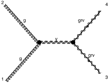
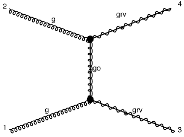
(a)                                      (b)

Figure 1: The relevant diagrams contributing to the fastest energy growth in the $gg\to\tilde{G}\tilde{G}$ process. They consist of an $s$-channel graviton exchange diagram (a) and $t,u$-channel gluino exchange diagrams (b).

Tree unitarity violation in the gravitino pair production process $gg\to\tilde{G}\tilde{G}$ has been studied by Bhattacharya and Roy in Ref. Bhattacharya:1988zp . In this section, we compare our numerical results with their approximated analytic results. There are three diagrams which contribute to the fastest energy growth in this process, an $s$-channel graviton exchange diagram and $t,u$-channel gluino exchange diagrams, as shown in Figure 1.

The relevant interaction Lagrangian is given by

$${\cal L}=-\frac{1}{2\overline{M}_{\rm Pl}}\overline{\Psi}_{\mu}\gamma^{\nu\rho}\gamma^{\mu}\lambda_{a}g^{a}_{\nu\rho}-\frac{1}{\overline{M}_{\rm Pl}}(T^{\mu\nu}_{g}+T^{\mu\nu}_{\tilde{G}})G_{\mu\nu},$$ (14)

where $\Psi_{\mu}$ is the spin-$\frac{3}{2}$ gravitino field, $\lambda_{a}$ the gluino field, and $g^{a}_{\mu\nu}$ the field strength tensor for a gluon $g^{a}_{\mu}$. We also recall that our conventions on the generators of the Lorentz algebra in the spinorial representation $\gamma^{\mu\nu}$ are defined in Appendix A. Moreover, $\overline{M}_{\rm Pl}\equiv M_{\rm Pl}/\sqrt{8\pi}\sim 2.4\times 10^{18}$ GeV denotes the reduced Planck mass. The first term in the Lagrangian of Eq. (14) has been extracted from the complete set of gravitino interactions as described in Section 3.1, whereas its second term describes the interactions of a spin-2 graviton $G_{\mu\nu}$ with gluons deAquino:2011ix and gravitinos. It shows the well-known feature that a spin-2 graviton couples to other fields via their energy-momentum tensor, $T_{g}^{\mu\nu}$ and $T_{\tilde{G}}^{\mu\nu}$ in the gluon and gravitino cases, respectively. Those two last quantities are given by

$$\begin{split}T_{g}^{\mu\nu}=&\ \frac{1}{4}\eta^{\mu\nu}g_{a}^{\rho\sigma}g^{a}_{\rho\sigma}-g^{a,\mu}_{\rho}g_{a}^{\nu\rho}\\ &\ -\frac{1}{\xi}\eta^{\mu\nu}\big{\{}g^{a}_{\rho}\,\partial^{\rho}\partial^{\sigma}g_{a,\sigma}+\frac{1}{2}(\partial^{\rho}g^{a}_{\rho})(\partial^{\sigma}g_{a,\sigma})\big{\}}\\ &\ +\frac{1}{\xi}\left(g^{a,\mu}\partial^{\nu}\partial^{\rho}g_{a,\rho}+g^{a,\nu}\partial^{\mu}\partial^{\rho}g_{a,\rho}\right)\ ,\\ T^{\mu\nu}_{\tilde{G}}=&\ \frac{1}{8}\epsilon^{\lambda\rho\sigma\mu}\overline{\Psi}_{\lambda}\gamma^{5}\gamma^{\nu}\overleftrightarrow{{\partial}_{\sigma}}\Psi_{\rho}+(\mu\leftrightarrow\nu)\\ &\ -\frac{i}{8}\epsilon^{\lambda\rho\sigma\mu}\partial_{\tau}(\overline{\Psi}_{\lambda}\gamma^{5}\{\gamma_{\sigma},\gamma^{\nu\tau}\}\Psi_{\rho})+(\mu\leftrightarrow\nu)\\ &\ -im_{3/2}\overline{\Psi}_{\lambda}(\eta^{\mu\nu}\gamma^{\lambda\rho}-\eta^{\rho\nu}\gamma^{\lambda\mu}-\eta^{\rho\mu}\gamma^{\lambda\nu})\Psi_{\rho}\ ,\end{split}$$ (15)

where the dependence on the gauge fixing parameter $\xi$ in the gluon energy-momentum tensor has been kept explicit although we adopt Feynman gauge, i.e., $\xi=1$, in the rest of this section. Moreover, the operator $\overleftrightarrow{\partial_{\sigma}}$ stands for the usual Hermitian derivative operator,

$$\overline{\Psi}_{\lambda}\cdots\overleftrightarrow{\partial}_{\sigma}\Psi_{\rho}=\overline{\Psi}_{\lambda}\cdots\partial_{\sigma}\Psi_{\rho}-\left(\partial_{\sigma}\overline{\Psi}_{\lambda}\right)\cdots\Psi_{\rho}\ .$$ (16)

To validate our gravitino implementation, we compute explicitly the helicity amplitudes ${\cal M}_{\lambda_{1}\lambda_{2},\lambda_{3}\lambda_{4}}$ associated with the process

$$g(p_{1},\lambda_{1})+g(p_{2},\lambda_{2})\to\tilde{G}(p_{3},\lambda_{3})+\tilde{G}(p_{4},\lambda_{4})\ .$$ (17)

They are presented in Appendix C. We then select a particular helicity combination and choose to investigate the properties of the ${\cal M}_{1,-1,\frac{1}{2},-\frac{1}{2}}$ amplitude, as it gives rise to the leading energy growth with the partonic center-of-mass (CM) energy $\sqrt{s}$. Expanding the $s$-, $t$- and $u$-channel contributions to the considered amplitudes in terms of the gravitino mass, one gets

$$\begin{split}{\mathcal{M}}^{s}=&\ -\frac{s}{12\overline{M}_{\rm Pl}^{2}}(1+c_{\theta})s_{\theta}\Big{[}\frac{s}{m^{2}_{3/2}}+4\Big{]}+{\cal O}(m_{3/2}^{2})\ ,\\ {\mathcal{M}}^{t}=&\ \frac{s}{6\overline{M}_{\rm Pl}^{2}x_{t}}s^{3}_{\theta}+{\cal O}(m_{3/2}^{2})\ ,\\ {\mathcal{M}}^{u}=&\ \frac{s}{24\overline{M}_{\rm Pl}^{2}x_{u}}(1+c_{\theta})^{2}s_{\theta}\Big{[}\frac{s}{m^{2}_{3/2}}+1+\frac{1}{x_{u}}(1+c_{\theta})\Big{]}\\ &\quad+{\cal O}(m_{3/2}^{2})\ ,\end{split}$$ (18)

following the notations of Appendix C, and where $s_{\theta}$ and $c_{\theta}$ stand for the sine and cosine of the scattering angle $\theta$ defined as the angle between the $\mathbf{p}_{1}$ and $\mathbf{p}_{3}$ directions in the partonic center-of-mass frame. We also introduce the reduced variables $x_{t,u}=\frac{m_{\tilde{g}}^{2}}{s}+\frac{1}{2}(1\mp c_{\theta})$. In the limit of large center-of-mass energies, or equivalently when $m_{\tilde{g}}/\sqrt{s}\to 0$, the $s^{2}$ energy growth behavior of the $s$- and $u$-channel diagrams cancels,

$$\begin{split}{\mathcal{M}}_{1,-1,\frac{1}{2},-\frac{1}{2}}\to-\frac{s}{6\overline{M}_{\rm Pl}^{2}}s_{\theta}\Big{[}\frac{m_{\tilde{g}}^{2}}{m_{3/2}^{2}}\!-\!\frac{3}{2}(1\!+\!c_{\theta})\Big{]}\!+\!{\cal O}(m_{3/2}^{2})\ ,\end{split}$$ (19)

whereas the linear $s$-dependence still remains Bhattacharya:1988zp .

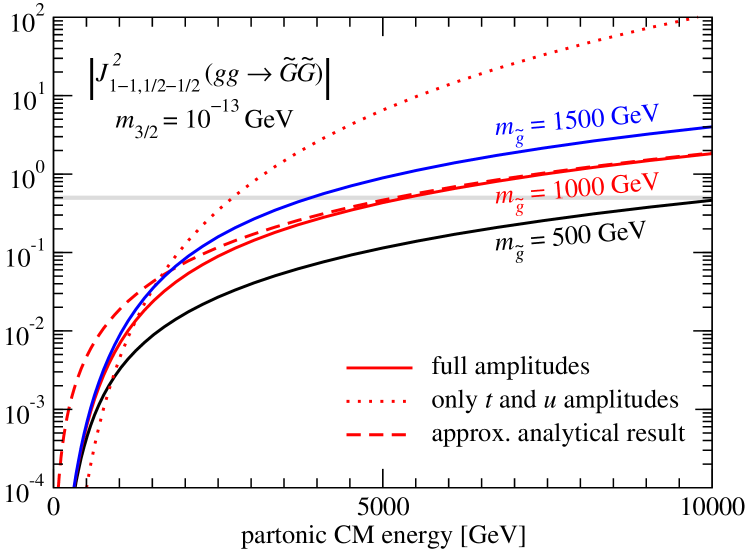
Figure 2: Energy dependence of the projected partial wave amplitude $\big{|}J^{2}_{1-1,\frac{1}{2}-\frac{1}{2}}\big{|}$ defined in Eq. (20) for the $gg\to\tilde{G}\tilde{G}$ process and for different choices of the gluino mass. The solid lines are calculated by MadGraph 5 and use the full amplitude. For the $m_{\tilde{g}}=1000$ GeV case, we also show the analytical results in the $\sqrt{s}\gg m_{3/2},m_{\tilde{g}}$ limit of Ref. Bhattacharya:1988zp (dashed) as well as the $s^{2}$ dependence resulting from the $t$- and $u$-channel diagram contributions only (dotted).

One of the advantages of our implementation consists of flexibility, i.e., one can vary parameters in the entire model parameter space and efficiently produce the related results. Figure 2 hence illustrates the energy dependence of the projected partial wave amplitude,

$$J^{2}_{1,-1,\frac{1}{2},-\frac{1}{2}}=\frac{1}{32\pi}\int_{-1}^{1}{\rm d}\cos\theta\,d^{2}_{21}(\theta)\,{\cal M}_{1,-1,\frac{1}{2},-\frac{1}{2}}\ ,$$ (20)

for different gluino masses. In this expression, we introduce the $J=2$ Wigner $d$-function $d^{2}_{21}(\theta)$ (see Appendix B.5). The analytic result of Eq. (19) (dashed line) is derived in the $\sqrt{s}\gg m_{3/2},m_{\tilde{g}}$ limit Bhattacharya:1988zp and agree with our numerical predictions calculated by MadGraph 5 in the high-energy region where this approximation is valid. In contrast, in the low-energy regime, the sub-leading term to Eq. (19) in the $m^{2}_{\tilde{g}}/s$ expansion becomes relevant, and one observes the deviation of the approximated analytical result from our numerical predictions. Finally, partial wave unitarity requires

$$\big{|}J^{2}_{1,-1,\frac{1}{2},-\frac{1}{2}}\big{|}<\frac{1}{2}\ ,$$ (21)

which is shown by a gray line on the figure.

We note that, in the $\sqrt{s}\gg m_{3/2}$ limit, goldstino-gravitino equivalence allows us to replace the spin-$\frac{3}{2}$ gravitino by the spin-$\frac{1}{2}$ goldstino (which we denote by $\chi$), $\Psi_{\mu}\sim\sqrt{2/3}\,\partial_{\mu}\chi/m_{3/2}$. We have verified that we obtain results similar to those of Figure 2 in this case.

4.1.2 Gluino pair-production

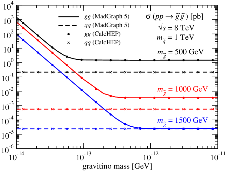
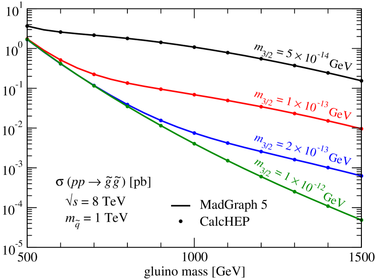
Figure 3: Total cross sections for gluino pair-production at the LHC, running at a center-of-mass energy of 8 TeV, presented as a function of the gravitino mass (upper panel) and of the gluino mass (lower panel). Squark masses are fixed to 1 TeV.

We now turn to the analysis of the $t,u$-channel gravitino contributions to gluino pair-production when the final state arises from gluon scattering Dicus:1989gg ; Kim:1997iwa .

In Figure 3, we present the different contributions to the total cross section for gluino pair-production $pp\to\tilde{g}\tilde{g}$ at the LHC, running at a center-of-mass energy of 8 TeV. In the upper panel of the figure, we fix the squark masses to 1 TeV and investigate the dependence of the cross section on the gravitino mass, for several choices of the gluino mass. The solid lines refer to the contribution from gluon scattering while the dashed lines are related to the quark-antiquark one. The gravitino diagrams contribute significantly only when the gravitino is very light with respect to the gluino mass. In other words, when $m_{3/2}\lesssim 6\cdot 10^{-14}$ GeV, $3\cdot 10^{-13}$ GeV, and $7\cdot 10^{-13}$ GeV for a gluino of 500 GeV, 1000 GeV and 1500 GeV, respectively.

In the lower panel of Figure 3, we analyze the dependence of the total cross section on the gluino mass for squark masses of 1 TeV and various values of the gravitino mass. This illustrates the scaling of the cross section in $1/m^{4}_{3/2}$ in the parameter space regions where gravitino diagrams dominate the cross section.

4.2 Top-quark excitation

Among the large number of new physics theories, those constructed upon the idea of compositeness of the Standard Model quarks and leptons usually predict the existence of both spin-$\frac{1}{2}$ and spin-$\frac{3}{2}$ states Burges:1983zg ; Kuhn:1984rj ; Kuhn:1985mi ; Moussallam:1989nm ; Almeida:1995yp ; Dicus:1998yc ; Walsh:1999pb ; Cakir:2007wn ; Stirling:2011ya ; Dicus:2012uh ; Hassanain:2009at . Since the top quark, by its large mass, is expected to play an important role in many new physics models, we only focus, in the following, on the description of an excited spin-$\frac{3}{2}$ top sector.

The dynamics of such a top quark excitation, represented by a four-component Rarita-Schwinger field $\Psi_{\mu}$ of mass $M$, is described by supplementing to the Standard Model Lagrangian ${\cal L}_{\rm SM}$ the gauge-covariant version of the Lagrangian of Eq. (114),

$${\cal L}={\cal L}_{\rm SM}+\epsilon^{\mu\nu\rho\sigma}\bar{\Psi}_{\mu}\gamma_{5}\gamma_{\sigma}D_{\nu}\Psi_{\rho}+2iM{\bar{\Psi}}_{\mu}\gamma^{\mu\nu}\Psi_{\nu}\ ,$$ (22)

the spacetime derivative having been replaced by the gauge covariant derivative

$$D_{\mu}\Psi_{\nu}=\partial_{\mu}\Psi_{\nu}-ig_{s}T_{a}\Psi_{\nu}g_{\mu}^{a}\ .$$ (23)

In this expression, we introduce the QCD coupling constant ($g_{s}$) and the fundamental representation matrices of $SU(3)$ ($T_{a}$). We also denote the gluon field by $g_{\mu}^{a}$, as in Section 4.1. Mixing of the spin-$\frac{3}{2}$ top excitation in general occurs through dimension-five operators suppressed by a new physics energy scale $\Lambda$. Although there are several ways to describe such a mixing, we assume it, for the sake of the example, agnostic of the left-handedness or right-handedness of the spin-$\frac{1}{2}$ top quark $t$ and embed the relevant interactions within the Lagrangian

$${\cal L}_{5}=i\frac{g_{s}}{\Lambda}\bar{\Psi}_{\rho}\Big{[}\eta^{\rho\mu}+z\gamma^{\rho}\gamma^{\mu}\Big{]}\gamma^{\nu}T_{a}t\ g_{\mu\nu}^{a}+{\rm h.c.}\ ,$$ (24)

We leave, in the following, the off-shell parameter $z$ free.

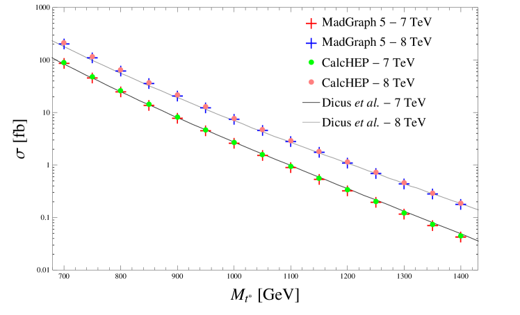
Figure 4: Total cross section for the production of an excited top quark pair at the LHC, for a center-of-mass energy of 7 TeV (red crosses and green circles) and 8 TeV (blue crosses and red circles), as a function of the excited top mass $M_{t^{*}}$. We compare predictions obtained by means of MadGraph 5 (crosses) and CalcHep (circles) to the analytical formulas presented in Ref. Dicus:2012uh (lines).

4.2.1 Top-quark excitation pair-production

In order to validate our implementation in the simulation chain mentioned in Section 3, we first focus on the pair production of spin-$\frac{3}{2}$ top excitations at the LHC, vetoing diagrams involving a top quark. We compare in Figure 4 predictions derived from the analytical formulas presented in Ref. Dicus:2012uh to results obtained by means of the MadGraph 5 and CalcHep event generators. The relevant model files have been produced by implementing the Lagrangians of Eqs. (22) and (24) into FeynRules and exporting the associated Feynman rules to a UFO library to be used with MadGraph 5 and to a CalcHep model. We consider the LHC collider running at a center-of-mass energy of 7 TeV and 8 TeV and convolve the associated squared matrix element with the leading order fit of the CTEQ6 parton densities Pumplin:2002vw after setting both unphysical factorization and renormalization scales to the mass of the top excitation $M_{t^{*}}$. All calculations fully agree, and the usual behavior of a cross section smoothly falling with an increasing top-$\frac{3}{2}$ mass is observed. From these results, it is found that spin-$\frac{3}{2}$ excitations of the top quark with masses $M_{t^{*}}\lesssim 1$ TeV could have been copiously pair-produced at both past LHC runs. Additionally, we have compared the symbolic calculations performed by CalcHEP to the explicit analytic formulas given in Ref. Dicus:2012uh and found perfect agreement.

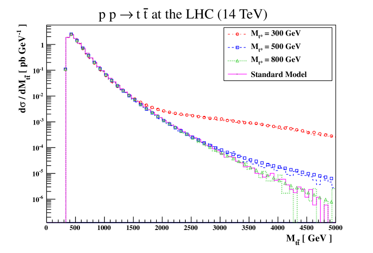
Figure 5: Invariant-mass spectrum of a top-antitop pair as would be produced at the LHC, running at a center-of-mass energy of 14 TeV, for an excited top mass of $M_{t^{*}}=300$ GeV (red dashed-dotted line), 500 GeV (blue dashed line) and 800 GeV (green dotted line) and in the context of the Standard Model (plain purple line). The dashed lines were obtained from MadGraph 5 while the circles, boxes and triangles were obtained from CalcHEP.

4.2.2 Top-quark pair-production

Next, mixing effects of spin-$\frac{1}{2}$ and spin-$\frac{3}{2}$ top states are investigated in the framework of the production of a (spin-$\frac{1}{2}$) top-antitop quark pair at the LHC, running at a center-of-mass energy of 14 TeV. In the presence of new physics as described by the Lagrangians of Eqs. (22) and (24), two additional $t$-channel and $u$-channel diagrams lead to the production of a top-antitop final state via the exchange of a spin-$\frac{3}{2}$ top partner from a gluon-gluon initial state. Fixing first the off-shell parameter to $z=0$ and the new physics scale to $\Lambda=7M_{t^{*}}$, we study the variation of the differential cross section ${\rm d}\sigma/{\rm d}M_{t\bar{t}}$ with the mass of the spin-$\frac{3}{2}$ excitation $M_{t^{*}}$ in Figure 5. Generating events with the MadGraph 5 program after fixing both unphysical scales to the top mass $M_{t}=173$ GeV, differential distributions are then extracted with the MadAnalysis 5 package Conte:2012fm and compared to those generated using the CalcHEP package and its internal histogramming routine. We recover earlier results Stirling:2011ya and show excesses with respect to the pure Standard Model case at large top-antitop invariant masses. For the three scenarios with a respective excited top mass of 300 GeV, 500 GeV and 800 GeV, respectively, new physics effects appear once the effective scale $\Lambda$ threshold is crossed, i.e., where the theory becomes unreliable and unitarity is violated. A proper treatment would require, e.g., the introduction of form factors as in Ref. Moussallam:1989nm . This however goes beyond the scope of this work devoted to an illustration of the implementation of spin-$\frac{3}{2}$ fields in automated high-energy physics tools.

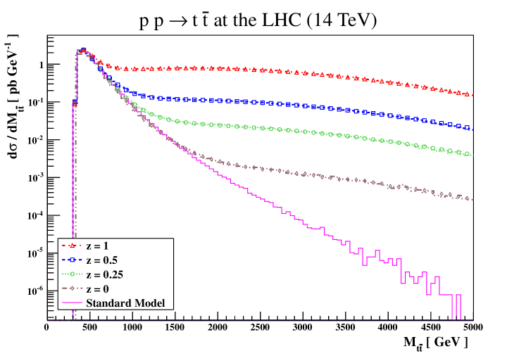
Figure 6: Invariant-mass spectrum of a top-antitop pair as would be produced at the LHC, running at a center-of-mass energy of 14 TeV, for an excited top mass of $M_{t^{*}}=300$ GeV and an off-shell parameter fixed to $z=0$ (gray large dashed-dotted line), $z=0.25$ (green dotted line), $z=0.5$ (blue dashed line) and $z=1$ (red small dashed-dotted line). The results are confronted to the Standard Model predictions (plain purple line).

In Figure 6, we fix the top-excitation mass to $300$ GeV and study the importance of the $z$ parameter on the differential distribution ${\rm d}\sigma/{\rm d}M_{t\bar{t}}$ at the LHC, still assumed to be running at a center-of-mass energy of 14 TeV. Similarly to the findings of earlier works Stirling:2011ya , the off-shell parameter is found to largely control the shape of the $M_{t\bar{t}}$ distribution. For large positive $z$-values, new physics effects appear to be important even far below the effective scale $\Lambda$, in contrast to more popular choices where $z$ is taken vanishing or negative Kuhn:1984rj ; Moussallam:1989nm .

4.3 Angular distributions for a spin-$\mathbf{\frac{3}{2}}$ particle

In this section, we study a particular case of spin-$\frac{3}{2}$ colored resonances that can be thought of as excited quarks. We exploit our implementation to test spin correlation effects possibly due to such resonances. In the rest of this section, we use the notation $u^{*\mu}$ for Rarita-Schwinger fields describing excited spin-$\frac{3}{2}$ quarks with the same internal quantum numbers as the up quark, and $d^{*\mu}$ for Rarita-Schwinger fields with the same quantum numbers as the down quark. If these resonances existed, they could be produced in a proton-proton collider when one quark and one gluon scatter. The simplest gauge-invariant operator that can describe such a process is

$${\cal L}_{\text{prod}}=\frac{g_{s}}{\Lambda}g^{a}_{\mu\nu}\overline{q}\gamma^{\mu}(k_{-}P_{L}+k_{+}P_{R})T_{a}q^{*\nu}+{\rm h.c.}\ .$$ (25)

In this expression, the excited and usual quark fields are denoted by $q^{*}=(u^{*},d^{*})$ and $q=(u,d)$, $P_{L}$ and $P_{R}$ are chirality projectors acting on spin space, $\Lambda$ is a cut-off scale and the interaction strengths are described by the $k_{\pm}$ parameters. We recall that the objects related to strong interactions have been introduced in the two previous subsections. We assume now that the resonances decay into a quark and either a photon or a $Z$ boson. After electroweak symmetry breaking, the simplest Lagrangian describing these decays reads

$$\begin{split}{\cal L}_{\text{decay}}=&\ \frac{e}{\Lambda}F_{\mu\nu}\overline{q}(k_{\gamma-}P_{L}+k_{\gamma+}P_{R})\gamma^{\mu}q^{*\nu}+{\rm h.c.}\\ &\ +\dfrac{g}{\cos\theta_{W}}Z_{\mu}\overline{q}(k_{Z-}P_{L}+k_{Z+}P_{R})q^{*\mu}+{\rm h.c.}\ ,\end{split}$$ (26)

where we denote the photon field strength tensor by $F_{\mu\nu}$ and model the couplings by the parameters $k_{\gamma\pm}$ and $k_{Z\pm}$. In order to study the angular distribution in the decay products caused by these resonances, we calculate analytically the corresponding differential cross sections. For the process $gq\to q^{*}\to\gamma q$, we find

$$\begin{split}\frac{{\rm d}\sigma}{{\rm d}\Omega}\propto&\ \left(|k_{+}|^{2}|k_{\gamma+}|^{2}+|k_{-}|^{2}|k_{\gamma-}|^{2}\right)\left|d^{\frac{3}{2}}_{\mathtt{\frac{3}{2}\frac{3}{2}}}(\theta)\right|^{2}\\ &\ +\left(|k_{-}|^{2}|k_{\gamma+}|^{2}+|k_{+}|^{2}|k_{\gamma-}|^{2}\right)\left|d^{\frac{3}{2}}_{\mathtt{\frac{3}{2}-\frac{3}{2}}}(\theta)\right|^{2}\ ,\end{split}$$ (27)

while for the process $gq\to q^{*}\to Zq$, we have

$$\begin{split}\frac{{\rm d}\sigma}{{\rm d}\Omega}\propto&\ \left(|k_{+}k_{Z+}|^{2}+|k_{-}k_{Z-}|^{2}\right)\left|d^{\frac{3}{2}}_{\mathtt{\frac{3}{2}\frac{1}{2}}}(\theta)\right|^{2}\\ &\ +\left(|k_{+}k_{Z-}|^{2}+|k_{-}k_{Z+}|^{2}\right)\left|d^{\frac{3}{2}}_{\mathtt{\frac{3}{2}-\frac{1}{2}}}(\theta)\right|^{2}\\ &\ +\mathcal{O}\left(\frac{m_{Z}^{2}}{m^{2}}\right)\ .\end{split}$$ (28)

For these expressions, we have assumed that the energy in the center-of-mass frame equals the mass of the resonance $m$. That is, the spin-$\frac{3}{2}$ particle is on-shell. We see that expressing the scattering amplitudes in terms of the Wigner $d$-functions makes the angular dependence of our results more transparent. We have reviewed the Wigner $d$-functions in Appendix B.5 and give the relevant spin-$\frac{3}{2}$ Wigner $d$-functions in Table 1.

$m$	$m^{\prime}$	$d^{\frac{3}{2}}_{mm^{\prime}}(\theta)$
$\frac{1}{2}$	$\frac{1}{2}$	$\frac{1}{2}\left(3\cos\theta-1\right)\cos\frac{\theta}{2}$
$\frac{3}{2}$	$\frac{1}{2}$	$-\frac{\sqrt{3}}{2}\left(\cos\theta+1\right)\sin\frac{\theta}{2}$
$\frac{3}{2}$	$\frac{3}{2}$	$\frac{1}{2}\left(\cos\theta+1\right)\cos\frac{\theta}{2}$

Table 1: Wigner $d$-functions used in this paper. The expressions that are not listed are related to the ones shown in the table by means of Eq. (124).

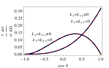
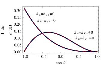
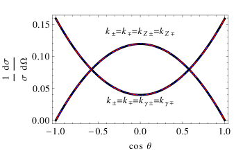
Figure 7: Angular distributions for three different choices of couplings. We show analytical results obtained from Eq. (27) and Eq. (28) (solid black) and numerical predictions of CalcHEP (dashed red) and MadGraph 5 (blue dotted).

We have implemented this new spin-$\frac{3}{2}$ particle along with the Lagrangian of Eq. (25) and Eq. (26) into FeynRules and exported the model to CalcHEP and MadGraph 5 using the interfaces described in the previous section. We have then generated events for the processes $gq\to q^{*}\to\gamma q$ and $gq\to q^{*}\to Zq$ for three different choices of couplings and show the resulting distributions in the three panels of Figure 7. The solid black curves correspond to the analytical computations of Eq. (27) and Eq. (28), while the red dashed and blue dotted predictions have been numerically obtained by using CalcHEP and MadGraph 5, respectively. In all cases, the results match perfectly, illustrating the on-shell propagation of a spin-$\frac{3}{2}$ particle. For this study, we used a new physics mass of 1 TeV and width of 1 GeV for the sake of the example, such a small relative width making the off-shell effects negligible.

5 Summary

In this paper, we have reported the implementation of support for spin-$\frac{3}{2}$ fields in the high-energy physics programs ALOHA, CalcHEP, FeynRules and MadGraph 5, including the definition of the conventions for those fields in the UFO format.

We have used the chain of packages above-mentioned for several physics applications. First, we have implemented the gravitino of supergravity together with its interactions in FeynRules and analyzed both gravitino pair-production and gravitino contributions to gluino pair-production at the LHC using MadGraph 5. Our numerical results have been compared to known analytic expressions that can be found in the literature and perfect agreement has been found. Next, we have implemented a spin-$\frac{3}{2}$ top-quark excitation into FeynRules and studied its pair production using both MadGraph 5 and CalcHEP. On the one hand, we have compared the resulting symbolic calculation of CalcHEP with previous analytic calculations. On the other hand, the numerical results obtained from both MadGraph 5 and CalcHEP have been confronted to the literature and we have studied the effects implied by the existence of a top spin-$\frac{3}{2}$ excitation on top-quark pair production. In all cases, we have found again a perfect agreement. Finally, we have implemented an effective operator for spin-$\frac{3}{2}$ colored resonances in FeynRules, analyzed the angular distributions in their $s$-channel production mechanism in both MadGraph 5 and CalcHEP and compared with analytic calculations involving the Wigner $d$-functions. Once again, the results have been found to match perfectly.

Appendix A Conventions

In this Appendix, we collect the conventions adopted in this manuscript. The metric is given by

$$\eta_{\mu\nu}=\mathrm{diag}(1,-1,-1,-1)\ ,$$ (29)

and the fully antisymmetric tensor of rank four is defined by $\epsilon_{0123}=1$. The four-vectors built upon the Pauli matrices are given by their usual form,

$$\sigma^{\mu}=\big{(}1,\sigma^{i}\big{)}\quad\text{and}\quad\bar{\sigma}^{\mu}=\big{(}1,-\sigma^{i}\big{)}\ ,$$ (30)

where the Pauli matrices $\sigma^{i}$ with $i=1,2,3$ read

$$\sigma^{1}=\begin{pmatrix}0&1\\ 1&0\end{pmatrix}\ ,\quad\sigma^{2}=\begin{pmatrix}0&-i\\ i&0\end{pmatrix}\ ,\quad\sigma^{3}=\begin{pmatrix}1&0\\ 0&-1\end{pmatrix}\ .$$ (31)

This allows to write the generators of the Lorentz algebra in the (two-component) left-handed and right-handed spinorial representations as

$$\sigma^{\mu\nu}=\frac{i}{4}\Big{(}\sigma^{\mu}{\bar{\sigma}}^{\nu}-\sigma^{\nu}{\bar{\sigma}}^{\mu}\Big{)}\quad\text{and}\quad{\bar{\sigma}}^{\mu\nu}=\frac{i}{4}\Big{(}{\bar{\sigma}}^{\mu}\sigma^{\nu}-{\bar{\sigma}}^{\nu}\sigma^{\mu}\Big{)}\ ,$$ (32)

respectively.

Moving to four-component spinors, Dirac matrices are defined in the Weyl representation by

$$\gamma^{\mu}=\begin{pmatrix}0&\sigma^{\mu}\\ \bar{\sigma}^{\mu}&0\end{pmatrix}\ ,$$ (33)

and span the Clifford algebra

$$\Big{\{}\gamma^{\mu},\gamma^{\nu}\Big{\}}=2\eta^{\mu\nu}\ .$$ (34)

Additionally, the fifth Dirac matrix $\gamma_{5}$ is given by

$$\gamma_{5}=i\gamma^{0}\gamma^{1}\gamma^{2}\gamma^{3}=\begin{pmatrix}-1&0\\ 0&1\end{pmatrix}\ .$$ (35)

The $\gamma$-matrices allow to build the generators of the Lorentz algebra in the four-component spinorial representation,

$$\gamma^{\mu\nu}=\frac{i}{4}\Big{(}\gamma^{\mu}\gamma^{\nu}-\gamma^{\nu}\gamma^{\mu}\Big{)}\ ,$$ (36)

as well as the quantity $\gamma^{\mu\nu\rho}$ which may appear in some specific forms of the Rarita-Schwinger Lagrangian used in the literature,

$$\begin{split}\gamma^{\mu\nu\rho}=&\ \frac{1}{6}\Big{[}\gamma^{\mu}\gamma^{\nu}\gamma^{\rho}+\gamma^{\nu}\gamma^{\rho}\gamma^{\mu}+\gamma^{\rho}\gamma^{\mu}\gamma^{\nu}\\ &\ \quad-\gamma^{\nu}\gamma^{\mu}\gamma^{\rho}-\gamma^{\mu}\gamma^{\rho}\gamma^{\nu}-\gamma^{\rho}\gamma^{\nu}\gamma^{\mu}\Big{]}\ .\end{split}$$ (37)

The $\gamma^{\mu\nu}$ and $\gamma^{\mu\nu\rho}$ objects obey the important relations,

$$\epsilon^{\mu\nu\rho\sigma}\gamma_{5}\gamma_{\sigma}=-i\gamma^{\mu\nu\rho}\quad\text{and}\quad\epsilon^{\mu\nu\rho\sigma}\gamma_{\mu\nu}\gamma_{5}=2i\gamma^{\rho\sigma}\ ,$$ (38)

helpful to prove the equivalence between all the spin-$\frac{3}{2}$ Lagrangian forms employed up to now.

Appendix B Review of spin

In this appendix, we follow the approach of Weinberg to build up the properties of a spin-$\frac{3}{2}$ particle Weinberg:1995mt . The spin of a particle determines its polarization vectors, the latter determining its propagation on-shell. Off-shell, the propagator can have further dependence which vanishes on-shell. Moreover, the on-shell propagator is related to the on-shell quadratic part of the Lagrangian whereas the off-shell pieces of the propagator match the model-dependent off-shell quadratic terms of the Lagrangian. We begin with a discussion on spin.

Both the vacuum and the dynamics of quantum field theory are symmetric under the Lorentz group, whose algebra $\mathfrak{so}(3,1)$ is isomorphic to $\mathfrak{sl}(2,\mathbb{R})\oplus\overline{\mathfrak{sl}(2,\mathbb{R})}$, the representations of the two $\mathfrak{sl}(2,\mathbb{R})$ denoting the left-handed and right-handed chiral algebras. However, the four-momentum of the particles are further invariant under a subalgebra, called the little algebra. For a massive particle, this is easiest to see in the rest frame where its momentum is $p^{\mu}=(M,0,0,0)$. Any Lorentz transformation that is a pure rotation in space leaves invariant a massive particle at rest. As a result, the little algebra for a massive particle is $\mathfrak{so}(3)$, the algebra of spatial rotations, which is isomorphic to $\mathfrak{su}(2)$, and each massive particle is classified according to its transformation properties under this little algebra or, in other words, according to its “spin”. This little algebra is the diagonal subalgebra of the left and right chiral Lorentz algebras, $\mathfrak{sl}(2,\mathbb{R})$ and $\overline{\mathfrak{sl}(2,\mathbb{R})}$. As a result, if a field transforms under the $(a,b)$ representation of the Lorentz algebra, it has a spin between $a+b$ and $|a-b|$.

As is well known, a scalar field transforms as $(0,0)$ under the Lorentz algebra and is, therefore, a spin-$0$ field. Ordinary matter fermions transform as either $(\frac{1}{2},0)$ or $(0,\frac{1}{2})$ and are, therefore, spin-$\frac{1}{2}$ particle. Vector fields transform as $(\frac{1}{2},\frac{1}{2})$ and contain both a spin-$1$ and a spin-$0$ piece. On-shell, the spin-$0$ field is removed by $\partial_{\mu}V^{\mu}=0$. Rarita-Schwinger fields $\Psi^{\mu}$ are formed as a direct product of $(\frac{1}{2},0)$ or $(0,\frac{1}{2})$ and $(\frac{1}{2},\frac{1}{2})$. Under the Lorentz symmetry, this contains

• $(0,\frac{1}{2})$ or $(\frac{1}{2},0)$ parts which are spin-$\frac{1}{2}$ fields and are removed by the on-shell equation $\gamma_{\mu}\Psi^{\mu}=0$;

• $(1,\frac{1}{2})$ or $(\frac{1}{2},1)$ parts which contain both the spin-$\frac{3}{2}$ field that we are after and another spin-$\frac{1}{2}$ field which is removed by the on-shell equation $\partial_{\mu}\Psi^{\mu}=0$.

Higher spin states are formed in a similar way.

In the rest of this appendix, we review the spin algebra $\mathfrak{su}(2)$ (Section B.1), the polarization vectors (Section B.2), the propagators (Section B.3), the quadratic Lagrangian terms (Section B.4), and finally the Wigner $d$-functions (Section B.5). Further, for the rest of this Appendix, we consider particles which are not self-charge-conjugate. The special case when particles are self-conjugate can be recovered from our results by replacing antiparticle states by charge conjugates of the particle states.

B.1 Spin: $\mathbf{\mathfrak{so(3)}\sim\mathfrak{su(2)}}$

We begin by reviewing what it means to be a representation of the $\mathfrak{su}(2)$ spin algebra. By definition, in this algebra there are three generators that satisfy the commutator rule

$$\left[J_{i},J_{j}\right]=i\epsilon_{ijk}J_{k}\ .$$ (39)

Two of these generators can be combined to form the raising/lowering operators,

$$J_{\pm}=J_{1}\pm iJ_{2}\ ,$$ (40)

which fulfill the commutator rules

$$\left[J_{+},J_{-}\right]=2J_{3}\quad\text{and}\quad\left[J_{3},J_{\pm}\right]=\pm J_{\pm}\ .$$ (41)

These can easily be checked by means of Eq. (39). With these definitions, it is easy to show that the effects of the raising/lowering operators on a state of spin $j$ represented by $|j,\sigma\rangle$ is to increase/decrease the eigenvalue of $J_{3}$ denoted by $\sigma$,

$$J_{3}J_{\pm}|j,\sigma\rangle=(\sigma\pm 1)J_{\pm}|j,\sigma\rangle\ .$$ (42)

A couple of general remarks are in order before we consider specific spin. Given the above definitions, we can easily see that the set of generators given by flipping the signs of all the generators and by switching $J_{+}$ with $J_{-}$ also forms a representation of the same algebra. We will show this by defining

$$\bar{J}_{3}=-J_{3}\quad\text{and}\quad\bar{J}_{\pm}=-J_{\mp}\ .$$ (43)

With these, we easily obtain

$$\left[\bar{J}_{+},\bar{J}_{-}\right]=2\bar{J}_{3}\quad\text{and}\quad\left[\bar{J}_{3},\bar{J}_{\pm}\right]=\pm\bar{J}_{\pm}\ .$$ (44)

This representation is called the complex representation and is very important in what follows. It finds its name due to the property

$$\left[-J^{*}_{i},-J^{*}_{j}\right]=i\epsilon_{ijk}\left(-J^{*}_{k}\right)\ .$$ (45)

Since we are taking our states as eigenvectors of $J_{3}$, this representation is diagonal and real (the eigenvalues of a Hermitian operator are real), so that $\bar{J}_{3}=-J_{3}^{*}=-J_{3}$. Further, in this basis, $J_{1}$ is real and symmetric while $J_{2}$ is imaginary and antisymmetric, so $\bar{J}_{1}=-J^{*}_{1}=-J_{1}$ and $\bar{J}_{2}=-J^{*}_{2}=J_{2}$. As a result, $\bar{J}_{\pm}=\left(-J^{*}_{1}\right)\pm i\left(-J^{*}_{2}\right)=-\left(J_{1}\mp iJ_{2}\right)=-J_{\mp}$.

Moreover, these raising/lowering operators can always be shifted by a phase and still satisfy the algebra. For example, if we define

$$J_{\pm}^{\prime}=e^{\pm i\phi}J_{\pm}\ ,$$ (46)

it is easy to show that

$$\left[J_{+}^{\prime},J_{-}^{\prime}\right]=2J_{3}\quad\text{and}\quad\left[J_{3},J_{\pm}^{\prime}\right]=\pm J_{\pm}^{\prime}\ .$$ (47)

So that the set $J_{3}$ with $J_{\pm}^{\prime}$ also forms a representation of $\mathfrak{su}(2)$. This will be important for understanding the Helas conventions for the spin-$\frac{1}{2}$ polarization vectors.

For the rest of this section, we consider the particle or antiparticle to have a mass $M$ and a four-momentum

$$p^{\mu}=\left(E,|\vec{p}|\sin\theta\cos\phi,|\vec{p}|\sin\theta\sin\phi,|\vec{p}|\cos\theta\right)$$ (48)

B.2 Polarization vectors

The polarization vectors for a particle $u$ and its antiparticle $v$ are determined by the spin of the particle. They transform under the spin representation of the particle and antiparticle, respectively, which is to say, the particle’s spin transforms according to $\vec{J}$ while the antiparticle’s spin transforms according to $-\vec{J}^{*}$. On the other hand, they both transform according to the same representation of the Lorentz algebra whose generators are $\vec{\mathcal{J}}$. For the rest of this discussion, we will take $J_{3}$ to measure the component of spin along the direction of motion. In other words, we will take $J_{3}$ to be the helicity operator. $J_{1}$ and $J_{2}$ will be defined appropriately, with the direction $1$ and $2$ orthogonal to direction $3$ and each other and satisfying Eq. (39).

As we mentioned, the spin algebra is a subalgebra of the Lorentz algebra. So, each spin transformation corresponds with a Lorentz transformation. For particles, we can write this as

$$\begin{split}J^{j}_{3}u_{\ell}(j,\sigma)=&\ \mathcal{J}^{(3)}_{\ell,\ell^{\prime}}u_{\ell^{\prime}}(j,\sigma)=\sigma u_{\ell}(j,\sigma)\ ,\\ J^{j}_{\pm}u_{\ell}(j,\sigma)=&\ \mathcal{J}^{(\pm)}_{\ell,\ell^{\prime}}u_{\ell^{\prime}}(j,\sigma)\\ =&\ \sqrt{(j\mp\sigma)(j\pm\sigma+1)}u_{\ell}(j,\sigma\pm 1)\ ,\end{split}$$ (49)

where $\ell$ and $\ell^{\prime}$ are the field indices under the Lorentz transformations and $\ell^{\prime}$ is summed over. Furthermore, we have assumed a trivial phase for the raising and lowering operators. Other phase choices are discussed later. Antiparticles transform according to the same representation of the Lorentz algebra and, so, we use the same $\vec{\mathcal{J}}$ operators. However, their spin transforms under the conjugate representation. As a result, the Lorentz transformations that were used for particles have the following effect on antiparticles,

$$\begin{split}-\bar{J}^{j}_{3}v_{\ell}(j,\sigma)=&\ \mathcal{J}^{(3)}_{\ell,\ell^{\prime}}v_{\ell^{\prime}}(j,\sigma)=-\sigma v_{\ell}(j,\sigma)\ ,\\ -\bar{J}^{j}_{\mp}v_{\ell}(j,\sigma)=&\ \mathcal{J}^{(\pm)}_{\ell,\ell^{\prime}}v_{\ell^{\prime}}(j,\sigma)\\ =&\ -\sqrt{(j\pm\sigma)(j\mp\sigma+1)}v_{\ell}(j,\sigma\mp 1)\ .\end{split}$$ (50)

For the rest of this subsection, we review the polarization vectors for spin-$\frac{1}{2}$, spin-$1$, spin-$\frac{3}{2}$, and spin-$2$ fields. We use the Helas convention for the spin-$\frac{1}{2}$ and spin-$1$ polarization vectors and show that they satisfy the spin algebra and derive any relevant phases in the raising and lowering operators. We then construct the spin-$\frac{3}{2}$ and spin-$2$ polarization vectors from these.

B.2.1 Spin-$\frac{1}{2}$ fields

According to the Helas conventions, the spin-$\frac{1}{2}$ polarization vectors are given by

$$\begin{split}u_{+1/2}(p)=&\ \left(\begin{array}[]{c}\sqrt{E-|\vec{p}|}\left(\begin{array}[]{c}\cos\frac{\theta}{2}\\ \sin\frac{\theta}{2}e^{i\phi}\end{array}\right)\\ \sqrt{E+|\vec{p}|}\left(\begin{array}[]{c}\cos\frac{\theta}{2}\\ \sin\frac{\theta}{2}e^{i\phi}\end{array}\right)\end{array}\right)\ ,\\ u_{-1/2}(p)=&\ \left(\begin{array}[]{c}\sqrt{E+|\vec{p}|}\left(\begin{array}[]{c}-\sin\frac{\theta}{2}e^{-i\phi}\\ \cos\frac{\theta}{2}\end{array}\right)\\ \sqrt{E-|\vec{p}|}\left(\begin{array}[]{c}-\sin\frac{\theta}{2}e^{-i\phi}\\ \cos\frac{\theta}{2}\end{array}\right)\end{array}\right)\ ,\\ v_{+1/2}(p)=&\ \left(\begin{array}[]{c}-\sqrt{E+|\vec{p}|}\left(\begin{array}[]{c}-\sin\frac{\theta}{2}e^{-i\phi}\\ \cos\frac{\theta}{2}\end{array}\right)\\ \sqrt{E-|\vec{p}|}\left(\begin{array}[]{c}-\sin\frac{\theta}{2}e^{-i\phi}\\ \cos\frac{\theta}{2}\end{array}\right)\end{array}\right)\ ,\\ v_{-1/2}(p)=&\ \left(\begin{array}[]{c}\sqrt{E-|\vec{p}|}\left(\begin{array}[]{c}\cos\frac{\theta}{2}\\ \sin\frac{\theta}{2}e^{i\phi}\end{array}\right)\\ -\sqrt{E+|\vec{p}|}\left(\begin{array}[]{c}\cos\frac{\theta}{2}\\ \sin\frac{\theta}{2}e^{i\phi}\end{array}\right)\end{array}\right)\ .\end{split}$$ (51)

We begin with the spin-$\frac{1}{2}$ form of the rotation and boost generators

$$\mathcal{J}_{i}=\frac{1}{2}\left(\begin{array}[]{cc}\sigma_{i}&0\\ 0&\sigma_{i}\end{array}\right)\quad\text{and}\quad\mathcal{K}_{i}=-\frac{i}{2}\left(\begin{array}[]{cc}\sigma_{i}&0\\ 0&-\sigma_{i}\end{array}\right)\ ,$$ (52)

where $\sigma_{i}$ denotes the Pauli matrices, and then combine $\mathcal{J}_{1}$ and $\mathcal{J}_{2}$ to form the ladder operators

$$\mathcal{J}_{\pm}=\mathcal{J}_{1}\pm i\mathcal{J}_{2}=\frac{1}{2}\left(\begin{array}[]{cc}\sigma_{1}\pm i\sigma_{2}&0\\ 0&\sigma_{1}\pm i\sigma_{2}\end{array}\right)\ .$$ (53)

We then rotate and boost from the particle rest frame to the laboratory frame of reference by employing the operator

$$\Lambda_{\frac{1}{2}}=$$ (54)

$$\quad\left(\begin{array}[]{cccc}e^{-\frac{\eta}{2}-i\frac{\phi}{2}}c_{\frac{\theta}{2}}&-e^{\frac{\eta}{2}-i\frac{\phi}{2}}s_{\frac{\theta}{2}}&0&0\\ e^{-\frac{\eta}{2}+i\frac{\phi}{2}}s_{\frac{\theta}{2}}&e^{\frac{\eta}{2}+i\frac{\phi}{2}}c_{\frac{\theta}{2}}&0&0\\ 0&0&e^{\frac{\eta}{2}-i\frac{\phi}{2}}c_{\frac{\theta}{2}}&-e^{-\frac{\eta}{2}-i\frac{\phi}{2}}s_{\frac{\theta}{2}}\\ 0&0&e^{\frac{\eta}{2}+i\frac{\phi}{2}}s_{\frac{\theta}{2}}&e^{-\frac{\eta}{2}+i\frac{\phi}{2}}c_{\frac{\theta}{2}}\end{array}\right)\ .$$ (59)

In this expression, we have introduced the sine and cosine of half the polar angle $c_{\theta/2}=\cos(\theta/2)$ and $s_{\theta/2}=\sin(\theta/2)$ as well as the pseudorapidity

$$\eta=\frac{1}{2}\ln\left(\frac{E+|\vec{p}|}{E-|\vec{p}|}\right)\ .$$ (60)

At the operator level, we hence get

$$\begin{split}\mathcal{J}^{(3)}=&\ \Lambda_{\frac{1}{2}}\mathcal{J}_{z}\Lambda_{\frac{1}{2}}^{-1}=\left(\begin{array}[]{cc}B&0\\ 0&B\end{array}\right)\ ,\\ \mathcal{J}^{(\pm)}=&\ \Lambda_{\frac{1}{2}}\mathcal{J}_{\pm}\Lambda_{\frac{1}{2}}^{-1}=\left(\begin{array}[]{cc}e^{\mp\eta}A_{\pm}&0\\ 0&e^{\pm\eta}A_{\pm}\end{array}\right)\ ,\end{split}$$ (61)

with

$$\begin{split}A_{\pm}=&\ \left(\begin{array}[]{cc}-\frac{1}{2}\sin\theta&\pm\frac{1}{2}\left(1\pm\cos\theta\right)e^{-i\phi}\\ \mp\frac{1}{2}\left(1\mp\cos\theta\right)e^{i\phi}&\frac{1}{2}\sin\theta\end{array}\right)\ ,\\ B=&\ \left(\begin{array}[]{cc}\frac{1}{2}\cos\theta&\frac{1}{2}\sin\theta e^{-i\phi}\\ \frac{1}{2}\sin\theta e^{i\phi}&-\frac{1}{2}\cos\theta\end{array}\right)\ .\end{split}$$ (62)

It can easily be shown that these operators satisfy the commutation properties of $\mathfrak{su}(2)$,

$$\left[\mathcal{J}^{(+)},\mathcal{J}^{(-)}\right]=2\mathcal{J}^{(3)}\quad\text{and}\quad\left[\mathcal{J}^{(3)},\mathcal{J}^{(\pm)}\right]=\pm\mathcal{J}^{(\pm)}\ .$$ (63)

They correspond with the helicity operator, raising operator and lowering operator in spin space for particles. We can explicitly check that they have the following effect on the particle polarization vectors of Eq. (51),

$$\begin{split}J^{1/2}_{3}u_{\pm 1/2}(p)=&\ \mathcal{J}^{(3)}u_{\pm 1/2}(p)=\pm\frac{1}{2}u_{\pm 1/2}(p)\ ,\\ J^{1/2}_{-}u_{1/2}(p)=&\ \mathcal{J}^{(-)}u_{1/2}(p)=e^{i\phi}u_{-1/2}(p)\ ,\\ J^{1/2}_{-}u_{-1/2}(p)=&\ \mathcal{J}^{(-)}u_{-1/2}(p)=0\ ,\\ J^{1/2}_{+}u_{-1/2}(p)=&\ \mathcal{J}^{(+)}u_{-1/2}(p)=e^{-i\phi}u_{1/2}(p)\ ,\\ J^{1/2}_{+}u_{1/2}(p)=&\ \mathcal{J}^{(+)}u_{1/2}(p)=0\ .\end{split}$$ (64)

From this, we learn that there is an extra phase associated with the ladder operators in the Helas conventions for spin-$\frac{1}{2}$,

$$J^{1/2}_{\pm}u_{\sigma}(p)=e^{\mp i\phi}\sqrt{\left(\frac{1}{2}\mp\sigma\right)\left(\frac{1}{2}\pm\sigma+1\right)}\ u_{\sigma\pm 1}(p)\ .$$ (65)

Since the generators formed in this way still form a representation of the spin algebra, this phase could have been absorbed into the definition of the polarization vectors.

For antiparticles, we find

$$\begin{split}\bar{J}^{1/2}_{3}v_{\pm 1/2}(p)=&\ -\mathcal{J}^{(3)}v_{\pm 1/2}(p)=\pm\frac{1}{2}v_{\pm 1/2}(p)\ ,\\ \bar{J}^{1/2}_{-}v_{1/2}(p)=&\ -\mathcal{J}^{(+)}v_{1/2}(p)=e^{-i\phi}v_{-1/2}(p)\ ,\\ \bar{J}^{1/2}_{-}v_{-1/2}(p)=&\ -\mathcal{J}^{(+)}v_{-1/2}(p)=0\ ,\\ \bar{J}^{1/2}_{+}v_{-1/2}(p)=&\ -\mathcal{J}^{(-)}v_{-1/2}(p)=e^{i\phi}v_{1/2}(p)\ ,\\ \bar{J}^{1/2}_{+}v_{1/2}(p)=&\ -\mathcal{J}^{(-)}v_{1/2}(p)=0\ ,\end{split}$$ (66)

and as a result,

$$\bar{J}^{1/2}_{\pm}v_{\sigma}(p)=e^{\pm i\phi}\sqrt{\left(\frac{1}{2}\mp\sigma\right)\left(\frac{1}{2}\pm\sigma+1\right)}\ v_{\sigma\pm 1}(p)\ .$$ (67)

B.2.2 Spin-$1$ fields

The polarization vectors associated with a spin-$1$ particle are given, following the Helas conventions, by

$$\begin{split}\epsilon^{\mu}_{+}(p)=&\ \frac{1}{\sqrt{2}}\left(\begin{array}[]{c}0\\ -\cos\theta\cos\phi+i\sin\phi\\ -\cos\theta\sin\phi-i\cos\phi\\ \sin\theta\end{array}\right)\ ,\\ \epsilon^{\mu}_{0}(p)=&\ \frac{1}{M}\left(\begin{array}[]{c}|\vec{p}|\\ E\sin\theta\cos\phi\\ E\sin\theta\sin\phi\\ E\cos\theta\end{array}\right)\ ,\\ \epsilon^{\mu}_{-}(p)=&\ \frac{1}{\sqrt{2}}\left(\begin{array}[]{c}0\\ \cos\theta\cos\phi+i\sin\phi\\ \cos\theta\sin\phi-i\cos\phi\\ -\sin\theta\end{array}\right)\ ,\end{split}$$ (68)

whereas those associated with a spin-$1$ antiparticle read

$$\begin{split}\bar{\epsilon}_{+}^{\mu}(p)=&\ \epsilon^{\mu*}_{+}(p)\ ,\\ \bar{\epsilon}_{0}^{\mu}(p)=&\ \epsilon^{\mu*}_{0}(p)\ ,\\ \bar{\epsilon}_{-}^{\mu}(p)=&\ \epsilon^{\mu*}_{-}(p)\ .\end{split}$$ (69)

In the vectorial representation, the spatial pieces of the rotation generators are given by

$$(\mathcal{J}_{i})^{j}{}_{k}=i\epsilon_{i}{}^{j}{}_{k}\ ,$$ (70)

where $\epsilon_{ijk}=1$ and $i$, $j$, $k$ = 1,2,3, while the time components are zero. On the other hand, the spatial components of the boost generators vanish while their time components are given by

$$(\mathcal{K}_{i})^{0}{}_{\mu}=i\eta_{i\mu}\quad\text{and}\quad(\mathcal{K}_{i})^{\mu}{}_{0}=-i\delta^{\mu}{}_{i}\ .$$ (71)

As a result, in the rest frame, we have

$$\begin{split}\mathcal{J}_{3}=\left(\begin{array}[]{cccc}0&0&0&0\\ 0&0&-i&0\\ 0&i&0&0\\ 0&0&0&0\end{array}\right)\quad\text{and}\quad\mathcal{J}_{\pm}=\left(\begin{array}[]{cccc}0&0&0&0\\ 0&0&0&\mp 1\\ 0&0&0&-i\\ 0&\pm 1&i&0\end{array}\right)\ .\end{split}$$ (72)

To get these generators in the laboratory frame of reference, we boost along the $z$-direction and rotate using

$$\Lambda_{1}=\left(\begin{array}[]{cccc}1&0&0&0\\ 0&c_{\phi}&-s_{\phi}&0\\ 0&s_{\phi}&c_{\phi}&0\\ 0&0&0&1\end{array}\right)\left(\begin{array}[]{cccc}1&0&0&0\\ 0&c_{\theta}&0&s_{\theta}\\ 0&0&1&0\\ 0&-s_{\theta}&0&c_{\theta}\end{array}\right)\frac{1}{M}\left(\begin{array}[]{cccc}E&0&0&p\\ 0&1&0&0\\ 0&0&1&0\\ p&0&0&E\end{array}\right)\ ,$$ (73)

where the sine and cosine of the azimuthal (polar) angle are denoted by $s_{\phi}$ ($s_{\theta}$) and $c_{\phi}$ ($c_{\theta}$). One can now derive the rotation generators

$$\begin{split}\mathcal{J}^{(3)}=&\ \Lambda_{1}\mathcal{J}_{3}\Lambda_{1}^{-1}=\left(\begin{array}[]{cccc}0&0&0&0\\ 0&0&-ic_{\theta}&is_{\theta}s_{\phi}\\ 0&ic_{\theta}&0&-is_{\theta}c_{\phi}\\ 0&-is_{\theta}s_{\phi}&is_{\theta}c_{\phi}&0\end{array}\right)\ ,\\ \mathcal{J}^{(\pm)}=&\ \Lambda_{1}\mathcal{J}_{\pm}\Lambda_{1}^{-1}\\ =&\ \left(\begin{array}[]{cccc}0&\frac{p}{M}C_{1\pm}&\frac{p}{M}C_{2\pm}&\mp\frac{ps_{\theta}}{M}\\ \frac{p}{M}C_{1\pm}&0&\frac{iEs_{\theta}}{M}&-\frac{E}{M}C_{3\pm}\\ \frac{p}{M}C_{2\pm}&-\frac{iEs_{\theta}}{M}&0&-\frac{E}{M}C_{4\pm}\\ \mp\frac{ps_{\theta}}{M}&\frac{E}{M}C_{3\pm}&\frac{E}{M}C_{4\pm}&0\end{array}\right)\ ,\end{split}$$ (74)

where we have introduced the quantities

$$\begin{split}C_{1\pm}=&\ \pm\cos\theta\cos\phi-i\sin\phi\ ,\\ C_{2\pm}=&\ \pm\cos\theta\sin\phi+i\cos\phi\ ,\\ C_{3\pm}=&\ -i\cos\theta\sin\phi\pm\cos\phi\ ,\\ C_{4\pm}=&\ i\cos\theta\cos\phi\pm\sin\phi\ .\end{split}$$ (75)

The commutators of these generators satisfy the usual relations,

$$\left[\mathcal{J}^{(+)},\mathcal{J}^{(-)}\right]=2\mathcal{J}^{(3)}\quad\text{and}\quad\left[\mathcal{J}^{(3)},\mathcal{J}^{(\pm)}\right]=\pm\mathcal{J}^{(\pm)}\ .$$ (76)

Acting on the spin-1 polarization vectors, we get

$$\begin{split}J_{3}\epsilon_{\pm}^{\mu}(p)=&\mathcal{J}^{(3)\mu}_{\hskip 14.45377pt\nu}\epsilon_{\pm}^{\nu}(p)=\pm\epsilon_{\pm}^{\mu}(p)\ ,\\ J_{3}\epsilon_{\pm}^{\mu}(p)=&\mathcal{J}^{(3)\mu}_{\hskip 14.45377pt\nu}\epsilon_{0}^{\nu}(p)=0\ ,\\ J_{-}\epsilon_{+}^{\mu}(p)=&\mathcal{J}^{(-)\mu}_{\hskip 18.06749pt\nu}\epsilon_{+}^{\nu}(p)=\sqrt{2}\epsilon_{0}^{\mu}(p)\ ,\\ J_{-}\epsilon_{0}^{\mu}(p)=&\mathcal{J}^{(-)\mu}_{\hskip 18.06749pt\nu}\epsilon_{0}^{\nu}(p)=\sqrt{2}\epsilon_{-}^{\mu}(p)\ ,\\ J_{-}\epsilon_{-}^{\mu}(p)=&\mathcal{J}^{(-)\mu}_{\hskip 18.06749pt\nu}\epsilon_{-}^{\nu}(p)=0\ ,\\ J_{+}\epsilon_{-}^{\mu}(p)=&\mathcal{J}^{(+)\mu}_{\hskip 18.06749pt\nu}\epsilon_{-}^{\nu}(p)=\sqrt{2}\epsilon_{0}^{\mu}(p)\ ,\\ J_{+}\epsilon_{0}^{\mu}(p)=&\mathcal{J}^{(+)\mu}_{\hskip 18.06749pt\nu}\epsilon_{0}^{\nu}(p)=\sqrt{2}\epsilon_{+}^{\mu}(p)\ ,\\ J_{+}\epsilon_{+}^{\mu}(p)=&\mathcal{J}^{(+)\mu}_{\hskip 18.06749pt\nu}\epsilon_{+}^{\nu}(p)=0\ ,\end{split}$$ (77)

so that we observe that no additional phase is required and the particle spin raising and lowering operators satisfy

$$J^{1}_{\pm}\epsilon_{\sigma}^{\mu}(p)=\sqrt{(1\mp\sigma)(1\pm\sigma+1)}\ \epsilon_{\sigma\pm 1}^{\mu}(p)\ .$$ (78)

For antiparticles, we find

$$\begin{split}\bar{J}_{3}\epsilon_{\pm}^{\mu*}(p)=&-\mathcal{J}^{(3)\mu}_{\hskip 14.45377pt\nu}\epsilon_{\pm}^{\nu*}(p)=\pm\epsilon_{\pm}^{\mu*}(p)\ ,\\ \bar{J}_{3}\epsilon_{\pm}^{\mu*}(p)=&-\mathcal{J}^{(3)\mu}_{\hskip 14.45377pt\nu}\epsilon_{0}^{\nu*}(p)=0\ ,\\ \bar{J}_{-}\epsilon_{+}^{\mu*}(p)=&-\mathcal{J}^{(+)\mu}_{\hskip 18.06749pt\nu}\epsilon_{+}^{\nu*}(p)=\sqrt{2}\epsilon_{0}^{\mu*}(p)\ ,\\ \bar{J}_{-}\epsilon_{0}^{\mu*}(p)=&-\mathcal{J}^{(+)\mu}_{\hskip 18.06749pt\nu}\epsilon_{0}^{\nu*}(p)=\sqrt{2}\epsilon_{-}^{\mu*}(p)\ ,\\ \bar{J}_{-}\epsilon_{-}^{\mu*}(p)=&-\mathcal{J}^{(+)\mu}_{\hskip 18.06749pt\nu}\epsilon_{-}^{\nu*}(p)=0\ ,\\ \bar{J}_{+}\epsilon_{-}^{\mu*}(p)=&-\mathcal{J}^{(-)\mu}_{\hskip 18.06749pt\nu}\epsilon_{-}^{\nu*}(p)=\sqrt{2}\epsilon_{0}^{\mu*}(p)\ ,\\ \bar{J}_{+}\epsilon_{0}^{\mu*}(p)=&-\mathcal{J}^{(-)\mu}_{\hskip 18.06749pt\nu}\epsilon_{0}^{\nu*}(p)=\sqrt{2}\epsilon_{+}^{\mu*}(p)\ ,\\ \bar{J}_{+}\epsilon_{+}^{\mu*}(p)=&-\mathcal{J}^{(-)\mu}_{\hskip 18.06749pt\nu}\epsilon_{+}^{\nu*}(p)=0\ ,\end{split}$$ (79)

which again shows us there is no extra phase associated with these polarization vectors. The raising and lowering operators satisfy in this case

$$\bar{J}^{1}_{\pm}\epsilon_{\sigma}^{\mu*}(p)=\sqrt{(1\mp\sigma)(1\pm\sigma+1)}\ \epsilon_{\sigma\pm 1}^{\mu*}(p)\ .$$ (80)

B.2.3 Spin-$\frac{3}{2}$ fields

The spin-$\frac{3}{2}$ polarization vectors can be formed as a direct product of the spin-$\frac{1}{2}$ and spin-$1$ polarization vectors. The generators are then simply the sum of those of the spin-$\frac{1}{2}$ and spin-$1$ representations,

$$J^{3/2}_{3}=J^{1/2}_{3}+J^{1}_{3}\quad\text{and}\quad J^{3/2}_{\pm}=J^{1/2}_{\pm}+J^{1}_{\pm}\ .$$ (81)

It is easily seen that these satisfy the $\mathfrak{su}(2)$ algebra.

We begin with the highest weight of the spin-$\frac{3}{2}$ representation which has helicity $\frac{3}{2}$ and is given by the product of the highest polarization of spin-$\frac{1}{2}$ and spin-$1$

$$u^{\mu}_{3/2,3/2}(p)=\epsilon^{\mu}_{+}(p)u_{+1/2}(p)\ .$$ (82)

We then lower the $J_{3}$-eigenvalue by using the $J^{3/2}_{-}$ operator to get the other states, $J^{1/2}_{-}$ only acting on spin-$\frac{1}{2}$ polarization vectors and $J^{1}_{-}$ on spin-$1$ polarization vectors. We now have the choice of the overall phase for the raising and lowering operators. We take the trivial choice with no additional phase,

$$J^{3/2}_{\pm}u^{\mu}_{3/2,\sigma}(p)=\sqrt{\left(\frac{3}{2}\mp\sigma\right)\left(\frac{3}{2}\pm\sigma+1\right)}\ u^{\mu}_{3/2,\sigma\pm 1}(p)\ .$$ (83)

We now work out the first step explicitly,

$$\begin{split}&J^{3/2}_{-}u^{\mu}_{3/2,3/2}(p)=\sqrt{3}u^{\mu}_{3/2,1/2}(p)\\ &\quad=\left(J^{1}_{-}\epsilon^{\mu}_{+}(p)\right)u_{+1/2}(p)+\epsilon^{\mu}_{+}\left(J^{1/2}_{-}u_{+1/2}(p)\right)\\ &\quad=\sqrt{2}\epsilon^{\mu}_{0}(p)u_{+1/2}(p)+e^{i\phi}\epsilon^{\mu}_{+}(p)u_{-1/2}(p)\ ,\end{split}$$ (84)

so that

$$u^{\mu}_{3/2,1/2}(p)=\sqrt{\frac{2}{3}}\epsilon^{\mu}_{0}(p)u_{+1/2}(p)+\frac{1}{\sqrt{3}}e^{i\phi}\epsilon^{\mu}_{+}(p)u_{-1/2}(p)\ .$$ (85)

Following the same procedure for the other states gives

$$\begin{split}u^{\mu}_{3/2,-1/2}(p)=&\ \sqrt{\frac{2}{3}}e^{i\phi}\epsilon^{\mu}_{0}(p)u_{-1/2}(p)\\ &\quad+\frac{1}{\sqrt{3}}\epsilon^{\mu}_{-}(p)u_{+1/2}(p)\ ,\\ u^{\mu}_{3/2,-3/2}(p)=&\ e^{i\phi}\epsilon^{\mu}_{-}(p)u_{-1/2}(p)\ .\end{split}$$ (86)

Antiparticle polarization vectors are derived in a similar fashion using the conjugate lowering operators and starting with the highest weight of the antiparticle polarization vector,

$$\begin{split}v^{\mu}_{3/2,3/2}(p)=&\ \epsilon^{\mu*}_{+}(p)v_{+1/2}(p)\ ,\\ v^{\mu}_{3/2,1/2}(p)=&\ \sqrt{\frac{2}{3}}\epsilon^{\mu*}_{0}(p)v_{+1/2}(p)\\ &\quad+\frac{1}{\sqrt{3}}e^{-i\phi}\epsilon^{\mu*}_{+}(p)v_{-1/2}(p)\ ,\\ v^{\mu}_{3/2,-1/2}(p)=&\ \sqrt{\frac{2}{3}}e^{-i\phi}\epsilon^{\mu*}_{0}(p)v_{-1/2}(p)\\ &\quad+\frac{1}{\sqrt{3}}\epsilon^{\mu*}_{-}(p)v_{+1/2}(p)\ ,\\ v^{\mu}_{3/2,-3/2}(p)=&\ e^{-i\phi}\epsilon^{\mu*}_{-}(p)v_{-1/2}(p)\ ,\end{split}$$ (87)

where we have again not included any extra phase in the raising and lowering operators.

B.2.4 Spin-$2$ fields

Just as in the case of the spin-$\frac{3}{2}$ fields, the spin-$2$ polarization vectors can be formed as the direct product of two spin-$1$ polarization vectors. The generators are hence the sum of the spin-$1$ generators for each polarization vector,

$$J^{2}_{3}=J^{1}_{3}+J^{1}_{3}\quad\text{and}\quad J^{2}_{\pm}=J^{1}_{\pm}+J^{1}_{\pm}\ ,$$ (88)

where it is understood that the first generator only acts on the first polarization vector and the second generator only acts on the second polarization vector. It is easily seen that these satisfy the $\mathfrak{su}(2)$ algebra.

We begin with the highest weight of the spin-$2$ representation which has helicity $2$ and is given by the product of the highest polarization of the two spin-$1$ polarization vectors,

$$\epsilon^{\mu\nu}_{2,2}(p)=\epsilon^{\mu}_{+}(p)\epsilon^{\nu}_{+}(p)\ .$$ (89)

We then lower the $J_{3}$-eigenvalue by using the $J^{2}_{-}$ operator to get the other states. Again, we choose to not include an additional phase,

$$J^{2}_{\pm}\epsilon^{\mu\nu}_{2,\sigma}(p)=\sqrt{\left(2\mp\sigma\right)\left(2\pm\sigma+1\right)}\ \epsilon^{\mu\nu}_{2,\sigma\pm 1}(p)\ .$$ (90)

We now work out the first step explicitly,

$$\begin{split}&J^{2}_{-}\epsilon^{\mu\nu}_{2,2}(p)=2\epsilon^{\mu\nu}_{2,1}(p)\\ &\quad=\left(J^{1}_{-}\epsilon^{\mu}_{+}(p)\right)\epsilon^{\nu}_{+}(p)+\epsilon^{\mu}_{+}\left(J^{1}_{-}\epsilon^{\nu}_{+}(p)\right)\\ &\quad=\sqrt{2}\epsilon^{\mu}_{0}(p)\epsilon^{\nu}_{+}(p)+\sqrt{2}\epsilon^{\mu}_{+}(p)\epsilon^{\nu}_{0}(p)\ ,\end{split}$$ (91)

so that

$$\epsilon^{\mu\nu}_{2,1}(p)=\frac{1}{\sqrt{2}}\left(\epsilon^{\mu}_{0}(p)\epsilon^{\nu}_{+}(p)+\epsilon^{\mu}_{+}(p)\epsilon^{\nu}_{0}(p)\right)\ .$$ (92)

Following the same procedure for the other states gives

$$\begin{split}\epsilon^{\mu\nu}_{2,0}(p)=&\ \frac{1}{\sqrt{6}}\big{(}\epsilon^{\mu}_{-}(p)\epsilon^{\nu}_{+}(p)+2\epsilon^{\mu}_{0}(p)\epsilon^{\nu}_{0}(p)\\ &\quad+\epsilon^{\mu}_{+}(p)\epsilon^{\nu}_{-}(p)\big{)}\ ,\\ \epsilon^{\mu\nu}_{2,-1}(p)=&\ \frac{1}{\sqrt{2}}\big{(}\epsilon^{\mu}_{-}(p)\epsilon^{\nu}_{0}(p)+\epsilon^{\mu}_{0}(p)\epsilon^{\nu}_{-}(p)\big{)}\ ,\\ \epsilon^{\mu\nu}_{2,-2}(p)=&\ \epsilon^{\mu}_{-}(p)\epsilon^{\nu}_{-}(p)\ .\end{split}$$ (93)

Antiparticle polarization vectors are derived in a similar fashion using the conjugate lowering operators and starting with the highest weight of the antiparticle polarization vector, which gives

$$\bar{\epsilon}^{\mu\nu}_{2,\sigma}(p)=\epsilon^{\mu\nu*}_{2,\sigma}(p)\ .$$ (94)

We have again not included any extra phase in the raising and lowering operators.

B.3 Propagators

On-shell, a propagator is fully determined by the spin of the particle. In particular, the numerator of the propagator is given by the sum over the polarization vectors in the following way

$$\lim_{p^{2}\to M^{2}}(p^{2}-M^{2}+i\epsilon)\Delta^{j}(p)=\sum_{\sigma}u_{j,\sigma}(p)u^{*}_{j,\sigma}(p)\ ,$$ (95)

where $\Delta^{j}(p)$ is the full propagator for a spin-$j$ particle. Off-shell, the propagator can be different as long as the difference vanishes when evaluated on-shell. This difference is due to the presence of lower spin components in the propagator which are removed on-shell by the classical equations of motion for the field. These extra components are determined by the associated terms in the quadratic part of the Lagrangian, which is model-dependent. In this section, we show that the on-shell relation above holds in the spin-$\frac{1}{2}$, spin-$1$, spin-$\frac{3}{2}$, and spin-$2$ cases.

B.3.1 Spin-$\frac{1}{2}$ fields

Using the polarization vectors given in Section B.2.1, we find

$$\sum_{\sigma=-1/2}^{1/2}u_{\sigma}(p)\bar{u}_{\sigma}(p)=$$ (96)

$$\left(\begin{array}[]{cccc}M&0&E-|\vec{p}|\cos\theta&-e^{-i\phi}|\vec{p}|\sin\theta\\ 0&M&-e^{i\phi}|\vec{p}|\sin\theta&E+|\vec{p}|\cos\theta\\ E+|\vec{p}|\cos\theta&e^{-i\phi}|\vec{p}|\sin\theta&M&0\\ e^{i\phi}|\vec{p}|\sin\theta&E-|\vec{p}|\cos\theta&0&M\end{array}\right)\ .$$

This is to be compared with the spin-$\frac{1}{2}$ propagator, which is exactly the same both on-shell and off-shell since there is no possible spin lower by an integer that can contribute,

$$\not{p}+M=\sum_{\sigma=-1/2}^{1/2}u_{\sigma}(p)\bar{u}_{\sigma}(p)\ .$$ (97)

So, the spin-$\frac{1}{2}$ propagator is fixed entirely by its spin.

We have also checked that antiparticle polarization vectors satisfy a similar relation,

$$\not{p}-M=\sum_{\sigma=-1/2}^{1/2}v_{\sigma}(p)\bar{v}_{\sigma}(p)\ .$$ (98)

B.3.2 Spin-1 fields

Again, using the particle polarization vectors given in Section B.2.2, we find

$$\sum_{\sigma=-1}^{1}\epsilon_{\sigma}^{\mu}\epsilon_{\sigma}^{\nu*}=\frac{1}{M^{2}}\left(\begin{array}[]{cc}|\vec{p}|^{2}&\cdots\\ E|\vec{p}|\sin\theta\cos\phi&\cdots\\ E|\vec{p}|\sin\theta\sin\phi&\cdots\\ E|\vec{p}|\cos\theta&\cdots\end{array}\right)\ .$$ (99)

The propagator numerator is given by

$$\Pi_{1}^{\mu\nu}=-\eta^{\mu\nu}+\frac{p^{\mu}p^{\nu}}{M^{2}}=\frac{1}{M^{2}}\left(\begin{array}[]{cc}E^{2}-M^{2}&\cdots\\ E|\vec{p}|\sin\theta\cos\phi&\cdots\\ E|\vec{p}|\sin\theta\sin\phi&\cdots\\ E|\vec{p}|\cos\theta&\cdots\end{array}\right)\ .$$ (100)

In these last two equations, we have omitted the matrix elements of the second, third and fourth column for brevity. We have however checked that they all agree with each other on-shell, so that

$$\lim_{p^{2}\to M^{2}}\left(-\eta^{\mu\nu}+\frac{p^{\mu}p^{\nu}}{M^{2}}\right)=\sum_{\sigma=-1}^{1}\epsilon_{\sigma}^{\mu}\epsilon_{\sigma}^{\nu*}\ .$$ (101)

Similar results can be obtained starting from antiparticle polarization vectors.

In the off-shell case, we find that the propagator numerator differs from the sum over the polarization vectors due to the presence of spin-$0$ components controlled by the quadratic part of the Lagrangian. It can be noted that for spin-$1$ fields, unitarity also plays a role in fixing the propagator.

B.3.3 Spin-$\frac{3}{2}$ fields

In this case, there are four sets of indices so that we omit to display the entire results in this paper for brevity. However, we have checked every element and find that

$$\lim_{p^{2}\to M^{2}}\Pi_{RS}^{\mu\nu}=\sum_{i=-3/2}^{3/2}u_{3/2,i}^{\mu}\bar{u}_{3/2,i}^{\nu}\ ,$$ (102)

where the numerator of the propagator reads

$$\begin{split}\Pi_{RS}^{\mu\nu}=&\ \Big{[}-\eta^{\mu\nu}+\frac{p^{\mu}p^{\nu}}{M^{2}}\Big{]}\Big{[}\not{p}+M\Big{]}\\ &\quad-\frac{1}{3}\Big{[}\gamma^{\mu}+\frac{p^{\mu}}{M}\Big{]}\Big{[}\not{p}-M\Big{]}\Big{[}\gamma^{\nu}+\frac{p^{\nu}}{M}\Big{]}\\ =&\ -\Big{[}\not{p}+M\Big{]}\Big{[}\eta^{\mu\nu}-\frac{2}{3}\frac{p^{\mu}p^{\nu}}{M^{2}}-\frac{1}{3}\gamma^{\mu}\gamma^{\nu}\\ &\quad-\frac{1}{3M}\big{(}p^{\nu}\gamma^{\mu}-p^{\mu}\gamma^{\nu}\big{)}\Big{]}\ .\end{split}$$ (103)

This is the propagator used by both CalcHEP and MadGraph 5. We have also checked that the related antiparticle relation

$$\lim_{p^{2}\to M^{2}}\Pi_{RSanti}^{\mu\nu}=\sum_{i=-3/2}^{3/2}v_{3/2,i}^{\mu}\bar{v}_{3/2,i}^{\nu}\ ,$$ (104)

holds, where

$$\begin{split}\Pi_{RSanti}^{\mu\nu}=&\ \Big{[}-\eta^{\mu\nu}+\frac{p^{\mu}p^{\nu}}{M^{2}}\Big{]}\Big{[}\not{p}-M\Big{]}\\ &\quad-\frac{1}{3}\Big{[}\gamma^{\mu}-\frac{p^{\mu}}{M}\Big{]}\Big{[}\not{p}+M\Big{]}\Big{[}\gamma^{\nu}-\frac{p^{\nu}}{M}\Big{]}\\ =&\ -\Big{[}\not{p}-M\Big{]}\Big{[}\eta^{\mu\nu}-\frac{2}{3}\frac{p^{\mu}p^{\nu}}{M^{2}}-\frac{1}{3}\gamma^{\mu}\gamma^{\nu}\\ &\quad+\frac{1}{3M}\big{(}p^{\nu}\gamma^{\mu}-p^{\mu}\gamma^{\nu}\big{)}\Big{]}\ .\end{split}$$ (105)

Many terms are different in the off-shell case due to the presence of spin-$\frac{1}{2}$ components. These are model-dependent, as is the exact form of the propagator. For example, another spin-$\frac{3}{2}$ propagator that has been used in the literature Hagiwara:2010pi has its numerator given by

$$\begin{split}\tilde{\Pi}^{\mu\nu}=&\ \Big{(}\not{p}+M\Big{)}\bigg{[}\left(-\eta^{\mu\nu}+\frac{p^{\mu}p^{\nu}}{M^{2}}\right)\\ &\quad+\frac{1}{3}\left(\eta^{\mu\alpha}-\frac{p^{\mu}p^{\alpha}}{M^{2}}\right)\left(\eta^{\nu\beta}-\frac{p^{\nu}p^{\beta}}{M^{2}}\right)\gamma_{\alpha}\gamma_{\beta}\bigg{]}\ .\end{split}$$ (106)

The difference between the numerators of the propagators of Eq. (103) and Eq. (106) is

$$\Pi_{RS}^{\mu\nu}\!-\!\tilde{\Pi}^{\mu\nu}\!=\!\frac{(p^{2}\!-\!M^{2})}{3M^{2}}\bigg{[}\frac{p^{\mu}p^{\nu}}{M^{2}}(\not{p}\!+\!M)\!-\!(p^{\mu}\gamma^{\nu}\!-\!p^{\nu}\gamma^{\mu})\bigg{]}\ ,$$ (107)

which vanishes on-shell.

B.3.4 Spin-$2$ fields

For spin-$2$, one form of the propagator numerator is given by

$$\Pi_{2}^{\mu\nu\alpha\beta}=\frac{1}{2}\Pi_{1}^{\mu\alpha}\Pi_{1}^{\nu\beta}+\frac{1}{2}\Pi_{1}^{\mu\beta}\Pi_{1}^{\nu\alpha}-\frac{1}{3}\Pi_{1}^{\mu\nu}\Pi_{1}^{\alpha\beta}\ ,$$ (108)

which is the propagator used by both CalcHEP and MadGraph 5. Other forms differ in their off-shell effects. The resulting tensor is much too long for every term to be included. We have however checked every term and find exact agreement with the sum of the polarization vectors as in

$$\lim_{p^{2}\to M^{2}}\Pi_{2}^{\mu\nu\alpha\beta}=\sum_{\sigma=-2}^{2}\epsilon_{2,\sigma}^{\mu\nu}\epsilon_{2,\sigma}^{\alpha\beta*}\ .$$ (109)

B.4 Quadratic Lagrangian

In this subsection, we have followed the approach suggested by Weinberg, noting that the spin determines the on-shell propagator without any discussion of the Lagrangian. So, in this way, we learn that the spin also fixes the on-shell quadratic terms of the Lagrangian. The off-shell piece is model-dependent, as we have mentioned with the propagator being the inverse of the quadratic Lagrangian terms off-shell as well as on-shell.

In this section, we show that the quadratic Lagrangian pieces correspond to the inverse of the propagator for spin-$\frac{1}{2}$, spin-$1$, spin-$\frac{3}{2}$ and spin-$2$ fields.

B.4.1 Spin-$\frac{1}{2}$ fields

In this case, there is no ambiguity for either the propagator or the quadratic Lagrangian which reads

$${\cal L}=\bar{\psi}\left(\not{p}-M\right)\psi\ ,$$ (110)

for a spin-$\frac{1}{2}$ fermionic field $\psi$. We can easily verify that this operator is the inverse of the propagator, since

$$\lim_{\epsilon\to 0}\left[\frac{\not{p}+M}{p^{2}-M^{2}+i\epsilon}\times\left(\not{p}-M\right)\right]=1\ .$$ (111)

B.4.2 Spin-1 fields

Although, in general, the spin-$1$ Lagrangian is ambiguous, the unitarity condition requires massive vector bosons to obtain their mass from spontaneous symmetry breaking. Therefore, the Lagrangian for a vector boson field $V_{\mu}$ is required to be gauge invariant. After spontaneous symmetry breaking, the quadratic piece is of the form

$${\cal L}=\frac{1}{2}V^{\mu}\left(\left(-p^{2}+M^{2}\right)\eta_{\mu\nu}+p_{\mu}p_{\nu}\right)V^{\nu}\ ,$$ (112)

where we have inserted a factor of $1/2$ since gauge bosons are real fields. Multiplying this operator by the associated propagator gives

$$\lim_{\epsilon\to 0}\bigg{[}\frac{-\eta^{\mu\nu}+\frac{p^{\mu}p^{\nu}}{M^{2}}}{p^{2}-M^{2}+i\epsilon}\Big{(}(-p^{2}+M^{2})\eta_{\nu\omega}+p_{\nu}p_{\omega}\Big{)}\bigg{]}\!=\!\delta^{\mu}{}_{\omega}\ .$$ (113)

This proves the original statement in the spin-1 case.

B.4.3 Spin-$\frac{3}{2}$ fields

The Lagrangian describing the dynamics of a free spin-$\frac{3}{2}$ field $\Psi_{\mu}$ of mass $M$ can be casted under several forms, all widely used in the literature. The one associated with the equations of motion presented in Eq. (1) read

$${\cal L}=\epsilon^{\mu\nu\rho\sigma}\bar{\Psi}_{\mu}\gamma_{5}\gamma_{\sigma}\partial_{\nu}\Psi_{\rho}+2iM\bar{\Psi}_{\mu}\gamma^{\mu\nu}\Psi_{\nu}\ ,$$ (114)

our conventions on the Dirac matrices and antisymmetric tensors being collected in Appendix A. Equivalently, the original form introduced by Rarita and Schwinger Rarita:1941mf ,

$$\begin{split}{\cal L}=&\ \bar{\Psi}_{\mu}\big{(}-i\not{\partial}+M\big{)}\Psi^{\mu}+i\bar{\Psi}_{\mu}\big{(}\gamma^{\mu}\partial^{\nu}+\gamma^{\nu}\partial^{\mu}\big{)}\Psi_{\nu}\\ &\ -i\bar{\Psi}_{\mu}\gamma^{\mu}\not{\partial}\gamma^{\nu}\Psi_{\nu}-M\bar{\Psi}_{\mu}\gamma^{\mu}\gamma^{\nu}\Psi_{\nu}\\ \equiv&\ \bar{\Psi}_{\mu}\Lambda^{\mu\nu}\Psi_{\nu}\ ,\end{split}$$ (115)

can be retrieved after employing the property of the Dirac matrices of Eq. (38), together with the Clifford algebra relation of Eq. (34). It can be easily checked, after making use of Eq. (34), that the operator appearing in Eq. (115) is inverted by the propagator of Eq. (103),

$$\begin{split}\lim_{\epsilon\to 0}\bigg{[}\frac{\Pi^{\mu\nu}_{RS}}{p^{2}-M^{2}+i\epsilon}\Lambda_{\nu\rho}\bigg{]}=\delta^{\mu}{}_{\rho}\ .\end{split}$$ (116)

B.4.4 Spin-$2$ fields

The standard Lagrangian for a massive graviton field $h_{\mu\nu}$ with a mass $M$ is obtained starting from the Fierz-Pauli Lagrangian Fierz:1939ix . In this case, it is given by

$$\begin{split}{\cal L}=&\ \frac{1}{2}\partial_{\rho}h_{\mu\nu}\partial^{\rho}h^{\mu\nu}-\frac{1}{2}\partial_{\rho}h^{\mu}{}_{\mu}\partial^{\rho}h^{\nu}{}_{\nu}\\ &\ +\partial_{\rho}h^{\mu}{}_{\mu}\partial_{\nu}h^{\rho\nu}-\partial_{\rho}h_{\mu\nu}\partial^{\nu}h^{\mu\rho}\\ &\ -\frac{M^{2}}{2}\big{(}h_{\mu\nu}h^{\mu\nu}-h^{\mu}{}_{\mu}h^{\nu}{}_{\nu}\big{)}\ ,\end{split}$$ (117)

where the structure of the mass term follows the conventions of the so-called Fierz-Pauli tuning Hinterbichler:2011tt as usually employed to prevent ghost contributions from being required. After integrating the previous Lagrangian by parts, it can be rewritten as

$${\cal L}=\frac{1}{2}h_{\mu\nu}{\cal O}^{\mu\nu,\alpha\beta}h_{\alpha\beta}\ ,$$ (118)

where the operator ${\cal O}^{\mu\nu,\alpha\beta}$ is given by

$$\begin{split}{\cal O}^{\mu\nu,\alpha\beta}\!=&\frac{1}{2}\Big{[}\eta^{\mu\alpha}\eta^{\nu\beta}\!+\!\eta^{\mu\beta}\eta^{\nu\alpha}\!-\!2\eta^{\mu\nu}\eta^{\alpha\beta}\Big{]}\Big{[}p^{2}\!-\!M^{2}\Big{]}\\ &+p^{\mu}p^{\nu}\eta^{\alpha\beta}+p^{\alpha}p^{\beta}\eta^{\mu\nu}-\frac{1}{2}p^{\mu}p^{\alpha}\eta^{\nu\beta}\\ &-\frac{1}{2}p^{\mu}p^{\beta}\eta^{\nu\alpha}-\frac{1}{2}p^{\nu}p^{\alpha}\eta^{\mu\beta}-\frac{1}{2}p^{\nu}p^{\beta}\eta^{\mu\alpha}\ .\end{split}$$ (119)

Under this form, it can be easily verified that this operator is the inverse of the massive spin-two propagator defined in Section B.3.4,

$$\lim_{\epsilon\to 0}\bigg{[}\frac{\Pi^{\mu\nu\alpha\beta}_{2}}{p^{2}-M^{2}+i\epsilon}{\cal O}_{\alpha\beta,\rho\sigma}\bigg{]}=\frac{1}{2}\Big{[}\delta^{\mu}{}_{\rho}\delta^{\nu}{}_{\sigma}+\delta^{\mu}{}_{\sigma}\delta^{\nu}{}_{\rho}\Big{]}\ .$$ (120)

B.5 Wigner $d$-functions

Since total angular momentum is conserved in any system, if the angular momentum of the initial state is described by a $|j,m\rangle$ state with $m$ being along an initial direction, then so will the final state. However, if we measure the final state along a different direction, we need to calculate the corresponding wave function overlap between the two directions under consideration. We suppose that the final state is described by $|j,m^{\prime},\theta\rangle$, where $m^{\prime}$ is the component of the angular momentum along the final direction which makes an angle $\theta$ with respect to the initial direction. The wavefunction overlap between these two bases is given by the product

$$\langle j,m^{\prime},\theta|j,m\rangle\ .$$ (121)

These different bases are related by the rotation operator $\vec{J}$, so that

$$|j,m^{\prime},\theta\rangle=e^{-i\theta J_{\perp}}|j,m^{\prime}\rangle\ ,$$ (122)

where $J_{\perp}$ is the component of the rotation operator that is perpendicular to the plane spanned by the initial direction and the final direction. A rotation of angle $\theta$ hence rotates the initial basis into the final basis. As a result, the wavefunction overlap is given by

$$d^{j}_{m^{\prime}m}(\theta)=\langle j,m^{\prime},\theta|j,m\rangle=\langle j,m^{\prime}|e^{i\theta J_{\perp}}|j,m\rangle\ .$$ (123)

These functions of $\theta$ are called the Wigner $d$-functions. Since they only depend on the conservation of angular momentum, they can be calculated independently of the internal dynamics defined by the Lagrangian. For an illustrative derivation of the Wigner $d$-functions for $j=0,1$, we refer to the Appendix C of Ref. Chiang:2011kq . The full set of Wigner $d$-functions for $j\leq 2$ can be found in the Particle Data Group review Beringer:2012zz and satisfy the relations

$$\begin{split}d^{j}_{mm^{\prime}}(\theta)=&\ (-1)^{m-m^{\prime}}d^{j}_{m^{\prime}m}(\theta)\\ =&\ d^{j}_{-m^{\prime},-m}(\theta)\\ =&\ (-1)^{j-m}d^{j}_{m,-m^{\prime}}(\pi-\theta)\ .\end{split}$$ (124)

Although the Wigner $d$-functions apply to any decay or collision, they are often discussed in the context of a $2\to 2$ process in the center-of-momentum frame. For this case, we define the initial spin component direction to be along the direction of motion of one of the initial particles. Since the other initial particle has momentum equal in size but opposite in direction, we find that the initial spin component is equal to the difference of the initial helicities. We will define the final spin component direction to be along the direction of motion of one of the final state particles. As in the initial particle case, we find that the final spin component is equal to the difference of the helicities of the final states. Although the orbital angular momentum can contribute to the total angular momentum $j$, since it is perpendicular to the plane of the collision, it does not contribute to the component of either the initial angular momentum or the final angular momentum. So, if the total angular momentum is $j$ (after including orbital angular momentum), the initial difference of helicity is $m$, and the final difference of helicity is $m^{\prime}$, we find that the angular dependence of the collision must be given by $d^{j}_{m,m^{\prime}}(\theta)$.

One consequence of the conservation of angular momentum is that any scattering amplitude can be expanded in terms of the Wigner $d$-functions (this is called a partial wave expansion).

$${\cal M}_{m^{\prime}m}=\sum_{j}M_{jm^{\prime}m}d^{j}_{m^{\prime}m}(\theta)\ .$$ (125)

This equation only determines which Wigner $d$-functions are allowed for a certain scattering process, independent of the internal dynamics. However, on the other hand, the values of the $M_{jmm^{\prime}}$ are determined by a combination of the initial spins, the final spins and the internal dynamics. For example, an electron-positron collider can be polarized so that the contribution to $m=1$ is larger than the contribution to $m=-1$. For another example, if we know that at any moment in the scattering process, there is only one particle in the $s$-channel and it is on its mass shell, then we know that the total angular momentum must equal the spin of that particle. Since there is only one particle, it is at rest in the collision center-of-momentum frame, so there is no orbital angular momentum at that moment. This means that only the $M_{jm^{\prime}m}$ with $j$ equal to the spin of this particle are non-zero,

$${\cal M}_{m^{\prime}m}=M_{jm^{\prime}m}d^{j}_{m^{\prime}m}(\theta)\ .$$ (126)

Appendix C Helicity amplitudes for gravitino pair-produciton

In this Appendix, we present analytical expressions for the helicity amplitudes ${\cal M}_{\lambda_{1}\lambda_{2},\lambda_{3}\lambda_{4}}$ associated with the process

$$g(p_{1},\lambda_{1})+g(p_{2},\lambda_{2})\to\tilde{G}(p_{3},\lambda_{3})+\tilde{G}(p_{4},\lambda_{4})\ ,$$ (127)

where the four-momentum ($p_{i}$) and the helicity ($\lambda_{1,2}=\pm 1$ and $\lambda_{3,4}=\pm\frac{3}{2},\pm\frac{1}{2}$) are explicitly indicated. The helicity amplitudes can be expressed as a sum upon $s$-, $t$- and $u$-channel contributions,

$${\cal M}_{\lambda_{1}\lambda_{2},\lambda_{3}\lambda_{4}}={\cal M}^{s}+{\cal M}^{t}+{\cal M}^{u},$$ (128)

with the helicity dependence of the right-hand side of the equation being understood for clarity. We derive, starting from the Feynman rules extracted from the Lagrangians of Eq. (14),

$$\begin{split}i{\cal M}^{s}&\ =-\frac{1}{\overline{M}_{\rm Pl}^{2}}\frac{1}{s}\,\epsilon_{\mu}(p_{1})\epsilon_{\nu}(p_{2})\\ \times&\ \Gamma_{g}^{\mu\nu,\alpha\beta}B_{\alpha\beta,\gamma\delta}\,\bar{u}_{\rho}(p_{3})\Gamma_{\tilde{G}}^{\gamma\delta,\rho\sigma}v_{\sigma}(p_{4})\ ,\\ i{\cal M}^{t}&\ =\frac{i}{16\overline{M}_{\rm Pl}^{2}}\frac{1}{t_{\tilde{g}}}\,\epsilon_{\mu}(p_{1})\epsilon_{\nu}(p_{2})\\ \times&\ \bar{u}_{\rho}(p_{3})[\not{p}_{1},\gamma^{\mu}]\gamma^{\rho}(\not{p}_{3}-\not{p}_{1}+m_{\tilde{g}})\gamma^{\sigma}[\gamma^{\nu},\not{p}_{2}]v_{\sigma}(p_{4})\ ,\\ i{\cal M}^{u}&\ =\frac{i}{16\overline{M}_{\rm Pl}^{2}}\frac{1}{u_{\tilde{g}}}\,\epsilon_{\mu}(p_{1})\epsilon_{\nu}(p_{2})\\ \times&\ \bar{u}_{\rho}(p_{3})[\not{p}_{2},\gamma^{\nu}]\gamma^{\rho}(\not{p}_{1}-\not{p}_{4}+m_{\tilde{g}})\gamma^{\sigma}[\gamma^{\mu},\not{p}_{1}]v_{\sigma}(p_{4})\ ,\end{split}$$ (129)

where the Mandelstam variables are defined by $s=(p_{1}+p_{2})^{2}$, $t_{\tilde{g}}=(p_{1}-p_{3})^{2}-m_{\tilde{g}}^{2}$ and $u_{\tilde{g}}=(p_{1}-p_{4})^{2}-m_{\tilde{g}}^{2}$, $m_{\tilde{g}}$ being the gluino mass. The Lorentz structure of each amplitude has been embedded into the functions

$$\begin{split}B^{\alpha\beta,\gamma\delta}&\ =\frac{1}{2}(\eta^{\alpha\gamma}\eta^{\beta\delta}+\eta^{\alpha\delta}\eta^{\beta\gamma}-\eta^{\alpha\beta}\eta^{\gamma\delta})\ ,\\ \Gamma_{g}^{\mu\nu,\alpha\beta}&\ =(p_{1}\cdot p_{2})\,C_{\alpha\beta,\mu\nu}+D_{\alpha\beta,\mu\nu}+E_{\alpha\beta,\mu\nu}\ ,\\ \Gamma_{\tilde{G}}^{\gamma\delta,\rho\sigma}&\ =\frac{1}{4}\epsilon^{\rho\sigma\lambda\gamma}\gamma^{5}\gamma^{\delta}(p_{3}-p_{4})_{\lambda}+(\gamma\leftrightarrow\delta)\\ &\ +\frac{i}{8}\epsilon^{\rho\sigma\lambda\gamma}\gamma^{5}\{\gamma_{\lambda},\sigma^{\delta\tau}\}(p_{3}+p_{4})_{\tau}+(\gamma\leftrightarrow\delta)\\ &\ -im_{3/2}(\eta^{\rho\gamma}\eta^{\delta\sigma}+\eta^{\sigma\gamma}\eta^{\delta\rho}-\eta^{\gamma\delta}\eta^{\rho\sigma})\ ,\end{split}$$ (130)

with

$$\begin{split}C^{\alpha\beta,\mu\nu}&\ =\eta^{\alpha\mu}\eta^{\beta\nu}+\eta^{\alpha\nu}\eta^{\beta\mu}-\eta^{\alpha\beta}\eta^{\mu\nu}\ ,\\ D^{\alpha\beta,\mu\nu}&\ =p_{1}^{\nu}p_{2}^{\mu}\eta^{\alpha\beta}\\ &\ +(p_{1}^{\alpha}p_{2}^{\beta}\eta^{\mu\nu}\!-\!p_{1}^{\nu}p_{2}^{\beta}\eta^{\alpha\mu}\!-\!p_{1}^{\beta}p_{2}^{\mu}\eta^{\alpha\nu}\!+\!(\alpha\leftrightarrow\beta))\ ,\\ E^{\alpha\beta,\mu\nu}&\ =\eta^{\alpha\beta}(p_{1}^{\mu}p_{1}^{\nu}+p_{2}^{\mu}p_{2}^{\nu}+p_{1}^{\mu}p_{2}^{\nu})\\ &\ -(p_{1}^{\mu}p_{1}^{\beta}\eta^{\nu\alpha}+p_{2}^{\nu}p_{2}^{\beta}\eta^{\mu\alpha}+(\alpha\leftrightarrow\beta))\ .\end{split}$$ (131)

References

- (1) G. Aad, et al., Phys.Lett B716, 1 (2012). DOI 10.1016/j.physletb.2012.08.020
- (2) S. Chatrchyan, et al., Phys.Lett B716, 30 (2012). DOI 10.1016/j.physletb.2012.08.021
- (3) S. Deser, B. Zumino, Phys.Lett. B62, 335 (1976). DOI 10.1016/0370-2693(76)90089-7
- (4) D.Z. Freedman, P. van Nieuwenhuizen, S. Ferrara, Phys.Rev. D13, 3214 (1976). DOI 10.1103/PhysRevD.13.3214
- (5) D.Z. Freedman, P. van Nieuwenhuizen, Phys.Rev. D14, 912 (1976). DOI 10.1103/PhysRevD.14.912
- (6) S. Ferrara, J. Scherk, P. van Nieuwenhuizen, Phys.Rev.Lett. 37, 1035 (1976). DOI 10.1103/PhysRevLett.37.1035
- (7) E. Cremmer, B. Julia, J. Scherk, S. Ferrara, L. Girardello, et al., Nucl.Phys. B147, 105 (1979). DOI 10.1016/0550-3213(79)90417-6
- (8) E. Cremmer, B. Julia, J. Scherk, P. van Nieuwenhuizen, S. Ferrara, et al., Phys.Lett. B79, 231 (1978). DOI 10.1016/0370-2693(78)90230-7
- (9) E. Cremmer, S. Ferrara, L. Girardello, A. Van Proeyen, Nucl.Phys. B212, 413 (1983). DOI 10.1016/0550-3213(83)90679-X
- (10) E. Cremmer, S. Ferrara, L. Girardello, A. Van Proeyen, Phys.Lett. B116, 231 (1982). DOI 10.1016/0370-2693(82)90332-X
- (11) E. Witten, J. Bagger, Phys.Lett. B115, 202 (1982). DOI 10.1016/0370-2693(82)90644-X
- (12) C. Burges, H.J. Schnitzer, Nucl.Phys. B228, 464 (1983). DOI 10.1016/0550-3213(83)90555-2
- (13) J.H. Kuhn, P.M. Zerwas, Phys.Lett. B147, 189 (1984). DOI 10.1016/0370-2693(84)90618-X
- (14) J.H. Kuhn, H. Tholl, P. Zerwas, Phys.Lett. B158, 270 (1985). DOI 10.1016/0370-2693(85)90969-4
- (15) B. Moussallam, V. Soni, Phys.Rev. D39, 1883 (1989). DOI 10.1103/PhysRevD.39.1883
- (16) J. Almeida, F.M.L., J. Lopes, J.A. Martins Simoes, A. Ramalho, Phys.Rev. D53, 3555 (1996). DOI 10.1103/PhysRevD.53.3555
- (17) D.A. Dicus, S. Gibbons, S. Nandi, hep-ph/9806312.
- (18) R. Walsh, A. Ramalho, Phys.Rev. D60, 077302 (1999). DOI 10.1103/PhysRevD.60.077302
- (19) O. Cakir, A. Ozansoy, Phys.Rev. D77, 035002 (2008). DOI 10.1103/PhysRevD.77.035002
- (20) W. Stirling, E. Vryonidou, JHEP 1201, 055 (2012). DOI 10.1007/JHEP01(2012)055
- (21) D.A. Dicus, D. Karabacak, S. Nandi, S.K. Rai, Phys.Rev. D87, 015023 (2013). DOI 10.1103/PhysRevD.87.015023
- (22) B. Hassanain, J. March-Russell, J. Rosa, JHEP 0907, 077 (2009). DOI 10.1088/1126-6708/2009/07/077
- (23) A. Pukhov, E. Boos, M. Dubinin, V. Edneral, V. Ilyin, et al., hep-ph/9908288.
- (24) E. Boos, et al., Nucl.Instrum.Meth. A534, 250 (2004). DOI 10.1016/j.nima.2004.07.096
- (25) A. Pukhov, hep-ph/0412191.
- (26) A. Belyaev, N.D. Christensen, A. Pukhov, Comput.Phys.Commun. 184, 1729 (2013). DOI 10.1016/j.cpc.2013.01.014
- (27) T. Stelzer, W. Long, Comput.Phys.Commun. 81, 357 (1994). DOI 10.1016/0010-4655(94)90084-1
- (28) F. Maltoni, T. Stelzer, JHEP 0302, 027 (2003)
- (29) J. Alwall, P. Demin, S. de Visscher, R. Frederix, M. Herquet, et al., JHEP 0709, 028 (2007). DOI 10.1088/1126-6708/2007/09/028
- (30) J. Alwall, P. Artoisenet, S. de Visscher, C. Duhr, R. Frederix, et al., AIP Conf.Proc. 1078, 84 (2009). DOI 10.1063/1.3052056
- (31) J. Alwall, M. Herquet, F. Maltoni, O. Mattelaer, T. Stelzer, JHEP 1106, 128 (2011). DOI 10.1007/JHEP06(2011)128
- (32) T. Gleisberg, S. Hoeche, F. Krauss, A. Schalicke, S. Schumann, et al., JHEP 0402, 056 (2004). DOI 10.1088/1126-6708/2004/02/056
- (33) T. Gleisberg, S. Hoeche, F. Krauss, M. Schonherr, S. Schumann, et al., JHEP 0902, 007 (2009). DOI 10.1088/1126-6708/2009/02/007
- (34) M. Moretti, T. Ohl, J. Reuter, hep-ph/0102195.
- (35) W. Kilian, T. Ohl, J. Reuter, Eur.Phys.J. C71, 1742 (2011). DOI 10.1140/epjc/s10052-011-1742-y
- (36) T. Sjostrand, S. Mrenna, P.Z. Skands, JHEP 0605, 026 (2006). DOI 10.1088/1126-6708/2006/05/026
- (37) T. Sjostrand, S. Mrenna, P.Z. Skands, Comput.Phys.Commun. 178, 852 (2008). DOI 10.1016/j.cpc.2008.01.036
- (38) G. Corcella, I. Knowles, G. Marchesini, S. Moretti, K. Odagiri, et al., JHEP 0101, 010 (2001)
- (39) M. Bahr, S. Gieseke, M. Gigg, D. Grellscheid, K. Hamilton, et al., Eur.Phys.J. C58, 639 (2008). DOI 10.1140/epjc/s10052-008-0798-9
- (40) W. Kilian, LC-TOOL-2001-039.
- (41) K. Hagiwara, K. Mawatari, Y. Takaesu, Eur.Phys.J. C71, 1529 (2011). DOI 10.1140/epjc/s10052-010-1529-6
- (42) A. Semenov, hep-ph/9608488.
- (43) A. Semenov, Comput.Phys.Commun. 115, 124 (1998). DOI 10.1016/S0010-4655(98)00143-X
- (44) A. Semenov, hep-ph/0208011.
- (45) A. Semenov, Comput.Phys.Commun. 180, 431 (2009). DOI 10.1016/j.cpc.2008.10.012
- (46) A. Semenov, arXiv:1005.1909 [hep-ph].
- (47) N.D. Christensen, C. Duhr, Comput.Phys.Commun. 180, 1614 (2009). DOI 10.1016/j.cpc.2009.02.018
- (48) N.D. Christensen, P. de Aquino, C. Degrande, C. Duhr, B. Fuks, et al., Eur.Phys.J. C71, 1541 (2011). DOI 10.1140/epjc/s10052-011-1541-5
- (49) N.D. Christensen, C. Duhr, B. Fuks, J. Reuter, C. Speckner, Eur.Phys.J. C72, 1990 (2012). DOI 10.1140/epjc/s10052-012-1990-5
- (50) C. Duhr, B. Fuks, Comput.Phys.Commun. 182, 2404 (2011). DOI 10.1016/j.cpc.2011.06.009
- (51) B. Fuks, Int.J.Mod.Phys. A27, 1230007 (2012). DOI 10.1142/S0217751X12300074
- (52) A. Alloul, J. D’Hondt, K. De Causmaecker, B. Fuks, M.R. de Traubenberg, Eur.Phys.J. C73, 2325 (2013). DOI 10.1140/epjc/s10052-013-2325-x
- (53) F. Staub, arXiv:0806.0538 [hep-ph].
- (54) F. Staub, Computer Physics Communications 184, pp. 1792 (2013). DOI 10.1016/j.cpc.2013.02.019
- (55) C. Degrande, C. Duhr, B. Fuks, D. Grellscheid, O. Mattelaer, et al., Comput.Phys.Commun. 183, 1201 (2012). DOI 10.1016/j.cpc.2012.01.022
- (56) P. de Aquino, W. Link, F. Maltoni, O. Mattelaer, T. Stelzer, Comput.Phys.Commun. 183, 2254 (2012). DOI 10.1016/j.cpc.2012.05.004
- (57) W. Rarita, J. Schwinger, Phys.Rev. 60, 61 (1941). DOI 10.1103/PhysRev.60.61
- (58) T. Hahn, M. Perez-Victoria, Comput.Phys.Commun. 118, 153 (1999). DOI 10.1016/S0010-4655(98)00173-8
- (59) T. Hahn, Comput.Phys.Commun. 140, 418 (2001). DOI 10.1016/S0010-4655(01)00290-9
- (60) T. Hahn, PoS ACAT08, 121 (2008)
- (61) S. Agrawal, T. Hahn, E. Mirabella, J.Phys.Conf.Ser. 368, 012054 (2012). DOI 10.1088/1742-6596/368/1/012054
- (62) J. Wess, B. Zumino, Phys.Lett. B79, 394 (1978). DOI 10.1016/0370-2693(78)90390-8
- (63) J. Iliopoulos, B. Zumino, Nucl.Phys. B76, 310 (1974). DOI 10.1016/0550-3213(74)90388-5
- (64) B. Fuks, M. Rausch de Traubenberg, Supersymétrie, exercices avec solutions (Ellipses Editions, 2011). ISBN: 978-2-729-86318-0
- (65) P. Fayet, Phys.Lett. B70, 461 (1977). DOI 10.1016/0370-2693(77)90414-2
- (66) P. Fayet, Phys.Lett. B86, 272 (1979). DOI 10.1016/0370-2693(79)90836-0
- (67) P. Van Nieuwenhuizen, Phys.Rept. 68, 189 (1981). DOI 10.1016/0370-1573(81)90157-5
- (68) H. Murayama, I. Watanabe, K. Hagiwara, KEK-91-11.
- (69) A. Denner, H. Eck, O. Hahn, J. Kublbeck, Nucl.Phys. B387, 467 (1992). DOI 10.1016/0550-3213(92)90169-C
- (70) P. Artoisenet, R. Frederix, O. Mattelaer, R. Rietkerk, Journal of High Energy Physics 1303, 3 (2013). DOI 10.1007/JHEP03(2013)015
- (71) P. Artoisenet, V. Lemaitre, F. Maltoni, O. Mattelaer, JHEP 1012, 068 (2010). DOI 10.1007/JHEP12(2010)068
- (72) V. Hirschi, R. Frederix, S. Frixione, M.V. Garzelli, F. Maltoni, et al., JHEP 1105, 044 (2011). DOI 10.1007/JHEP05(2011)044
- (73) R. Frederix, S. Frixione, F. Maltoni, T. Stelzer, JHEP 0910, 003 (2009). DOI 10.1088/1126-6708/2009/10/003
- (74) J. Alwall, R. Frederix, S. Frixione, V. Hirschi, F. Maltoni, O. Mattelaer, P. Torrielli, M. Zaro, in preparation.
- (75) K. Hagiwara, H. Murayama, I. Watanabe, Nucl.Phys. B367, 257 (1991). DOI 10.1016/0550-3213(91)90017-R
- (76) K. Mawatari, Y. Takaesu, Eur.Phys.J. C71, 1640 (2011). DOI 10.1140/epjc/s10052-011-1640-3
- (77) K. Mawatari, B. Oexl, Y. Takaesu, Eur.Phys.J. C71, 1783 (2011). DOI 10.1140/epjc/s10052-011-1783-2
- (78) P. de Aquino, F. Maltoni, K. Mawatari, B. Oexl, JHEP 1210, 008 (2012). DOI 10.1007/JHEP10(2012)008
- (79) T. Bhattacharya, P. Roy, Nucl.Phys. B328, 481 (1989). DOI 10.1016/0550-3213(89)90338-6
- (80) P. de Aquino, K. Hagiwara, Q. Li, F. Maltoni, JHEP 1106, 132 (2011). DOI 10.1007/JHEP06(2011)132
- (81) D. Dicus, S. Nandi, J. Woodside, Phys.Rev. D41, 2347 (1990). DOI 10.1103/PhysRevD.41.2347
- (82) J. Kim, J.L. Lopez, D.V. Nanopoulos, R. Rangarajan, A. Zichichi, Phys.Rev. D57, 373 (1998). DOI 10.1103/PhysRevD.57.373
- (83) J. Pumplin, D. Stump, J. Huston, H. Lai, P.M. Nadolsky, et al., JHEP 0207, 012 (2002)
- (84) E. Conte, B. Fuks, G. Serret, Comput.Phys.Commun. 184, 222 (2013)
- (85) S. Weinberg, The Quantum theory of fields. Vol. 1: Foundations (Cambridge University Press, 1995)
- (86) M. Fierz, W. Pauli, Proc.Roy.Soc.Lond. A173, 211 (1939). DOI 10.1098/rspa.1939.0140
- (87) K. Hinterbichler, Rev.Mod.Phys. 84, 671 (2012). DOI 10.1103/RevModPhys.84.671
- (88) C.W. Chiang, N.D. Christensen, G.J. Ding, T. Han, Phys.Rev. D85, 015023 (2012). DOI 10.1103/PhysRevD.85.015023
- (89) J. Beringer, et al., Phys.Rev. D86, 010001 (2012). DOI 10.1103/PhysRevD.86.010001