An analytic distribution function for a massless cored stellar system in a cuspy dark matter halo

We demonstrate the existence of distribution functions that can be used to represent spherical massless cored stellar systems embedded in cuspy dark matter halos with constant mildly tangential velocity anisotropy. In particular, we derive analytically the functional form of the distribution function for a Plummer stellar sphere in a Hernquist dark halo, for $\beta_{0}=-0.5$ and for different degrees of embedding. This particular example satisfies the condition that the central logarithmic slope of the light profile $\gamma_{0}>2\beta_{0}$. Our models have velocity dispersion profiles similar to those observed in nearby dwarf spheroidal galaxies. Hence they can be used to generate initial conditions for a variety of problems, including N-body simulations that may represent dwarf galaxies in the Local Group.

1 Introduction

In the concordance $\Lambda$CDM cosmological model, galaxies are expected to be embedded in massive dark matter halos. Recently, much focus has been placed on measuring and modeling the internal dynamics of dwarf spheroidal galaxies (dSph) as these systems have very high mass-to-light ratios and appear to be dark matter dominated at all radii (see the recent reviews by Walker, 2012; Battaglia et al., 2013). Particular emphasis has been put in establishing the characteristics of the host dark matter halos and to determine whether their properties are consistent with those expected in the context of the $\Lambda$CDM model (Stoehr et al., 2002; Strigari et al., 2010). More specifically, an open question is whether the dSph satellites of the Milky Way could be embedded in density profiles that are centrally cusped such as the NFW profile (Navarro et al., 1996).

Much of this modeling work has been carried out using the Jeans equations in the spherical limit (e.g. Łokas, 2001; Koch et al., 2007; Walker et al., 2007, 2009; Łokas, 2009; Richardson & Fairbairn, 2013). The general goal has been to constrain the dark matter content (i.e. to estimate the characteristic parameters of given density profiles) by fitting the observed l.o.s. velocity distributions, and more specifically the 2nd and 4th moments, i.e. the dispersion and the kurtosis profiles. In Jeans modeling the functional form of the velocity anisotropy needs to be specified. A fundamental limitation of this approach is that the existence of a distribution function, once a solution has been found, is not guaranteed. Specifically, there is no assurance that a distribution function that is positive everywhere (i.e. that it is physical), will exist.

Partly circumventing this problem, Wilkinson et al. (2002) introduced a family of parametric distribution functions that may be used to represent spherical stellar systems with anisotropic velocity ellipsoids embedded in cored dark matter halos. More recently, the application of Schwarzschild’s modeling technique to dSph has allowed the consideration of more general density profiles (e.g. Jardel & Gebhardt (2012); Breddels et al. (2012); Jardel et al. (2013); Breddels & Helmi (2013)). In this approach the distribution functions are obtained in a numerical fashion, and by construction they are positive everywhere. However, these distribution functions have not been given in analytic form, and it may not even be plausible to find a simple expression in the most general circumstances.

The An & Evans (2009) theorem provides an important constraint regarding distribution functions that may be associated to dSph. This theorem states that a system with a finite central radial velocity dispersion must satisfy that the central value of the logarithmic slope of the stellar density profile $\gamma_{0}$ and the central velocity anisotropy $\beta_{0}$ be related through $\gamma_{0}=2\beta_{0}$. This implies that if the light profile is perfectly cored, as often assumed, i.e. $\gamma_{0}=0$, then the velocity ellipsoid must be isotropic, independently of the dark matter halo profile (which should be shallower than the singular isothermal sphere). However, if the system is cold at the center, i.e. $\sigma_{r,0}=0$, then the only constraint is that $\gamma_{0}>2\beta_{0}$, which in the case of cored stellar profiles is satisfied by tangentially anisotropic ellipsoids (Ciotti & Morganti, 2010). Since these conditions refer to the intrinsic velocity dispersion, they do not impose strong constraints on the line-of-sight velocity dispersion ($\sigma_{\rm los}$), which is the observable, and one may obtain a flat $\sigma_{\rm los}$ profiles even if the system is intrinsically cold at the centre.

Given the extensive modeling performed assuming cuspy dark matter halos and cored stellar profiles, the natural question that arises is whether physical distribution functions that can reproduce the properties of dSph exist in such cases. For example, Evans et al. (2009) have shown that for a stellar Plummer profile with an isotropic velocity ellipsoid and a strictly constant velocity dispersion profile, the dark matter must follow a cored isothermal sphere. We show here that this particular result cannot be generalized, and that (tracer) cored light distributions can exist in equilibrium in cuspy dark matter halos, once the condition of constant velocity dispersion is relaxed.

In this letter, we present a distribution function that represents a massless stellar system following a Plummer profile embedded in a Hernquist dark matter halo, and which has a constant anisotropy $\beta=-1/2$. We focus on this particular example as it is mathematically easy to manipulate, but also because it is observationally sound. The surface brightness profiles of dSph are well fit by Plummer models (Irwin & Hatzidimitriou, 1995), and the velocity ellipsoids derived from Schwarzschild models have radially constant, if slightly negative anisotropies (Breddels & Helmi, 2013). Therefore, models such as that presented below can be used, for example, to generate initial conditions for an N-body simulation of a dwarf galaxy resembling a dSph satellite of the Milky Way.

2 Methods

2.1 Generalities

The distribution function of a spherical system in equilibrium can depend on energy $E$, and if the velocity ellipsoid is anisotropic, also on angular momentum $L$: $f(E,L)$. It can be shown that when the distribution function takes the form $f(E,L)=f_{1}(E)L^{-2\beta}$, with $\beta=cst$, then this $\beta$ is the constant velocity anisotropy of the system.

The functional form of the energy part of the distribution function can be determined through an Abel equation, as outlined in Sec. 4.3.2 of Binney & Tremaine (2008). In that case (see their Eq. 4.67), we may derive $f_{1}(E)$ from

$$C_{\beta}\frac{d}{d\Psi}(r^{2\beta}\nu)=(\frac{1}{2}-\beta)\int_{0}^{\Psi}d\epsilon\frac{f_{1}(\epsilon)}{(\Psi-\epsilon)^{\beta+1/2}}$$ (1)

where $\nu(r)$ is the density, $\Psi(r)=-\Phi(r)+\Phi_{0}$ the relative gravitational potential, $\epsilon=-E=\Psi(r)-1/2v^{2}$ the relative energy, and $C_{\beta}$ is a constant. This equation is valid for $-1/2<\beta<1/2$, and might be inverted using the Abel integral to obtain an analytic expression for $f_{1}(\epsilon)$. In the case of $\beta=-1$, an additional derivative is needed to reach the Abel integral equation form, but the distribution function may also be derived, now from

$$f_{1}(\epsilon)=C^{\prime}_{\beta=-1}\int_{0}^{\epsilon}\frac{d\Psi}{(\epsilon-\Psi)^{1/2}}\frac{d^{3}(\nu/r^{2})}{d\Psi^{3}}.$$ (2)

These expressions are completely general, but only in the case of gravitational potentials $\Psi(r)$ of simple mathematical form it is possible to invert and obtain $r$ as function of $\Psi$, and to easily compute all corresponding derivatives.

The case of $\beta=-1/2$ is particularly simple and yields (see Eq. 4.71 of Binney & Tremaine, 2008)

$$f_{1}(\epsilon)=\frac{1}{2\pi^{2}}\frac{d^{2}(\nu/r)}{d\Psi^{2}}\Big{\rfloor}_{\Psi=\epsilon}$$ (3)

If the system were self-consistent, then the density and the potential would be related through Poisson’s equation (see e.g.  Baes & Dejonghe, 2002). However, in the case of dSph, the gravitational potential is largely determined by the dark matter, and the stars may simply be considered as tracers. In this case, the above equations are still valid but the density is that of the stars $\nu_{*}(r)$, while we may assume the potential to be that of the dark matter only. A priori, there is no guarantee that for example, the integral in Eq. (2) will converge, and that a physical solution, i.e. a positive distribution function leading to a stable system, will exist for every combination of $\nu_{*}(r)$ and $\Psi(r)$.

2.2 Plummer stellar sphere in a Hernquist dark halo, $\beta=-1/2$

For mathematical convenience we assume that the gravitational potential is given by the Hernquist model (Hernquist, 1990), and as explained above, it is meant to describe the (dominant) contribution of the dark matter. Although this model is not cosmologically motivated, its density profile has the same $r^{-1}$ limiting behavior in the inner regions as the NFW model. On the other hand, it has a finite mass $M$, and a steeper fall off at large radii (as $r^{-4}$ instead of $r^{-3}$). This is also why it is often used in the literature to set up N-body simulations. The gravitational potential for the Hernquist model is

$$\Psi(r)=\Psi_{0}\frac{1}{1+r/b},$$ (4)

where $b$ is the scale radius, and $\Psi_{0}=GM/b$. For the stars we assume a Plummer profile

$$\nu_{*}(r)=\frac{3}{4\pi a^{3}}\frac{1}{(1+r^{2}/a^{2})^{5/2}},$$ (5)

where $a$ the Plummer scale length. Note that there are two characteristic lengthscales in the problem, namely $a$ and $b$, and we will relate these using a dimensionless parameter $\alpha=a/b$, and we expect that in general $\alpha\leq 1$ (i.e. that the stars are more concentrated than the dark matter halo in which they are embedded).

Using Eq. (4) we may thus express $r=r(\Psi)$ for the Hernquist profile as

$$r=b\frac{1-\tilde{\Psi}}{\tilde{\Psi}},\qquad\tilde{\Psi}=\Psi/\Psi_{0}.$$ (6)

The energy part of the distribution function $f_{1}(\epsilon)$ may now be computed explicitly from Eq. (3), using Eqs. (5) and (6) and after taking the corresponding derivatives, we find

$$f_{1}(\epsilon)=\frac{3}{8\pi^{3}(GMa)^{2}}\frac{\alpha^{4}\tilde{\epsilon}^{4}}{(1-\tilde{\epsilon})^{3}(1-2\tilde{\epsilon}+(1+\alpha^{2})\tilde{\epsilon}^{2})^{9/2}}p(\tilde{\epsilon})$$ (7)

where $\tilde{\epsilon}=\epsilon/\Psi_{0}$, $0\leq\tilde{\epsilon}\leq 1$, and $p(\tilde{\epsilon})$ is the following polynomial

$$p(\tilde{\epsilon})=30-108\tilde{\epsilon}+(132-5\alpha^{2})\tilde{\epsilon}^{2}+24(-2+\alpha^{2})\tilde{\epsilon}^{3}$$

$$-3(6+11\alpha^{2})\tilde{\epsilon}^{4}+2(6+7\alpha^{2}+\alpha^{4})\tilde{\epsilon}^{5}.$$ (8)

Figure 1 shows the functional form of the distribution function $f_{1}(\epsilon)$ for different values of $\alpha$, namely $\alpha=0.01,0.1$ and 1, that is, for different degrees of embedding of the stars in the dark matter halo. The distribution function is well-behaved, it is continuous and positive everywhere and has a positive slope, indicating that it is stable to radial modes (see Sec. 5.5 of Binney & Tremaine, 2008).

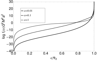
Figure 1: Energy part of the distribution function for a Plummer stellar sphere of scale $a$ embedded in a Hernquist dark matter halo of mass $M$ and scale $b$, and with constant velocity anisotropy $\beta=-1/2$, as given by Eq. (7). The various lines correspond to different degrees of embedding $\alpha=a/b$ of the stars in the (same) dark matter halo, $\alpha=0.01$ (solid), $0.1$ (dashed) and 1 (dotted).

We have checked that the density profile obtained by integrating this distribution function over velocity space returns the Plummer functional form. The left column of Fig. 2 shows the velocity dispersion profiles in the radial (solid) and tangential (dashed) directions for different values of $\alpha$, and makes explicit the dependence of the internal kinematics on the degree of embedding of the stars in the dark halo. For small $\alpha$ (top and middle left panels) the velocity dispersion profile is relatively flat for $r>0.1r/a$. Since the properties of the halo are fixed by the mass $M$ and the scale $b$, we note that the velocity dispersion has a smaller amplitude for smaller values of $\alpha$, as expected.

Figure 2: Velocity dispersion profiles associated to the distribution functions presented in Fig. 1 for different degrees of embedding, namely $\alpha=0.01,0.1$ and 1 from top to bottom. Left column: Intrinsic radial (solid) and tangential (dashed) velocity dispersions as function of radial distance $r/a$. Right column: Corresponding line-of-sight velocity dispersions as function of projected distance $R/a$. The resulting $\sigma_{\rm los}$ profiles are relatively flat, especially for small $\alpha$, i.e. 0.01 and 0.1, and reach a finite value at the centre. In general, the curves bare a good resemblance to the observed velocity dispersion profiles of stars in dSph satellites of the Milky Way, as determined in e.g. Walker et al. (2009).

In the right column of Fig. 2 we have plotted the resulting l.o.s. velocity dispersion profiles for the different values of $\alpha$ explored. It shows that these profiles are relatively flat with projected radius over the range $0<R/a<2$, which is similar to that probed by the observations the kinematics of stars in the dSph satellites of the Milky Way. If we set $M=10^{9}\text{M}_{\odot}$ and $b=2.5$ kpc, then the system with $\alpha=0.01$ (top panels) would have a velocity dispersion of $\sim 2$ km/s and $a\sim 25$ pc. On the other hand, if $\alpha=0.1$ (middle panels), then $a=250$ pc, and $\sigma_{\rm los}\sim 6.3$ km/s at the centre. This case could for example, represent systems akin the Carina, Sextans or Ursa Minor dSph. A more massive halo would probably be required if the aim is to represent systems like Sculptor or Fornax, as this would allow a better matching to the central value of $\sigma_{\rm los}$.

3 Conclusions

By example, we have demonstrated that a massless Plummer stellar system embedded in a Hernquist dark matter halo constitutes a plausible physical configuration. We have explicitly derived the form of the distribution function for the case of a tangential anisotropy $\beta=-1/2$ and for different degrees of embedding of the stars, as quantified by the ratio of scalelengths parameter $\alpha=a/b$. This distribution function is positive for the values of $\alpha=0.01-1$ and also leads to a system that is stable to radial modes, as $\partial f/\partial\epsilon>0$. The line-of-sight velocity dispersion profiles characteristic of this family of distribution functions resemble those observed for dSph, and hence can be used to represent these systems. They satisfy the An & Evans (2009) theorem, namely that $\gamma_{0}>2\beta_{0}$, but clearly not the equality condition. We have also explored the $\beta=-1$ case, and also found an analytic physical solution, though this is more cumbersome mathematically and hence not presented here.

References

- An & Evans (2009) An, J. H. & Evans, N. W. 2009, ApJ, 701, 1500
- Baes & Dejonghe (2002) Baes, M. & Dejonghe, H. 2002, A&A, 393, 485
- Battaglia et al. (2013) Battaglia, G., Helmi, A., & Breddels, M. 2013, ArXiv e-prints
- Binney & Tremaine (2008) Binney, J. & Tremaine, S. 2008, Galactic Dynamics (Princeton University Press)
- Breddels & Helmi (2013) Breddels, M. A. & Helmi, A. 2013, ArXiv e-prints
- Breddels et al. (2012) Breddels, M. A., Helmi, A., van den Bosch, R. C. E., van de Ven, G., & Battaglia, G. 2012, ArXiv e-prints
- Ciotti & Morganti (2010) Ciotti, L. & Morganti, L. 2010, MNRAS, 408, 1070
- Evans et al. (2009) Evans, N. W., An, J., & Walker, M. G. 2009, MNRAS, 393, L50
- Hernquist (1990) Hernquist, L. 1990, ApJ, 356, 359
- Irwin & Hatzidimitriou (1995) Irwin, M. & Hatzidimitriou, D. 1995, MNRAS, 277, 1354
- Jardel & Gebhardt (2012) Jardel, J. R. & Gebhardt, K. 2012, ApJ, 746, 89
- Jardel et al. (2013) Jardel, J. R., Gebhardt, K., Fabricius, M. H., Drory, N., & Williams, M. J. 2013, ApJ, 763, 91
- Koch et al. (2007) Koch, A., Kleyna, J. T., Wilkinson, M. I., et al. 2007, AJ, 134, 566
- Łokas (2001) Łokas, E. L. 2001, MNRAS, 327, L21
- Łokas (2009) Łokas, E. L. 2009, MNRAS, 394, L102
- Navarro et al. (1996) Navarro, J. F., Frenk, C. S., & White, S. D. M. 1996, ApJ, 462, 563
- Richardson & Fairbairn (2013) Richardson, T. & Fairbairn, M. 2013, MNRAS, 432, 3361
- Stoehr et al. (2002) Stoehr, F., White, S. D. M., Tormen, G., & Springel, V. 2002, MNRAS, 335, L84
- Strigari et al. (2010) Strigari, L. E., Frenk, C. S., & White, S. D. M. 2010, MNRAS, 408, 2364
- Walker (2012) Walker, M. G. 2012, arXiv:1205.0311
- Walker et al. (2007) Walker, M. G., Mateo, M., Olszewski, E. W., et al. 2007, ApJ, 667, L53
- Walker et al. (2009) Walker, M. G., Mateo, M., Olszewski, E. W., et al. 2009, ApJ, 704, 1274
- Wilkinson et al. (2002) Wilkinson, M. I., Kleyna, J., Evans, N. W., & Gilmore, G. 2002, MNRAS, 330, 778