Dynamical compactification in Einstein-Gauss-Bonnet gravity from geometric frustration

Abstract

In this paper we study dynamical compactification in Einstein-Gauss-Bonnet gravity from arbitrary dimension for generic values of the coupling constants. We showed that, when the curvature of the extra dimensional space is negative, for any value of the spatial curvature of the four dimensional space-time one obtains a realistic behavior in which for asymptotic time both the volume of the extra dimension and expansion rate of the four dimensional space-time tend to a constant. Remarkably, this scenario appears within the open region of parameters space for which the theory does not admit any maximally symmetric $(4+D)$-dimensional solution, which gives to the dynamical compactification an interpretation as geometric frustration. In particular there is no need to fine-tune the coupling constants of the theory so that the present scenario does not violate “naturalness hypothesis”. Moreover we showed that with increase of the number of extra dimensions the stability properties of the solution are increased.

I Introduction

The idea that space-time may have more than four dimensions goes back to Kaluza and Klein KK1 ; KK2 ; KK3 . They introduced one extra space dimension in an attempt to unify gravity with the electromagnetic interaction. There of course arise the question of why this extra dimension is not visible to us. A simple explanation of this fact is to assume that the extra dimension is compactified to a very small circle. Kaluza-Klein theory can be extended to include also non-Abelian gauge fields using more extra dimensions.

Extra dimensions appear naturally in the context of string theories as well. An interesting feature is that the low energy sector of some string theories (see, for instance, the discussion in GastGarr ) is described by an Einstein-Gauss-Bonnet theory rather then General Relativity. Einstein-Gauss-Bonnet (EGB) theory is actually the simplest generalization of General Relativity (GR) to higher dimensions in the sense that it leads to second order differential equations in the metric even if the action contains higher powers of the curvature. In four dimensions the Gauss-Bonnet term does not affect the equations of motion as it is a boundary term. However in any space-time dimension higher than four its variation gives a non-trivial contribution to the equations of motion. Einstein-Gauss-Bonnet gravity is member of a larger family of higher curvature gravity theories: indeed in any higher odd dimension it is possible to add to the gravitational action another higher power curvature term (in five dimensions – quadratic, in seven – cubic, in nine – quartic and so on) in such a way that the resulting equations of motion remain of second order. This family of gravity theories is called Lovelock gravity Lovelock .

One peculiar feature of the Einstein-Gauss-Bonnet theory, which distinguish it from standard General Relativity, is that the field equations do not necessarily imply the vanishing of torsion TZ-CQG , so that in the first order formalism, besides the graviton, there are additional propagating degrees of freedom related to the torsion. Indeed exact solutions with non-trivial torsion have been found CGT07 ; CGW07 ; CG ; CG2 ; ACGO , but here we will consider the torsion free case.

The most generic Einstein-Gauss-Bonnet action in any space-time dimension higher than four is the sum of three terms namely an Einstein-Hilbert term $\int\sqrt{-g}R$, a Gauss-Bonnet term $\int\sqrt{-g}(R_{\alpha\beta\mu\nu}R^{\alpha\beta\mu\nu}-4R_{\mu\nu}R^{\mu\nu}+R^{2})$ and a volume term $\int\sqrt{-g}\Lambda$. The volume term in the context of General Relativity is called the “cosmological term” however, as we will see in the next section, in the presence of a Gauss-Bonnet term, the value of the effective cosmological constant is actually a function of all three coupling constants and not just of the volume term. Indeed this theory being quadratic in the curvature can have up to two different maximally symmetric constant curvature solutions. The values of the curvature of the maximally symmetric solutions are the effective cosmological constants of the theory. Interestingly enough it can also happen for certain regions of the parameter space that the theory does not admit any maximally symmetric solution. This sector of the theory has not been studied very much up to now especially in the context of cosmology but it is actually of great theoretical interest since it generates in a natural way a symmetry breaking mechanism induced by geometry in which there is no solution with the maximum number of Killing fields which are allowed in principle by the geometry. In this sense one could speak of “geometric frustration”.

In cosmology the addition of Gauss-Bonnet term to the action is of special interest in order to study how it affects the size evolution of the extra dimensions (see add_1 ; add_2 ; add_3 ; add_4 ; add_5 ; add_6 ; add_7 ; add_8 ; add_9 ; add_10 ; add13 ; add_11 ; add_12 ; mpla09 ; prd09 ; grg10 ; gc10 ; prd10 ; new12 ; Germani:2002pt ; Kofinas:2003rz ; Papantonopoulos:2004jd ; 44 ; BD85 ; Is86 ; MO04 for older and recent developments in cosmology with Gauss-Bonnet and more general Lovelock terms; for an updated review and references see 1.5 ). In the context of extra dimensions the most important question is why the extra dimensions are small and of approximately constant size while the three space dimensions are much larger and expanding. The extra dimensions may have been much larger in the far past and non-constant in size. It is therefore of great interest to find a dynamical mechanism of compactification dictated just by the equations of motion derived from the gravitational action. A sensible requirement is that such a mechanism should not involve any fine-tuning of the coupling constants of the theory. Indeed, if the compactification mechanism only works for a precise value of the couplings of the theory, any small change could destroy it. Moreover in cosmology “naturalness” is often advocated, namely good phenomenological behavior should be obtained without assuming that one of the couplings of the theory is much smaller than the others. Such a dynamical mechanics was proposed in add13 for (5+1)-dimensional EGB theory; but we are proposing here a more generic setup with arbitrary number of extra dimensions, curvature in both manifolds and a volume term (Lambda term) in the action which opens new scenarios.

In CGTW , it was shown for the first time how to construct a realistic static compactification (namely, the extra dimensions do not evolve in time) in seven (or higher) dimensions in Lovelock gravities. A suitable class of cubic Lovelock theories allows to recover General Relativity with a small cosmological constant in four dimensions with the extra dimensions of constant curvature. However, in the cases analyzed in CGTW , in order to get the desired compactification both a fine-tuning (namely, one of the couplings is a function of the others) and a violation of “naturalness” are necessary. Here we want to improve such situation in a cosmological context within the framework of Einstein-Gauss-Bonnet theory.

We will therefore use the ansatz of a space-time which is a warped product of the form $M_{4}\times b(t)M_{D}$, where $M_{4}$ is a Friedmann-Robertson-Walker manifold with scale factor $a(t)$ whereas $M_{D}$ is a D-dimensional Euclidean compact and constant curvature manifold with scale factor $b(t)$ and study the evolution of the two scale factors. Due to the highly nonlinear nature of the equations of motion it is not possible to integrate them in a closed form. However it is possible to understand in detail all the relevant features of the theory depending on the values of the couplings and of the curvature of space and extra dimension by performing a numerical analysis.

In most cases, when considering the Gauss-Bonnet, or even higher-order Lovelock gravity, in literature spatially flat sections are considered. In our paper we decided to consider also the case with non-zero constant curvature as it allows us to see the influence of the curvature on the cosmological dynamics. Despite the fact that, according to current observational cosmological data, our Universe is flat with a high precision, at the early stages of the Universe evolution the curvature could comes into play. In there, negative curvature only “helps” inflation (since the effective equation of state for negative curvature is $w=-1/3$), while the positive curvature affects the inflationary asymptotics, but its influence is not strong for a wide variety of the scalar field potentials (see infl1 ; infl2 for details), so that we can safely consider both signs for curvature without worrying for inflationary asymptotics.

The structure of the paper is the following: in the second section we will give a basic review on the relevant features of Einstein-Gauss-Bonnet theory especially the relation between the couplings of the theory and the effective cosmological and Newton constant. In the third section we will write down the equations of motion for our metric ansatz in generic dimension and for generic space and extra dimension curvature. Later in the same section we will present the results, as well as discuss the stability of the solution in the large number of extra dimensions. In the last section the conclusions will be drawn.

II The Einstein-Gauss-Bonnet in arbitrary dimension

The Einstein-Gauss-Bonnet action in arbitrary dimension possesses 3 coupling constants and in the vielbein formalism reads

$$S=\int\epsilon_{{A_{1}}\ldots A_{D+4}}(\frac{c_{0}}{D+4}e^{A_{1}}\ldots e^{A_{D+4}}+\frac{c_{1}}{D+2}R^{{A_{1}}{A_{2}}}e^{A_{3}}\ldots e^{A_{D+4}}+\frac{c_{2}}{D}R^{A_{1}A_{2}}R^{A_{3}A_{4}}e^{A_{5}}\ldots e^{A_{D+4}})$$ (1)

The couplings $c_{2}$, $c_{1}$ and $c_{0}$ correspond the the Gauss-Bonnet term, Einstein-Hilbert term and the volume “cosmological” term respectively. When the Gauss-Bonnet coupling $c_{2}$ is zero the coupling $c_{0}$ is just the “cosmological constant” and the coupling $c_{1}$ is just be the Newton constant. However if $c_{2}$ is non-vanishing this is in general not true. Indeed the cosmological constant is the quantity which gives the curvature of the maximally symmetric solution of the theory. It is therefore useful to study the equations of motion obtained by varying the action with respect to the vielbein (which in the metric formalism correspond to the Einstein-Gauss-Bonnet field equations), they read

$$\epsilon_{A_{1}}=\epsilon_{{A_{1}}\ldots A_{D+4}}({c_{0}}e^{A_{2}}\ldots e^{A_{D+4}}+{c_{1}}R^{{A_{2}}{A_{3}}}e^{A_{4}}\ldots e^{A_{D+4}}+{c_{2}}R^{A_{2}A_{3}}R^{A_{4}A_{5}}e^{A_{6}}\ldots e^{A_{D+4}}).$$ (2)

The value of the $(4+D)$-dimensional “cosmological constant” is given by the value of the constant curvature of the maximally symmetric space-time solutions. The ansatz for a constant curvature space-time in the vielbein formalism reads

$$R^{AB}=\Lambda_{D+4}e^{A}e^{B},$$ (3)

where of course $\Lambda_{D+4}$ must be real. Plugging this ansatz into the equations of motion one gets a polynomial in $\Lambda_{D+4}$

$$(c_{2}\Lambda_{D+4}^{2}+c_{1}\Lambda_{D+4}+c_{0})e^{A_{1}}\ldots e^{A_{D+4}}=0;$$ (4)

this equation admits as solution

$$\Lambda_{eff}\equiv\Lambda_{D+4}=\frac{-c_{1}\pm\sqrt{(c_{1})^{2}-4c_{2}c_{0}}}{2c_{2}}.$$ (5)

This implies that in general the cosmological constant is a function of all three couplings of the action and not just $c_{0}$. If the discriminant is positive, the theory possesses two different possible cosmological constants which can even have opposite sign. A special case exists when the couplings are fine tuned in such a way that the discriminant is zero then the two roots of the polynomial are degenerate. In the case that $c_{0}\neq 0$ the discriminant can also be negative. In this case the two possible values for the cosmological constant are complex which means that in this case no maximally symmetric solution exists at all. This interesting phenomenon can be interpreted as induced by “geometric frustration” which prevents the existence of metrics preserving all the symmetries which in principle are available. It is worth noting that this can only happen when the highest power in the curvature of the Lovelock action is even (otherwise at least one real root would always exist). Moreover, the parameters region in which (at least) a maximally symmetric vacuum exist has been already extensively analyzed in the literature. Since it is known that, in such a region, it is not possible to obtain a dynamical compactification which is both free of fine-tunings and free of violations of the naturalness hypothesis, we will focus on the region in which geometric frustration occurs.

Another important feature of this theory, in opposition to GR, is that by compactifying the space-time to $M_{4}\times M_{D}$ where $M_{4}$ is a four dimensional space-time and $M_{D}$ is some compact manifold with constant curvature $\Lambda_{D}$ is that the Newton constant of the effective four dimensional theory is not just proportional to $c_{1}$. This can be seen by projecting the $4+D$ dimensional equations down to four dimensions

$$\begin{array}[]{l}\epsilon_{i}=\left(c_{1}(D+1)+2c_{2}(D-1)\Lambda_{D}\right)R^{jk}+\left(c_{0}\frac{(D+3)(D+2)(D+1)}{6}+\right.\\ \left.+c_{1}\Lambda_{D}\frac{(D+1)D(D-1)}{6}+c_{2}\Lambda_{D}^{2}\frac{(D-1)(D-2)(D-3)}{6}\right)e^{i}e^{j}=0.\end{array}$$ (6)

where the lowercase indices run from zero to three. The term $(c_{1}(D+1)+2c_{2}(D-1)\Lambda_{D})$ which multiplies the four dimensional curvature two form $R^{jk}$ is the “effective Newton constant” whereas the term $(c_{0}\frac{(D+3)(D+2)(D+1)}{6}+c_{1}\Lambda_{D}\frac{(D+1)D(D-1)}{6}+c_{2}\Lambda_{D}^{2}\frac{(D-1)(D-2)(D-3)}{6})$ is an “effective 4-dimensional cosmological constant”. This means that if the Gauss-Bonnet term does not vanish and moreover the $D$-dimensional curvature does not vanish the effective Newton constant is not just proportional to $c_{1}$. In particular, the effective Newton constant can even have a negative sign.

III Dynamical compactification

Nowadays it is widely accepted that the search for a unified theory requires additional space-time dimensions, the EGB theory being the simplest generalization of General Relativity to higher dimensions.

In the present paper we want to show that in a cosmological context one can get a dynamical compactification in an open region of the parameter space (and in agreement with the “naturalness hypothesis”) in which a potentially $4+D$ universe evolves towards a $4\times D$ universe in which the size of the extra dimensions is much smaller than the size of the 4 macroscopic dimensions. The key feature of EGB theory which gives rise to a phenomenologically realistic dynamical compactification is the possibility of geometric symmetry breaking mentioned above which can only occur in Lovelock theories in which the highest power of the curvature tensor is even.

The ansatz for the metric is

$$ds^{2}=-dt^{2}+a(t)^{2}d\Sigma_{(3)}^{2}+b(t)^{2}d\Sigma_{(\mathbf{D})}^{2}\ ,$$ (7)

where $d\Sigma_{(3)}^{2}$ and $d\Sigma_{(\mathbf{D})}^{2}$ stand for the metric of two constant curvature manifolds $\Sigma_{(3)}$ and $\Sigma_{(\mathbf{D})}$. It is worth to point out that even a negative constant curvature space can be compactified by making the quotient of the space by a freely acting discrete subgroup of $O(D,1)$ wolf . The vielbein can then be chosen as

$$e^{0}=dt;\;\;\;e^{i}=a(t)\tilde{e}^{i};\;\;\;e^{a}=b(t)\tilde{e}^{a},$$ (8)

where $\tilde{e}^{i}$ stands for the intrinsic vielbein of $\Sigma_{(3)}$, $\tilde{e}^{a}$ stands for the intrinsic vielbein of $\Sigma_{(\mathbf{D})}^{2}$, and $\epsilon^{ijk}$ is the Levi-Civita symbols on $\Sigma_{(3)}$.

The spin connection reads

$$\omega_{\ 0}^{i} = \frac{\overset{.}{a}}{a}e^{i};\;\;\;\omega_{\ 0}^{a}=\frac{\overset{.}{b}}{b}e^{a};\;\;\;\omega^{ij}=\tilde{\omega}^{ij},$$

$$\omega^{ab} = \tilde{\omega}^{ab};\ \ \omega^{jb}=0$$ (9)

where $\tilde{\omega}^{ij}$ corresponds to the intrinsic Levi-Civita connection of $\Sigma_{(3)}$, $\tilde{\omega}^{ab}$ corresponds to the intrinsic Levi-Civita connection of $\Sigma_{(\mathbf{D})}$.

The Riemannian curvature reads

$$R^{0i}=\frac{\overset{..}{a}}{a}e^{0}e^{i}\;;\;\;\;R^{0a}=\frac{\overset{..}{b}}{b}e^{0}e^{a};\ \ \ \ R^{ia}=\frac{\overset{.}{a}}{a}\frac{\overset{.}{b}}{b}e^{i}e^{a}$$

$$R^{ij}=\tilde{R}^{ij}+\left(\frac{\overset{.}{a}}{a}\right)^{2}e^{i}e^{j}\;;\;\;\;R^{ab}=\tilde{R}^{ab}+\left(\frac{\overset{.}{b}}{b}\right)^{2}e^{a}e^{b}$$ (10)

where $\tilde{R}^{ij}$ stands for the intrinsic Riemannian curvature of the manifold $\Sigma_{(3)}$, $\tilde{R}^{ab}$ stands for the intrinsic Riemannian curvature of the manifold $\Sigma_{(\mathbf{D})}$ (which will play the role of the extra-dimensional manifold). We will assume (as it is usual in literature) that $\Sigma_{(3)}$ and $\Sigma_{(\mathbf{D})}$ have constant Riemmanian curvatures given by $\gamma_{\left(3\right)}$ and $\gamma_{\left(\mathbf{D}\right)}$. It follows that

$$\tilde{R}^{ij} = \gamma_{\left(3\right)}\tilde{e}^{i}\tilde{e}^{j};\ \ \ \ \ \ \;\;\tilde{R}^{ab}=\gamma_{\left(\mathbf{D}\right)}\tilde{e}^{a}\tilde{e}^{b}$$

$$R^{ij} = \frac{\left[\gamma_{\left(3\right)}+\left(\overset{.}{a}\right)^{2}\right]}{a^{2}}e^{i}e^{j};\;\;\;\;\;\;R^{ab}=\frac{\left[\gamma_{\left(\mathbf{D}\right)}+\left(\overset{.}{b}\right)^{2}\right]}{b^{2}}e^{a}e^{b}$$

It will be convenient to use the following notation

$$R^{0i}=A_{(1)}e^{0}e^{i}\;\;\;;\;\;\;R^{0a}=B_{(1)}e^{0}e^{a}\;;\;\;\;R^{ia}=\mathring{R}^{ia}=Ce^{i}e^{a}\ ,$$ (11)

$$R^{ij}=A_{(2)}e^{i}e^{j},\ \ R^{ab}=B_{(2)}e^{a}e^{b}\ ,$$ (12)

with

$$A_{(1)} = \frac{\overset{..}{a}}{a},\ \ \ C=\frac{\overset{.}{a}\overset{.}{b}}{ab},\ \ \ B_{(1)}=\frac{\overset{..}{b}}{b},$$

$$A_{(2)} = \frac{\left[\gamma_{\left(3\right)}+\left(\overset{.}{a}\right)^{2}\right]}{a^{2}},\ \ \ B_{(2)}=\frac{\left[\gamma_{\left(\mathbf{D}\right)}+\left(\overset{.}{b}\right)^{2}\right]}{b^{2}}.$$ (13)

It will be convenient to define the following rescaled coupling constants appearing in the original action in (1)

$$\alpha=\frac{\left(D+3\right)\left(D+2\right)\left(D+1\right)}{6}c_{0}\ ,\ \ \ \beta=\frac{\left(D+1\right)D\left(D-1\right)}{6}c_{1}\ ,\ \ \ \gamma=\frac{\left(D-1\right)\left(D-2\right)\left(D-3\right)}{6}c_{2}\ .$$ (14)

Thus, $\beta$ is related to the coupling constant of the Einstein-Hilbert term, $\gamma$ corresponds to the Gauss-Bonnet coupling constant while $\alpha$ is a cosmological term. According to idea of “naturalness” discussed above, no one of the original coupling constants of the theory $c_{0}$, $c_{1}$ and $c_{2}$ is privileged with respect to the others: the three-dimensional parameters space of the theory will be analyzed without any fine-tuning.

The structure of the torsion-free equations of motions is the following:

$$\mathcal{E}_{A_{1}}=\left(c_{0}e^{A_{2}}\dots e^{A_{\mathbf{D}+4}}+c_{1}R^{A_{2}A_{3}}e^{A_{4}}\dots e^{A_{\mathbf{D}+4}}+c_{2}R^{A_{2}A_{3}}R^{A_{4}A_{5}}e^{A_{6}}\dots e^{A_{\mathbf{D}+4}}\right)\epsilon_{A_{1}A_{2}\dots A_{\mathbf{D}+4}}=0$$ (15)

Thus, the equations $\mathcal{E}_{0}=0$ and $\mathcal{E}_{i}=0$ read:

$$\mathcal{E}_{0} = 0\Leftrightarrow 0=\alpha+\beta\left(B_{(2)}+\frac{6}{D-1}C+\frac{6}{D\left(D-1\right)}A_{(2)}\right)+\gamma\left(B_{(2)}^{2}+\frac{12A_{(2)}B_{(2)}}{\left(D-2\right)\left(D-3\right)}+\right.$$ (16)

$$\left.+\frac{24C^{2}}{\left(D-2\right)\left(D-3\right)}+\frac{12B_{(2)}C}{\left(D-3\right)}+\frac{24A_{(2)}C}{\left(D-1\right)\left(D-2\right)\left(D-3\right)}\right),$$

$$\mathcal{E}_{i}=0\Leftrightarrow 0=\alpha+\beta\left(B_{(2)}+\frac{4A_{(1)}}{D\left(D-1\right)}+\frac{2B_{(1)}}{D-1}+\frac{2A_{(2)}}{D\left(D-1\right)}+\frac{4C}{\left(D-1\right)}\right)+\gamma\left(B_{(2)}^{2}+\right.$$

$$+\frac{16A_{(1)}C}{\left(D-1\right)\left(D-2\right)\left(D-3\right)}+\frac{8B_{(2)}C}{D-3}++\frac{8A_{(1)}B_{(2)}}{\left(D-2\right)\left(D-3\right)}+\frac{8A_{(2)}B_{(1)}}{\left(D-1\right)\left(D-2\right)\left(D-3\right)}+$$

$$\left.+\frac{16B_{(1)}C}{\left(D-2\right)\left(D-3\right)}+\frac{4B_{(1)}B_{(2)}}{\left(D-3\right)}+\frac{4A_{(2)}B_{(2)}}{\left(D-2\right)\left(D-3\right)}+\frac{8C^{2}}{\left(D-2\right)\left(D-3\right)}\right)\ \ ,$$ (17)

while the equation $\mathcal{E}_{a}=0$ reads

$$\mathcal{E}_{a}=0\Leftrightarrow 0=\frac{D}{\left(D-4\right)}\alpha+\frac{\left(D-2\right)}{\left(D-4\right)}\beta\left(B_{(2)}+\frac{6A_{(1)}}{\left(D-1\right)\left(D-2\right)}+\frac{2B_{(1)}}{D-2}+\frac{6A_{(2)}}{\left(D-1\right)\left(D-2\right)}+\frac{6C}{\left(D-2\right)}\right)+$$

$$+\gamma\left(B_{(2)}^{2}+\frac{48A_{(1)}C}{\left(D-2\right)\left(D-3\right)\left(D-4\right)}+\frac{12B_{(2)}C}{D-4}+\frac{24C^{2}}{\left(D-3\right)\left(D-4\right)}+\right.$$

$$+\frac{12A_{(1)}B_{(2)}}{\left(D-3\right)\left(D-4\right)}+\frac{24A_{(2)}B_{(1)}}{\left(D-2\right)\left(D-3\right)\left(D-4\right)}+\frac{24B_{(1)}C}{\left(D-3\right)\left(D-4\right)}+\frac{4B_{(1)}B_{(2)}}{\left(D-4\right)}+$$

$$\left.+\frac{12A_{(2)}B_{(2)}}{\left(D-3\right)\left(D-4\right)}+\frac{24A_{(2)}C}{\left(D-2\right)\left(D-3\right)\left(D-4\right)}+\frac{24A_{(1)}A_{(2)}}{\left(D-1\right)\left(D-2\right)\left(D-3\right)\left(D-4\right)}\right)$$ (18)

This notation in which the $D$ factors appear in the denominators is suitable for a large $D$ analysis in which one assumes that the physical quantities (the two scale factors in the present case) are analytic functions of $1/D$. Consequently, one can expand both scale factors in series of $1/D$ with time-dependent coefficients and replace the expressions into Eqs. (16), (17) and (18). This allows to derive a set of recursive equations order by order in the $1/D$ expansion. Although the expressions of the recursive equations become quite involved after few iterations, this provides one with a systematic way to compute $1/D$ corrections.

The cosmological equations are simply obtained by placing the expressions from (13) into Eqs. (16), (17) and (18). It is worth noting here that of the three equations (16), (17) and (18) only two are independent due to the Bianchi identities.

Thus, one has two evolution equations for the scale factors $a(t)$ and $b(t)$. Obviously, the ideal scenario is the one in which, without neither fine tunings nor violations of “naturalness”, one gets

$$\begin{array}[]{l}b(t)\underset{t\rightarrow\infty}{\rightarrow}b_{c}=\mathop{\rm const}\nolimits,\\ \frac{\dot{a(t)}}{a(t)}\underset{t\rightarrow\infty}{\rightarrow}H_{a}=\mathop{\rm const}\nolimits,\end{array}$$ (19)

since in this way the theory would approach for late time to an effective four dimensional universe with small compact extra dimensions.

We leave the complete description of all possible regimes and their abundance to a separate paper, here we state that this scenario is present in a case with negative discriminant of (4) (so that $\Lambda_{eff}$ (5) is imaginary) and negative curvature of the extra dimensions ($\gamma_{\left(\mathbf{D}\right)}=-1$ regardless of the $\gamma_{(3)}$).

To the best of authors knowledge this is the first time that a dynamical compactification in which the size of extra dimensions approaches to a constant while the three macroscopic extra dimensions expand has been achieved without fine tunings or ad hoc matter fields.

Finally, let us describe the region on the $\{c_{0},\,c_{1},\,c_{2}\}$ parameters space which satisfy both the condition for $\Lambda_{eff}$ to be imaginary and the condition for effective Newton constant $G_{N,\,eff}=c_{1}(D+1)+2c_{2}(D-1)\Lambda_{D}$ to be positive. So the system of inequalities is (we put $\Lambda_{D}=-1$ since only this choice gives us “well-behaved” regime)

$$\begin{array}[]{l}G_{N,\,eff}=c_{1}(D+1)-2c_{2}(D-1)>0,\\ c_{1}^{2}-4c_{0}c_{2}<0;\end{array}$$ (20)

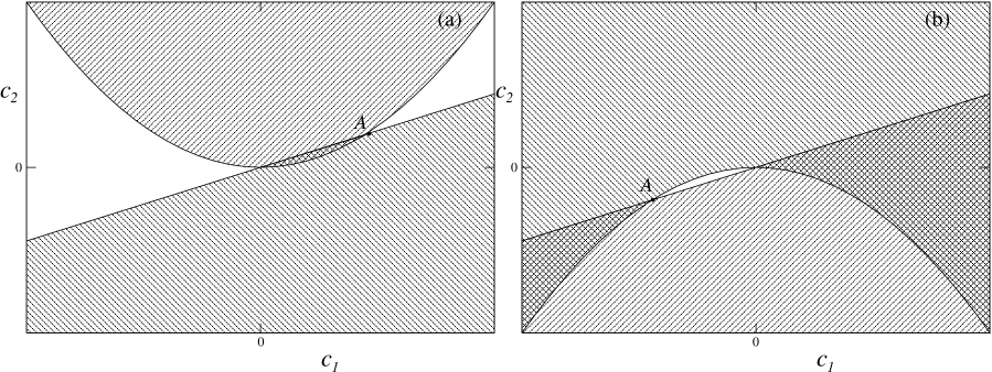
Figure 1: The area on the $(c_{1},\,c_{2})$ space which corresponds to the requirements of the positivity of the effective Newton constant and negativity of the discriminant of (4) is represented as double-dashed region. The (a) panel corresponds to the $c_{0}>0$ case while (b) panel – to the $c_{0}<0$ (see text for details).

we plot these two inequalities in the $(c_{1},\,c_{2})$ coordinates in Fig. 1. There we dashed with different inclinations each of (20) conditions so that double-dashed region corresponds to the case where both of them satisfied. In (a) panel we presented the data for $c_{0}>0$ case while in the (b) panel – for $c_{0}<0$. The coordinates for the $A$ point are: $c_{1}=2c_{0}(D+1)/(D-1)$, $c_{2}=c_{0}(D+1)^{2}/(D-1)^{2}$ – it is true for both panels since the sign for $c_{0}$ is different in them. So that one can see that in $c_{0}>0$ case the area for possible $(c_{1},\,c_{2})$ is compact while in $c_{0}<0$ it is noncompact. Let us note also that “classical value” for $c_{0}$ is $c_{0}=-2\Lambda$, where $\Lambda$ is “classical” cosmological constant, so that the negative value for $c_{0}$ is favored both by noncompactness of the corresponding region and by “classical argumentation”.

III.1 Late time behavior

In this subsection let us analyze the late-time behavior of the system. Here we apply the late-time asymptotic of the region which we are interested in ($b(t)=b_{c}$, $H(t)=H_{a}$). Before giving the equations themselves, let us note one thing – there are two main late-time regimes from the extra dimensions perspective – one with $b(t)=b_{0}$ and so $H_{b}\to 0$ and the other is $H_{b}>0$ and so $\gamma_{\left(\mathbf{D}\right)}+\dot{b}(t)^{2}\to H_{b}^{2}$. Obviously, the latter of them is just flat case, while former involves curvature. The same is true for $M_{4}$ as well – if we impose nonzero curvature on it, the only difference would be appearance of the regime with $a(t)=a_{c}=\mathop{\rm const}\nolimits$ with $H_{a}\to 0$, which obviously contradicts cosmological data. So, with $b(t)=b_{c}$, $H(t)=H_{a}$ ansatz, equations (16)–(18) take a form:

$$\begin{array}[]{l}\alpha+\beta y+\displaystyle\frac{6\beta x}{D(D-1)}+\gamma y^{2}+\displaystyle\frac{12\gamma xy}{(D-2)(D-3)}=0,\end{array}$$ (21)

$$\begin{array}[]{l}\alpha D+\beta(D-2)y+\displaystyle\frac{12\beta x}{D-1}+\gamma(D-4)y^{2}+\displaystyle\frac{24\gamma xy}{D-3}+\displaystyle\frac{24\gamma x^{2}}{(D-1)(D-2)(D-3)}=0,\end{array}$$ (22)

where we put $y=\gamma_{\left(\mathbf{D}\right)}/b_{c}^{2}$ and $x=H_{a}^{2}$. It appears that (21) corresponds to both $\mathcal{E}_{0}=0$ and $\mathcal{E}_{i}=0$ – rather, we have $\mathcal{E}_{i}=\mathcal{E}_{0}$ since there is no dynamics in extra dimensions; (22) corresponds to $\mathcal{E}_{a}=0$. System (21)–(22) could be further simplified to one fourth-order equation with respect to $y$, but cannot be generally solved. Numerically we verified that for wide range of $\{c_{0},c_{1},c_{2}\}$ that gives imaginary $\Lambda_{eff}$ there are solutions of (21)–(22) with $x>0$ (it must holds since $x=H_{0}^{2}$) and only $y<0$, which gives $\gamma_{\left(\mathbf{D}\right)}=-1$.

III.2 Stability of the solution

In this subsection we want to check the stability of the solution $b(t)=b_{c}$, $H(t)=H_{a}$. So we perturbed it as $b(t)=b_{c}+\delta b$, $H(t)=H_{a}+\delta H$, and substitute them into (16)–(18). The resulting system could be brought to one second-order equation with respect to $\delta b$:

$$\begin{array}[]{l}a_{2}\delta\ddot{b}+a_{1}\delta\dot{b}+a_{0}\delta b=0,\end{array}$$ (23)

where $a_{i}=a_{i}(c_{0},c_{1},c_{2},D,\gamma_{\left(\mathbf{D}\right)})$ are very nasty polynomial coefficients. Due to the nature of the coefficients, it is almost impossible to study them analytically, so we solved (23) numerically. Our numerical study revealed that the solution is stable for a wide range of the parameters and the initial conditions which lead the $b(t)=b_{c}$, $H(t)=H_{a}$ solution.

But in the large $D$ limit (23) behave in a interesting way: we have $\{a_{2},\,a_{1}\}\propto D^{5}$ while $a_{0}\propto D^{6}$ which implies that with increase of $D$ the solution becomes more stable. One can make a mechanical analogy with excitation of a massive string – increasing mass of the string makes it more difficult to excite it. The large $D$ limit General Relativity in the context of compactification has been also studied in CGZ ; Baskal ; Guendelman . The large $D$ limit in the context of Lovelock gravity has been studied in Giribet . In both cases it is manifest that the large $D$ limit improves the behavior of the theory. Here we have confirmed that in this limit the stability of the dynamical compactification regime improves as well.

IV Discussion and comments

In this paper it has been shown that EGB gravity gives rise to dynamical compactification in which an initially $4+D$ Universe evolves towards a $4\times D$ Universe in which the size of the extra dimensions are much smaller than the size of the non-compact ones. We have investigated numerically the system under consideration and found that a phenomenologically realistic scenario happens for open region of the couplings space $\{c_{0},\,c_{1},\,c_{2}\}$ where the theory does not admit a maximally symmetric vacuum solution. This scenario can therefore be interpreted as symmetry breaking mechanism.

Remarkably this scenario does not require neither fine-tunings nor violations of “naturalness hypothesis”. Independently of the sign of the curvature of the three dimensional space section the curvature of the extra dimensional space must be negative.

As we mentioned in the Introduction, the similar result – the dynamical compactification without violation of “naturaless” – was proposed in add13 for the (5+1)-dimensional EGB theory. As one can see, our setup is different from the one used in add13 – we considered both $M_{D}$ and $M_{4}$ as manifolds with constant and possibly nonzero curvature, which gives a rise to additional curvature terms and, as a consequence, to a new regime. Additionally, we considered all possible geometrical terms, including the boundary term ($c_{0}\neq 0$), which also affects the dynamics. Overall, despite the fact that in both cases – in add13 and in our paper – we can see dynamical compactification, it is brought by different phenomena. In our case it is geometric frustration, which is brought by a combination of nonzero curvature and nonzero boundary term – both of them are usually omitted from consideration since they complicate the equations a lot. But one can see that if you consider such thems, new beautiful regimes could appear; in that sence our paper holds some methodological character as well.

In the analysis of the dynamical compactification we have supposed the torsion to be zero. However in first order formalism the equations of motion of EGB gravity do not imply the vanishing of torsion which is therefore a propagating degree of freedom. To study its effects in the context of dynamical compactification will be object of future investigation.

EGB gravity is the simplest generalization of general relativity within the class of Lovelock gravity. As we considered an arbitrary number of extra dimensions it would also be interesting to study the effect of higher order Lovelock terms in the compactification mechanism. The results obtained in this paper suggest that the effects of higher terms depend sensibly on the fact if the highest curvature power is even as only in this case there exist a region in the parameter space admits no maximally symmetric solution.

Acknowledgments.– This work was supported by Fondecyt grants 1120352, 1110167, and 3130599. The Centro de Estudios Cientificos (CECs) is funded by the Chilean Government through the Centers of Excellence Base Financing Program of Conicyt. S.A.P. was partially supported by RFBR grant No. 11-02-00643.

References

- (1) T. Kaluza, Sit. Preuss. Akad. Wiss. K1, 966 (1921).
- (2) O. Klein, Z. Phys. 37, 895 (1926).
- (3) O. Klein, Nature 118, 516 (1926).
- (4) C. Garraffo and G. Giribet, Mod. Phys. Lett. A23, 1801 (2008).
- (5) D. Lovelock, J. Math. Phys. 12, 498 (1971).
- (6) R. Troncoso and J. Zanelli, Class. Quant. Grav. 17, 4451 (2000) [arXiv:hep-th/9907109].
- (7) F. Canfora, A. Giacomini, and R. Troncoso, Phys. Rev. D77, 024002 (2008).
- (8) F. Canfora, A. Giacomini, and S. Willison, Phys. Rev. D76, 044021 (2007).
- (9) F. Canfora and A. Giacomini, Phys. Rev. D78, 084034 (2008).
- (10) F. Canfora and A. Giacomini, Phys. Rev. D82, 024022 (2010).
- (11) A. Anabalon, F. Canfora, A. Giacomini, J. Oliva, Phys. Rev. D84, 084015 (2011).
- (12) M. Mezard, G. Parisi, M. Virasoro, Spin Glass Theory and Beyond, World Scientific (1987).
- (13) V. Dotsenko, Introduction to the Replica Theory of Disordered Statistical Systems, Cambridge University Press (2001).
- (14) F. Mller-Hoissen, Phys. Lett. 163B, 106 (1985).
- (15) J. Madore, Phys. Lett. 111A, 283 (1985).
- (16) J. Madore, Class. Quant. Grav. 3, 361 (1986).
- (17) F. Mller-Hoissen, Class. Quant. Grav. 3, 665 (1986).
- (18) N. Deruelle, Nucl. Phys. B327, 253 (1989).
- (19) T. Verwimp, Class. Quant. Grav. 6, 1655 (1989).
- (20) G. A. Mena Marugán, Phys. Rev. D 42, 2607 (1990).
- (21) G. A. Mena Marugán, Phys. Rev. D 46, 4340 (1992).
- (22) N. Deruelle and L. Faria-Busto, Phys. Rev. D 41, 3696 (1990).
- (23) J. Demaret, H. Caprasse, A. Moussiaux, P. Tombal, and D. Papadopoulos, Phys. Rev. D 41, 1163 (1990).
- (24) E. Elizalde, A.N. Makarenko, V.V. Obukhov, K.E. Osetrin, and A.E. Filippov, Phys. Lett. B644, 1 (2007).
- (25) M. Farhoudi, Gen. Rel. Grav. 41, 117 (2009).
- (26) A. Toporensky and P. Tretyakov, Gravitation & Cosmology 13, 207 (2007).
- (27) S.A. Pavluchenko and A.V. Toporensky, Mod. Phys. Lett. A24, 513 (2009).
- (28) S.A. Pavluchenko, Phys. Rev. D80, 107501 (2009).
- (29) I.V. Kirnos, A.N. Makarenko, S.A. Pavluchenko, and A.V. Toporensky, General Relativity and Gravitation 42, 2633 (2010).
- (30) I.V. Kirnos, S.A. Pavluchenko, and A.V. Toporensky, Gravitation & Cosmology 16, 274 (2010).
- (31) S.A. Pavluchenko, Phys. Rev. D82, 104021 (2010).
- (32) S.A. Pavluchenko and A.V. Toporensky, arXiv:1212.1386.
- (33) C. Germani and C. F. Sopuerta, Phys. Rev. Lett. 88, 231101 (2002) [arXiv:hep-th/0202060].
- (34) G. Kofinas, R. Maartens, and E. Papantonopoulos, JHEP 0310, 066 (2003) [arXiv:hep-th/0307138].
- (35) E. Papantonopoulos, arXiv:gr-qc/0402115.
- (36) J. Kripfganz and H. Perlt, Acta Phys. Polon. B 18, 997 (1987).
- (37) D. G. Boulware and S. Deser, Phys. Rev. Lett. 55, 2656 (1985).
- (38) H. Ishihara, Phys. Lett. B179, 217 (1986).
- (39) K.I. Maeda and N. Ohta, Phys. Rev. D71, 063520 (2005).
- (40) F. Ferrer and S. Rasanen, JHEP 0711, 003 (2007) [arXiv:0707.0499].
- (41) F. Canfora, A. Giacomini, R. Troncoso, and S. Willison, Phys. Rev. D80, 044029 (2009) [arXiv:0812.4311 [hep-th]].
- (42) S.A. Pavluchenko, Phys. Rev. D67, 103518 (2003).
- (43) S.A. Pavluchenko, Phys. Rev. D69, 021301 (2004).
- (44) J.A. Wolf, Spaces of constant curvature, 4th edition (Publish or Perish, Wilmington, Delaware USA, 1984), p. 69.
- (45) F. Canfora, A. Giacomini, and A. R. Zerwekh, Phys. Rev. D80, 084039 (2009).
- (46) S. Baskal and H. Kuyrukcu, Gen. Rel. Grav. 45, 359 (2013).
- (47) E. I. Guendelman, Class. Quant. Grav. 29, 105007 (2012).
- (48) G. Giribet, Phys. Rev. D87, 107504 (2013).