Executive Summary

We propose the construction of a compact Muon Collider $s$-channel Higgs Factory. A Muon Collider Higgs Factory is part of an evolutionary program beginning with R&D on Muon Cooling with a possible neutrino factory such as $\nu$STORM, the construction of Project-X with a rich program of precision physics addressing the $\sim 100~{}{\rm TeV}$ scale, potentially leading ultimately to the construction of an energy frontier Muon Collider with $\mu^{+}$ and $\mu^{-}$ colliding up to $\sim 10.0~{}{\rm TeV}$ center-of-mass energy. The Muon Collider Higgs Factory would utilize an intense proton beam from Project-X.

The Higgs boson is a particle of fundamental importance to physics. Measuring its properties with precision will allow us to probe the limits of the standard model, and may point toward non-standard model physics. Using simple estimates of physics backgrounds and separable signals, we have estimated that with $4.2~{}{\rm fb}^{-1}$ of integrated luminosity a Muon Collider Higgs Factory, directly producing the Higgs as an $s$-channel resonance, can determine the mass of the Higgs boson to a precision of $\pm 0.06~{}{\rm MeV}$, and its total width to $\pm 0.18~{}{\rm MeV}$. We estimate that, with a beam spread of $\sim 4.2~{}{\rm MeV}$, approximately $368{\rm~{}pb}^{-1}$ total integrated luminosity would be required to locate the narrow Higgs peak. We believe that these preliminary results strongly motivate further research and development towards the construction of a Muon Collider Higgs factory.

Our estimates plausibly assume there is managable machine-induced background and that the detector has excellent tracking and calorimetry. Our results underscore the value of the large, resonant Higgs cross section and narrow beam energy spread available at a muon collider. These two factors enable the direct measurement of the Higgs mass and width by scanning the Higgs s-channel resonance, which is not possible at any $e^{+}e^{-}$ collider. Our study of the physics-induced background and separation of the Higgs signal shows that significant reduction of the physics background can be achieved by a detector with high energy and spatial resolution. We believe that this justifies a more in-depth analysis of Higgs channels and their backgrounds, for example the reconstruction of $h\rightarrow WW^{*}\rightarrow 4j$ events using learning algorithms, or the application of flavor-tagging techniques to tag $b\overline{b}$ and $c\overline{c}$ events.

While there has been considerable progress in understanding machine-induced backgrounds, mainly from muon decays in the beam, these present a challenge which has not yet been studied in sufficient detail. We believe that, in addition to significant shielding in the detector cone and endcaps, it will be important to have a calorimeter with high spatial and temporal resolution. Our results motivate an in-depth analysis of the machine-induced background including simulation in a highly segmented, totally-active, dual readout calorimeter such as the MCDRCal01 detector concept.

A community letter supporting this project has been submitted previously to the archive [2].

Contents

1. 1 Introduction
2. 2 Physics at a Muon Collider Higgs Factory
   1. 2.1 Higgs Boson Signal and Background
   2. 2.2 Locating the Mass Window of the Higgs Boson
   3. 2.3 Precision Determination of the Total Width
3. 3 Collider Environment
   1. 3.1 Machine Performance and Environment
   2. 3.2 Energy Determination by Spin Tracking
   3. 3.3 Accelerator Backgrounds
4. 4 Detector Design
   1. 4.1 Tracking
   2. 4.2 Calorimetry
   3. 4.3 Software Environment
   4. 4.4 Background Rejection Techniques
5. 5 Detector Simulation Studies of Higgs Physics
   1. 5.1 Including Backgrounds
      1. 5.1.1 $h\rightarrow b\overline{b}$
      2. 5.1.2 $h\rightarrow WW^{*}$
      3. 5.1.3 $h\rightarrow\tau^{+}\tau^{-}$
      4. 5.1.4 $h\rightarrow c\overline{c}$
   2. 5.2 Combining Channels
   3. 5.3 Potential to Resolve Nearly Degenerate Higgs Bosons
   4. 5.4 Testing the CP Property

1 Introduction

The recent discovery of a particle with a mass of $126~{}{\rm GeV}$ [3] and with a favored $J^{PC}=0^{++}$ is widely interpreted as a Higgs boson, as anticipated by Weinberg in the original incarnation of the standard model [4]. The Higgs boson “accommodates” the masses of quarks, leptons and electroweak gauge bosons seen in nature. However, the origin of the Higgs-Yukawa coupling constants and mixing angles, as well as the origin of the Higgs boson mass itself, remain a mystery. The most important issues facing modern high energy physics are, therefore, to fully understand the origin of electroweak symmetry breaking and to probe for any associated new physics at the electroweak scale.

New physics can potentially be revealed in detailed studies of Higgs boson parameters, such as the mass, decay widths and production amplitudes. Indeed, the LHC will go a long way toward revealing these detailed properties. New physics may also be discovered at higher energy scales indirectly, e.g., through precision experiments at the “Intensity Frontier,” such as through rare kaon decays, electric dipole moment searches, and probes of charged lepton and neutrino flavor physics. This is the purpose of “Project-X” in the near term at Fermilab. However, it is also important that the field continues to evolve along the path toward the direct probes of new physics, i.e., at the “Energy Frontier.” This demands a cost effective, and upward scalable (in energy) strategy toward a program that can shed further light on the questions of electroweak physics and detailed properties of the Higgs boson.

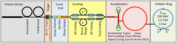
Figure 1: Muon Collider schematic. A Higgs factory is simpler since it does not use final cooling and does not use a RCS.

An attractive option along this path is the development of an $s$-channel Higgs factory using muons in a compact circular collider, i.e., a “Muon Collider Higgs Factory”[2, 5]. The muon has a Higgs-Yukawa coupling constant that enables direct $s$-channel production of the standard model Higgs boson at an appreciable rate. With an attainable, very small beam energy resolution of order $\sim 4~{}{\rm MeV}$ operating at an energy of $m_{h}/2=63$ GeV and at a nominal luminosity of about $\sim 10^{32}$ cm^-2 s^-1 such a collider would produce $17,000$ Higgs bosons per year. It affords precise observation of the mass and width of the Higgs boson by direct scanning, and the most precise determination of a Higgs-Yukawa coupling constant, that of the muon itself.

Table 1: Parameters of a $\mu^{+}\mu^{-}$ Collider at 126 GeV center-of-mass energy. The baseline design is shown.

Since the muon is about 200 times heavier than an electron, synchrotron radiation from muon beams in a small radius circular machine is dramatically suppressed. This allows a muon collider facility to be much smaller than an $e^{+}e^{-}$ facility at the same center-of-mass energy. The machine we are describing presently is detailed by Neuffer [6] and involves a collider storage ring of approximately $100$ meters in diameter, roughly the size of the Fermilab Booster. The Muon Collider also provides superb energy resolution and an attractive way to experimentally precisely measure the beam energy.

A conceptual design for a Muon Collider Higgs Factory facility is shown in Fig. 1, consisting of a source of short high-intensity proton pulses, a production target with collection of secondary $\pi$-mesons, followed by a decay channel. The produced $\mu^{\pm}$’s are collected and enter a bunching and cooling channel. Narrow intense muon pulses are then accelerated.

Using clever sequencing and timing, the separate $\mu^{-}$ and $\mu^{+}$ bunches can be accelerated in the Project-X linac that produces the original intense proton source, up to $\sim 0.5\times 10^{12}$ $\mu^{+}$ and $\mu^{-}$ bunches. For higher luminosities we require an extended linac of the same type used for Project X with recirculation arcs. The accelerated bunches are injected into the collider storage ring for collisions within an interaction region inside a detector.

The parameters for a Muon Collider Higgs Factory are given in Table 1 [7]. The lattice for the baseline design is shown in Fig. 2. With these parameters, luminosities of $1.7$ to $8.0$ $\times 10^{31}$ cm^-2s^-1 can be achieved, giving 3,400 to 13,600 Higgs bosons per year.

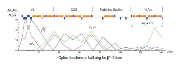
Figure 2: Muon Collider Higgs Factory lattice.

2 Physics at a Muon Collider Higgs Factory

A Muon Collider Higgs Factory has the following a priori advantages for physics:

• Small beam energy resolution (SBER) $\delta E/E\mathrel{\vbox{\hbox{$<$}\nointerlineskip\hbox{$\sim$}}}\makebox{(few)}\times 10^{-5}$, allowing the study of direct s-channel production and a line-shape scan of the Higgs boson, as well as other heavier Higgs bosons as in multi-Higgs models.

• The s-channel Higgs production affords the most precise measurement of a second generation fermion Higgs-Yukawa coupling constant, the muon coupling, $g_{\mu}$, to a precision $\delta g_{\mu}/g_{\mu}\sim\makebox{(few)}\%$. It allows the measurement of the renormalization group running of $g_{\mu}(q^{2})$ from $q^{2}=0$ to $q^{2}=m_{h}^{2}$ [8].

• The s-channel Higgs production affords the best mass measurement of the Higgs boson to a precision of $\sim\makebox{(few)}\times 10^{-6}$ with a luminosity of ${\cal{L}}\sim 10^{32}$ cm^-2s^-1.

• It affords the best direct measurement of the Higgs boson width to a precision of $\sim\makebox{few}$% with a luminosity of ${\cal{L}}\sim 10^{32}$ cm^-2s^-1; see Tables [2] and [3] below.

• This would yield the most precise measurement of Higgs branching ratios to $WW^{*}$, $ZZ^{*}$ and $b\overline{b}$.

• At an upgraded luminosity of ${\cal{L}}\sim 10^{33}$ cm^-2s^-1 and $\sim 3$ “snowmass years” on the Z-pole, we would produce $\sim 10^{9}$, Z-bosons; thus the Muon Collider Higgs Factory upgrade permits a “Giga-Z program.”

Detailed studies of these and other issues are underway, including: (1) optimal search strategy for the Higgs peak establishing a threshold integrated luminosity for physics of about $\sim\makebox{(few)}\times 10^{31}$ cm^-2s^-1 [11, 12] ; (2) charm decay mode $h\rightarrow c\overline{c}$ appears to be accessible at a level of $\sim 8\sigma$ [13] ; (3) possible observable interference effects may occur in e.g., $h\rightarrow WW^{*}$; (4) the mode $h\rightarrow Z\gamma^{*}\rightarrow Z\ell\ell$ may prove to be an interesting mode for study the decay spectrum.

In Section (5) we will discuss the physics and detector issues for many standard Higgs boson processes. We turn presently to a brief discussion of the location and line-shape scan of the Higgs boson, produced directly in the $s$-channel, at a Muon Collider Higgs Factory.

2.1 Higgs Boson Signal and Background

One of the most appealing features of a muon collider Higgs factory is its $s$-channel resonant production of Higgs bosons. For the production $\mu^{+}\mu^{-}\to h$ and a subsequent decay to a final state $X$ with a $\mu^{+}\mu^{-}$ (partonic) c.m. energy $\sqrt{\hat{s}}$, the Breit-Wigner resonance formula is:

$$\sigma(\mu^{+}\mu^{-}\to h\to X)=\frac{4\pi\Gamma_{h}^{2}\,{\rm Br}(h\to\mu^{+}\mu^{-})\,{\rm Br}(h\to X)}{(\hat{s}-m^{2}_{h})^{2}+\Gamma_{h}^{2}m_{h}^{2}},$$ (2.1)

At a given energy, the cross section is governed by three parameters: $m_{h}$ for the signal peak position, $\Gamma_{h}$ for the line shape profile, and the product $B\equiv{\,{\rm Br}}(h\to\mu^{+}\mu^{-}){\,{\rm Br}}(h\to X)$ for the overall event rate.

In reality, the observable cross section is given by the convolution of the energy distribution delivered by the collider with eq(2.1). Assuming that the $\mu^{+}\mu^{-}$ collider c.m. energy ($\sqrt{s}$) has a luminosity distribution

$${dL(\sqrt{s})\over d\sqrt{\hat{s}}}={\frac{1}{\sqrt{2\pi\Delta}}}\exp[\frac{-(\sqrt{\hat{s}}-\sqrt{s})^{2}}{2\Delta^{2}}],$$

with a Gaussian energy spread $\Delta=R\sqrt{s}/\sqrt{2}$, where $R$ is the relative beam energy resolution, then the effective cross section is

$$\sigma_{\rm eff}(s)=\int d\sqrt{\hat{s}}\ \frac{dL(\sqrt{s})}{d\sqrt{\hat{s}}}\sigma(\mu^{+}\mu^{-}\to h\to X)$$ (2.2)

The excellent beam energy resolution of a muon collider allows a direct determination of the Higgs boson width, in contrast to the situations in the LHC and ILC [6]. We calculate the effective cross sections at the peak for two different energy resolutions, $R=0.01\%$ and $R=0.003\%$. We further evaluate the signal and SM background for the leading channels, $h\to b\overline{b},~{}WW^{*}$.

We impose a polar angle acceptance for the final-state particles, $10^{\circ}<\theta<170^{\circ}$. We assume a $60\%$ single $b$-tagging efficiency and require at least one tagged $b$ jet for the $b\overline{b}$ final state. The backgrounds are assumed to be flat with cross sections evaluated at $126~{}~{}{\rm GeV}$ using Madgraph5 [9].

	$\mu^{+}\mu^{-}\rightarrow h$	$h\rightarrow b\overline{b}$		$h\rightarrow WW^{*}$
R (%)	$\sigma_{\rm eff}$ (pb)	$\sigma_{Sig}$	$\sigma_{Bkg}$	$\sigma_{Sig}$	$\sigma_{Bkg}$
$0.01$	$16$	$7.6$		$3.7$
$0.003$	$38$	$18$	$15$	$5.5$	$0.051$

Table 2: Effective cross sections (in pb) at the resonance $\sqrt{s}=m_{h}$ for two choices of beam energy resolutions $R$ and two leading decay channels, with the SM Higgs branching fractions $\,{\rm Br}_{b\overline{b}}=56\%$ and $\,{\rm Br}_{WW^{*}}=23\%$ [Dittmaier:2012vm]. This table is taken from Ref [10].

Results are tabulated in Table 2. The background rate of $\mu^{+}\mu^{-}\rightarrow Z^{*}/\gamma^{*}\to b\overline{b}$ is $15~{}\,{\rm pb}$, and the rate of $\mu^{+}\mu^{-}\to WW^{*}\to 4$ fermions is only $51~{}\,{\rm fb}$, as shown in Table 2. Here we consider all decay modes of $WW^{*}$ because of its clear signature at a muon collider. The four-fermion backgrounds from $Z\gamma^{*}$ and $\gamma^{*}\gamma^{*}$ are initially smaller, but can be greatly reduced by kinematical constraints, such as requiring the invariant mass of one pair of jets to be near $m_{W}$ and setting a lower cut on the invariant mass of the other pair.

2.2 Locating the Mass Window of the Higgs Boson

The first challenge at the muon collider is to locate the Higgs boson mass within a fine mass window. The theoretical natural width of a $125~{}{\rm GeV}$ Higgs is $4.07~{}{\rm MeV}$. It is expected that the Higgs mass will be known to better than $\sim 100~{}{\rm MeV}$ from measurements at the LHC. After the Higgs has been located, the Muon Collider can be used to scan the line-shape and then tuned to sit on the peak of the Higgs resonance to study Higgs physics.

A. Conway, H. Wenzel [11] and E. Eichten [12] have developed the optimal strategy to locate the Higgs boson at a Muon Collider. The required total luminosity is determined to observe a $5\sigma$ ($3\sigma$) Higgs boson signal with various likelihoods and energy steps. It was assumed that a center-of-mass energy resolution of $3.54$ MeV is obtainable at a Muon Collider.

Two decay channels were considered: (1) the $b\overline{b}$ final state and (2) the $WW^{*}$ final state. The $b\overline{b}$ final state has the largest branching fraction, but has a significant background, even with the excellent energy spread possible at the muon collider. The $WW^{*}$ channel has very small background physics rates (two orders of magnitude smaller than the Higgs signal). For this study the $WW^{*}$ decays with one neutrino-lepton pair are used.

The best strategy was found to use energy steps equal to the beam energy spread with the choice of the next energy bin determined by the maximum probability of discovery weighted by the prior of the LHC measurements. The $WW^{*}$ channel is the most effective but both channels are included in the final results. The results for the combined channels from Conway and Wenzel [11] is shown in Table 3 for various p-values of non-discovery.

Channel	$\sigma_{sig}\ (pb)$	Luminosity Required $(pb^{-1})$
	$\sigma_{bkgr}\ (pb)$	$3\sigma$ signal	$5\sigma$ signal
$b\overline{b}$ (Cut)	$\sigma_{s}=4.0$	1,100	2,200
	$\sigma_{b}=6.3$
$WW^{*}$ (Cut)	$\sigma_{s}=1.9$	400	1,100
	$\sigma_{b}=0.001$
$b\overline{b},\ WW^{*}$	$\sigma_{s}=--$	600	900
	$\sigma_{b}=--$

Table 3: Required luminosity to guarantee finding a $3$ or $5\sigma$ Higgs signal with confidence level $p=3\sigma$ [11].

It is clear from Table 3 that reducing the error on the LHC determination of the mass of the Higgs could greatly aid finding the Higgs resonance at a Muon Collider.

2.3 Precision Determination of the Total Width

The total decay width ($\Gamma_{h}$) is one of the most important of all of the Higgs boson properties. Once the total width is known, the measurement of the partial decay widths to different channels yields model-independent determination of Higgs boson coupling strengths.

We first generate pseudo-data in accordance with a Breit-Wigner resonance at $126~{}~{}{\rm GeV}$ convoluted with the beam energy profile integrated over $\sqrt{\hat{s}}$. These data are then randomized with a Gaussian fluctuation with variance equal to the total number of events expected, including both signal and background. The results for the leading two channels $b\overline{b}$ and $WW^{*}$ are shown in Fig. 3 for different integrated luminosities.

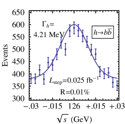
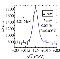
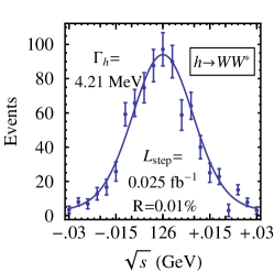
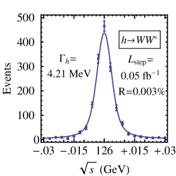
Figure 3: Number of events of the Higgs signal plus backgrounds and statistical errors expected for two different beam energy resolutions and integrated luminosities as a function of the collider energy $\sqrt{s}$ in $b\overline{b}$ and $WW^{*}$ final states with a SM Higgs $m_{h}=126~{}~{}{\rm GeV}$ and $\Gamma_{h}=4.21~{}~{}{\rm MeV}$. Detector backgrounds are not included, see more discussion in Sec. 3.3. These figures are taken from Ref [10].

We adopt a $\chi^{2}$ fit over the scanning points with three model-independent free parameters in the theory $\Gamma_{h},\ B$ and $m_{h}$ as in Eq. 2.1. We show our results for the SM Higgs width determination in Fig. 4 for beam resolutions, $R=0.01\%$ and $R=0.003\%$ by varying the luminosity. The achievable accuracies with the 20-step scanning scheme by combining two leading channels are summarized in Table 4 for three representative luminosities per step.

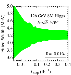
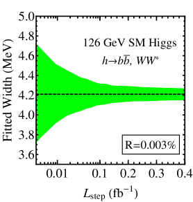
Figure 4: Fitted values and errors for the SM Higgs width versus the luminosity per step with the 20-step scanning scheme with 3-MeV step size. These figures are taken from Ref [10].

$\Gamma_{h}=4.21~{}~{}{\rm MeV}$	$L_{\rm step}$ ($~{}{\rm fb}^{-1}$)	$\delta{\Gamma_{h}}~{}(~{}{\rm MeV})$	$\delta B$	$\delta m_{h}~{}(~{}{\rm MeV})$
	$0.005$	$0.73$	$6.5\%$	$0.25$
$R=0.01\%$	0.025	0.35	3.0%	0.12
	$0.2$	$0.17$	$1.1\%$	$0.06$
	$0.01$	$0.30$	$4.4\%$	$0.12$
$R=0.003\%$	0.05	0.15	2.0%	0.06
	$0.2$	$0.08$	$1.0\%$	$0.03$

Table 4: Fitting accuracies for $\Gamma_{h}$, $B$, and $m_{h}$ of the SM Higgs with the 20-step scanning scheme with $3~{}~{}{\rm MeV}$ step size for three representative luminosities per step. Results with total integrated luminosity $0.5~{}~{}{\rm fb}^{-1}$ ($1~{}~{}{\rm fb}^{-1}$) for resolution $R=0.01\%(0.003\%)$ are in boldface. This table is taken from Ref [10].

The mass and cross section can be simultaneously determined along with the Higgs width to a high precision. The results obtained are largely free from theoretical uncertainties. The major systematic uncertainty comes from our knowledge of beam properties [6]. The uncertainty associated with the beam energy resolution $R$ will directly add to our statistical uncertainties of Higgs width. This uncertainty can be calibrated by experimentalists. On the other hand, the beam profile is unlikely to be Breit-Wigner resonance profile. Thus an additional fitting parameter of the beam energy distribution is anticipated to provide us additional knowledge about the beam energy. Our estimated accuracies are by and large free from detector resolutions. Other uncertainties associated with b tagging, acceptance, etc., will enter into our estimation of signal strength $B$ directly. These uncertainties will affect our estimation of total width $\Gamma_{h}$ indirectly through statistics, leaving a minimal impact in most cases.

3 Collider Environment

3.1 Machine Performance and Environment

A preliminary machine design for a Muon Collider Higgs Factory was presented at the Muon Accelerator Program collaboration meeting in June, 2013 [14]. This is a unique machine, designed to provide high luminosity, very small energy spread, excellent stability, and good shielding of muon beam decay backgrounds.

There are several features of the accelerator which impact the detector. The ring is 300 meters in circumference, corresponding to a 1 $\mu$s crossing interval. Beams are injected at 30 Hz and circulate for roughly 1000 turns per store. The lattice is designed both to provide high average luminosity ($1.7\times 10^{31}$ cm^-2 s^-1) and very small ($3\times 10^{-5}$) energy spread. The luminosity is achieved utilizing a quadruplet final focus with very large aperture (50 cm) quadruple magnets at the interaction region. The large beam radius, 5.6 cm bunch length, and proximity (3.5 meters) of the last quadrupole to the interaction region will require a redesign of the beam background shielding with respect to the existing $1.5~{}{\rm TeV}$ machine design. A final design will likely involve a compromise between luminosity, detector acceptance, and machine backgrounds. In this note we utilize the backgrounds that have been generated and studied for the $1.5~{}{\rm TeV}$ machine.

3.2 Energy Determination by Spin Tracking

In the present scenario the $\mu$ beams are created with a small polarization ($\approx 10$ to $20\%$) from a bias toward capture of forward $\pi\rightarrow\mu$ decays. This polarization should be substantially maintained through the cooling and acceleration systems leading to the circular storage ring of the muon collider.

While circulating in a Higgs factory storage ring, as described in the previous sections, muons continuously decay at a rate of $\cong 10^{7}$ decays per meter. As a result of the muon polarization, electrons and positrons from the muon decays will have a mean energy that is dependent upon the polarization of the muons. That polarization, $\bf{P}$ will precess as the beam rotates around the ring. The precession will, in turn, modulate the mean energy of decay electrons, and therefore provide a modulated signal at a detector capturing those decays.

The mean energy from decay electrons is:

$$<E(t)>\;=\;<(\frac{7}{20}NE_{\mu}\exp({-\alpha t}))(1+\frac{\beta}{7}\bf{P}\cos(\omega t+\phi))>$$ (3.3)

where $N$ is the initial number of $\mu$’s, $E_{\mu}$ is the $\mu$ energy, ${\alpha}$ is the decay parameter, $\beta=v/c$, $\bf{P}$ is polarization, $\phi$ is a phase, and $t$ is time in turn numbers, and:

$$\omega=2\pi\lambda(\frac{g-2}{2})\approx 2\pi\times 0.7$$ (3.4)

is the precession frequency that depends upon the muon beam energy. A detector capturing a significant number of decay electrons will have a signal modulated by $\omega$. The frequency can be measured to very high accuracy, leading to a muon beam energy measurement at the $10^{-6}$ level of precision (corresponding to $\sim 0.1~{}{\rm MeV}$), or better.

The precession observation determines the muon energy at each individual collision store. The precession signal decreases with time following the muon decay and the energy width, providing an important measurement of that width, which will assist in unfolding the Higgs width.

Raja and Tollestrup [15, 16], and Blondel [17], have analysed the polarization-based energy determination for a muon collider. Blondel established that a polarization of 5% would be sufficient to enable this measurement [18]. Simulations indicate that the muons should have an initial polarization of $(10-20)\%$ and that polarization would be maintained in cooling and acceleration.

3.3 Accelerator Backgrounds

The ability to perform physics measurements with a muon collider will largely be determined by how well one can suppress the accelerator backgrounds from the collider ring. The source of most of the accelerator backgrounds in a muon collider is associated with the decay of beam muons. Studies to date have utilized backgrounds generated for a $1.5~{}{\rm TeV}$ collider [19]. Specific backgrounds for a $126~{}{\rm GeV}$ Higgs factory have been recently calculated, [20, 21]. Both the $1.5~{}{\rm TeV}$ machine and Higgs factory designs assume $2\times 10^{12}$ muons per bunch, which will produce $4.3\times 10^{5}$ or $6\times 10^{6}$ muon decays per meter for the $1.5~{}{\rm TeV}$ and $126~{}{\rm GeV}$ machines.

The electrons resulting from muon decays will interact with the walls of the beam chamber, collimators, and shielding, producing high energy electromagnetic showers, synchrotron radiation, photonuclear interactions, and Bethe-Heitler muons. Photonuclear interactions with the nuclei of beam pipe, magnet or shielding material from energetic photons in the electromagnetic shower are the main source of the hadronic and neutron background. Neutrons are predominantly produced from photonuclear spallation processes in the giant resonance region ($14-20~{}{\rm MeV}$ incident gammas).

A preliminary study of backgrounds in a $1.5~{}{\rm TeV}$ ($750~{}{\rm GeV}$ on $750~{}{\rm GeV}$) muon collider was done utilizing MARS15, [22] [23], and G4Beamline [24] codes. The goal of the study was to calculate the accelerator-generated backgrounds that could arrive at a muon collider detector. The lattice design for this machine is described in Ref. [25], with a description of the interaction region design given in Ref. [26]. In this study the lattice was modelled at $\pm$75 m from the interaction point. Electrons from muon decays are assumed to originate at locations uniformly distributed along the $\mu^{+}$ and $\mu^{-}$ reference trajectories.

Figure 5 shows the background flux entering the detector region in a typical Muon Collider interaction [19]. Total non-ionizing background is about 10% that of the LHC, but the crossing interval is 400 times longer, resulting in high instantaneous flux. The background is very different in character than that of either the LHC or CLIC. It is dominated by soft photons and low energy neutrons emerging from the shielding surrounding the detector. A typical background event has $164~{}{\rm TeV}$ of photons, $172~{}{\rm TeV}$ of neutrons, and $184~{}{\rm TeV}$ of muons. With the exception of muons and charged hadrons the background spectrum is dominated by low energy particles. Only a small fraction of the background originates from the vicinity of the interaction region. This means that most of the decay background is out of time with respect to particles originating from the $\mu^{+}\mu^{-}$ collision.

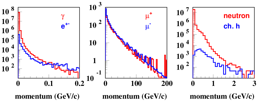
Figure 5: Energy distributions of particles entering the detector region from a MARS simulation of $1.5~{}{\rm TeV}$ Muon Collider beam backgrounds [19].

4 Detector Design

The next generation of collider detectors will emphasize precision for all sub-detector systems. In the case of a muon collider Higgs factory the $h\rightarrow b\overline{b}$ and $h\rightarrow\tau^{+}\tau^{-}$ channels require good b-tagging and vertexing capabilities. The $h\rightarrow WW^{*}$ channel will require the capability to distinguish $W$ and $Z$ vector bosons in their hadronic decay mode while $h\rightarrow\gamma\gamma$ emphasizes excellent energy and position measurement of photons .

To achieve the tracking goals we require a high solenoidal magnetic field of 5 Tesla and high precision low mass tracking. To achieve good jet resolution the electromagnetic and hadronic calorimeter have to be located within the solenoid. The machine induced background from $\mu$ decays upstream and downstream of the interaction point provides a very challenging environment; but this background is “out of time” compared to the particles from the interaction point. Therefore, for both tracker and calorimeter, good timing resolution (of order of nanoseconds) will be crucial to reduce this background to an acceptable level. This background makes shielding necessary extending into the tracker volume. Figure 6 shows an illustration of the detector as it is currently implemented in the Geant4 simulation. The tungsten shielding cone is quite visible. Here we present an idealistic conceptual design that will have to be replaced by an optimized, more realistic and cost efficient design in the future.

4.1 Tracking

To achieve the tracking goals while keeping the tracker compact we require a high solenoidal magnetic field of 5 Tesla and use silicon-based tracking with a pixelated vertex detector for high precision, low mass tracking. Fast timing and fast readout require extra power and cooling, and R&D will be necessary to achieve this while keeping detectors and support at the required low mass. Figure 7 shows the layout of the tracking and vertex detector. The vertex barrel detector is assumed to consist of 5 barrel layers with $20$ $\mu$m square pixels and $0.8\%$ radiation length per layer, the six vertex disks are assumed to utilize $50$ $\mu$m square pixels with $1.0\%$ radiation length. The four tracker barrel layers and four disk layers are assumed to have $100\times 1000$ $\mu$m short strips with $1.5\%$ radiation length per layer. The large background of non-ionizing radiation means that the silicon tracker will have to be kept cold, around $-20$ ^oC, to avoid radiation damage, increasing the detector mass. Precise timing and pixelated detectors will be crucial to a successful Muon Collider detector. Both come at a cost. Fast electronics will necessarily dissipate significant power and, in contrast to planned ILC detectors, detectors for the Muon Collider will have to be liquid (CO₂) cooled with an associated increase in mass with respect to ILC trackers.

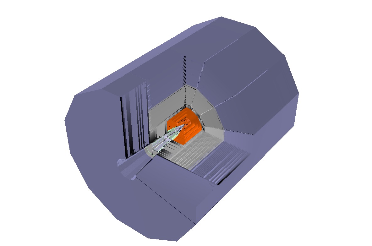
Figure 6: Illustration of the mcdrcal01 detector.

Figure 7: Layout of the vertex and tracking detector barrel and endcaps and the tungsten shielding cone.

4.2 Calorimetry

A common benchmark for ILC detectors is to distinguish W and Z vector bosons in their hadronic decay mode. This requires a di-jet mass resolution better than the natural width of these bosons and hence a jet energy resolution better than 3%. For hadron calorimetry this implies an energy resolution a factor of at least two better than previously achieved to date by any large-scale experiment.

A novel approach to achieving superior hadronic energy resolution is based on a homogeneous hadronic calorimetry (HHCAL) detector concept, including both electromagnetic and hadronic parts. This employs separate readout of the Cerenkov and scintillation light and using their correlation to obtain superior hadronic energy resolution [27, 28]. This HHCAL detector concept has a total absorption nature, so its energy resolution is not limited by the sampling fluctuations. It has no structural boundary between the ECAL and HCAL, so it does not suffer from the effects of dead material in the middle of hadronic showers. In addition there is no difference in response since the ECAL and HCAL are identical and only the segmentation differs. It also takes advantage of the dual readout approach by measuring both Cerenkov and scintillation light to correct for the fluctuations caused by the nuclear binding energy loss, so a good energy resolution for the hadronic jets can be achieved [29, 27, 28].

To improve event reconstruction we plan to use particle flow algorithms and therefore we require fine segmentation (granularity) of the calorimeter. A cost effective active material is crucial for the HHCAL detector concept and R&D is necessary to find the appropriate active materials, such as scintillating crystals, glasses or ceramics to be used to construct an HHCAL. With regards to photosensors, silicon-based photo detectors (a.k.a SiPM, MPPC) are reaching a very mature state and are becoming potential photo-transducers for hadron calorimetry for selectively detecting scintillation and Cerenkov light. The parameters and segmentation of the mcdrcal01 calorimeter are listed in Table 5.

	electromagnetic (em)	hadronic (had)	muon
Material	BGO/PbF2/PbWO4		Iron
density [g$/$cm3]	$7.13/7.77/8.29$		$7.85$
radiation length [cm]	$1.1/0.93/0.89$		$1.76$
nuclear interaction length (IA) [cm]	$22.7/22.4/20.7$		$16.8$
Number of layers	$10$	$30$	$22$
Thickness of layers [cm]	$2$	$5$	$10$
Segmentation [cm $\times$ cm]	$1\times 1$	$2\times 2$	$10\times 10$
total depths [cm]	$20$	$150$	$220$
total IA	em + had: $7.5/7.6/8.2$		$13.1$

Table 5: Properties of calorimeter and instrumented Iron flux return for barrel and endcaps for some crystal materials under consideration.

Figure 8: Wired display of a $h\rightarrow\tau^{+}\tau^{-}$ event in the mcdrcal01 detector.

Figure 9: Wired display of a $h\rightarrow\tau^{+}\tau^{-}$ event in the mcdrcal01 detector.

4.3 Software Environment

We used and extended the ALCPG [30] software suite. Using this software suite enables us to utilize existing standard reconstruction software modules for digitization, cluster algorithms, hit manipulation, tracking etc. that are part of the software package.

The ALCPG software suite consists of:

• SLIC, to simulate the detector response. SLIC is a full simulation package that uses the Geant4 Monte Carlo toolkit [31] to simulate the passage of particles through the detector. The SLIC software package uses LCDD [32] for its geometry input. LCDD itself is an extension of GDML [33]. LCDD makes it easy to quickly implement new detector concepts which is especially useful in the early stages of developing and optimizing a detector concept .

• lcsim.org [34], is a reconstruction and analysis package for simulation studies for the international linear collider. It is entirely developed in Java for ease of development and cross-platform portability.

• JAS3[35] is a general purpose, open-source data analysis framework. The following features are provided in the form of plug ins:

  • LCIO Event Browser [36].

  • WIRED 4 [37] is an extensible experiment independent event display.

  • AIDA compliant analysis system. It provides tools for plotting of 1d, 2d and 3d histograms, XY plots, scatterplots etc. and fitting (binned or unbinned) using an extensible set of optimizers including Minuit.

4.4 Background Rejection Techniques

The fact that much of the background is soft and out of time gives us two handles on the design of an experiment that can cope with the high levels of background. Timing is especially powerful. The local gate $t=0$ is defined as the time when a relativistic particle emerging from the interaction point arrives at the detector. Therefore a very tight cut can be made, still preserving the bulk of the tracks of interest. A $3$ ns cut rejects two orders of magnitude of the overall background and about four orders of magnitude of neutron background.

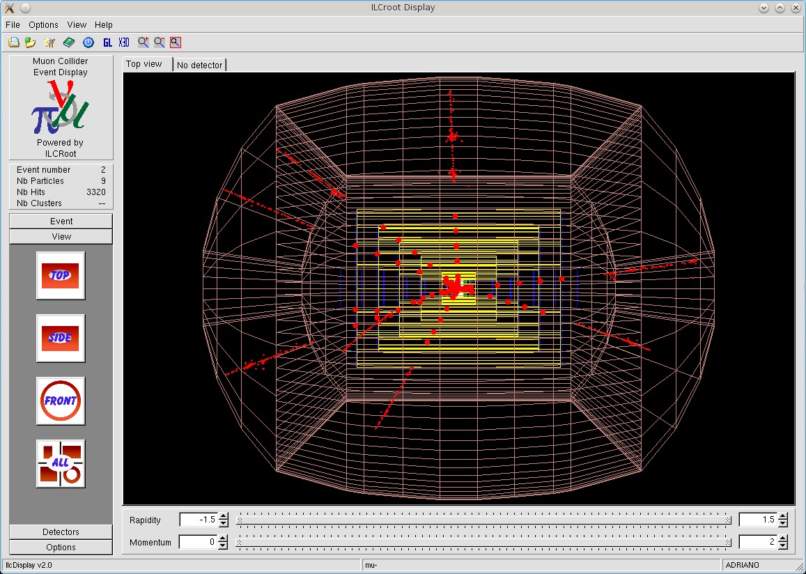
Figure 10: 10 muons from IP displayed in the ILCroot detector developed for these studies.

A study of timing for hits produced in vertex (VXD) and tracker silicon detectors by $0.75\times 0.75$ TeV Muon Collider background particles and IP muons was done recently and reported in [38]. The ILCroot simulation framework [39] was utilized. The layout of the VXD and Tracker is based on an evolution of SiD and SiLC trackers in ILC and developed by the ILCroot group (see detail in [40]). In the analysis the time of flight (TOF) of hits given relative to the bunch crossing time was recalculated relative to $T0$, the time of flight for a photon from interaction point (IP) ($x=0$, $y=0$, $z=0$) to the detector plane. Detector electronics would likely digitize and time stamp hits within a larger ($\approx 10$ ns) window to allow for fitting of slow heavy particles using TOF as a fitting parameter. The implementation of such time cuts can reduce the occupancy of the readout hits in VXD and Tracker layers to the level acceptable for efficient tracking of physics tracks as was shown in [40].

Figure 11 shows IP muon hit inefficiency and fraction of hits from background particles versus the timing gate width at 0.5 ns hit resolution time. As we can see, a timing gate width of 4 ns can provide a factor of 300-500 background rejection keeping efficiency of hits from IP muons higher than 99%.

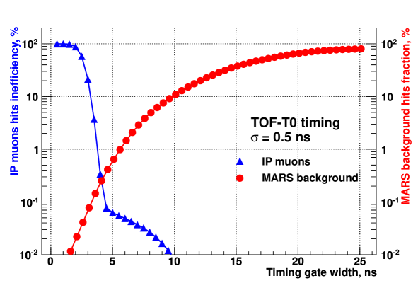
Figure 11: Inefficiency of IP muon hits and fraction of 1.5 TeV collider MARS background particles hits in the VXD and Tracker Si detectors versus width of timing gate at the hit time resolution $\sigma=0.5$ ns.

Calorimeter background Energy				Tracker Background hits
Type	Energy before cuts (TeV)	Energy after 2 ns cut (GeV)	Rejection (2 ns cut)	Radius (cm)	Rejection (1 ns cut)
EM	170	404	$2.4\times 10^{-3}$	20	$1.2\times 10^{-3}$
Muons	185	47	$0.25\times 10^{-3}$	46	$0.8\times 10^{-3}$
Mesons	7	51	$7.5\times 10^{-3}$	72	$1.1\times 10^{-3}$
Baryons	178	386	$2.1\times 10^{-3}$	97	$0.6\times 10^{-3}$

Table 6: Rejection of beam background calorimeter energy and tracker hits for a 1.5 TeV Muon Collider with timing windows with respect to time of flight from the primary vertex of 2 and 1 ns respectively.

Timing is also crucial for background rejection in the calorimeter. A calorimeter design studied by R. Raja [41] that combines fast timing with the reconstruction ability of pixelated calorimeters being studied for particle flow. In this design a pixelated imaging sampling calorimeter with $200$ $\mu$m square cells and a 2 ns “traveling trigger” gate referenced to the time of flight with respect to the beam crossing is used to reject out-of-time hits. This sort of calorimeter can also implement compensation by recognizing hadronic interaction vertices and using the number of such vertices to correct the energy. Initial estimates of the resolution of such a compensated calorimeter is $60\%/\sqrt{E}$. In contrast to relativistic tracks and electromagnetic showers, hadronic showers can take significant time to develop. Initial studies of a dual readout total absorption calorimeter for the Muon Collider also show that resolution lost to a fast time gate can be regained by utilizing a dual readout correction. A summary of the tracking and pixelated calorimetry background rejection factors for a 1.5 TeV collider are shown in Table 6.

We have learned that tracking is feasible in a Muon Collider detector. Calorimetery is more challenging, but progress is being made on calorimeter concepts that appear to meet the physics needs.

5 Detector Simulation Studies of Higgs Physics

We will presently utilize the detector model described in the previous section to discuss $s$-channel resonant Higgs boson production and standard model backgrounds at the Muon Collider Higgs Factory. We assume that we are operating at center-of-mass energy $\sqrt{s}=M_{h}\approx 125~{}{\rm GeV}$ with a beam energy resolution of $\delta E\sim 3.54~{}{\rm MeV}$ ($R=0.004\%$). PYTHIA-generated standard model Higgs boson and background events were used at the generator level to identify and evaluate important channels for discovery and measurement of the Higgs mass, width, and branching ratios.[11].

The $h\rightarrow b\overline{b}$ and $h\rightarrow WW^{*}$ channels are the most useful for locating the Higgs peak (see Section 2). With an integrated luminosity of $\sim 4.2\ fb^{-1}$ we can measure a $125~{}{\rm GeV}$ Higgs boson mass accurately to within $\sim 0.06~{}{\rm MeV}$, and the total width to within $\sim 0.18~{}{\rm MeV}$. These results demonstrate the value of the large, resonant Higgs cross-section and the narrow beam energy resolution achievable at a muon collider.

5.1 Including Backgrounds

The most significant background for $s$-channel resonance Higgs production at a muon collider is the production of $Z$-bosons. The Higgs cross section, smeared by a $3.54~{}{\rm MeV}$ beam is $31.5\,{\rm pb}$ but first-order initial state radiation corrections bring the effective cross section to $16.7\,{\rm pb}$. The cross section of the $Z$ background is $376\,{\rm pb}$, but $\sim 20\%$ of these $Z$ decays into pairs of neutrinos and a photon, bringing the cross section to $301.4\,{\rm pb}$. This cross section remains essentially flat in the region around the Higgs peak and will be treated as such in this report.

Figure 12 shows simulated data of a scan across a $125.0~{}{\rm GeV}$ Higgs peak counting all events except for $Z^{0}\rightarrow\nu_{\ell}\overline{\nu_{\ell}}$. This is fit to a Breit-Wigner distribution, convoluted with a Gaussian with three free parameters, $\Gamma_{h}$, $M_{h}$ and Br$(h\rightarrow X)$. The fixed parameters are the background cross section, $\sigma(Z^{0}\rightarrow X)$, the beam width $\sigma_{beam}$ and the total integrated luminosity $\mathcal{L}$. The fit gives a width of $4.3\pm 0.6~{}{\rm MeV}$, an error in the mass measurement of $0.46\pm 0.16~{}{\rm MeV}$ and a branching ratio of $0.96\pm 0.10$.

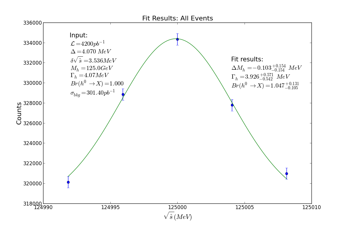
Figure 12: Simulated event counts for a scan across a $125.0~{}{\rm GeV}$ Higgs peak with a $3.54~{}{\rm MeV}$ wide Gaussian beam spread, counting all events except for $Z^{0}\rightarrow\nu_{\ell}\overline{\nu_{\ell}}$ decays. Data is taken in a range of $\pm 8.14~{}{\rm MeV}$ centered on the Higgs mass in bins separated by the Higgs FWHM (Full width at half maximum) of $4.07~{}{\rm MeV}$. Total integrated luminosity is $4.2~{}{\rm fb}^{-1}$. Event counts are calculated as Poisson-distributed random variables and the data is fit to a Breit-Wigner convoluted with a Gaussian peak plus linear background. Fitted values of the free parameters are in Table 8.

Fortunately, this background is reducible. The $s$-channel resonant production of Higgs bosons only happens within a few $~{}{\rm MeV}$ of the peak. However, $Z$ bosons are produced in several different processes with a wide range of masses, as seen in Figure 13. At an $s$-channel Higgs factory muon collider, $Z$ bosons are primarily produced as real, on-shell bosons along with an intial state photon that makes up the difference in energy between the Higgs s-channel and the $Z$ mass (Fig. 14(b)). There is also a small number of very low mass $Z$ bosons produced in a Drell-Yan process. The only events that are theoretically indistinguishable from Higgs events are those where a virtual $Z$ is produced at the center of mass energy and decays into a channel shared with the Higgs (Fig. 14(a)).

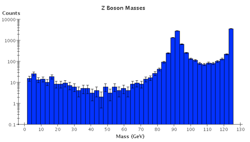
Figure 13: $Z$ boson masses in 10,000 PYTHIA-simulated $\mu^{+}\mu^{-}\rightarrow Z$ events at $\sqrt{s}=125.0~{}{\rm GeV}$. The low-mass region is dominated by the Drell-Yan process. There is a peak around the $Z$ mass where intial-state Bremsstrahlung radiation allows the creation of an on-shell Z. The third region of interest is the peak at $125~{}{\rm GeV}$, the center of mass energy. This represents a process with no initial state radiation where the off-shell Z’s produced are indistinguishable from the Higgs.

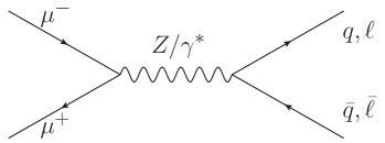
(a) Irreducible background: $\mu^{+}\mu^{-}\rightarrow Z/\gamma^{*}$ with $M_{Z^{*}}=\sqrt{s}$.

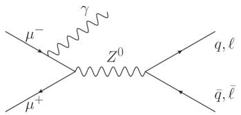
(b) Reducible background: $\mu^{+}\mu^{-}\rightarrow Z^{0},\gamma$ with $M_{Z^{0}}<m_{h}$.

Figure 14: Standard Model backgrounds at a $\mu^{+}\mu^{-}$ collider operating at $\sqrt{s}=126~{}{\rm GeV}$

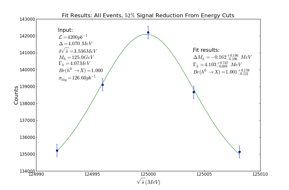
Figure 15: Simulated event counts for a scan across a $125.0~{}{\rm GeV}$ Higgs peak with a $3.54~{}{\rm MeV}$ wide Gaussian beam spread, counting all events with a total energy of at least $98.0~{}{\rm GeV}$ visible to the detector. Data is taken in a $8.14~{}{\rm MeV}$ range centered on the Higgs mass in bins separated by the beam width of $4.2~{}{\rm MeV}$. Event counts are calculated as Poisson-distributed random variables and the data is fit to a Gaussian peak plus linear background. The fit width is $4.4\pm 0.8~{}{\rm MeV}$ and the error in the mass measurement is $0.1\pm 0.2~{}{\rm MeV}$.

Before looking into how the kinematics of these events might differ from Higgs events, the simple thing to do is a cut on the total energy potentially visible to the detector. This is accomplished by summing the energies of all final state particles which pass a $\cos{\theta}<0.94$ cut and finding the energy cut which maximizes $S/\sqrt{B}$. The $\cos{\theta}$ cut is effective because most of the high-energy initial state radiation is colinear with the beam. We use a cut of $E_{total}>98.0~{}{\rm GeV}$, which selects 79.2% of the Higgs signal events and 41.9% of the $Z$ background. This results in an effective Higgs cross section of $22.4\,{\rm pb}$ and a background of $126.4\,{\rm pb}$.. Figure 15 shows simulated data using these results, with a fitted width of $5.57\pm 1.33~{}{\rm MeV}$ and an error in the mass measurement of $-0.02\pm 0.14~{}{\rm MeV}$. This simple cut has already proven to be a marginal improvement but there is much more that can be done by focusing on individual decay channels.

Decay Mode	Bkgr.	$h$
	$\sigma$ (pb)	BR	$\sigma$ (pb)
$u\overline{u}$,$d\overline{d}$,$s\overline{s}$	56.0	0.0003	0.01
$c\overline{c}$	20.3	0.029	1.1
$b\overline{b}$	57.2	0.577	9.6
$e^{+}e^{-}$	9.2	—	—
$\mu^{+}\mu^{-}$	4.8	—	—
$\tau^{+}\tau^{-}$	9.2	0.063	2.4
$\nu_{\ell}\overline{\nu_{\ell}}$	75.2	—	—
$gg$	—	0.086	3.2
$\gamma\gamma$	27.6	0.002	0.07
$WW^{*}$	0.001	0.215	8.0
$Z^{0}Z^{0}$	—	0.026	0.97
Total:	259.6	1.0	25.5

Table 7: Branching fractions and effective cross sections for Standard Model decay modes of Higgs and $Z$ bosons. Higgs cross sections are calculated as the peak value of the Higgs peak Breit-Wigner convoluted with a Gaussian of width $3.54~{}{\rm MeV}$ to simulate the effect of beam smearing. The inclusion of initial state radiation effects and full one loop corrections will further reduce the cross sections for Higgs production by a factor of 0.53; resulting in a total Higgs cross section of $13.6{\rm~{}pb}$. Background cross sections are taken from PYTHIA 6.4 event generation output.

5.1.1 $h\rightarrow b\overline{b}$

Table 7 compares the branching ratios and cross sections of the $Z$ background with the Higgs signal. The largest Higgs decay channel is $h\rightarrow b\overline{b}$, which makes up 58% of Higgs decays at this mass, a branching fraction proportionally large to $Br(Z^{0}\rightarrow b\overline{b})=15.2\%$. We assume a b-tagging efficiency and purity of 1, so the cross sections for the decays are 16.5 and 57.2 pb, respectively. The fitted values for the mass, width and branching ratio of the Higgs using b-tagging are shown in Table 8.

In both signal and background the visible energy spectrum is very similar to the spectrum of the combined channels, so the same total energy cut of $E_{tot}>98.0~{}{\rm GeV}$ maximizes $S/\sqrt{B}$. Cuts on the event shape, the magnitude of the thrust and major axis, can further enhance the signal. The event shape is calculated by finding the axis which maximizes the sum of all particle momenta projected onto a single axis, called the ‘thrust axis’. This is then repeated for an axis perpendicular to the first and then a third orthogonal to both. The thrust is the normalized sum of the projection of all particle momenta against the thrust axis and the major axis value is the normalized sum of the projections against the secondary axis. Because the Higgs is never created in events with significant beamstrahlung it is always produced with low momentum. $Z$ bosons produced with mass lower than the beam center-of-mass energy are ‘boosted’ by the beamstrahlung photon. This boost lowers the thrust and raises the major axis values, so it is a useful indicator for channels with particular event shape profiles.

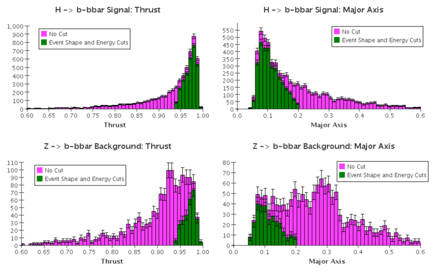
Figure 16: Effects of event shape and energy cuts on Higgs $b\overline{b}$ signal and background. Cuts were made by selecting events with total energy $E_{tot}>98.0~{}{\rm GeV}$ visible to the detector, thrust between 0.94 and 1.0 and major axis between 0.0 and 0.2. The signal is reduced to 52% and the background to 15%.

Figure 16 shows the signal and background thrust and major axes before and after cutting on the total energy and event shape values. The cuts were made by selecting events with $E_{tot}>98.0~{}{\rm GeV}$, thrust values between 0.94 and 1.0 and major axis values between 0.0 and 0.20. We continue to assume perfect b-tagging. These cuts reduce the $b\overline{b}$ signal by 52% and the background by 15%, bringing the effective cross sections to 8.64 and 8.45 pb respectively. This improves the $S/\sqrt{B}$ over simple energy cuts or b-tagging alone. Figure 17 shows a simulated scan of the Higgs peak with a fit to a Breit-Wigner convoluted with a Gaussian.

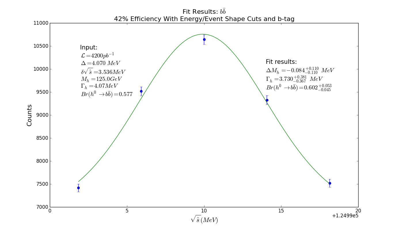
Figure 17: Simulated event counts for a scan across a $125.0~{}{\rm GeV}$ Higgs peak with a $4.2~{}{\rm MeV}$ wide Gaussian beam spread, counting $X\rightarrow b\overline{b}$ events with a total energy of at least $98.0~{}{\rm GeV}$ visible to the detector and cutting on event shape parameters. Data is taken in a $60~{}{\rm MeV}$ range centered on the Higgs mass in bins separated by the beam width of $4.2~{}{\rm MeV}$. Event counts are calculated as Poisson-distributed random variables and the data is fit to a Breit-Wigner convoluted with a Gaussian plus linear background. The fit width is $4.78\pm 0.48~{}{\rm MeV}$, the error in the mass measurement is $0.01\pm 0.05~{}{\rm MeV}$ and the branching ratio is measured at $0.271\pm 0.001$. Total luminosity is $1000\,{\rm pb}^{-1}$, or $71.4\,{\rm pb}^{-1}$ per point.

5.1.2 $h\rightarrow WW^{*}$

There are several channels with very little physics background that are of importance, despite their smaller cross sections. One of these is the $h\rightarrow WW^{*}$ decay mode, with a branching fraction of 0.226 (cross section 6.39 pb) and no real background from the corresponding $Z$ decays. The $W$ boson decays into a charged lepton and corresponding neutrino 32.4% of the time, with effectively equal rates for each type of lepton. The majority of the remaining branching fraction is the decay into pairs of light quarks. While it is certainly possible to reconstruct $W$ bosons from four-jet events, in this report we focus on the decays with missing energy in the form of neutrinos since they can be identified by the presence of one or two isolated leptons and missing energy and are the most common. Further study will be required for a detailed analysis of the four-jet case. Since the $W$ boson decays into a lepton and neutrino 32.4% of the time and we require at least one such decay between a pair of $W$’s, these make up 54.3% of $WW^{*}$ events. Thus the theoretical cross section is 6.39 pb with virtually no background.

Because the detector will have a non-sensitive cone, there will be a small amount of ‘fake’ background, eg. when the photon in the decay $\mu^{+}\mu^{-}\rightarrow Z^{0}+\gamma\rightarrow\ell^{+}+\ell^{-}$ boosts the two leptons and disappears into the cone as missing energy. It is difficult to estimate the true background from processes such as these, but given the low branching ratios of $Z^{0}$ to lepton pairs and the kinematic and geometric constraints for ‘fake’ background, it is safe to assume that the background will be fairly low in this channel. Therefore we use a cross-section of 0.051 pb.

5.1.3 $h\rightarrow\tau^{+}\tau^{-}$

The $\tau^{+}\tau^{-}$ channel is dominated by the background, but the Higgs branching ratio of 0.071 is not insignificant. The $Z^{0}\rightarrow\tau^{+}\tau^{-}$ process has a branching ratio of $0.034$, giving it an effective cross section of $12.8$ pb, compared to the $2.01$ pb cross section for the Higgs. However, the boost given to the lower mass $Z$ bosons means the background can be further distinguished using total energy and event shape parameters.

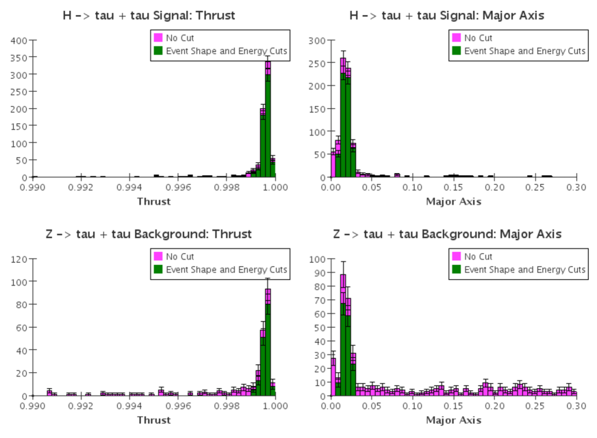
Figure 18: Effects of event shape and energy cuts on Higgs $\tau^{+}\tau^{-}$ signal and background. Cuts were made by selecting events with total energy $E_{tot}>60.0~{}{\rm GeV}$ visible to the detector, thrust between 0.999 and 1.0 and major axis between 0.07 and 0.032. The signal is reduced to 78% and the background to 39%.

The $\tau$ is a short-lived particle and every $\tau$ decay channel involves the production of a $\tau$ neutrino. This makes the total visible energy less useful as a cut parameter than it was for $b\overline{b}$, since there are random amounts of missing energy. We require at least $60.0~{}{\rm GeV}$ to be visible because background dominates below this value due to boosted $Z$’s. Event shape parameters, however, are very useful here since $\tau$ decays typically do not create a widespread shower. We require the thrust to be between 0.999 and 1.0 and the major axis to be between 0.007 and 0.03. This cut reduces the signal to 78% of its original value and the background to 39%, bringing the Higgs cross section to 1.58 pb and the background to 4.97 pb, as seen in Figure 18. The cut is specific enough that it is not necessary to assume anything else about the events, such as a perfect $\tau^{+}\tau^{-}$ tag. Fewer than 0.2% of the Higgs decays that pass the cut are not $\tau^{+}\tau^{-}$ events and only 6.4% of the background events that pass are misidentified. The effective background cross section above is calculated from all the events which pass the cut.

5.1.4 $h\rightarrow c\overline{c}$

With an integrated luminosity of $\sim 1~{}{\rm fb}^{-1}$ one expects $\sim 23,000$ produced Higgs bosons, implying $\sim 800$ $h\rightarrow c\overline{c}$ decays and $\sim 13,000$ $h\rightarrow b\overline{b}$ decays.

To obtain a sensitive $c\overline{c}$ branching fraction implies the need to reject the $b\overline{b}$ background by a factor of 20 or more. Additionally, there is a long tail of $c\overline{c}$ and $b\overline{b}$ coming from $Z$ decays. This produces a background of 19 pb under the $h$ peak [12], and it therefore generates an additional $\sim 19,000$ events.

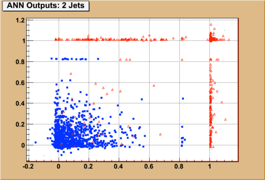
Figure 19: The two-jet neural net output plane for $\mu^{+}\mu^{-}\rightarrow h\rightarrow 2{\rm~{}heavy~{}quark~{}jets}$ events in the detector. True $c$-jets are shown as blue squares, while the true $b$-jets are shown as red triangles.

Observing the $h$ peak in $c\overline{c}$ decays should still be possible, but the background from $Z$-decays will be the dominant one after rejection of the $h\rightarrow b\overline{b}$ decays. As shown in Fig. 19, excellent separation of charm and bottom jets is also possible for Higgs decays at the muon collider. A simple estimate of $S/\sqrt{B}$ implies an observation of the $h\rightarrow c\overline{c}$ signal will be possible at the $\sim 5$ to $\sim 6$ $\sigma$ level at the muon collider Higgs factory [13].

Channel $\mu^{+}\mu^{-}\rightarrow h\rightarrow X$ $\mu^{+}\mu^{-}\rightarrow X$ $S/\sqrt{B}$ Br $\sigma$ (pb) Br $\sigma$ (pb) Total 1.0 $\sigma_{s}$ 16.7 1.0 $\sigma_{b}$ 376.0 55.8 $\sigma_{eff}$ 13.2 $\sigma_{eff}$ 126.6 76.0 $b\overline{b}$ 0.577 $\sigma_{s}$ 9.6 0.152 $\sigma_{b}$ 57.2 82.3 $\sigma_{eff}$ 4.0 $\sigma_{eff}$ 6.9 98.7 $WW^{*}$ 0.215 $\sigma_{s}$ 3.6 5e-4 $\sigma_{b}$ — — $\sigma_{eff}$ 1.9 $\sigma_{eff}$ 0.001 3,894 $\tau^{+}\tau^{-}$ 0.063 $\sigma_{s}$ 1.1 0.042 $\sigma_{b}$ 12.8 19.9 $\sigma_{eff}$ 0.9 $\sigma_{eff}$ 5.1 23.0 $c\overline{c}$ 0.029 $\sigma_{s}$ 0.48 0.118 $\sigma_{b}$ 44.4 12.6 $\sigma_{eff}$ 0.44 $\sigma_{eff}$ 42.9 11.9 $\gamma\gamma$ 0.002 $\sigma_{s}$ 0.03 0.13 $\sigma_{b}$ 27.6 0.37 $\sigma_{eff}$ 0.02 $\sigma_{eff}$ 27.6 0.6

Table 8: Branching fractions, cross sections before and after cuts and $S/\sqrt{B}$ for the channels studied. We assumed an integrated luminosity of $4.2~{}{\rm fb}^{-1}$ for determining the $S/\sqrt{(}B)$ values. Background cross sections were calculated with PYTHIA 6.4 simulations.

Channel $\Gamma_{H\rightarrow X}(MeV)$ $\Delta M_{H}(MeV)$ $Br(h\rightarrow X)$ Total Raw $3.9\pm 0.6$ $-0.10\pm 0.15$ $1.05\pm 0.13$ Cut $4.1\pm 0.7$ $-0.16\pm 0.19$ $1.0\pm 0.16$ $b\overline{b}$ Raw $4.3\pm 0.5$ $0.1\pm 0.1$ $0.55\pm 0.05$ Cut $3.7\pm 0.4$ $-0.08\pm 0.1$ $0.60\pm 0.05$ $WW^{*}$ Raw $---$ $---$ $---$ Cut $3.9\pm 0.2$ $0.06\pm 0.07$ $0.22\pm 0.01$ $\tau^{+}\tau^{-}$ Raw $3.5\pm 2.0$ $0.00\pm 0.5$ $0.07\pm 0.05$ Cut $4.5\pm 1.5$ $-0.1\pm 0.4$ $0.06\pm 0.02$

Table 9: Fitted values of Higgs decay width, mass and branching ratio from simulated data. Mass values are the difference between the measured mass and the true mass of $126,000~{}{\rm MeV}$. Total integrated luminosity was $4.2~{}{\rm fb}^{-1}$, or $840\,{\rm pb}^{-1}$ per data point.

5.2 Combining Channels

Channel	$\delta M_{H}$ (MeV)	$\delta\Gamma_{H}$ (MeV)	$\delta Br(h\rightarrow X)$
$b\overline{b}$	0.1	0.4	0.05
$WW^{*}$	0.07	0.2	0.01
Combined	0.06	0.18	—

Table 10: Accuracy of fitting parameters for simulated Higgs data using individual and combined channels.

To measure the Higgs mass and total width more precisely, we took advantage of both the $b\overline{b}$ and the $WW*$ channels. We did this by simulating data for both channels and taking their average, weighted by the uncertainty in the fits, with results shown in Table 10. For example, the formula used for the width was:

$$\overline{\Gamma}_{H}=\frac{\delta\Gamma_{b\overline{b}}}{\delta\Gamma_{b\overline{b}}+\delta\Gamma_{WW^{*}}}\Gamma_{WW^{*}}+\frac{\delta\Gamma_{WW*}}{\delta\Gamma_{b\overline{b}}+\delta\Gamma_{WW^{*}}}\Gamma_{b\overline{b}}$$ (5.5)

$$\delta\overline{\Gamma}_{H}^{2}=\frac{\delta\Gamma_{b\overline{b}}^{2}\delta\Gamma_{WW*}^{2}}{\delta\Gamma_{b\overline{b}}^{2}+\delta\Gamma_{WW*}^{2}}$$ (5.6)

5.3 Potential to Resolve Nearly Degenerate Higgs Bosons

The Higgs line-shape scanning process not only provides high precision for the Higgs boson total width, but also high precision for the Higgs mass. Sub MeV level precision can be achieved as show in Table 4. This implies that the muon collider will be an ideal machine to break the mass degeneracies between Higgs bosons. In this section, we discuss this potential of the muon collider.

There are theoretical speculations that the LHC Higgs signal may be a combination of two nearly degenerate Higgs-like bosons [42, 43, 44, 45, 46, 47, 48]. This could happen in some models, for example, two Higgs doublet models (2HDM) [42, 43, 44], 2HDM plus 1 singlet models, as well as next-to-minimal-supersymmetric-model [45, 46, 47]. A putative $\sim 1~{}{\rm GeV}$ level degeneracy could be easily resolved at an early stage of the muon collider program, when the Higgs mass window is determined, as described in Sec.2.2. However, we can go much further, and we discuss presently the $\sim 1~{}{\rm MeV}$ level mass degeneracy resolution achievable at a muon collider.

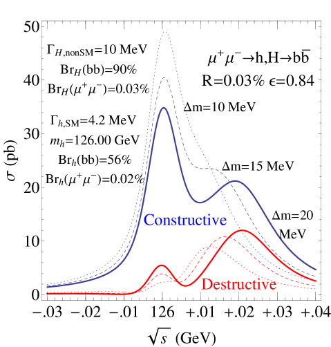
Figure 20: Resolving highly degenerate Higgs bosons at the muon collider through scanning. The b-tagging efficiency is assumed to be $60~{}\%$, and the acceptance $\epsilon$ is thus $0.84$ with at least one b-jet tagged. The solid, dashed and dotted lines represent mass splittings of the Higgs bosons, $20~{}~{}{\rm MeV},~{}15~{}~{}{\rm MeV}$ and $10~{}~{}{\rm MeV}$. The blue and red curves represent constructive and destructive interferences, respectively.

A naive expectation is that the muon collider could resolve the mass degeneracy to sub MeV level, as it does for the single Higgs boson mass fitting. However, this is way below the beam energy spread and the Higgs boson total width. The latter means the interference effect between these two highly degenerate Higgs bosons has to be taken into account at the muon collider. We demonstrate this resolution in Fig. 20 for $\mu^{+}\mu^{-}\rightarrow h,H\rightarrow b\overline{b}$. We fix the SM Higgs Boson at $126~{}~{}{\rm GeV}$ with total width $4.2~{}~{}{\rm MeV}$. We set the other Higgs total width at $10~{}~{}{\rm MeV}$ and the branching fractions to $b\overline{b}(\mu^{+}\mu^{-})$ $90\%(0.03\%)$. This corresponds to a non-SM doublet Higgs with $\tan\beta$ around $2$ in Type II 2HDM, as well as (more likely) a larger $\tan\beta$ with a significant mixing with additional singlet. We choose three different masses from $126.01~{}~{}{\rm GeV}$ to $126.02~{}~{}{\rm GeV}$ and demonstrate both constructive and destructive interferences.

This mass degeneracy resolution depends on many factors. The optimal scenario would be both Higgs bosons having the same total width and signal strength. Instead of this optimal scenario, our choice in Fig. 20 has both Higgs bosons with the same order of strength and total width. We can see that shape fitting is necessary to resolve a $\sim 10~{}~{}{\rm MeV}$ degeneracy. As a result, we argue the muon collider could a resolve mass degeneracy to the level of these Higgs bosons’ total widths.

There are other ways to resolve the mass degeneracy at the muon collider. For example, for 2HDM and related models, the other Higgs is expected not to have suppressed couplings to the vector bosons. One could fit the mass from the $WW^{*}$ mode to sub MeV level for the SM-like Higgs and fit the mass from the $b\overline{b}$ mode to a similar level. These two fits would have different best fit masses and thus resolve the degeneracy. This scenario dependent method has the potential of resolving the mass degeneracy to the MeV level.

The muon collider Higgs factory is an ideal place to resolve the mass degeneracy of Higgs bosons. Its resolution is at the level of the Higgs bosons’ total widths. This excellent mass degeneracy resolution can also be applied to the future upgrade of the muon collider for the energy frontier, where in many 2HDM and related models the heavier Higgs and CP-odd Higgs are highly degenerate [49].

5.4 Testing the CP Property

While the newly discovered Higgs boson seems to behave a SM-like, the nature of its couplings to fermions is largely unknown. Denote a generic Higgs scalar ($H$) to couple to a pair of fermions ($\psi$) by

$$H\ \overline{\psi}(a+ib\gamma_{5})\psi.$$ (5.7)

The most ideal means for determining the CP nature of a Higgs boson at the muon collider is to employ transversely polarized muons [50, 51]. For $h$ production at a muon collider with muon coupling given by the form in Eq. (5.7), the cross section takes the form

$$\overline{\sigma}_{h}(\zeta) = \overline{\sigma}_{h}^{0}\left(1+P_{L}^{+}P_{L}^{-}+P_{T}^{+}P_{T}^{-}\left[{a^{2}-b^{2}\over a^{2}+b^{2}}\cos\zeta-{2ab\over a^{2}+b^{2}}\sin\zeta\right]\right)$$ (5.8)

$$= \overline{\sigma}_{h}^{0}\left[1+P_{L}^{+}P_{L}^{-}+P_{T}^{+}P_{T}^{-}\cos(2\delta+\zeta)\right]\,,$$

where $\overline{\sigma}_{h}^{0}$ is the unpolarized convoluted cross section, $\delta\equiv\tan^{-1}(b/a)$, $P_{T}$ ($P_{L}$) is the degree of transverse (longitudinal) polarization, and $\zeta$ is the angle between the $\mu^{+}$ and $\mu^{-}$ transverse polarizations. Only the $\sin\zeta$ term is genuinely CP-violating, but the $\cos\zeta$ term also provides significant sensitivity to $a/b$. Ideally, one would like to isolate ${a^{2}-b^{2}\over a^{2}+b^{2}}$ and ${-2ab\over a^{2}+b^{2}}$ by running at fixed angles $\zeta=0,\pi/2,\pi,3\pi/2$ and measuring the asymmetries. Taking $P_{T}^{+}=P_{T}^{-}\equiv P_{T}$ and $P_{L}^{\pm}=0$, we form two observables

$${\cal A}_{I} \equiv {\overline{\sigma}_{h}(\zeta=0)-\overline{\sigma}_{h}(\zeta=\pi)\over\overline{\sigma}_{h}(\zeta=0)+\overline{\sigma}_{h}(\zeta=\pi)}=P_{T}^{2}{a^{2}-b^{2}\over a^{2}+b^{2}}=P_{T}^{2}\cos 2\delta\,,$$

$${\cal A}_{II} \equiv {\overline{\sigma}_{h}(\zeta=\pi/2)-\overline{\sigma}_{h}(\zeta=-\pi/2)\over\overline{\sigma}_{h}(\zeta=\pi/2)+\overline{\sigma}_{h}(\zeta=-\pi/2)}=-P_{T}^{2}{2ab\over a^{2}+b^{2}}=-P_{T}^{2}\sin 2\delta\,.$$

If $a^{2}+b^{2}$ is already well determined from its overall coupling strength, and the background is known depending on the specific final state, then the fractional error in these asymmetries can be approximated as ${\delta{\cal A}/{\cal A}}\propto{1/P_{T}^{2}\sqrt{L}}$ [51], which points to the need for the highest possible transverse polarization, even if some sacrifice in $L$ is required.

A crude estimate [51] showed that with $P_{T}\sim 40\%$ and $L=0.1~{}{\rm fb}^{-1}$ delivered on a scalar resonance, a 30% ($1\sigma$) measurement on $b/a$ is possible. In reality the precession of the muon spin in a storage ring makes running at fixed $\zeta$ impossible. Detailed studies will be needed to achieve quantitative conclusions.

References

- [1]
- [2] Y. Alexahin, et al., arXiv:1307.6129 [hep-ph].
-
[3]
G. Aad et al. , ATLAS Collaboration, “Observation of a New Particle in the Search for the
Standard Model Higgs Boson with the ATLAS Detector at the LHC,” arXiv:1207.7214 [hep-ex], Phys. Lett. B716, 1 (2012);
Chatrchyan et al. , CMS Collaboration, “Observation of a new boson at a mass of GeV with the CMS experiment at the LHC,” arXiv:1207.7235 [hep-ex], Phys. Lett. B716, 30 (2012). - [4] S. Weinberg, Phys. Rev. Lett. 19, 1264 (1967).
-
[5]
M. Palmer, “Muon Accelerators: An Integrated Path to Intensity and Energy Frontier Physics Capabilities”,
Presented at the Higgs Factory Muon Collider Workshop at UCLA, March 21-23, 2013 (unpublished)
[https://hepconf.physics.ucla.edu/higgs2013/talks/palmer.pdf] -
[6]
D. Neuffer, et al. , “A Muon Collider as a Higgs Factory,” paper TUPFI056, Proceedings of the 4th International Particle Accelerator Conference (IPAC13), Shanghai, China (2013);
D. Neuffer, “The First Muon Collider - 125 GeV Higgs Factory?,” AIP Conf. Proc. 1507, 849 (2012). - [7] Yuri Alexahin, UCLA Workshop, 2013, https://hepconf.physics.ucla.edu/higgs2013/talks/alexahin.pdf]
-
[8]
B. Grinstein, “Higgs, Higgs impostors, Higgs lookalikes and all that”,
Presented at the Higgs Factory Muon Collider Workshop at UCLA, March 21-23, 2013 (unpublished)
[https://hepconf.physics.ucla.edu/higgs2013/talks/grinstein.pdf] - [9] J. Alwall, M. Herquet, F. Maltoni, O. Mattelaer and T. Stelzer, JHEP 1106, 128 (2011) arXiv:1106.0522 [hep-ph].
- [10] T. Han and Z. Liu, Phys. Rev. D 87, 033007 (2013) arXiv:1210.7803 [hep-ph].
- [11] A. Conway and H. Wenzel, arXiv:1304.5270 [hep-ex].
-
[12]
E. Eichten, “Physics at a Muon Collider Higgs Factory”,
Presented at the Higgs Factory Muon Collider Workshop at UCLA, March 21-23, 2013 (unpublished)
[https://hepconf.physics.ucla.edu/higgs2013/talks/eichten.pdf] -
[13]
M. Purohit, “Can we observe ?”,
Presented at the Higgs Factory Muon Collider Workshop at UCLA, March 21-23, 2013 (unpublished)
[https://hepconf.physics.ucla.edu/higgs2013/talks/purohit.pdf] - [14] Y. Alexahin, Muon Accelerator Program meeting, June 2013, [https://indico.fnal.gov/getFile.py/access?contribId=18&sessionId=4&resId=0&materialId=slides&confId=6714]
- [15] R. Raja and A. Tollestrup, Physical Review D58, 013005 (1998).
- [16] R. Raja and A. Tollestrup, AIP Conf. Proc. 435, 583 (1998).
- [17] A. Blondel, Energy calibration by spin precession in Prospective Study of Muon Storage Rings at CERN, (B. Autin, , A. Blondel and J. Ellis, ed.) CERN 99-02 (1999), pp. 51-54.
- [18] A. Blondel, Muon Polarisation in the neutrino factory, NIM A451, 131-137 (2000).
- [19] N.V. Mokhov, S.I. Striganov, Physics Procedia 37, (2012) 2015-2022.
- [20] N.V. Mokhov, et al. , “Design and simulation of mu+mu- Higgs Factory machine detector interface”, UCLA Workshop, March 2013 and MAP Collaboration meeting, Fermilab, June, 2013.
- [21] S. Striganov et al. , “Higgs Factory background simulations, UCLA Workshop, March 2013 and MAP Collaboration meeting, Fermilab, June, 2013.
- [22] The MARS Code System, [http://www-ap.fnal.gov/MARS]
- [23] N.V. Mokhov, ”The Mars Code System User’s Guide”, Fermilab-FN-628 (1995); N.V. Mokhov, S.I. Striganov, ”MARS15 Overview”, Proc. of Hadronic Shower Simulation Workshop, Fermilab,September 2006, AIP Conf. Proc. 896, pp 50-60 (2007).
- [24] T.J. Roberts and D. Kaplan, G4beamline Simulation Program for Matter Dominated Beamlines”, Proc. of PAC07, p3468, also see [http://g4beamline.muonsinc.com].
-
[25]
Y. Alexahin et al., “Conceptual Design of the Muon
Collider Ring Lattice”, Proc. of
IPAC’10, Kyoto (2010).
[http://accelconf.web.cern.ch/AccelConf/IPAC10/papers/tupeb021.pdf] -
[26]
Y. Alexahin et al., “Muon Collider Interaction
Region Design”, Proc. of IPAC’10,
Kyoto, (2010).
[http://accelconf.web.cern.ch/AccelConf/IPAC10/papers/tupeb022.pdf] - [27] A. Para, talk given in International Linear Collider Workshop, Chicago (2008).
- [28] H. Wenzel, talk given at the 2009 Linear Collider Workshop of the Americas, Albuquerque, (September 2009).
- [29] The Dream Collaboration, R. Wigmans, Recent Results from the Dream Project, in Proceed- ings of XIII International Conference on Calorimetry in Particle Physics, Ed. M. Fraternali et al., IOP Conference Series Volume 160 (2009) 012018, and N. Akchurin et al., Nucl. Instr. and Meth. A582 (2007) 474, A584 (2008) 304, A593 (2008) 530, A595 (2008) 359 and A598 (2008) 710.
- [30] [http://physics.uoregon.edu/~lc/alcpg/].
-
[31]
The two main reference papers for Geant4 are published in Nuclear
Instruments and Methods in Physics Research A 506 (2003) 250-303,
and IEEE Transactions on Nuclear Science 53 No. 1 (2006) 270-278.
http://www.Geant4.org/Geant4/ - [32] [http://www.lcsim.org/software/lcdd/]
- [33] [http://lcgapp.cern.ch/project/simu/framework/GDML/gdml.html]
- [34] [http://www.lcsim.org/software/lcsim/]
- [35] [http://jas.freehep.org/jas3/]
- [36] [http://lcio.desy.de/]
- [37] [http://wired.freehep.org/]
- [38] N. Terentiev, “Simulation of Detector Response to Backgrounds”, MAP 2013 Collaboration Meeting, Fermilab, (June 19-22, 2013); “Simulation of the Tracker and Vertex Silicon Detector Hits Response to machine Backgrounds in a Muon Collider”, Higgs Factory Muon Collider Workshop, UCLA, (March 21-23, 2013);
-
[39]
C. Gatto,
”Muon Collider Detector Studies in ILCroot”,
International Workshop on Future Linear Colliders, Granada (Sep. 28, 2011);
V. Di Benedetto, ”Recent developments on ILCroot”, Fermilab (May 18, 2011); [https://indico.fnal.gov/getFile.py/access?contribId=1&resId=0&materialId=slides&con%fId=4455] - [40] A. Mazzacane, ”Muon Collider Tracking Studies in ILCroot”, Muon Collider 2011, Telluride, Colorado; ”Muon collider backgrounds”, Snowmass 2013: Lepton Collider Workshop, MIT (April 2013).
- [41] R. Raja, “Towards a Compensatable Muon Collider Calorimeter with Manageable Backgrounds” 201, JINST 7 P04010.
- [42] P. M. Ferreira, H. E. Haber, R. Santos and J. P. Silva, arXiv:1211.3131 [hep-ph].
- [43] A. Celis, V. Ilisie and A. Pich, arXiv:1302.4022 [hep-ph].
- [44] A. Efrati, D. Grossman and Y. Hochberg, arXiv:1302.7215 [hep-ph].
- [45] J. F. Gunion, Y. Jiang and S. Kraml, Phys. Rev. D 86, 071702 (2012) arXiv:1207.1545 [hep-ph].
- [46] D. G. Cerdeno, P. Ghosh and C. B. Park, arXiv:1301.1325 [hep-ph].
- [47] N. D. Christensen, T. Han, Z. Liu and S. Su, arXiv:1303.2113 [hep-ph].
- [48] Y. Grossman, Z. ’e. Surujon and J. Zupan, JHEP 1303, 176 (2013), arXiv:1301.0328 [hep-ph].
- [49] E. Eichten and A. Martin, arXiv:1306.2609 [hep-ph].
- [50] V. D. Barger, M. Berger, J. F. Gunion and T. Han, eConf C 010630, E110 (2001) [hep-ph/0110340].
- [51] B. Grzadkowski, J. F. Gunion and J. Pliszka, Nucl. Phys. B583, 49 (2000) [hep-ph/0003091].