Quantum benchmarks for pure single-mode Gaussian states

Abstract

Teleportation and storage of continuous variable states of light and atoms are essential building blocks for the realization of large scale quantum networks. Rigorous validation of these implementations require identifying, and surpassing, benchmarks set by the most effective strategies attainable without the use of quantum resources. Such benchmarks have been established for special families of input states, like coherent states and particular subclasses of squeezed states. Here we solve the longstanding problem of defining quantum benchmarks for general pure Gaussian single-mode states with arbitrary phase, displacement, and squeezing, randomly sampled according to a realistic prior distribution. As a special case, we show that the fidelity benchmark for teleporting squeezed states with totally random phase and squeezing degree is $1/2$, equal to the corresponding one for coherent states. We discuss the use of entangled resources to beat the benchmarks in experiments.

Quantum teleportation Bennett et al. (1993); Vaidman (1994); Braunstein and Kimble (1998) is the emblem of long-distance quantum communication Briegel et al. (1998) and provides a powerful primitive for quantum computing Gottesman and Chuang (1999). Similarly, quantum state storage Cirac et al. (1997) is a central ingredient for quantum networks Duan et al. (2001). In the past two decades, the experimental progress in teleporting and storing quantum states realized on different physical systems has been impressive Boschi et al. (1998); Bouwmeester et al. (1997); Furusawa et al. (1998); M. Riebe et al. (2004); M. D. Barrett et al. (2004); Yonezawa et al. (2004); N. Takei et al. (2005); Yonezawa et al. (2007); K. Honda et al. (2008); Appel et al. (2008); Choi et al. (2008); T. Chanelière et al. (2005); Olmschenk et al. (2009); Hedges et al. (2010); Julsgaard et al. (2004); Sherson et al. (2006); K. Jensen et al. (2011); Krauter et al. (2013); Lee et al. (2011); X.-S. Ma et al. (2012). Particularly groundbreaking are the demonstrations involving continuous variable (CV) systems Braunstein and van Loock (2005); Cerf et al. (2007), where states having an infinite-dimensional support, such as coherent and squeezed states, have been unconditionally teleported and stored between light modes and atomic ensembles in virtually all possible combinations Furusawa et al. (1998); Julsgaard et al. (2004); Sherson et al. (2006); K. Jensen et al. (2011); Krauter et al. (2013); Furusawa and Takei (2007); Hammerer et al. (2010). These experiments might be reckoned as stepping stones for the quantum internet Kimble (2008).

Ideally, teleportation and storage aim at the realization of a perfect identity channel between an unknown input state $|\psi\rangle_{\rm in}$, issued to the sender Alice, and the output state received by Bob. In principle, this is possible if Alice and Bob share a maximally entangled state, supplemented by classical communication Bennett et al. (1993); Vaidman (1994); Braunstein and Kimble (1998). In practice, limitations on the available entanglement and technical imperfections lead to an output state $\rho_{\rm out}$ which is not, in general, a perfect replica of the input. It is then customary to quantify the success of the protocol in terms of the input-output fidelity Uhlmann (1976); Jozsa (1994) ${\cal F}={}_{\rm in}\!\langle\psi|\rho_{\rm out}|\psi\rangle_{\rm in}$, averaged over an ensemble $\Lambda=\{|\psi\rangle_{\rm in},p_{\psi}\}$ of possible input states, sampled according to a prior distribution known to Alice and Bob. To assess whether the execution of transmission protocols takes advantage of genuine quantum resources, it is mandatory to establish benchmarks for the average fidelity Braunstein et al. (2000). A benchmark is given in terms of a threshold $\overline{{\cal F}_{c}}$, corresponding to the maximum average fidelity that can be reached without sharing any entanglement. Indeed, in a classical procedure Alice might just attempt to estimate $|\psi\rangle_{\rm in}$ through an appropriate measurement, and communicate the outcome to Bob, who could then prepare an output state based on such an outcome: this defines a “measure-and-prepare” strategy. For a given ensemble $\Lambda$, the classical fidelity threshold (CFT) $\overline{{\cal F}_{c}}$ amounts then to the highest average fidelity achievable by means of measure-and-prepare strategies. If an actual implementation attains an average fidelity $\overline{{\cal F}_{q}}$ higher than $\overline{{\cal F}_{c}}$, then it is certified that no classical procedure could have reproduced the same results, and the quantumness of the implemented protocol is therefore validated. This is, in a sense Popescu (1994); Gisin (1996); Horodecki et al. (1996); Chiribella and Xie (2013); Ho et al. (2013), similar to observing a violation of Bell inequalities to testify the nonlocality of correlations in a quantum state Bell (1964); Brunner et al. (2013).

In recent years, an intense activity has been devoted to devising appropriate benchmarks for teleportation and storage of relevant sets of input states Popescu (1994); Massar and Popescu (1995); Bruss and Macchiavello (1999); Braunstein et al. (2000); Hammerer et al. (2005); Adesso and Chiribella (2008); Owari et al. (2008); Calsamiglia et al. (2009); Guţă et al. (2010); Ho et al. (2013). In particular, if the ensemble $\Lambda$ contains arbitrary pure states of a $d$-dimensional system drawn according to a uniform distribution, then $\overline{{\cal F}_{c}}=2/(d+1)$ Bruss and Macchiavello (1999). In the limit of a CV system, $d\rightarrow\infty$, the CFT goes to zero, as it becomes impossible for Alice to guess a particular input state with a single measurement. However, for a quantum implementation it is meaningless to assume that the laboratory source can produce arbitrary input states from an infinite-dimensional Hilbert space with nearly uniform probability distribution. To benchmark CV implementations one thus needs to restrict to ensembles of input states that can be realistically prepared and are distributed according to probability distributions with finite width.

In the majority of CV protocols Braunstein and van Loock (2005), Gaussian states have been employed as the preferred information carriers Weedbrook et al. (2012). Gaussian states enjoy a privileged role as, on one hand, their mathematical description only requires a finite number of variables (first and second moments of the canonical mode operators) Adesso and Illuminati (2007), and on the other, they represent the set of states which can be reliably engineered and manipulated in a multitude of laboratory setups Cerf et al. (2007). High-fidelity teleportation and storage architectures involving Gaussian states Vaidman (1994); Braunstein and Kimble (1998); Furusawa et al. (1998); Julsgaard et al. (2004); Sherson et al. (2006); Furusawa and Takei (2007) can be scaled up to realize networks van Loock and Braunstein (2000); Adesso and Illuminati (2005); Yonezawa et al. (2004) and hybrid teamworks Zhang et al. (2009), and cascaded to build nonlinear gates for universal quantum computation Furusawa and Takei (2007); Weedbrook et al. (2012). The problem of benchmarking the transmission of Gaussian states is thus of pressing relevance for quantum technology.

This problem has so far only witnessed partial solutions. Here and in the following, we shall focus on pure single-mode Gaussian states. Any such state can be written as (we drop the subscript “in”) Adesso and Illuminati (2007); Weedbrook et al. (2012)

$$|\psi_{\alpha,s,\theta}\rangle=\hat{D}(\alpha)\hat{S}(\xi)|0\rangle\,,$$ (1)

where $\hat{D}(\alpha)=\exp(\alpha\hat{a}^{\dagger}-\alpha^{\ast}\hat{a})$ is the displacement operator, $\hat{S}(\xi)=\exp\big{[}\frac{1}{2}(\xi{\hat{a}^{\dagger}}{}^{2}-\xi^{\ast}\hat{a}^{2})\big{]}$ is the squeezing operator with $\xi=se^{i\theta}$, $\hat{a}$ and $\hat{a}^{\dagger}$ are respectively the annihilation and creation operators obeying the relation $[\hat{a},\hat{a}^{\dagger}]=1$, and $|k\rangle$ denotes the $k^{\text{th}}$ Fock state, $|0\rangle$ being the vacuum. Pure single-mode Gaussian states are thus entirely specified by their displacement vector $\alpha\in\mathbb{C}$, their squeezing degree $s\in\mathbb{R}^{+}$, and their squeezing phase $\theta\in[0,2\pi]$. A widely employed teleportation benchmark is available for the ensemble $\Lambda_{C}$ of input coherent states Braunstein et al. (2000); Furusawa et al. (1998); Hammerer et al. (2005), for which $s,\theta=0$ and the displacement $\alpha$ is sampled according to a Gaussian distribution $p^{C}_{\lambda}(\alpha)=\frac{\lambda}{\pi}e^{-\lambda|\alpha|^{2}}$ of width $\lambda^{-1}$. In this case, the CFT reads Hammerer et al. (2005)

$${\overline{{\cal F}_{c}}}^{C}(\lambda)=\frac{1+\lambda}{2+\lambda}\,,$$ (2)

converging to $\lim_{\lambda\rightarrow 0}{\overline{{\cal F}_{c}}}^{C}(\lambda)=\frac{1}{2}$ in the limit of infinite width. More recently, benchmarks were obtained for particular subensembles of squeezed states Adesso and Chiribella (2008); Owari et al. (2008); Calsamiglia et al. (2009), specifically either for known $s$ and totally unknown $\alpha,\theta$ Owari et al. (2008), or for totally unknown $s$ with $\alpha,\theta=0$ Adesso and Chiribella (2008); noi . However, up to date a fundamental question has remained unanswered in CV quantum communication: What is the general benchmark for teleportation and storage of arbitrary pure single-mode Gaussian states?

In this Letter we solve this longstanding open problem. We build on a recent method for the evaluation of quantum benchmarks proposed in Ref. Chiribella and Xie (2013), and develop group-theoretical techniques to calculate the CFT for the following two classes of input single-mode states: (a) the ensemble $\Lambda_{S}$, containing pure Gaussian squeezed states with no displacement ($\alpha=0$), totally random phase $\theta$, and unknown squeezing degree $s$ drawn according to a realistic distribution with width $\beta^{-1}$; (b) the ensemble $\Lambda_{G}$, containing arbitrary pure Gaussian states with totally random phase $\theta$ and $\alpha,s$ drawn according to a joint distribution with finite widths $\lambda^{-1},\beta^{-1}$, respectively. By properly selecting the prior distributions, we obtain analytical results for the benchmarks, which eventually take the following simple and intuitive form:

$${\overline{{\cal F}_{c}}}^{S}(\beta) =\frac{1+\beta}{2+\beta}\,;$$ (3a)

$${\overline{{\cal F}_{c}}}^{G}(\lambda,\beta) =\frac{(1+\lambda)(1+\beta)}{(2+\lambda)(2+\beta)}\,.$$ (3b)

These benchmarks are probabilistic Chiribella and Xie (2013): they give the maximum of the fidelity over arbitrary measure-and-prepare strategies, even including probabilistic strategies based on post-selection of some measurement outcomes. By definition, probabilistic benchmarks are stronger than deterministic ones: beating a probabilistic benchmark means having an implementation whose performance cannot be achieved classically, even with a small probability of success.

Case (a) shows that for input squeezed states with totally unknown complex squeezing $\xi$, the benchmark reaches $\lim_{\beta\rightarrow 0}{\overline{{\cal F}_{c}}}^{S}(\beta)=\frac{1}{2}$ just like the case of coherent states; we provide a nearly optimal measure-and-prepare deterministic strategy which saturates the benchmark of Eq. (3a) for $\beta\gg 0$. On the other hand, the general result of case (b) encompasses the previous partial findings providing an elegant and useful prescription to validate experiments involving transmission of Gaussian states, with input distribution widths $\lambda^{-1},\beta^{-1}$ tunable depending on the capabilities of actual implementations.

Mathematical formulation of quantum benchmarks.— Suppose that Alice and Bob want to teleport/store a state chosen at random from an ensemble $\{|\varphi_{x}\rangle,p_{x}\}_{x\in\mathsf{X}}$ using a measure-and-prepare strategy, where Alice measures the input state with a positive operator-valued measure (POVM) $\{P_{y}\}_{y\in\mathsf{Y}}$ and, conditionally on outcome $y$, Bob prepares an output state $\rho_{y}^{\prime}$. In a probabilistic strategy, Alice and Bob have the extra freedom to discard some of the measurement outcomes and to produce an output state only when the outcome $y$ belongs to a set of favourable outcomes $\mathsf{Y}_{\text{yes}}$. The fidelity of their strategy is

$$\overline{\mathcal{F}}=\sum_{x\in\mathsf{X}}\sum_{y\in\mathsf{Y}_{\text{yes}}}p(x|\text{yes})~{}p(y|x,\text{yes})~{}\langle\varphi_{x}|\rho_{y}|\varphi_{x}\rangle,$$ (4)

where $p(x|\text{yes})$ is the conditional probability of having the state $|\varphi_{x}\rangle$ given that a favourable outcome was observed and $p(y|x,\text{yes}):=\langle\varphi_{x}|P_{y}|\varphi_{x}\rangle/\sum_{y^{\prime}\in\mathsf{Y}_{\text{yes}}}\langle\varphi_{x}|P_{y^{\prime}}|\varphi_{x}\rangle$. Then the CFT is the supremum of Eq. (4) over all possible measure-and-prepare strategies. Using a result of Chiribella and Xie (2013), we have

$$\overline{{\cal F}_{c}}=\left\|\left(I\otimes\tau^{-1/2}\right)\rho\left(I\otimes\tau^{-1/2}\right)\right\|_{\times},$$ (5)

where $\tau=\sum_{x}p_{x}|\varphi_{x}\rangle\langle\varphi_{x}|$ is the average state of the ensemble, $\rho=\sum_{x}p_{x}|\varphi_{x}\rangle\langle\varphi_{x}|\otimes|\varphi_{x}\rangle\langle\varphi_{x}|$, and, for a positive operator $A$, $\|A\|_{\times}=\sup_{\|\varphi\|=\|\psi\|=1}\langle\varphi|\langle\psi|A|\varphi\rangle|\psi\rangle$.

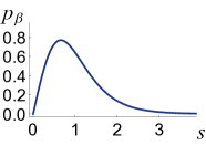
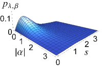
Figure 1: (Color online) Marginal probability distributions for (a) the subset of input squeezed states with arbitrary squeezing degree $s$ and arbitrary phase $\theta$, and (b) the complete set of input Gaussian states with arbitrary displacement $\alpha$, arbitrary squeezing degree $s$, and arbitrary random phase $\theta$. The plots show the marginal distributions after integrating over $\theta$, having set $\beta=2$, $\lambda=\frac{1}{2}$.

Case (a): Benchmark for arbitrary squeezed states.— We consider the ensemble $\Lambda_{S}$ of squeezed vacuum states $|\xi\rangle\equiv|\psi_{0,s,\theta}\rangle$ with arbitrary complex squeezing [see Eq. (1)] distributed according to the prior

$$p^{S}_{\beta}(\xi)=\frac{p_{\beta}(s)}{2\pi}\,,\quad\mbox{with}\ \ p_{\beta}(s)=\frac{\beta\sinh s}{(\cosh s)^{\beta+1}}\,,$$ (6)

where $\beta^{-1}>0$ regulates the width of the squeezing distribution, while the phase $\theta$ is uniformly distributed, which is natural for CV experiments Calsamiglia et al. (2009). The marginal prior $p_{\beta}(s)$ is plotted in Fig. 1(a). For squeezed states, the prior $p_{\beta}^{S}(\xi)$ is the analogue of the Gaussian $p_{\lambda}^{C}(\alpha)$ for coherent states: indeed, the Gaussian can be expressed as $p_{\lambda}^{C}(\alpha)\mathrm{d}^{2}\alpha=|\langle 0|\alpha\rangle|^{2\lambda}\mathrm{d}^{2}\alpha/\pi$, where the measure $\mathrm{d}^{2}\alpha$ is invariant under the action of displacements, while $p_{\beta}^{S}(\xi)$ can be expressed as $p_{\beta}^{S}(\xi)~{}\mathrm{d}s\mathrm{d}\theta=|\langle 0|\xi\rangle|^{2(2+\beta)}\mu(\mathrm{d}^{2}\xi)$, where the measure $\mu(\mathrm{d}^{2}\xi)=\sinh s\cosh s~{}\mathrm{d}s\mathrm{d}\theta/(2\pi)$ is invariant under the action of the squeezing transformations. For integer $\beta$, the prior $p_{\beta}^{S}(\xi)$ can be generated by preparing $2+\beta$ modes in the vacuum and performing the optimal measurement for the estimation of squeezing hay ; epa .

Using Eq. (5), the CFT can be written as $\overline{{\cal F}_{c}}^{S}(\beta)=\|A_{\beta}\|_{\times},\,A_{\beta}=(I\otimes\tau_{\beta}^{-1/2})\rho_{\beta}(I\otimes\tau_{\beta}^{-1/2})$ where $\tau_{\beta}=\int\mathrm{d}s\mathrm{d}\theta~{}p^{S}_{\beta}(\xi)|\xi\rangle\langle\xi|$ and $\rho_{\beta}=\int\mathrm{d}s\mathrm{d}\theta~{}p^{S}_{\beta}(\xi)~{}|\xi\rangle\langle\xi|\otimes|\xi\rangle\langle\xi|$. To obtain the benchmark announced in Eq. (3a), we compute explicitly the states $\tau_{\beta}$ and $\rho_{\beta}$ and show that the eigenvalues of $A_{\beta}$ are all equal to $\frac{1+\beta}{2+\beta}$ epa . Observing that $\frac{1+\beta}{2+\beta}=\langle 0|\langle 0|A_{\beta}|0\rangle|0\rangle$, we then get $\|A_{\beta}\|_{\times}=\frac{1+\beta}{2+\beta}$, thus concluding the proof of Eq. (3a). This benchmark allows one to certify the quantumness of experiments involving teleportation and storage of squeezed states with arbitrary amount of squeezing and arbitrary phase N. Takei et al. (2005); Yonezawa et al. (2007); K. Honda et al. (2008); Appel et al. (2008); K. Jensen et al. (2011), bypassing the limitations of Owari et al. (2008); Adesso and Chiribella (2008).

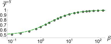
Figure 2: (Color online) Average classical fidelities for input squeezed states versus the distribution parameter $\beta$. The dots correspond to the fidelity $\overline{{\cal F}_{sr}}^{S}$ for the best square-root measurement, while the dashed line depicts the optimal probabilistic CFT $\overline{{\cal F}_{c}}^{S}$.

We highlight the similarity of our result to the case of input coherent states Hammerer et al. (2005). In that case, the probabilistic benchmark of Eq. (5) coincides with the maximum over deterministic strategies, given by Eq. (2) Chiribella and Xie (2013). Precisely, the CFT of Eq. (2) is achievable with heterodyne detection and repreparation of coherent states Braunstein et al. (2000); Hammerer et al. (2005). Since the heterodyne detection can be interpreted as a square-root measurement Hausladen and Wootters (1994); Hausladen et al. (1996) for a suitable Gaussian prior, in the case of squeezed states it is natural to wonder whether a deterministic square-root measurement strategy suffices to saturate the probabilistic CFT given by Eq. (3a). For an ensemble of the form $\{|\xi\rangle,p^{S}_{\eta}(\xi)\}$ the square-root measurement has POVM elements $P_{\eta}(\xi)=p^{S}_{\eta}(\xi)\tau_{\eta}^{-1/2}|\xi\rangle\langle\xi|\tau_{\eta}^{-1/2}$ (here we allow $\eta$ to be different from $\beta$). Performing the square-root measurement and repreparing the state $|\xi\rangle$ conditional on outcome $\xi$ gives the average fidelity $\overline{{\cal F}_{sr}}^{S}(\beta,\eta)=\frac{\beta}{\beta+2}\frac{\eta+1}{\eta+2}\sum_{k=0}^{\infty}{\left|\sum_{n=0}^{k}{k-n-\frac{1}{2}\choose k-n}\sqrt{{n-\frac{1}{2}\choose n}{\frac{\eta+1}{2}+n\choose n}}\right|^{2}}/\left[{{\frac{\beta+2}{2}+k\choose k}{\frac{\eta+2}{2}+k\choose k}}\right]$ epa , where we are using the notation ${x\choose k}=\frac{x(x-1)\dots(x-k+1)}{k!}$ for a general $x\in\mathbb{R}$. In Fig. 2 we compare $\sup_{\eta}\overline{{\cal F}_{sr}}^{S}(\beta,\eta)$, maximized numerically over $\eta$, with the CFT $\overline{{\cal F}_{c}}^{S}$ of Eq. (3a), for a range of values of $\beta$. We find that the square-root measurement is a nearly optimal classical strategy, which reaches the CFT asymptotically for large values of $\beta$, when the input squeezing distribution becomes more and more peaked.

Case (b): Benchmark for general Gaussian states.— Consider now the ensemble $\Lambda_{G}$ of arbitrary pure Gaussian states $|\alpha,\xi\rangle\equiv|\psi_{\alpha,s,\theta}\rangle$ [Eq. (1)] distributed according to the prior

$$p_{\lambda,\beta}^{G}(\alpha,s,\theta) = \frac{\lambda\beta}{2\pi^{2}}\frac{e^{-\lambda|\alpha|^{2}+\lambda{\rm Re}(e^{-i\theta}\alpha^{2})\tanh s}\sinh s}{(\cosh s)^{\beta+2}}\,.$$ (7)

We note that in this case the prior can be written as $p^{G}_{\lambda,\beta}(\xi)\propto|\langle 0|\lambda\alpha,\xi\rangle|^{2}|\langle 0|\xi\rangle|^{2(4+\beta)}\nu(\mathrm{d}^{2}\alpha,\mathrm{d}^{2}\xi)$ where $\nu(\mathrm{d}^{2}\alpha,\mathrm{d}^{2}\xi)=\mathrm{d}^{2}\alpha\sinh s(\cosh s)^{3}\mathrm{d}s\mathrm{d}\theta$ is the invariant measure under the joint action of displacement and squeezing. For integer $\beta$, the prior can be generated by performing an optimal measurement of squeezing and displacement on $5+\beta$ modes prepared in the vacuum epa . The marginals of this prior correctly reproduce the previous subcases, namely the distribution of Eq. (6) for the squeezing, $\int\mathrm{d}^{2}\alpha\ p^{G}_{\lambda,\beta}(\alpha,s,\theta)=p^{S}_{\beta}(\xi)$, and the Gaussian distribution of Hammerer et al. (2005) for the displacement, $\lim_{\beta\rightarrow\infty}\int\mathrm{d}^{2}\xi\ p^{G}_{\lambda,\beta}(\alpha,s,\theta)=p^{C}_{\lambda}(\alpha)$. The marginal probability distribution after integrating over the phase $\theta$, $p_{\lambda,\beta}(\alpha,s)=\int_{0}^{2\pi}\mathrm{d}\theta\ p^{G}_{\lambda,\beta}(\alpha,s,\theta)=\pi^{-1}\lambda\beta e^{-\lambda|\alpha|^{2}}\sinh s(\cosh s)^{-\beta-2}I_{0}\big{[}\lambda|\alpha|^{2}\tanh s\big{]}$, where $I_{0}$ is a modified Bessel function Abramowitz and Stegun (1964), is plotted in Fig. 1(b).

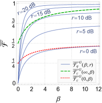
Figure 3: (Color online) Performance of the CV quantum teleportation protocol for general input Gaussian states $|\psi_{\alpha,s,\theta}\rangle$ using a two-mode squeezed entangled resource with squeezing $r$. (a) Plot of the quantum teleportation fidelity $\overline{{\cal F}_{q}}^{G}(\beta;r)$, averaged over the input set $\Lambda_{G}$ according to a prior distribution $p_{\lambda,\beta}$, against the benchmark $\overline{{\cal F}_{c}}^{G}(\lambda,\beta)$ for $\lambda\rightarrow 0$ (dotted red) and $\lambda\rightarrow\infty$ (dashed green). (b) Contour plot of $\overline{{\cal F}_{q}}^{G}(\beta;r)$ as a function of $\beta$ and $r$; the lower (red) and upper (green) shadings correspond to parameter regions where the quantum fidelity does not beat the benchmark $\overline{{\cal F}_{c}}^{G}(0,\beta)$ and $\overline{{\cal F}_{c}}^{G}(\infty,\beta)$, respectively.

To compute the benchmark, we observe that the pure Gaussian states of Eq. (1) are instances of the generalized coherent states introduced by Gilmore and Perelomov for arbitrary Lie groups Gilmore (1972); Perelomov (1972, 1986); Ali et al. (2000). Here we consider Gilmore-Perelomov coherent states of the form $|\varphi_{g}\rangle=\hat{U}_{g}|\varphi\rangle$, where $\hat{U}:g\mapsto\hat{U}_{g}$ is an irreducible representation of a Lie group $\mathsf{G}$ and $|\varphi\rangle$ is a lowest weight vector for the representation $\hat{U}:g\mapsto\hat{U}_{g}$. This general setting includes the cases of coherent and squeezed states, and the present case of pure Gaussian states, where the group is the Jacobi group, the group element $g$ is the pair $g=(\alpha,\xi)$, $\hat{U}_{g}\equiv\hat{D}(\alpha)\hat{S}(\xi)$, and $|\varphi\rangle\equiv|0\rangle$ Berceanu (2009). In the Supplemental Material epa , we solve the benchmark problem for arbitrary sets of Gilmore-Perelomov coherent states, randomly drawn with a prior probability of the form $p_{\gamma}(g)\mathrm{d}g\propto\,|\langle\varphi_{\gamma}|\varphi_{\gamma,g}\rangle|^{2}\,\mathrm{d}g$, where $\mathrm{d}g$ is the invariant measure on the group and $|\varphi_{\gamma,g}\rangle=\hat{U}^{\gamma}_{g}|\varphi_{\gamma}\rangle$ is the Gilmore-Perelomov coherent state for a given irreducible representation $\hat{U}^{\gamma}:g\mapsto\hat{U}_{g}^{\gamma}$. Our key result is a powerful formula for the probabilistic CFT for Gilmore-Perelomov coherent states, given by epa

$$\overline{{\cal F}_{c}}(\gamma)=\frac{\int\mathrm{d}g~{}p_{\gamma}(g)~{}|\langle\varphi|\varphi_{g}\rangle|^{4}}{\int\mathrm{d}g~{}p_{\gamma}(g)~{}|\langle\varphi|\varphi_{g}\rangle|^{2}}.$$ (8)

Using this general expression in the cases of coherent and squeezed states it is immediate to retrieve the benchmarks of Eqs. (2) and (3a). We now use this result to find the benchmark for the transmission of arbitrary input Gaussian states with prior distribution given by Eq. (7), which now reads

$$\overline{{\cal F}_{c}}^{G}(\lambda,\beta)=\frac{\int\mathrm{d}^{2}\alpha\,\mathrm{d}s\,\mathrm{d}\theta\ p^{G}_{\lambda,\beta}(\alpha,s,\theta)|\langle 0|\psi_{\alpha,s,\theta}\rangle|^{4}}{\int\mathrm{d}^{2}\alpha\,\mathrm{d}s\,\mathrm{d}\theta\ p^{G}_{\lambda,\beta}(\alpha,s,\theta)|\langle 0|\psi_{\alpha,s,\theta}\rangle|^{2}}\,.$$ (9)

The integrals can be evaluated analytically epa . The final result yields the general benchmark announced in Eq. (3b), which is the main contribution of this Letter. Notice how the previous partial findings are contained in this result. For coherent states, $\lim_{\beta\rightarrow\infty}\overline{{\cal F}_{c}}^{G}(\lambda,\beta)=\overline{{\cal F}_{c}}^{C}(\lambda)$; for squeezed states, $\lim_{\lambda\rightarrow\infty}\overline{{\cal F}_{c}}^{G}(\lambda,\beta)=\overline{{\cal F}_{c}}^{S}(\beta)$. The benchmark for teleporting Gaussian states in the limit of completely random $\alpha,s,\theta$ is finally established to be $\lim_{\lambda,\beta\rightarrow 0}\overline{{\cal F}_{c}}^{G}(\lambda,\beta)=\frac{1}{4}$.

Discussion.— We now investigate how well an actual implementation of quantum teleportation can fare against the benchmarks derived above. We focus on the conventional Braunstein–Kimble CV quantum teleportation protocol Braunstein and Kimble (1998) using as a resource a Gaussian two-mode squeezed vacuum state with squeezing $r$, $|\phi\rangle_{AB}=(\cosh r)^{-1}\sum_{k=0}^{\infty}(\tanh r)^{k}|k\rangle_{A}|k\rangle_{B}$, also known as a twin-beam. We assume that the input is an arbitrary pure single-mode Gaussian state $|\psi_{\alpha,s,\theta}\rangle$, Eq. (1), drawn according to the probability distribution of Eq. (7). The output state received by Bob will be a Gaussian mixed state whose fidelity with the input can be written as Adesso and Chiribella (2008) ${\cal F}_{q}(s;r)=\{2e^{-2r}[\cosh(2r)+\cosh(2s)]\}^{-\frac{1}{2}}$. Notice that it depends neither on the phase $\theta$ nor the displacement $\alpha$ by construction of the CV protocol Braunstein and Kimble (1998) (for unit gain van Loock (2002); Furusawa and Takei (2007)). Averaging this over the input set $\Lambda_{G}$ we get the average quantum teleportation fidelity

$$\overline{{\cal F}_{q}}^{G}(\beta;r) = \begin{array}[]{c}\int\mathrm{d}\theta\,\mathrm{d}^{2}\alpha\,\mathrm{d}s\ p^{G}_{\lambda,\beta}(\alpha,s,\theta){\cal F}_{q}(s;r)\end{array}$$ (11)

$$= \begin{array}[]{c}\frac{\beta}{2\beta+2}e^{r}\ _{2}F_{1}\left(\frac{1}{2},\frac{\beta+1}{2};\frac{\beta+3}{2};-\sinh^{2}(r)\right)\end{array},$$ (13)

where ${}_{2}F_{1}$ is a hypergeometric function Abramowitz and Stegun (1964). The average quantum fidelity is obviously independent of $\lambda$, i.e., in particular, it is the same for the ensemble of all Gaussian states $\Lambda_{G}$ and for the ensemble of squeezed states $\Lambda_{S}$. In Fig. 3, we compare $\overline{{\cal F}_{q}}^{G}(\beta;r)$ with the CFT $\overline{{\cal F}_{c}}^{G}(\lambda,\beta)$, in particular with the case $\lambda\rightarrow 0$ (totally random displacement) and with the case $\lambda\rightarrow\infty$ (undisplaced squeezed states, whose CFT reduces to $\overline{{\cal F}_{c}}^{S}(\beta)$). In the latter case, we see that the shared entangled state needs to have a squeezing $r$ above $10$ dB, which is at the edge of current technology T. Eberle et al. (2010); Eberle et al. (2013), in order to beat the benchmark for the ensemble $\Lambda_{S}$. For general input Gaussian states in $\Lambda_{G}$ with random displacement, squeezing, and phase, less resources are instead needed to surpass the CFT of Eq. (3b), especially if the input squeezing distribution is not too broad ($\beta\gg 0$), which is the realistic situation in experimental implementations (where e.g. $s$ can fluctuate around a set value which depends on the specifics of the nonlinear crystal used for optical parametric amplification Cerf et al. (2007); Furusawa and Takei (2007)). For the case of coherent input states with totally random displacement ($\lambda\rightarrow 0,\beta\rightarrow\infty$), the CFT converges to $\frac{1}{2}$ and we recover the known result that any $r>0$ is enough to beat the corresponding benchmark Braunstein and Kimble (1998); Braunstein et al. (2000); Furusawa et al. (1998); Hammerer et al. (2005); Adesso and Illuminati (2005).

Summarizing, we have derived exact analytical quantum benchmarks for teleportation and storage of arbitrary pure single-mode Gaussian states, which can be readily employed to validate current and future implementations. The mathematical techniques developed here to obtain the presented results are of immediate usefulness to analyze a much larger class of problems, such as the determination of benchmarks for cloning, amplification Chiribella and Xie (2013) and other protocols involving multimode Gaussian states and other classes of Gilmore-Perelomov coherent states, including finite-dimensional states. We will explore these topics in forthcoming publications.

Acknowledgments.—This work was supported by the Tsinghua–Nottingham Teaching and Research Fund. GC is supported by the National Basic Research Program of China (973) 2011CBA00300 (2011CBA00301), by the National Natural Science Foundation of China (Grants 11350110207, 61033001, 61061130540), and by the 1000 Youth Fellowship Program of China. GC thanks S. Berceanu for useful discussions on the Jacobi group. GA thanks N. G. de Almeida for discussions and the Brazilian agency CAPES (Pesquisador Visitante Especial-Grant No. 108/2012) for financial support.

Supplemental Material: Quantum benchmarks for pure single-mode Gaussian states

Appendix A Proof of Eq. (3a): benchmark for squeezed vacuum states

Let us expand the squeezed states as

$$|\xi\rangle :=e^{\frac{1}{2}(\xi\hat{a}^{{\dagger}2}-\xi^{\ast}\hat{a}^{2})}|0\rangle$$

$$=\frac{1}{\sqrt{\cosh s}}\sum_{n=0}^{\infty}\sqrt{n-\frac{1}{2}\choose n}\left({\tanh s}\right)^{n}e^{in\theta}|2n\rangle\,,\qquad\xi=se^{i\theta}$$

using the notation ${x\choose n}:=\frac{x(x-1)\dots(x-n+1)}{n!}$ for a generic $x\in\mathbb{R}$. We now compute the average states of the ensembles $\left\{|\xi\rangle,p^{S}_{\beta}(\xi)\right\}$ and $\left\{|\xi\rangle\otimes|\xi\rangle,p^{S}_{\beta}(\xi)\right\}$, where $p^{S}_{\beta}(\xi)$ is the probability distribution

$$p^{S}_{\beta}(\xi)=\frac{\beta\sinh s~{}}{(\cosh s)^{\beta+1}}~{}\frac{~{}1}{2\pi}\,,\qquad\beta>0,$$

satisfying the normalization condition $\int\mathrm{d}s\mathrm{d}\theta~{}p_{\beta}^{S}(\xi)=1$. By explicit calculation, we find that the average states are

$$\tau_{\beta}:=\int\mathrm{d}s\mathrm{d}\theta~{}p^{S}_{\beta}(\xi)~{}|\xi\rangle\langle\xi|=\frac{\beta}{\beta+1}\sum_{n=0}^{\infty}\frac{{n-\frac{1}{2}\choose n}}{{\frac{\beta+1}{2}+n\choose n}}~{}|2n\rangle\langle 2n|,$$ (14)

and

$$\rho_{\beta}:= \int\mathrm{d}s\mathrm{d}\theta~{}p^{S}_{\beta}(\xi)~{}|\xi\rangle\langle\xi|\otimes|\xi\rangle\langle\xi|=\frac{\beta}{\beta+2}\sum_{k=0}^{\infty}\frac{1}{{\frac{\beta+2}{2}+k\choose k}}|\Phi_{k}\rangle\langle\Phi_{k}|$$ (15)

where

$$|\Phi_{k}\rangle :=\sum_{n=0}^{k}\sqrt{{k-n-\frac{1}{2}\choose k-n}{n-\frac{1}{2}\choose n}}~{}|2k-2n\rangle|2n\rangle.$$ (16)

Now, by Ref. S (1) the probabilistic CFT is given by

$$\overline{{\cal F}_{c}}^{S}(\beta)=\left\|A_{\beta}\right\|_{\times}\,,\qquad A_{\beta}:=\left(I\otimes\tau_{\beta}^{-1/2}\right)\rho_{\beta}\left(I\otimes\tau_{\beta}^{-1/2}\right)\,,$$

where $\|A_{\beta}\|_{\times}$ is the cross norm of $A_{\beta}$, defined as $\left\|A_{\beta}\right\|_{\times}:=\sup_{\|\varphi\|=\|\psi\|=1}\langle\varphi|\langle\psi|A_{\beta}|\varphi\rangle|\psi\rangle$. Using Eq. (15), one can write the operator $A_{\beta}$ as

$$A_{\beta}=\frac{\beta}{\beta+2}\sum_{k=0}^{\infty}\frac{1}{{\frac{\beta+2}{2}+k\choose k}}~{}\left(I\otimes\tau_{\beta}^{-\frac{1}{2}}\right)|\Phi_{k}\rangle\langle\Phi_{k}|\left(I\otimes\tau_{\beta}^{-\frac{1}{2}}\right)$$

where the vectors $\left(I\otimes\tau_{\beta}^{-\frac{1}{2}}\right)|\Phi_{k}\rangle$ are mutually orthogonal for different values of $k$, as can be seen by direct inspection using Eq. (14). Using this fact, one can compute the eigenvalues of $A_{\beta}$, which are given by

$$a_{\beta,k} =\frac{\beta}{\beta+2}\frac{1}{{\frac{\beta+2}{2}+k\choose k}}\langle\Phi_{k}|(I\otimes\tau_{\beta}^{-1})|\Phi_{k}\rangle$$

$$=\frac{\beta+1}{\beta+2}\frac{1}{{\frac{\beta+2}{2}+k\choose k}}\sum_{n=0}^{k}{k-n-\frac{1}{2}\choose k-n}{\frac{\beta+1}{2}+n\choose n}$$

$$=\frac{\beta+1}{\beta+2}\frac{(-1)^{k}}{{\frac{\beta+2}{2}+k\choose k}}\sum_{n=0}^{k}{-\frac{1}{2}\choose k-n}{-\frac{\beta+3}{2}\choose n}$$

$$=\frac{\beta+1}{\beta+2}~{}\frac{(-1)^{k}}{{\frac{\beta+2}{2}+k\choose k}}{-\frac{\beta+4}{2}\choose k}$$

$$=\frac{\beta+1}{\beta+2},$$

(the fourth equality coming from the Chu-Vandermonde identity S (2)). In other words, $A_{\beta}$ is proportional to a projector, with the proportionality constant $(\beta+1)/(\beta+2)$. This proves that

$$\left\|A_{\beta}\right\|_{\times} =\sup_{\|\varphi\|=\|\psi\|=1}\langle\varphi|\langle\psi|A_{\beta}|\varphi\rangle|\psi\rangle$$

$$\leq\frac{\beta+1}{\beta+2}.$$

On the other hand, observing that $\langle 0|\langle 0|A_{\beta}|0\rangle|0\rangle=\frac{\beta+1}{\beta+2}$ we conclude that

$$\overline{{\cal F}_{c}}^{S}(\beta)=\left\|A_{\beta}\right\|_{\times}=\frac{\beta+1}{\beta+2}.$$

Appendix B The fidelity of the square-root measurement

For the the ensemble of squeezed states $\{|\xi\rangle,p^{S}_{\eta}(\mathrm{d}^{2}\xi)\}$ the square-root measurement is the POVM with operators $P_{\eta}(\xi)=p^{S}_{\eta}(\xi)\tau_{\eta}^{-\frac{1}{2}}|\xi\rangle\langle\xi|\tau_{\eta}^{-\frac{1}{2}}$ S (3, 4). Hence, the fidelity of the measure-and-prepare protocol based on measuring the square-root measurement and on re-preparing squeezed states is given by

$$\overline{F_{sr}}^{S} =\int\mathrm{d}s\mathrm{d}\theta\int\mathrm{d}s^{\prime}\mathrm{d}\theta^{\prime}~{}p_{\beta}^{S}(\xi)~{}|\langle\xi|\xi^{\prime}\rangle|^{2}~{}\langle\xi|P_{\eta}(\xi^{\prime})|\xi\rangle$$

$$=\int\mathrm{d}s\mathrm{d}\theta\int\mathrm{d}s^{\prime}\mathrm{d}\theta^{\prime}~{}p_{\beta}^{S}(\xi)p_{\beta}^{S}(\xi^{\prime})~{}\mathrm{Tr}\left[\left(|\xi\rangle\langle\xi|^{\phantom{\frac{1}{2}}}_{\phantom{\eta}}\otimes|\xi\rangle\langle\xi|\right)\left(|\xi^{\prime}\rangle\langle\xi^{\prime}|\otimes\tau_{\eta}^{-\frac{1}{2}}|\xi^{\prime}\rangle\langle\xi^{\prime}|\tau_{\eta}^{-\frac{1}{2}}\right)\right]$$

$$=\mathrm{Tr}\left[\rho_{\beta}(I\otimes\tau_{\eta}^{-\frac{1}{2}})\rho_{\eta}(I\otimes\tau_{\eta}^{-\frac{1}{2}})\right]\,.$$

Inserting Eqs.  (14), (15), and (16) into the last equation we then obtain

$$\overline{F_{sr}}^{S} =\frac{\beta}{\beta+2}\frac{\eta}{\eta+2}\sum_{k=0}^{\infty}\frac{1}{{\frac{\beta+2}{2}+k\choose k}{\frac{\eta+2}{2}+k\choose k}}\left|\langle\Phi_{k}|\left(I\otimes\tau_{\eta}^{-\frac{1}{2}}\right)|\Phi_{k}\rangle\right|^{2}$$

$$=\frac{\beta}{\beta+2}\frac{\eta+1}{\eta+2}\sum_{k=0}^{\infty}\frac{1}{{\frac{\beta+2}{2}+k\choose k}{\frac{\eta+2}{2}+k\choose k}}{\left|\sum_{n=0}^{k}{k-n-\frac{1}{2}\choose k-n}\sqrt{{n-\frac{1}{2}\choose n}{\frac{\eta+1}{2}+n\choose n}}\right|^{2}}\,,$$

which is the expression used in the main text.

Appendix C Proof of Eq. (8): benchmark for teleportation and storage of Gilmore-Perelomov coherent states

Consider a generic Lie group ${\mathbf{G}}$, acting on a Hilbert space $\mathcal{H}$ through a unitary irreducible representation $\hat{U}:g\mapsto\hat{U}_{g}$. In the following we refer to the monographies S (5, 6) for the background on coherent states and representation theory. We will consider Gilmore-Perelomov coherent states S (7, 8) and $|\varphi_{g}\rangle$ of the form $|\varphi_{g}\rangle=\hat{U}_{g}|\varphi\rangle$, where $|\varphi\rangle$ is a lowest weight vector for the representation $U$, i.e. a vector that is annihilated by all the negative roots of the Lie algebra Examples of Gilmore-Perelomov coherent states are the ordinary coherent states $|\alpha\rangle=\hat{D}(\alpha)|0\rangle$, associated to the Weyl-Heisenberg group, the squeezed states $|\xi\rangle=\hat{S}(\xi)|0\rangle$, associated to the group $SU(1,1)$, and the displaced squeezed states $|\alpha,\xi\rangle=\hat{D}(\alpha)\hat{S}(\xi)|0\rangle$, associated to the Jacobi group. Other examples, in finite dimensional quantum systems, are the pure states $|\varphi_{U}\rangle=U|\varphi_{0}\rangle$, $U\in SU(d)$ and the spin-coherent states $|j,j,\varphi,\vec{n}\rangle=R^{(j)}_{\varphi,\vec{n}}|j,j\rangle$ associated to the rotation group $SO(3)$.

We now prove a general formula to compute the classical fidelity threshold for the teleportation and storage of Gilmore-Perelomov coherent states. Among the possible measure-and-prepare strategies, we include probabilistic strategies based on abstention. To stress this fact, we refer to our CFT as probabilistic CFT. We assume that the group is unimodular—that is, it has a left- and right- invariant measure $\mathrm{d}g$—, and that the input state $|\varphi_{g}\rangle$ is given with prior probability

$$p_{\gamma}(\mathrm{d}g)=d_{\gamma}|\langle\varphi_{\gamma}|\varphi_{\gamma,g}\rangle|^{2}\mathrm{d}g,$$ (17)

where $|\varphi_{\gamma,g}\rangle:=\hat{U}^{\gamma}_{g}|\varphi_{\gamma}\rangle\in\mathcal{H}_{\gamma}$ is a coherent state for some other irreducible representation $\hat{U}^{\gamma}:g\to\hat{U}^{\gamma}_{g}$ and $d_{\gamma}$ is a normalization constant, known as formal dimension, given by

$$d_{\gamma}:=\left(\int\mathrm{d}g~{}|\langle\varphi_{\gamma}|\varphi_{\gamma,g}\rangle|^{2}\right)^{-1}.$$ (18)

Of course, in order for the probability distribution $p_{\gamma}(\mathrm{d}g)$ to be normalizable, the formal dimension $d_{\gamma}$ should not be zero (i.e. the integral in Eq. (18) should not diverge). Technically, irreducible representations with this property are called square-summable. Since we want $p_{\gamma}^{S}(\mathrm{d}g)$ to be a probability distribution, in the following we will always assume that the representation $\hat{U}_{\gamma}$ is square-summable.

In addition, we will always assume that that the root system that makes $|\varphi_{\gamma}\rangle$ a lowest weight vector has been chosen to have the same structure constants of the root system that makes $|\varphi\rangle$ a lowest weight vector. For example, this is what is done in quantum optics when one has two annihilation operators $\hat{a}$ and $\hat{b}$ for two different modes $A$ and $B$, that are chosen in such a way that $[\hat{a},\hat{a}^{\dagger}]=I_{A}$ and $[\hat{b},\hat{b}^{\dagger}]=I_{B}$. With this choice, the negative roots of the Lie algebra representation associated to the product representations $\hat{U}\otimes\hat{U}_{\gamma}$ and $\hat{U}\otimes\hat{U}\otimes\hat{U}_{\gamma}$ will be the sum of the negative roots of the Lie algebra representation associated to $\hat{U}$ and $\hat{U}_{\gamma}$. Hence, the fact that both $|\varphi\rangle$ and $|\varphi_{\gamma}\rangle$ are annihilated by the negative roots, implies that also the states $|\varphi\rangle|\varphi_{\gamma}\rangle$ and $|\varphi\rangle|\varphi\rangle|\varphi_{\gamma}\rangle$ are annihilated by the negative roots, i.e. they are lowest weight vectors. In the example of quantum optics, this corresponds to the fact that product of the vacuum states for two modes $a$ and $b$ is the vacuum state for the mode $a+b$. Our choice of root system guarantees also that the product representations $\hat{U}\otimes\hat{U}_{\gamma}$ and $\hat{U}\otimes\hat{U}\otimes\hat{U}_{\gamma}$ are square summable: indeed, one has

$$d_{\hat{U}\otimes\hat{U}\otimes\hat{U}_{\gamma}} \equiv\left(\int\mathrm{d}g~{}|\langle\varphi|\varphi_{g}\rangle|^{4}|\langle\varphi_{\gamma}|\varphi_{\gamma,g}\rangle|^{2}\right)^{-1}$$

$$\geq\left(\int\mathrm{d}g~{}|\langle\varphi|\varphi_{g}\rangle|^{2}|\langle\varphi_{\gamma}|\varphi_{\gamma,g}\rangle|^{2}\right)^{-1}$$

$$\equiv d_{\hat{U}\otimes\hat{U}_{\gamma}}$$

$$\geq\left(\int\mathrm{d}g~{}|\langle\varphi_{\gamma}|\varphi_{\gamma,g}\rangle|^{2}\right)^{-1}$$

$$\equiv d_{\gamma}$$

$$>0\,.$$

With the above settings, we have the following result

Theorem 1 (Benchmark for Gilmore-Perelomov coherent states)

Let $\Lambda=\{|\varphi_{g}\rangle,p_{\gamma}(\mathrm{d}g)\}_{g\in{\mathbf{G}}}$ be an ensemble of Gilmore-Perelomov coherent states, with prior probability distribution of the form $p_{\gamma}(\mathrm{d}g)=d_{\gamma}|\langle\varphi_{\gamma}|\varphi_{\gamma,g}\rangle|^{2}\mathrm{d}g$. Then, the probabilistic CFT is

$$\overline{{\cal F}_{c}}(\gamma)=\frac{\int\mathrm{d}g~{}p_{\gamma}(g)|\langle\varphi|\varphi_{g}\rangle|^{4}}{\int\mathrm{d}g~{}p_{\gamma}(g)|\langle\varphi|\varphi_{g}\rangle|^{2}}.$$ (19)

Proof. By the result of Ref. S (1), the CFT is given by the cross norm

$$\overline{{\cal F}_{c}}(\gamma) =\left\|A_{\gamma}\right\|_{\times}\qquad\left\{\begin{array}[]{ll}A_{\gamma}&:=(I\otimes\tau_{\gamma}^{-1/2})\rho_{\gamma}(I\otimes\tau_{\gamma}^{-1/2})\\ \tau_{\gamma}&:=\int\mathrm{d}g~{}p_{\gamma}(g)~{}|\varphi_{g}\rangle\langle\varphi_{g}|\\ \rho_{\gamma}&:=\int\mathrm{d}g~{}p_{\gamma}(g)~{}|\varphi_{g}\rangle\langle\varphi_{g}|\otimes|\varphi_{g}\rangle\langle\varphi_{g}|\end{array}\right.$$

$$\leq\|A_{\gamma}\|_{\infty}$$

$$=\min\{\lambda\geq 0~{}|~{}\lambda(I\otimes\tau_{\gamma})\geq\rho_{\gamma}\}$$

Now, using Eq. (17), we have

$$\tau_{\gamma} =d_{\gamma}\mathrm{Tr}_{\gamma}\left[\left(\int\mathrm{d}g~{}|\varphi_{g}\rangle\langle\varphi_{g}|\otimes|\varphi_{\gamma,g}\rangle\langle\varphi_{\gamma,g}|\right)(I\otimes|\varphi_{\gamma}\rangle\langle\varphi_{\gamma}|)\right]$$ (20)

$$\rho_{\gamma} =d_{\gamma}\mathrm{Tr}_{\gamma}\left[\left(\int\mathrm{d}g~{}|\varphi_{g}\rangle\langle\varphi_{g}|\otimes|\varphi_{g}\rangle\langle\varphi_{g}|\otimes|\varphi_{\gamma,g}\rangle\langle\varphi_{\gamma,g}|\right)\left(I\otimes I\otimes|\varphi_{\gamma}\rangle\langle\varphi_{\gamma}|\right)\right]\,,$$ (21)

where $\mathrm{Tr}_{\gamma}$ is a shorthand notation for the partial trace over the Hilbert space $\mathcal{H}_{\gamma}$. Now, since the state $|\varphi\rangle|\varphi_{\gamma}\rangle$ (respectively, $|\varphi\rangle|\varphi\rangle|\varphi_{\gamma}\rangle$) is a lowest weight vector, the states $|\varphi_{g}\rangle|\varphi_{\gamma,g}\rangle$ (respectively, $|\varphi_{g}\rangle|\varphi_{g}\rangle|\varphi_{\gamma,g}\rangle$) belong to a single irreducible subspace, denoted by $\mathcal{H}_{\gamma_{1}}$ (respectively, $\mathcal{H}_{2}$). Precisely, they belong to the irreducible subspace that carries the Cartan component of $\hat{U}\otimes\hat{U}^{\gamma}$ (respectively, $\hat{U}\otimes\hat{U}\otimes\hat{U}^{\gamma}$). By Schur’s lemma the integral in the r.h.s. of both equations (20) is proportional to a projector, namely

$$\tau_{\gamma} =d_{\gamma}\mathrm{Tr}_{\gamma}\left[\frac{\hat{P}_{\gamma_{1}}}{d_{\gamma_{1}}}\left(I\otimes|\varphi_{\gamma}\rangle\langle\varphi_{\gamma}|\right)\right]$$ (22)

$$\rho_{\gamma} =d_{\gamma}\mathrm{Tr}_{\gamma}\left[\frac{\hat{P}_{\gamma_{2}}}{d_{\gamma_{2}}}\left(I\otimes I\otimes|\varphi_{\gamma}\rangle\langle\varphi_{\gamma}|\right)\right]$$ (23)

where $\hat{P}_{\gamma_{1}}$ ($\hat{P}_{\gamma_{2}}$) is the projector on $\mathcal{H}_{\gamma_{1}}$ ($\mathcal{H}_{\gamma_{2}}$) and $d_{\gamma_{1}}$ ($d_{\gamma_{2}}$) is the formal dimension of the Cartan component of $\hat{U}\otimes\hat{U}^{\gamma}$ ($\hat{U}\otimes\hat{U}\otimes\hat{U}^{\gamma}$). Clearly, choosing $\lambda=d_{\gamma_{2}}/d_{\gamma_{2}}$, we have $\lambda\left(I\otimes\frac{\hat{P}_{\gamma_{1}}}{d_{\gamma_{1}}}\right)\geq\frac{\hat{P}_{\gamma_{2}}}{d_{\gamma_{2}}}$, and, by Eqs. (22) and (23), $\lambda(I\otimes\tau_{\gamma})\geq\rho_{\gamma}$. Hence, we conclude that $\overline{{\cal F}_{c}}(\gamma)\leq d_{\gamma_{1}}/d_{\gamma_{2}}$.

On the other hand, the upper bound can be achieved. First of all, note that $|\varphi\rangle$ is an eigenvector of $\tau_{\gamma}$: indeed, using Eq. (22) one has

$$\tau_{\gamma}|\varphi\rangle=d_{\gamma}\mathrm{Tr}_{\gamma}\left[\frac{\hat{P}_{\gamma_{1}}}{d_{\gamma_{1}}}\left(I\otimes|\varphi_{\gamma}\rangle\langle\varphi_{\gamma}|\right)\right]|\varphi\rangle=\frac{d_{\gamma}}{d_{\gamma_{1}}}|\varphi\rangle.$$

Similarly, $|\varphi\rangle|\varphi\rangle$ is an eigenvector of $\rho_{\gamma}$: using Eq. (23) one has

$$\rho_{\gamma}|\varphi\rangle|\varphi\rangle=d_{\gamma}\mathrm{Tr}_{\gamma}\left[\frac{\hat{P}_{\gamma_{2}}}{d_{\gamma_{2}}}\left(I\otimes I\otimes|\varphi_{\gamma}\rangle\langle\varphi_{\gamma}|\right)\right]|\varphi\rangle|\varphi\rangle=\frac{d_{\gamma}}{d_{\gamma_{2}}}|\varphi\rangle|\varphi\rangle.$$

Hence, we obtain

$$\overline{{\cal F}_{c}}(\gamma) =\left\|(I_{\otimes}\tau_{\gamma}^{-1/2})\rho_{\gamma}(I\otimes\tau_{\gamma}^{-1/2})\right\|_{\times}$$

$$\geq\langle\varphi|\langle\varphi|(I\otimes\tau_{\gamma}^{-1/2})\rho_{\gamma}(I\otimes\tau_{\gamma}^{-1/2})|\varphi\rangle|\varphi\rangle$$

$$=\frac{d_{\gamma_{2}}}{d_{\gamma_{2}}}.$$

Combining the upper and lower bounds we obtain $\overline{{\cal F}_{c}}(\gamma)={d_{\gamma_{1}}}/{d_{\gamma_{2}}}$. Using Eq. (18) for the evaluation of $d_{\gamma_{1}}$ and $d_{\gamma_{2}}$ concludes the proof. $\,\blacksquare$

Using Eq. (19) it is immediate to recover the benchmarks for coherent states and for squeezed states: indeed, one has

$$\frac{\int\mathrm{d}^{2}\alpha/\pi~{}\lambda e^{-\lambda|\alpha|^{2}}~{}|\langle 0|\alpha\rangle|^{4}}{\int\mathrm{d}^{2}\alpha/\pi~{}\lambda e^{-\lambda|\alpha|^{2}}~{}|\langle 0|\alpha\rangle|^{2}}=\frac{1+\lambda}{2+\lambda}=\overline{{\cal F}_{c}}^{C}(\lambda)$$ (24)

and

$$\frac{\int\mathrm{d}s\mathrm{d}\theta/2\pi~{}[\beta\sinh s/(\cosh s)^{1+\beta}]~{}|\langle 0|\xi\rangle|^{4}}{\int\mathrm{d}s\mathrm{d}\theta/2\pi~{}[\beta\sinh s/(\cosh s)^{1+\beta}]~{}|\langle 0|\xi\rangle|^{2}}=\frac{1+\beta}{2+\beta}=\overline{{\cal F}_{c}}^{S}(\beta).$$ (25)

Note that for squeezed states the group-theoretical argument of Theorem 1 guarantees optimality only for integer $\beta$ (the square-summable irreducible representations of $SU(1,1)$ form a discrete set), while the optimality proof for general real-valued positive $\beta$ requires the explicit argument presented in section A.

Appendix D Proof of Eq. (3b): benchmark for general pure Gaussian states

Pure Gaussian states can be parameterized as

$$|\alpha,\xi\rangle :=\hat{D}(\alpha)\hat{S}(\xi)|0\rangle\,,\qquad\xi=se^{i\theta}.$$

Here the displacement and squeezing operators generate a representation of the Jacobi group, and the vacuum is a lowest weight vector for this representation S (9). Note that the overlap between one pure Gaussian state and the vacuum is

$$|\langle 0|\alpha,\xi\rangle|^{2}=\frac{e^{-|\alpha|^{2}+{\rm Re}(e^{-i\theta}\alpha^{2})\tanh s}}{\cosh s}$$ (26)

For the probability distribution, we choose

$$p^{G}_{\lambda,\beta}(\alpha,s,\theta)~{}\mathrm{d}^{2}\alpha\mathrm{d}s\mathrm{d}\theta\propto|\langle 0|\lambda\alpha,\xi\rangle|^{2}~{}|\langle 0|\xi\rangle|^{2(4+\beta)}~{}\nu(\mathrm{d}^{2}\alpha,\mathrm{d}^{2}\xi),$$

where $\nu(\mathrm{d}^{2}\alpha,\mathrm{d}^{2}\xi)=\mathrm{d}^{2}\alpha\sinh s(\cosh s)^{3}\mathrm{d}s\mathrm{d}\theta$ is the invariant measure over the Jacobi group. Using Eq. (26), we can write down the explicit expression

$$p_{\lambda,\beta}^{G}(\alpha,s,\theta) = \frac{\lambda\beta}{2\pi^{2}}\frac{e^{-\lambda|\alpha|^{2}+\lambda\tanh s{\rm Re}(e^{-i\theta}\alpha^{2})}\sinh s}{(\cosh s)^{\beta+2}}.$$

For integer $\beta$, the states $|\lambda\alpha,\xi\rangle|\xi\rangle^{\otimes{4+\beta}}$ are Gilmore-Perelomov coherent states generated by the action of the representation $\hat{D}(\lambda\alpha)\hat{S}(\xi)\otimes\hat{S}(\xi)^{\otimes 4+\beta}$ on the lowest weight vector $|0\rangle|0\rangle^{\otimes(4+\beta)}$. Hence, using Eq. (19) we can compute the probabilistic CFT as

$$\overline{{\cal F}_{c}}^{G}(\lambda,\beta) =\frac{\int\mathrm{d}^{2}\alpha\,\mathrm{d}s\,\mathrm{d}\theta\ p^{G}_{\lambda,\beta}(\alpha,s,\theta)|\langle 0|\psi_{\alpha,s,\theta}\rangle|^{4}}{\int\mathrm{d}^{2}\alpha\,\mathrm{d}s\,\mathrm{d}\theta\ p^{G}_{\lambda,\beta}(\alpha,s,\theta)|\langle 0|\psi_{\alpha,s,\theta}\rangle|^{2}}$$

$$=\frac{\int\mathrm{d}^{2}\alpha\,\mathrm{d}s\,\mathrm{d}\theta\ e^{-(2+\lambda)\left[|\alpha|^{2}+{\rm Re}(e^{-i\theta}\alpha^{2})\tanh s\right]}~{}\sinh s(\cosh s)^{-4-\beta}}{\int\mathrm{d}^{2}\alpha\,\mathrm{d}s\,\mathrm{d}\theta\ e^{-(1+\lambda)\left[|\alpha|^{2}+{\rm Re}(e^{-i\theta}\alpha^{2})\tanh s\right]}~{}\sinh s(\cosh s)^{-3-\beta}}$$

$$=\frac{\int\mathrm{d}^{2}\alpha\,\mathrm{d}s\ e^{-(2+\lambda)\left|\alpha\right|^{2}}\sinh s(\cosh s)^{-4-\beta}I_{0}\left((2+\lambda)\left|\alpha\right|^{2}\tanh s\right)}{\int\mathrm{d}^{2}\alpha\,\mathrm{d}s\ e^{-(1+\lambda)\left|\alpha\right|^{2}}\sinh s(\cosh s)^{-3-\beta}I_{0}\left((1+\lambda)\left|\alpha\right|^{2}\tanh s\right)}$$

$$=\left(\frac{1+\lambda}{2+\lambda}\right)\frac{\int\mathrm{d}s\ \sinh s(\cosh s)^{-3-\beta}}{\int\mathrm{d}s\ \sinh s(\cosh s)^{-2-\beta}}$$

$$=\frac{(1+\lambda)(1+\beta)}{(2+\lambda)(2+\beta)}\,.$$

For general noninteger positive $\beta$ we prove the optimality of the value $\frac{(1+\lambda)(1+\beta)}{(2+\lambda)(2+\beta)}$ directly from the expression of Ref. S (1), which in this case reads

$$\overline{{\cal F}_{c}}^{G}(\lambda,\beta) =\left\|A_{\lambda,\beta}\right\|_{\times}\qquad\left\{\begin{array}[]{ll}A_{\lambda,\beta}&:=(I\otimes\tau_{\lambda,\beta}^{-1/2})\rho_{\lambda,\beta}(I\otimes\tau_{\lambda,\beta}^{-1/2})\\ \tau_{\lambda,\beta}&:=\int\mathrm{d}^{2}\alpha\mathrm{d}s\mathrm{d}\theta~{}p_{\lambda,\beta}(\alpha,s,\theta)~{}|\alpha,s,\theta\rangle\langle\alpha,s,\theta|\\ \rho_{\lambda,\beta}&:=\int\mathrm{d}^{2}\alpha\mathrm{d}s\mathrm{d}\theta~{}p_{\lambda,\beta}(\alpha,s,\theta)~{}|\alpha,s,\theta\rangle\langle\alpha,s,\theta|\otimes|\alpha,s,\theta\rangle\langle\alpha,s,\theta|\end{array}\right.$$

In order to show that $\left\|A_{\lambda,\beta}\right\|_{\times}=\frac{(1+\lambda)(1+\beta)}{(2+\lambda)(2+\beta)}$, we observe that, by the symmetry of the prior distribution, the average state $\tau_{\lambda,\beta}$ commutes with the phase shifts $\hat{U}_{\varphi}=e^{i\varphi\hat{a}^{\dagger}a}$, and, therefore, it is diagonal on the Fock basis. Hence, we can write it as

$$\tau_{\lambda,\beta}=\sum_{n=0}^{\infty}t_{n}|n\rangle\langle n|\,,~{}\qquad t_{n}=\int\mathrm{d}^{2}\alpha~{}\mathrm{d}s~{}\mathrm{d}\theta~{}p_{\lambda,\beta}^{G}(\alpha,s,\theta)~{}|\langle n|\hat{D}(\alpha)\hat{S}(\xi)|0\rangle|^{2}$$

In particular, the vacuum $|0\rangle$ is eigenvector of $\tau_{\lambda,\beta}$ for the eigenvalue $t_{0}=\int\mathrm{d}^{2}\alpha~{}\mathrm{d}s~{}\mathrm{d}\theta~{}p_{\lambda,\beta}^{G}(\alpha,s,\theta)~{}|\langle 0|\hat{D}(\alpha)\hat{S}(\xi)|0\rangle|^{2}$. Likewise, the state $\rho_{\lambda,\beta}$ commutes with the phase shifts $\hat{U}_{\varphi}\otimes\hat{U}_{\varphi}$, and, therefore, can be diagonalized jointly with the total number operator $\hat{a}_{1}^{\dagger}\hat{a}_{1}+\hat{a}_{2}^{\dagger}\hat{a}_{2}$ ($\hat{a}_{1}$ and $\hat{a}_{2}$ representing the annihilation operators on the two copies of the Hilbert space). This implies that $|0\rangle|0\rangle$ is an eigenvalue of $\rho_{\lambda,\beta}$, with eigenvalue $r_{00}=\int\mathrm{d}^{2}\alpha~{}\mathrm{d}s~{}\mathrm{d}\theta~{}p_{\lambda,\beta}^{G}(\alpha,s,\theta)~{}|\langle 0|\hat{D}(\alpha)\hat{S}(\xi)|0\rangle|^{4}$.

Combining these observations, we obtain the lower bound

$$\overline{{\cal F}_{c}}^{G}(\lambda,\beta) =\|A_{\lambda,\beta}\|_{\times}$$

$$=\left\|(I\otimes\tau_{\lambda,\beta}^{-1/2})\rho_{\lambda,\beta}(I\otimes\tau_{\lambda,\beta}^{-1/2})\right\|_{\times}$$

$$\geq\langle 0|\langle 0|(I\otimes\tau_{\lambda,\beta}^{-1/2})\rho_{\lambda,\beta}(I\otimes\tau_{\lambda,\beta}^{-1/2})|0\rangle|0\rangle$$

$$=r_{00}/t_{0}$$

$$=\frac{(1+\lambda)(1+\beta)}{(2+\lambda)(2+\beta)}.$$ (27)

On the other hand, the explicit evaluation of all the eigenvalues of $A_{\lambda,\beta}$ can be carried out by diagonalizing the submatrices $A^{(k)}_{\lambda,\beta}$ corresponding to the compression of $A_{\lambda,\beta}$ onto the subspaces with total photon number $k$. The matrix elements of $A^{(k)}_{\lambda,\beta}$ are given by

$$\left[A^{(k)}_{\lambda,\beta}\right]_{mn}=\int\mathrm{d}^{2}\alpha~{}\mathrm{d}s~{}\mathrm{d}\theta~{}p_{\lambda,\beta}^{G}(\alpha,s,\theta)~{}\frac{\langle n|\hat{D}(\alpha)\hat{S}(\xi)|0\rangle}{\sqrt{t_{n}}}\langle k-n|\hat{D}(\alpha)\hat{S}(\xi)|0\rangle\frac{\overline{\langle m|\hat{D}(\alpha)\hat{S}(\xi)|0\rangle}}{\sqrt{t_{m}}}\overline{\langle k-m|\hat{D}(\alpha)\hat{S}(\xi)|0\rangle}\,,$$ (28)

for $m,n=0,\dots,k.$ Compact expressions for the overlap $\langle n|\hat{D}(\alpha)\hat{S}(\xi)|0\rangle$, involving Hermite polynomials, can be found in S (10). The explicit calculation of the eigenvalues of $A^{(k)}_{\lambda,\beta}$, done by numerical methods, confirms that $\left[A_{\lambda,\beta}^{(0)}\right]_{00}$ is the maximum eigenvalue. This gives the upper bound $\|A_{\lambda,\beta}\|_{\times}\leq\frac{(1+\lambda)(1+\beta)}{(2+\lambda)(2+\beta)}$, which, combined with the lower bound of Eq. (27), leads to the benchmark $\overline{{\cal F}_{c}}^{G}(\lambda,\beta)=\frac{(1+\lambda)(1+\beta)}{(2+\lambda)(2+\beta)}$ for all $\lambda,\beta>0$.

Appendix E Prior distributions and optimal measurements for the estimation of Gilmore-Perelomov coherent states

Consider the probability distribution $p(g)\mathrm{d}g=d|\langle\varphi|\varphi_{g}\rangle|^{2}\mathrm{d}g$ defined by the Gimore-Perelomov coherent states $|\varphi_{g}\rangle=\hat{U}_{g}|\varphi\rangle$ associated to a square-summable representation $\hat{U}:g\mapsto\hat{U}_{g}$. This probability distribution can be generated by preparing a quantum system in the state $|\varphi\rangle$ and by performing the quantum measurement with POVM

$$\hat{P}_{g}~{}\mathrm{d}g=d|\varphi_{g}\rangle\langle\varphi_{g}|\,,\qquad d=\left(\int\mathrm{d}g~{}|\langle\varphi|\varphi_{g}\rangle|^{2}\right)^{-1}\,,$$ (29)

whose integral is normalized to the identity thanks to Schur’s lemma.

We now show that the POVM $\{\hat{P}_{g}\}_{g\in{\mathbf{G}}}$ is the optimal measurement for the estimation of the parameter $g$ characterizing the coherent state $|\varphi_{g}\rangle$. We denote by $\check{g}$ the estimated value, and by $g$ the true one and define a figure of merit that assigns a score to the estimate depending on how close it is to the true value. As a figure of merit, we consider here the estimation fidelity $f(\check{g},g)=|\langle\varphi_{\check{g}}|\varphi_{g}\rangle|^{2}$. With these settings, the average score achieved by a generic POVM $\hat{Q}_{g}\mathrm{d}g$ is ${\cal F}_{g}=\int\mathrm{d}\check{g}~{}f(\check{g},g)\langle\varphi_{g}|\hat{Q}_{\check{g}}|\varphi_{g}\rangle$.

Here we do not assume any prior probability on $g$ and consider instead the maximization of the worst-case fidelity ${\cal F}_{wc}=\inf_{g\in{\mathbf{G}}}{\cal F}_{g}$. For this problem, it is known that the optimal POVM can be found in the set of covariant POVMs S (11, 12, 13), which in our case have the form $\hat{Q}_{g}=d~{}\hat{U}_{g}\omega\hat{U}_{g}^{\dagger}$, where $\omega$ is a density matrix. For a covariant POVM, the fidelity is independent of $g$, and therefore one has ${\cal F}_{wc}={\cal F}_{g}~{}\forall g\in{\mathbf{G}}$ Using this fact, it is easy to prove the following

Theorem 2 (Optimal estimation of Gilmore-Perelomov coherent states)

The maximum of the worst-case fidelity for the estimation of a Gilmore-Perelomov coherent state $|\varphi_{g}\rangle$ is

$${\cal F}_{wc}=\frac{\int\mathrm{d}g~{}|\langle\varphi|\varphi_{g}\rangle|^{4}}{\int\mathrm{d}g~{}|\langle\varphi|\varphi_{g}\rangle|^{2}}\,.$$ (30)

The optimal POVM achieving the maximum fidelity is given by Eq. (29).

Proof. Choosing the true value to be the identity element in the group ($g=e$), the fidelity for a generic POVM $\hat{Q}_{g}=d~{}\hat{U}_{g}\omega\hat{U}_{g}^{\dagger}$ can be evaluated as

$${\cal F}_{wc}[\hat{Q}_{g}\mathrm{d}g] =d~{}\int\mathrm{d}\check{g}~{}f(\check{g}|e)~{}\langle\varphi|\hat{U}_{\check{g}}\omega\hat{U}_{\check{g}}^{\dagger}|\varphi\rangle$$

$$=d~{}\mathrm{Tr}\left[\left(|\varphi\rangle\langle\varphi|\otimes\omega\right)\left(\int\mathrm{d}\check{g}~{}|\varphi_{g}\rangle\langle\varphi_{g}|\otimes|\varphi_{g}\rangle\langle\varphi_{g}|\right)\right]$$

$$=\frac{d}{d^{\prime}}\mathrm{Tr}\left[\left(|\varphi\rangle\langle\varphi|\otimes\omega\right)P^{\prime}\right]$$

where $P^{\prime}$ is the projector on the irreducible subspace $\mathcal{H}^{\prime}$ spanned by the coherent states $\{|\varphi_{g}\rangle|\varphi_{g}\rangle\}_{g\in{\mathbf{G}}}$ and $d^{\prime}$ is the corresponding formal dimension, $d^{\prime}=\left(\int\mathrm{d}g~{}|\langle\varphi|\varphi_{g}\rangle|^{4}\right)^{-1}$. Hence, we conclude that ${\cal F}_{wc}[\hat{Q}_{g}\mathrm{d}g]\leq d/d^{\prime}$. The upper bound can be achieved by choosing the POVM $\hat{P}_{g}$. Recalling the definitions of $d$ and $d^{\prime}$, we then have the desired result. $\,\blacksquare$

In the specific case of the group $SU(1,1)$, the optimality of the POVM of Eq. (29) was derived by Hayashi S (14). Note also that the above proof applies also to different figures of merit, provided that they are of the form $f_{\gamma}(\check{g},g)=|\langle\varphi_{\gamma}|\varphi_{\gamma,g}\rangle|^{2}$, for some Gilmore-Perelomov coherent state $|\varphi_{\gamma,g}\rangle=\hat{U}^{\gamma}_{g}|\varphi_{\gamma}\rangle$ associated to some irreducible representation $\hat{U}^{\gamma}:g\mapsto\hat{U}_{g}^{\gamma}$. In this case, Eq. (29) still gives the optimal POVM and the optimal fidelity reads

$${\cal F}_{wc}=\frac{\int\mathrm{d}g~{}|\langle\varphi_{\gamma}|\varphi_{\gamma,g}\rangle|^{2}|\langle\varphi|\varphi_{g}\rangle|^{2}}{\int\mathrm{d}g~{}|\langle\varphi|\varphi_{g}\rangle|^{2}}\,.$$ (31)

References

• Bennett et al. (1993) C. H. Bennett, G. Brassard, C. Crépeau, R. Jozsa, A. Peres, and W. K. Wootters, Phys. Rev. Lett. 70, 1895 (1993).
• Vaidman (1994) L. Vaidman, Phys. Rev. A 49, 1473 (1994).
• Braunstein and Kimble (1998) S. L. Braunstein and H. J. Kimble, Phys. Rev. Lett. 80, 869 (1998).
• Briegel et al. (1998) H.-J. Briegel, W. Dür, J. I. Cirac, and P. Zoller, Phys. Rev. Lett. 81, 5932 (1998).
• Gottesman and Chuang (1999) D. Gottesman and I. L. Chuang, Nature 402, 390 (1999).
• Cirac et al. (1997) J. I. Cirac, P. Zoller, H. J. Kimble, and H. Mabuchi, Phys. Rev. Lett. 78, 3221 (1997).
• Duan et al. (2001) L. M. Duan, M. D. Lukin, J. I. Cirac, and P. Zoller, Nature 414, 413 (2001).
• Boschi et al. (1998) D. Boschi, S. Branca, F. De Martini, L. Hardy, and S. Popescu, Phys. Rev. Lett. 80, 1121 (1998).
• Bouwmeester et al. (1997) D. Bouwmeester, J.-W. Pan, K. Mattle, M. Eibl, H. Weinfurter, and A. Zeilinger, Nature 390, 575 (1997).
• Furusawa et al. (1998) A. Furusawa, J. L. Sørensen, S. L. Braunstein, C. A. Fuchs, H. J. Kimble, and E. S. Polzik, Science 282, 706 (1998).
• M. Riebe et al. (2004) M. Riebe et al., Nature 429, 734 (2004).
• M. D. Barrett et al. (2004) M. D. Barrett et al., Nature 429, 737 (2004).
• Yonezawa et al. (2004) H. Yonezawa, T. Aoki, and A. Furusawa, Nature 431, 430 (2004).
• N. Takei et al. (2005) N. Takei et al., Phys. Rev. A 72, 042304 (2005).
• Yonezawa et al. (2007) H. Yonezawa, S. L. Braunstein, and A. Furusawa, Phys. Rev. Lett. 99, 110503 (2007).
• K. Honda et al. (2008) K. Honda et al., Phys. Rev. Lett. 100, 093601 (2008).
• Appel et al. (2008) J. Appel, E. Figueroa, D. Korystov, M. Lobino, and A. I. Lvovsky, Phys. Rev. Lett. 100, 093602 (2008).
• Choi et al. (2008) K. Choi, H. Deng, J. Laurat, and H. J. Kimble, Nature 452, 67 (2008).
• T. Chanelière et al. (2005) T. Chanelière et al., Nature 438, 833 (2005).
• Olmschenk et al. (2009) S. Olmschenk, D. N. Matsukevich, P. Maunz, D. Hayes, L.-M. Duan, and C. Monroe, Science 323, 486 (2009).
• Hedges et al. (2010) M. P. Hedges, J. J. Longdell, Y. Li, and M. J. Sellars, Nature 465, 1052 (2010).
• Julsgaard et al. (2004) B. Julsgaard, J. Sherson, J. I. Cirac, J. Fiurás̆ek, and E. S. Polzik, Nature 432, 482 (2004).
• Sherson et al. (2006) J. F. Sherson, H. Krauter, R. K. Olsson, B. Julsgaard, K. Hammerer, J. I. Cirac, and E. S. Polzik, Nature 443, 557 (2006).
• K. Jensen et al. (2011) K. Jensen et al., Nature Phys. 7, 13 (2011).
• Krauter et al. (2013) H. Krauter, D. Salart, C. A. Muschik, J. M. Petersen, H. Shen, T. Fernholz, and E. S. Polzik, Nature Phys. 9, 400 (2013).
• Lee et al. (2011) N. Lee, H. Benichi, Y. Takeno, S. Takeda, J. Webb, E. Huntington, and A. Furusawa, Science 332, 330 (2011).
• X.-S. Ma et al. (2012) X.-S. Ma et al., Nature 489, 269 (2012).
• Braunstein and van Loock (2005) S. L. Braunstein and P. van Loock, Rev. Mod. Phys. 77, 513 (2005).
• Cerf et al. (2007) N. Cerf, G. Leuchs, and E. S. Polzik, eds., Quantum Information with Continuous Variables of Atoms and Light (Imperial College Press, London, 2007).
• Furusawa and Takei (2007) A. Furusawa and N. Takei, Phys. Rep. 443, 97 (2007).
• Hammerer et al. (2010) K. Hammerer, A. S. Sørensen, and E. S. Polzik, Rev. Mod. Phys. 82, 1041 (2010).
• Kimble (2008) H. J. Kimble, Nature 453, 1023 (2008).
• Uhlmann (1976) A. Uhlmann, Rep. Math. Phys. 9, 273 (1976).
• Jozsa (1994) R. Jozsa, J. Mod. Opt. 41, 2315 (1994).
• Braunstein et al. (2000) S. L. Braunstein, C. A. Fuchs, and H. J. Kimble, J. Mod. Opt. 47, 267 (2000).
• Popescu (1994) S. Popescu, Phys. Rev. Lett. 72, 797 (1994).
• Gisin (1996) N. Gisin, Phys. Lett. A 210, 157 (1996).
• Horodecki et al. (1996) R. Horodecki, M. Horodecki, and P. Horodecki, Phys. Lett. A 222, 21 (1996).
• Chiribella and Xie (2013) G. Chiribella and J. Xie, Phys. Rev. Lett. 110, 213602 (2013).
• Ho et al. (2013) M. Ho, J.-D. Bancal, and V. Scarani, arXiv:1308.0084 (2013).
• Bell (1964) J. S. Bell, Physics 1, 195 (1964).
• Brunner et al. (2013) N. Brunner, D. Cavalcanti, S. Pironio, V. Scarani, and S. Wehner, arXiv:1303.2849 (2013).
• Massar and Popescu (1995) S. Massar and S. Popescu, Phys. Rev. Lett. 74, 1259 (1995).
• Bruss and Macchiavello (1999) D. Bruss and C. Macchiavello, Phys. Lett. A 253, 249 (1999).
• Hammerer et al. (2005) K. Hammerer, M. M. Wolf, E. S. Polzik, and J. I. Cirac, Phys. Rev. Lett. 94, 150503 (2005).
• Adesso and Chiribella (2008) G. Adesso and G. Chiribella, Phys. Rev. Lett. 100, 170503 (2008).
• Owari et al. (2008) M. Owari, M. B. Plenio, E. S. Polzik, A. Serafini, and M. M. Wolf, New J. Phys. 10, 113014 (2008).
• Calsamiglia et al. (2009) J. Calsamiglia, M. Aspachs, R. Muñoz Tapia, and E. Bagan, Phys. Rev. A 79, 050301(R) (2009).
• Guţă et al. (2010) M. Guţă, P. Bowles, and G. Adesso, Phys. Rev. A 82, 042310 (2010).
• Weedbrook et al. (2012) C. Weedbrook, S. Pirandola, R. Garcia-Patron, N. J. Cerf, T. C. Ralph, J. H. Shapiro, and S. Lloyd, Rev. Mod. Phys. 84, 621 (2012).
• Adesso and Illuminati (2007) G. Adesso and F. Illuminati, J. Phys. A: Math. Theor. 40, 7821 (2007).
• van Loock and Braunstein (2000) P. van Loock and S. L. Braunstein, Phys. Rev. Lett. 84, 3482 (2000).
• Adesso and Illuminati (2005) G. Adesso and F. Illuminati, Phys. Rev. Lett. 95, 150503 (2005).
• Zhang et al. (2009) J. Zhang, G. Adesso, C. Xie, and K. Peng, Phys. Rev. Lett. 103, 070501 (2009).
• (55) In Ref. Adesso and Chiribella (2008), the state reprepared by Bob was restricted to be a pure squeezed state belonging to the same set as the input state. If one optimizes the CFT of Adesso and Chiribella (2008) by allowing for an arbitrary repreparation, one finds that the optimal state Bob can prepare is non-Gaussian, and the corresponding deterministic benchmark for teleporting undisplaced, unrotated squeezed vacuum states with totally random $s$ turns out to be $\approx 0.832$.
• (56) M. Hayashi, talk given at 9th International Conference on Squeezed States and Uncertainty Relations, ICSSUR (2005).
• (57) See the Supplemental Material at [EPAPS] for technical derivations.
• Hausladen and Wootters (1994) P. Hausladen and W. K. Wootters, Journal of Modern Optics 41, 2385 (1994).
• Hausladen et al. (1996) P. Hausladen, R. Jozsa, B. Schumacher, M. Westmoreland, and W. K. Wootters, Phys. Rev. A 54, 1869 (1996).
• Abramowitz and Stegun (1964) M. Abramowitz and I. Stegun, Handbook of Mathematical Functions (Dover, New York, 1964).
• Gilmore (1972) R. Gilmore, Annals of Physics 74, 391 (1972).
• Perelomov (1972) A. M. Perelomov, Comm. Math. Phys. 26, 222 (1972).
• Perelomov (1986) A. Perelomov, Generalized coherent states and their applications (Springer, 1986).
• Ali et al. (2000) S. T. Ali, J.-P. Antoine, and J. P. Gazeau, Coherent states, wavelets and their generalizations (Springer, 2000).
• Berceanu (2009) S. Berceanu, AIP Conf. Proc. 1079, 67 (2009).
• van Loock (2002) P. van Loock, Fortschr. Phys. 50, 1177 (2002).
• T. Eberle et al. (2010) T. Eberle et al., Phys. Rev. Lett. 104, 251102 (2010).
• Eberle et al. (2013) T. Eberle, V. Händchen, and R. Schnabel, Opt. Express 21, 11546 (2013).

References

• S (1) G. Chiribella and J. Xie, Phys. Rev. Lett. 110, 213602 (2013).
• S (2) V. Klee, Canad. J. Math. 16, 517 (1963).
• S (3) P. Hausladen and W. K. Wootters, J. Mod. Opt. 41, 2385-2390 (1994).
• S (4) P. Hausladen, R. Jozsa, B. Schumacher, M. Westmoreland, and W. K. Wootters, Phys. Rev. A 54, 1869 (1996).
• S (5) A. M. Perelomov, Generalized coherent states and their applications (Springer-Verlag, Berlin, 1986).
• S (6) S. T. Ali, J. P. Antoine and J. P. Gazeau, Coherent States, Wavelets and Their Generalizations (Springer-Verlag, New York, 2000).
• S (7) R. Gilmore, Ann. of Phys. 74 391 (1972).
• S (8) A. M. Perelomov, Comm. Math. Phys. 26, 222 (1972).
• S (9) S. Berceanu, AIP Conf. Proc. 1079, 67 (2009).
• S (10) P. Kral, J. Mod. Opt. 37, 889 (1990); C. M. A. Dantas, N. G. de Almeida, and B. Baseia, Braz. J. Phys. 28, 462 (1998).
• S (11) C. W. Helstrom, Quantum detection and estimation theory (Academic Press, New York, 1976).
• S (12) A. S. Holevo, Probabilistic and Statistical Aspects of Quantum Theory (North Holland, Amsterdam, 1982).
• S (13) M. Ozawa, in Research Reports on Information Sciences, Series A: Mathematical Sciences, N. 74, Department of Information Sciences, Tokyo Institute of Technology (1980).
• S (14) M. Hayashi, talk given at 9th International Conference on Squeezed States and Uncertainty Relations, ICSSUR (2005).