Abstract

Full event reconstruction is known to be challenging in cases with more than one undetected final-state particle, such as pair production of two states each decaying semi-invisibly. On the other hand, full event reconstruction would allow to access angular distributions sensitive to the spin fractions of the decaying particles, thereby dissecting their production mechanism. We explore this possibility in the case of Standard-Model $t\bar{t}$ production followed by a leptonic decay of both $W$ bosons, implying two undetected final-state neutrinos. We estimate the $t$ and $\bar{t}$ momentum vectors event by event using information extracted from the kinematic variable $M_{\rm T2}$. The faithfulness of the estimated momenta to the true momenta is then tested in observables sensitive to top polarization and $t\bar{t}$ spin correlations. Our method thereby provides a novel approach towards the evaluation of these observables, and towards testing $t\bar{t}$ production beyond the level of the total cross section. While our discussion is confined to $t\bar{t}$ production as a benchmark, the method is applicable to any process whose decay topology allows to construct $M_{\rm T2}$.

 

 

1 Introduction

Top-quark decays are known to be privileged places for testing the Standard Model (SM) and for providing hints on the theory that completes it at high energies. There are theoretical, phenomenological and experimental reasons for this fact. At the theory level, within the SM the top quark is the only ‘heavy’ fermion, with namely mass of the order of the electroweak symmetry breaking (EWSB) scale, or equivalently with Higgs coupling of $\mathcal{O}(1)$. This circumstance motivates beyond-SM scenarios where the top quark plays an active role in the EWSB dynamics, at variance with the other quarks. At the phenomenological level, the large top mass causes the top quark to decay before hadronization, so that the details of its production mechanism (e.g. the relative weights of the different spin amplitudes) are testable from the kinematic behavior of its decay products. Finally, at the experimental level, any collider experiment devoted to directly exploring the EWSB scale is in principle also a top-quark factory. Most notably, this is true for the LHC that, in 2011 alone, has produced as many as $8\cdot 10^{5}$ $t\bar{t}$ pairs per experiment [1].

Within the SM, the top quark decays almost exclusively as $t\to Wb$. Therefore, the final states are the same as those of the $W$ boson, aside from an additional $b$ jet. Final states in $t\bar{t}$ can accordingly be classified as fully hadronic, semi-leptonic, and di-leptonic, depending on the decay modes of the two $W$ bosons. Among them, the di-leptonic final state, consisting of two $b$ jets, two charged leptons, and two neutrinos, is of particular interest: it provides a clean signal because of the charged leptons, and its topology (pair production of visibles plus missing energy) resembles the typical signatures of beyond-SM models with a dark matter candidate made stable by some discrete parity.

Full event reconstruction in di-leptonic $t\bar{t}$ decays poses a challenge because of the two undetected neutrinos. This is especially true at hadron colliders. In fact, theoretically the parent four-momenta can be calculated analytically, as was shown in Ref. [2], because the six available kinematic constraints (invariant masses for $t$, $\bar{t}$, $W^{+}$, $W^{-}$ and transverse missing momentum) are enough to solve for the six unknowns (the $t\bar{t}$ momenta, or equivalently the neutrino momenta, assuming a perfect measurement of the visibles’ momenta). However, in real life finite detector resolutions and the imperfect, sometimes poor, particle identification result in a proliferation of the actual number of analytic solutions [2], making this method impractical. This leads the experimental collaborations to either opt for maximum-likelihood-inspired methods, or else to resort to observables defined in the lab frame.

In this paper we explore the possibility of reconstructing the full $t$ and $\bar{t}$ boosts in di-leptonic $t\bar{t}$ decays, using information extracted from the kinematic variable $M_{\rm T2}$ [3, 4]. As well known, lack of knowledge of the $t$ and $\bar{t}$ momenta impairs evaluation of several top-polarization and $t\bar{t}$ spin-correlations observables. We calculate these observables with the $t$ and $\bar{t}$ momenta determined with our approach. Our results make the underlying method a potential novel avenue towards the measurement of these observables in di-leptonic $t\bar{t}$ decays.

The $M_{\rm T2}$ variable is the pair-production generalization of the $M_{\rm T}$ variable [5], extensively used e.g. for $W$ mass measurements in $W\to\ell\nu$. This decay is the simplest decay to a visible plus an invisible particle. In the notation of this decay, the $M_{\rm T}$ variable reads

$$M_{\rm T}^{2}=m_{\ell}^{2}+m_{\nu}^{2}+2(E^{\ell}_{{\rm T}}E^{\nu}_{{\rm T}}-{\boldsymbol{p}}_{{\rm T}}^{\ell}{\boldsymbol{p}}_{{\rm T}}^{\nu})~{}.$$ (1)

The same expression, with the $E^{\ell}_{{\rm T}}E^{\nu}_{{\rm T}}$ factor multiplied by $\cosh(\eta_{\ell}-\eta_{\nu})$ and $\eta$ the particle rapidity, would equal $m_{W}^{2}$. Therefore $M_{\rm T}\leq m_{W}$. Since kinematic configurations exist for the equality to be fulfilled, the $M_{\rm T}$ endpoint allows indeed to measure the $W$ mass. The generalization of this argument to two decay chains yields $M_{\rm T2}$ [3, 4] as mentioned. The latter can be defined as follows

$$M_{\rm T2}\equiv\min_{{\boldsymbol{k}}_{{\rm T}}^{(1)}+{\boldsymbol{k}}_{{\rm T}}^{(2)}=\not{\boldsymbol{p}}_{\rm T}}\left[{\rm max}\left\{M_{\rm T}\left({\boldsymbol{p}}_{{\rm T}}^{(1)},\,{\boldsymbol{k}}_{{\rm T}}^{(1)}\right),\,M_{\rm T}\left({\boldsymbol{p}}_{{\rm T}}^{(2)},\,{\boldsymbol{k}}_{{\rm T}}^{(2)}\right)\right\}\right],$$ (2)

with $p^{(i)}$ and $k^{(i)}$ $(i=1,\,2)$ denoting the sum of the visible-particle momenta and respectively the momentum of the undetected particle in either of the two decay chains, labelled by $i$. Similarly as $M_{\rm T}$, $M_{\rm T2}$ provides, event by event, a lower bound on the mother particle mass: in the case of di-leptonic $t\bar{t}$ decays $M_{\rm T2}\leq m_{t}$. As a matter of fact, $M_{\rm T2}$ has been extensively used for mass measurements such as the top quark’s, both at Tevatron [7] and at the LHC [8].

However, this variable has a much wider spectrum of potential applicability. In particular, by its very definition [3, 4], it is designed to make the most out of topologies involving two decay chains, each consisting of an undetected particle and one or more visible particles, topologies often encountered in beyond-SM extensions, as mentioned.

The $M_{\rm T2}$ potentialities can be understood from the two main complications naturally encountered when going from eq. (1) to (2). First, the invisible-daughter mass is not necessarily known. In such cases, $M_{\rm T2}$ is a function of this mass event by event. In fact, it has been pointed out that, even in the absence of knowledge of the mother- and of the invisible-particle masses (to be indicated with $m_{Y}$ and $m_{X}$, respectively), the inequality $M_{\rm T2}(m_{X})\leq m_{Y}$ is a necessary and sufficient condition for the decay kinematics to be physical [9]. In other words, event momenta fulfilling this relation will correctly satisfy the available kinematic constraints.

The second complication/potentiality is the fact that the invisible particles’ transverse momenta, ${\boldsymbol{k}}_{{\rm T}}^{(i)}$ in eq. (2), are not measured individually – only their sum is. Therefore, when constructing $M_{\rm T}$ for each of the two decay chains, there is a two-dimensional parameter space, represented e.g. by ${\boldsymbol{k}}_{{\rm T}}^{(1)}$, out of which one has to pick up a value. While in principle the choice of ${\boldsymbol{k}}_{{\rm T}}^{(1)}$ is arbitrary, several kinematic considerations, that we will not repeat here (see e.g. [3, 12]), suggest to take the ${\boldsymbol{k}}_{{\rm T}}^{(1)}$ value that yields the minimum for the largest between the two $M_{\rm T}$. Indicating this choice as $\bar{\boldsymbol{k}}_{{\rm T}}$, we see that, by construction, ${\rm max}\{M_{{\rm T}}^{(1)},M_{{\rm T}}^{(2)}\}|_{{\boldsymbol{k}}_{{\rm T}}^{(1)}=\bar{\boldsymbol{k}}_{{\rm T}}}$ equals exactly $M_{\rm T2}$ (cf. eq. (2)). In other words, the $M_{\rm T2}$ evaluation, event by event, comes with a well-defined assignment for the individual invisible particles’ momenta: ${\boldsymbol{k}}_{{\rm T}}^{(1)}=\bar{\boldsymbol{k}}_{{\rm T}}$, ${\boldsymbol{k}}_{{\rm T}}^{(2)}=\not{\boldsymbol{p}}_{\rm T}-\bar{\boldsymbol{k}}_{{\rm T}}$. This assignment has been shown [12] to be normally distributed around the true invisible momenta, and to provide, for several practical purposes, an effective ‘best guess’ of the true momenta. Following Ref. [12], we will refer to the thus assigned invisible momenta as ‘$M_{\rm T2}$-assisted on-shell’ (MAOS) momenta.

In this paper we explore the question whether the $t$ or $\bar{t}$ boost reconstructed from MAOS-determined invisible momenta is faithful enough to the real $t$ or $\bar{t}$ boost, that it can be used to evaluate observables sensitive to the top spin. We find that MAOS-calculated distributions measuring top polarization and $t\bar{t}$ spin correlations have shapes and asymmetries always close to the ones obtained using the true top boosts, and that deviations can be systematically improved by just $M_{\rm T2}$ cuts.

The technique, to be discussed in the next sections, can be adapted to the measurement of the spin distributions of any new particles produced in pairs. A vast literature exists on this topic, that is impossible to acknowledge in full. References to which our approach is directly applicable, or has been applied, include [13]. (This list does not include work referred to later on within specific contexts.) More generally, provided one can construct $M_{\rm T2}$, our approach may be applied to any observable requiring reconstruction of the parent-particle’s boost. Several examples thereof exist e.g. among observables related to the forward-backward asymmetry in $t\bar{t}$ production, for which recent literature is even vaster.

In beyond-SM generalizations the method’s performance will depend on the nature, production rate, decay modes and backgrounds of the new particles in question. We leave this topic outside the scope of the present work, that as mentioned will be focused on SM $t\bar{t}$ production as a benchmark case.

2 MAOS reconstruction of the top rest frame

2.1 $M_{\rm T2}$ and MAOS momenta

In order to make the discussion as self-contained as possible, it is worthwhile to shortly reproduce the line of reasoning [12, 14] leading to the definition of MAOS momenta.

Consider the following decay – our discussion will apply to any process with the same topology

$$Y_{1}+Y_{2}\rightarrow V(p_{1})X(k_{1})+V(p_{2})X(k_{2})~{},$$ (3)

where $Y_{1,\,2}$ are pair-produced particles, assumed to have a common mass $m_{Y}$, $V(p_{i})$ are a set of one or more visible particles with total momentum $p_{i}$, $X(k_{i})$ are two undetected particles with momentum $k_{i}$ and mass $m_{X}$. Daughters labelled with $i=1,\,2$ are assumed to be the decay products of $Y_{1,\,2}$, respectively. The di-leptonic $t\bar{t}$ decay

$$t+\bar{t}\rightarrow b~{}W^{+}(\to\ell^{+}\nu)+\bar{b}~{}W^{-}(\to\ell^{-}\bar{\nu})$$ (4)

is a SM prototype of the decay process in eq. (3), $V(p_{i})$ being the two $b\ell$ pairs and $X(k_{i})$ being the undetected neutrinos.

In the process (3) the momenta $p_{i}$ are assumed to be measurable, along with the transverse component of the total missing momentum, $\not{\boldsymbol{p}}_{\rm T}$. Our final task is to reconstruct the full $Y_{i}$ boosts, for which we need to reconstruct $k_{i}$ individually. We can write the following on-shell equations

$$(p_{i}+k_{i})^{2}=m_{Y}^{2}~{},~{}~{}k_{i}^{2}=m_{X}^{2}~{},~{}~{}{\boldsymbol{k}}_{1{\rm T}}+{\boldsymbol{k}}_{2{\rm T}}=\not{\boldsymbol{p}}_{\rm T}~{},$$ (5)

corresponding to six constraints. In the general case of eq. (3), the unknowns include, besides ${\boldsymbol{k}}_{1}$ and ${\boldsymbol{k}}_{2}$, also the masses $m_{Y}$ and $m_{X}$, so that there is a 2-parameter space of solutions, that can be parameterized by ${\boldsymbol{k}}_{1{\rm T}}$. Once ${\boldsymbol{k}}_{1{\rm T}}$ is fixed as two real numbers, the longitudinal $k_{i}$ components, $k_{i\rm L}$, can be determined from (5) as the solutions of two quadratic equations. In general, there will be therefore a two-fold ambiguity on either of the $k_{i\rm L}$ solutions, that we indicate as ${\bar{k}}_{i{\rm L}}^{\pm}$. Most interestingly, the condition that the discriminants of the two quadratic equations be both real can be written as [12]

$$m_{Y}\geq{\rm max}\left\{M_{\rm T}^{(1)},\,M_{\rm T}^{(2)}\right\}~{},$$ (6)

where $M_{\rm T}^{(i)}$ is the transverse mass constructed for decay chain $i$. This relation shows a certain kinship with the $M_{\rm T2}$ definition, and in fact one can go further. The discussion so far holds independently of the ${\boldsymbol{k}}_{1{\rm T}}$ choice, that we have not yet specified. In fact, the r.h.s. of eq. (6) should be seen as a function of ${\boldsymbol{k}}_{1{\rm T}}$. This in turn suggests that, in order for the inequality to be fulfilled for the largest possible number of events, the most ‘conservative’ choice of ${\boldsymbol{k}}_{1{\rm T}}$ is the one that yields the minimum of the r.h.s. of eq. (6), under the constraint ${\boldsymbol{k}}_{1{\rm T}}+{\boldsymbol{k}}_{2{\rm T}}=\not{\boldsymbol{p}}_{\rm T}$. By comparing with eq. (2), one recognizes that this is exactly the ${\boldsymbol{k}}_{1{\rm T}}$ value that yields $M_{\rm T2}$. This whole point has been first made in [12].

As already mentioned in the Introduction, we indicate the ${\boldsymbol{k}}_{1{\rm T}}$ choice required by $M_{\rm T2}$ with $\bar{\boldsymbol{k}}_{1{\rm T}}$. We refer to the resulting $k_{i}$ four-momenta as MAOS momenta, that read

$${\bar{k}}_{i}^{\pm}~{}=~{}(\sqrt{m_{X}^{2}+\bar{\boldsymbol{k}}_{i{\rm T}}^{2}+({\bar{k}}_{i{\rm L}}^{\pm})^{2}},\,\bar{\boldsymbol{k}}_{i{\rm T}},\,{\bar{k}}_{i{\rm L}}^{\pm})~{}\equiv~{}k_{i}^{\rm maos}~{},$$ (7)

with $\bar{\boldsymbol{k}}_{2{\rm T}}=\not{\boldsymbol{p}}_{\rm T}-\bar{\boldsymbol{k}}_{1{\rm T}}$, and ${\bar{k}}_{i{\rm L}}^{\pm}$ the solutions of the first two eqs. (5). Note that the $\pm$ choices are independent for the two decay chains. Therefore, MAOS momenta come with a four-fold ambiguity for each event. In the last equality of eq. (7), the MAOS superscript implicitly includes this ambiguity. Henceforth in the analysis, when referring to or calculating MAOS-reconstructed observables, it will be understood that all of the four solutions are included.

The interest of the MAOS momenta (7) is in the observation [12] that ${\boldsymbol{k}}_{i}^{\rm maos}$ are distributed around the true ${\boldsymbol{k}}_{i}$, even when calculated with $m_{Y}$ and $m_{X}$ values that differ from the true $Y$ and $X$ masses. (Of course these masses should still fulfill the inequality $m_{Y}\geq M_{\rm T2}(m_{X})$ in order to ensure that the kinematics be in the physical region [9]. See corresponding discussion in the Introduction.) This observation makes MAOS momenta potentially valuable ‘estimators’ of the separate invisible momenta $k_{i}$, in processes of the kind in eq. (3). The question is then how well these estimators actually represent the true, unknown, momenta of the two invisible particles. In general, this question heavily depends on the process and on the observable chosen. As detailed in the Introduction, in this paper we confine this question to the per se interesting case of top polarization and $t\bar{t}$ spin correlations in di-leptonic $t\bar{t}$ decays, eq. (4). Top-polarization observables (in particular energy ratios and angular distributions) will be discussed in sec. 3 and spin correlations in sec. 4. In the next section we will instead address in detail the different MAOS-momenta definitions that are actually possible in di-leptonic $t\bar{t}$ decays.

2.2 MAOS momenta in di-leptonic $t\bar{t}$ decays

One important aspect of the $M_{\rm T2}$ variable is the fact that the decay topologies (3) to which it is applicable may consist of one or more visible particles on each side of the decay. $M_{\rm T2}$ needs as input only the total visible momentum $p_{i}$ for decay chain $i$, irrespective of how it is composed. This ambiguity allows to construct more than one $M_{\rm T2}$ variable as soon as $p_{i}$ is the resultant of more than one measurable momentum.

In the case of the di-leptonic $t\bar{t}$ decay (4), to which the rest of the discussion will be confined, there are three ways of defining the visible particle system, namely

1. $b\ell^{+}$ and $\bar{b}\ell^{-}$: in this case $m_{Y}=m_{t}$ and $m_{X}=m_{\nu}=0$,

2. $\ell^{+}$ and $\ell^{-}$: this is a sub-system decay, with parent the $W$ boson, thus $m_{Y}=m_{W}$ and $m_{X}=0$,

3. $b$ and $\bar{b}$: here the $W$ boson should be regarded as the ‘invisible’ particle on each side of the decay. Then, the missing transverse momentum should be redefined as $\not{\boldsymbol{p}}_{\rm T}\to\not{\boldsymbol{p}}_{\rm T}+{\boldsymbol{p}}_{{\rm T}}^{\ell^{+}}+{\boldsymbol{p}}_{{\rm T}}^{\ell^{-}}$. In this case $m_{Y}=m_{t}$ and $m_{X}=m_{W}$.

In the first definition, the visible particle masses are $m_{b\ell^{+}}$ and $m_{\bar{b}\ell^{-}}$, whereas they are vanishing (to excellent approximation) in the other definitions. The $M_{\rm T2}$ variables calculated from systems other than the full system are usually referred to as sub-system $M_{\rm T2}$ [15]. Depending on the definition of the visible particle system according to the three cases above, we indicate the corresponding $M_{\rm T2}$ variable as $M_{\rm T2}^{b\ell}$, $M_{\rm T2}^{\ell}$, or $M_{\rm T2}^{b}$.

The main point is that different $M_{\rm T2}$ definitions imply different MAOS momenta, that will be indicated as $k^{{\rm maos}-b\ell}$, $k^{{\rm maos}-\ell}$, or $k^{{\rm maos}-b}$, respectively. One can expect that their performance as estimators of the true invisible momenta be different. We have made this comparison by generating parton-level Monte Carlo event samples of $t\bar{t}$ production in $pp$ collisions at 14 TeV c.o.m. energy, using MadGraph 5 [16]. We excluded any kinematic cuts in order to avoid cut-induced distortions of the phase space. Then, in order to calculate the MAOS momenta, we chose events with $M_{\rm T2}$ values equal or smaller than the known $M_{\rm T2}^{\rm max}$ – for instance $M_{\rm T2}^{b\ell}\leq m_{t}$ in the case of the full-system $M_{\rm T2}$. Explicitly imposing this condition allows to minimize the number of events where the $M_{\rm T2}$ algorithm fails to find the correct minimum. (This occurs more frequently in events very close to the end-point, as they also get close to the boundary of the physical region [9]. In our simulation, the fraction of such events is very small anyway, about $0.4\%$.) We note in passing that an $M_{\rm T2}$ upper cut may also reveal itself useful for analyzing detector-level data where particle identification and detector-resolution effects occasionally make the $M_{\rm T2}$ calculation badly fail.

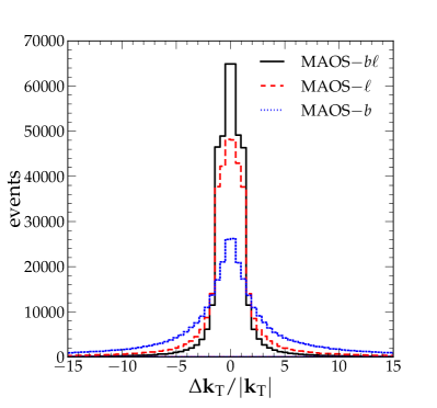
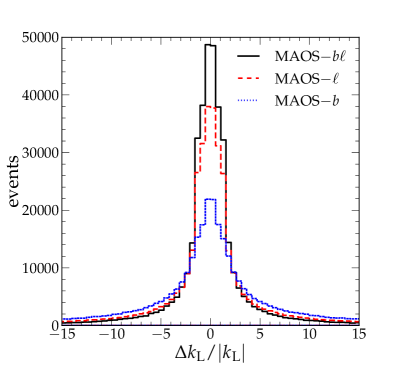
Figure 1: Distributions of $\Delta{\boldsymbol{k}}_{{\rm T}}/|{\boldsymbol{k}}_{{\rm T}}|\equiv({\boldsymbol{k}}_{{\rm T}}^{\rm maos}-{\boldsymbol{k}}_{{\rm T}}^{\rm true})/|{\boldsymbol{k}}_{{\rm T}}^{\rm true}|$ (left panel) and $\Delta k_{\rm L}/|k_{\rm L}|\equiv(k_{\rm L}^{\rm maos}-k_{\rm L}^{\rm true})/|k_{\rm L}^{\rm true}|$ (right panel). $k$ is the neutrino momentum in SM $t\bar{t}$ production (LHC, 14 TeV) followed by a decay to $b\ell\nu$ on both sides. The $x$-axis variable in the left panel stands for either of $\Delta k_{x}$ or $\Delta k_{y}$.

Fig. 1 displays the distributions of $\Delta{\boldsymbol{k}}_{{\rm T}}/|{\boldsymbol{k}}_{{\rm T}}|\equiv({\boldsymbol{k}}_{{\rm T}}^{\rm maos}-{\boldsymbol{k}}_{{\rm T}}^{\rm true})/|{\boldsymbol{k}}_{{\rm T}}^{\rm true}|$ for the different MAOS momenta, showing that $k^{{\rm maos}-b\ell}$ matches best the true neutrino momenta. From the distributions one sees that the vast majority of the MAOS-estimated invisible momenta differ from the true momenta by less than a factor of two in either of the transverse and the longitudinal directions. The $k^{{\rm maos}-\ell}$ performs somewhat worse than $k^{{\rm maos}-b\ell}$, whereas $k^{{\rm maos}-b}$ is not comparable to the others. Henceforth we will thus focus on $k^{{\rm maos}-b\ell}$ and $k^{{\rm maos}-\ell}$.

The difference of efficiency between $k^{{\rm maos}-b\ell}$ and $k^{{\rm maos}-\ell}$ is due to two main reasons. The first one is the trivial $M_{\rm T2}$ zero when all the visible and invisible particles are massless, as is the case for $M_{\rm T2}^{\ell}$ [17]. The trivial-zero solution occurs when the missing transverse momentum $\not{\boldsymbol{p}}_{\rm T}$ lies inside of the smaller of the two cones enclosed between the visible-particle momenta ${\boldsymbol{p}}_{{\rm T}}^{(1)}$ and ${\boldsymbol{p}}_{{\rm T}}^{(2)}$ (see Fig. 2). In such case, the $M_{\rm T2}$ value is attained for a momentum configuration where ${\boldsymbol{k}}_{{\rm T}}^{(i)}$ is proportional to its visible partner momentum ${\boldsymbol{p}}_{{\rm T}}^{(i)}$, thus making the transverse masses in eq. (2) all vanish.

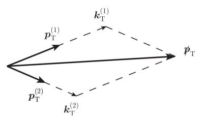
Figure 2: Kinematic configuration for the trivial-zero MAOS solution. See text for details.

The right panels of Fig. 3 show indeed a tower of events in the lowest $M_{\rm T2}^{\ell}$ bin. Application of the MAOS method to real situations requires a suitable $M_{\rm T2}$ cut, excluding events with too small $M_{\rm T2}$ values. In fact, as stated in [12], the MAOS algorithm performs best in events with $M_{\rm T2}$ values closer to the endpoint. Therefore, the trivial-zero solution does not set a fatal limitation to the MAOS method as long as a reasonable $M_{\rm T2}$ lower cut is imposed.

The second reason for the different efficiency between $k^{{\rm maos}-b\ell}$ and $k^{{\rm maos}-\ell}$ is the number of kinematic configurations close to the $M_{\rm T2}^{\rm max}$ value – as we just said, the region where the MAOS algorithm performs best. For instance, in the case of $M_{\rm T2}^{b\ell}$ the visible-particle systems consist of one $b$ quark and one charged lepton. By construction, $M_{\rm T2}^{b\ell}$ depends only on the sum of their momenta, irrespective of the individual momentum magnitudes. This freedom implies that the same $M_{\rm T2}$ value can be attained with different choices of these individual momenta, and the number of these choices is higher for higher $M_{\rm T2}$ values. Hence (many) more kinematical configurations close to the $M_{\rm T2}$ endpoint are possible for $M_{\rm T2}^{b\ell}$ than for $M_{\rm T2}^{\ell}$ and this explains why, close to the endpoint, the $M_{\rm T2}^{b\ell}$ peak is much sharper than the $M_{\rm T2}^{\ell}$ one (cf. left vs. right panels of Fig. 3).

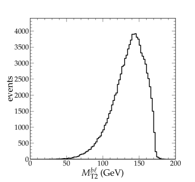
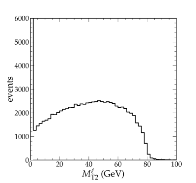
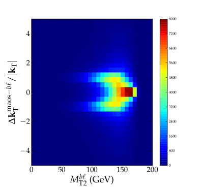
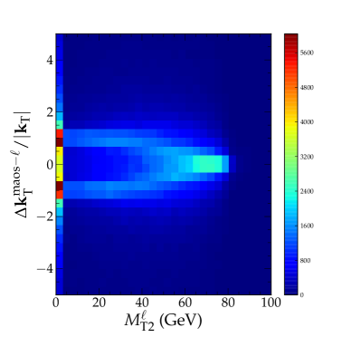
Figure 3: Distributions of (upper frame) $M_{\rm T2}$ and (lower frame) the correlation between $M_{\rm T2}$ and $\Delta{\boldsymbol{k}}_{{\rm T}}$ for (left panels) $k^{{\rm maos}-b\ell}$ and (right panels) $k^{{\rm maos}-\ell}$.

While the first reason (trivial-zero solution) does not occur in cases where the visible and invisible particles are massive, the second reason holds in general: the larger the number of ways to compose individual momenta to obtain the same total visible momentum (the only input needed for $M_{\rm T2}$), the larger the number of events close to the $M_{\rm T2}$ endpoint, where MAOS performs best. From this one can deduce that, in cascade decays involving several steps, the best-performing MAOS momenta are those constructed from the full-system $M_{\rm T2}$.

A final remark on the possible role of initial-state QCD radiation (ISR) is in order. The latter is known [18, 19] to potentially affect the $M_{\rm T2}$ near-endpoint region, that, as we have been arguing, is the region where the MAOS algorithm performs best. We have checked the negligibility of this effect by studying the distributions in Fig. 1 for events with an additional ISR jet, and found no appreciable differences.

Using $k^{{\rm maos}-b\ell}$ we have now a systematic way of estimating the two neutrino momenta, and of thereby reconstructing the $t$ and $\bar{t}$ rest frames. The latter can be used to evaluate top-polarization or $t\bar{t}$ spin-correlation observables, to be studied in the next sections.

3 Top polarization

Top decay products obey angular distributions that are correlated with the parent-top spin. This well known fact is, among quarks, a unique property of the top, and it is due to its large mass. The latter is responsible for the top-quark’s small lifetime, $\sim 1/(G_{F}m_{t}^{3})$, much shorter than the time, $\sim m_{t}/\Lambda_{\rm QCD}^{2}$, needed by QCD interactions to decorrelate the production-time spin configuration [21].

At hadron colliders, top quarks are produced predominantly as $t\bar{t}$ pairs by QCD processes, which a priori cause left and right polarizations to weigh equally in an event set. However, in new-physics scenarios involving chiral couplings, top-quark polarizations may be produced in unequal weights. Accurately measuring the top polarization is therefore considered as an important clue for physics beyond the SM.

One can construct at least two different classes of observables measuring top polarization: energy ratios and the angular distributions of top decay products. We discuss them in turn in the next two subsections.

3.1 Top polarization from ratios of daughter to parent particle energies

One way to test top polarization is via the energy spectra of the top decay products, that may namely be peaked towards softer or harder values depending on the top being left- or right-handed. We will focus here on top production followed by a leptonically-decaying $W$, $t\rightarrow bW(\rightarrow\ell^{+}\nu)$. In Refs. [22, 23] it was pointed out that the chirality of the top quark is correlated with the ratio

$$x_{\ell}=\frac{2E_{\ell^{+}}}{E_{t}}$$ (8)

between the charged-lepton energy and that of its parent top quark. Specifically, charged leptons produced by right-handed top quarks tend to be more energetic than those produced by left-handed top quarks, the difference increasing with the top energy. This conclusion follows from the fact that the $b$-quark is (to very good approximation) always produced left-handed and the $W$ predominantly longitudinal [22, 23].

This feature can easily be checked quantitatively in $pp$ collisions at 14 TeV by generating Monte Carlo events for purely left-handed, purely right-handed, or SM-produced $t\bar{t}$ pairs. The resulting $d\Gamma(t\rightarrow b\ell^{+}\nu)/dx_{\ell}$ distribution at parton level is shown in the left panel of Fig. 4.

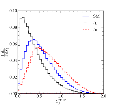
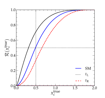
Figure 4: (Left panel) differential distribution of the energy ratio in eq. (8) and (right panel) corresponding cumulative distribution. The three distributions in either plot refer to purely left-handed, or purely right-handed, or QCD-produced tops (see legend). The antitop branches of each event are also included.

The difference between the $t_{L}$ and $t_{R}$ cases can be better appreciated via the integral of the differential distribution up to a given $x_{\ell}=x_{c}$ value:

$$\mathcal{R}(x_{c})\equiv\frac{1}{\Gamma}\int_{0}^{x_{c}}\frac{d\Gamma}{dx_{\ell}}dx_{\ell}~{}.$$ (9)

Qualitatively, this cumulative distribution estimates how early the differential distribution approaches the peak. The cumulative distributions of the histograms in Fig. 4 (left panel) are shown in the right panel of the same figure.

This strategy can be applied to the extent that the top energy can be reconstructed. For example, in $t\bar{t}$ decays where one top decays semi-leptonically and the other hadronically, the momentum of the semi-leptonically decaying top can be reconstructed by using the on-shell relations

$$\left(p^{b}+p^{\ell}+k^{\nu}\right)^{2} =m_{t}^{2}\quad\mbox{or}\quad\left(p^{\ell}+k^{\nu}\right)^{2}=m_{W}^{2},$$

$$(k^{\nu})^{2} =0,\quad{\boldsymbol{k}}_{{\rm T}}^{\nu}=\not{\boldsymbol{p}}_{\rm T}~{}.$$ (10)

Hence $x_{\ell}$ is calculable from eq. (10) up to a discrete degeneracy.

More generally, however, the $t\bar{t}$ pair may be the result of a longer decay chain, involving further undetected particles than just a neutrino – for example supersymmetric $\tilde{t}\,\tilde{t}$ production would lead to $t\bar{t}$ plus two additional neutralinos. In this case $E_{t}$ cannot be reconstructed directly and it is meaningful to search for ‘proxies’ of the variable in eq. (8), that do not involve $E_{t}$. This issue has been recently explored in [25].

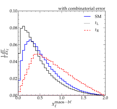
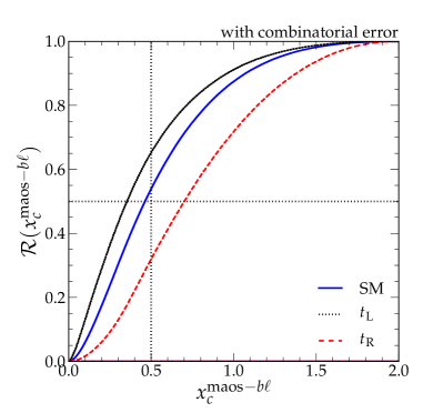
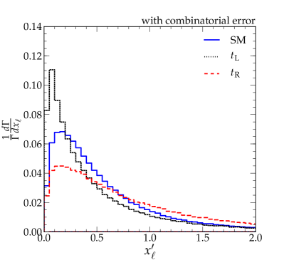
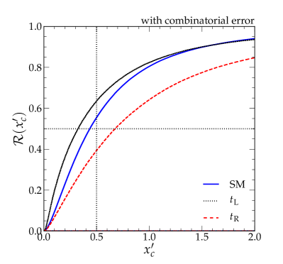
Figure 5: Same as Fig. 4, but with the $x_{\ell}$ variable evaluated with the MAOS method, as in eq. (12) (upper frames), or using the primed variable in eq. (11) [25] (lower frames).

In particular, the authors of [25] consider the case where one of the tops decays as $t\rightarrow b\ell^{+}\nu$ and the other as $\bar{t}\rightarrow\bar{b}q\bar{q}^{\prime}$. The energy of the semileptonically-decaying top, $E_{t}$, is estimated, event by event, via the energy of the other (anti-)top, $E_{\bar{t}}$, that at least in principle is measurable. They thus introduce the modified energy-ratio variable

$$x_{\ell}^{\prime}=\frac{2E_{\ell^{+}}}{E_{\bar{t}}}=\frac{2E_{\ell^{+}}}{E_{\bar{b}}+E_{q}+E_{\bar{q}^{\prime}}}.$$ (11)

The above strategy cannot (or at least is not designed to) be applied in $t\bar{t}$ events where both $W$ decay to leptons, because the two undetected neutrinos in the final state challenge the reconstruction of both $E_{t}$ and $E_{\bar{t}}$. On the other hand, since the $t\bar{t}$ decay topology is suitable for the construction of $M_{\rm T2}$, the parent-particles’ energies can actually be estimated using the MAOS method discussed in the previous section. We accordingly define

$$x_{\ell}^{\rm maos}=\frac{2E_{\ell^{+}}}{E_{t}^{\rm maos}}=\frac{2E_{\ell^{+}}}{E_{b}+E_{\ell^{+}}+E_{\nu}^{\rm maos}},$$ (12)

where $E_{\nu}^{\rm maos}=|{\boldsymbol{k}}^{{\rm maos}-b\ell}|$. Here we choose the MAOS four-momentum estimated from the full-system $M_{\rm T2}$, $k^{{\rm maos}-b\ell}$ (cf. discussion in sec. 2.2). The differential and respectively cumulative (the analogue of eq. (9)) distributions of $x_{\ell}^{\rm maos}$ are shown in the upper frames of Fig. 5. As a comparison, the corresponding distributions for the case of the $x_{\ell}^{\prime}$ variable in eq. (11) are shown in the lower frames of Fig. 5.

It should be noted that application of the $x_{\ell}$ variable to di-leptonic $t\bar{t}$ decays comes, by construction, with an additional uncertainty, namely the two-fold combinatorial ambiguity of correctly assigning the 2 $b$-jets (that are not flavor-tagged, i.e. their charge is not determined in general) + $2\ell$ final state to the two decay chains. We address this ambiguity using the method in [29]. Energy-ratio variables, such as those considered in this section, turn out to be rather robust with respect to the combinatorial error: distributions where this error is taken into account barely differ with respect to those with final states always paired correctly. Hence in this section we only show distributions where this ambiguity is included.

The following comments on Fig. 5 are in order.

1. Since the computation of the MAOS momentum preserves energy-momentum conservation, $E_{\ell}$ is always smaller than $E_{t}^{\rm maos}$, hence the $x_{\ell}^{\rm maos}$ distribution has a definite cutoff at 2, like the $x_{\ell}^{\rm true}$ distribution constructed with the true $E_{t}$, and shown in Fig. 4. Note that, on the other hand, the $x_{\ell}^{\prime}$ differential distribution does not fulfill the same cutoff requirement, as confirmed by the lower plots of Fig. 5.

2. In the cumulative $x_{c}^{\rm maos}$ distribution, the unpolarized case (the SM one) lies neatly between the purely $t_{L}$ and the purely $t_{R}$ cases, in close resemblance to the true distribution. Again, this is largely consequence of the fact that the MAOS distributions fulfill the cutoff constraint mentioned in item 1.

3. From the previous items, one concludes that the distribution constructed with the MAOS method is fairly close to the true distribution already at the differential level. Thus this method allows to test top polarization via the $x_{\ell}$ variable, even in the di-leptonic $t\bar{t}$ decay channel.

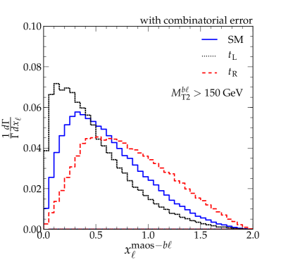
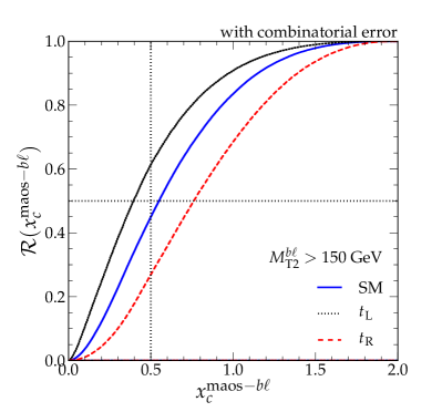
Figure 6: Same as the upper panels of Fig. 5, but including a lower cut on $M_{\rm T2}$.

A further virtue of the MAOS method is that the accuracy of the approximation is under the control of the $M_{\rm T2}$ cut. As mentioned, the MAOS momenta become closer to the true momenta for events with $M_{\rm T2}$ approaching $M_{\rm T2}^{\rm max}$, as shown in the lower left frame of Fig. 3. Therefore, by imposing a suitable $M_{\rm T2}$ cut, the accuracy of the MAOS momentum can be increased at the expense of statistics. Fig. 6 shows the same distributions as in the upper frames of Fig. 5 but with the inclusion of an $M_{\rm T2}^{b\ell}>150$ GeV cut. Note that, because the $M_{\rm T2}$ distribution has a peak structure close to the endpoint (see left panels of Fig. 3), the number of events not passing this cut is (only) half of the total dataset. By comparing Fig. 6 with Figs. 5 and 4, one can see that the cumulative MAOS distribution is close to the true distribution, and that the distribution with the $M_{\rm T2}$ cut gets even closer to it. In fact, the inclusion of the $M_{\rm T2}$ cut is above all intended to check explicitly that it does not introduce distortions in the overall distributions. This would occur if the cut selected kinematic configurations more populated e.g. by $t_{R}$ than by $t_{L}$, so as to introduce cut-induced asymmetries.

3.2 Top polarization from angular variables

The MAOS method allows full reconstruction of the parent-particle’s momentum. This permits to test the most direct of top-polarization observables, the angular distribution of top decay products. Among the latter, charged leptons have the double advantage of a ‘maximal’ spin-analyzing power [30] and of being especially clean objects for experiments. At tree level, the charged-lepton distribution in top-quark decays can be written as (see e.g. [31])

$$\frac{1}{\Gamma}\frac{d\Gamma}{d\cos\theta}=\frac{1+\alpha\cos\theta}{2},$$ (13)

where $\theta$ denotes the angle between the decaying-particle spin-quantization axis and the direction of the charged lepton, viewed in the decaying-particle’s rest frame. The coefficient $\alpha$ denotes the mentioned charged-lepton spin-analyzing power, equalling $+1~{}(-1)$ for spin-up (spin-down) tops or spin-down (spin-up) antitops. Angular distributions from decay products other than charged leptons obey relations entirely analogous to eq. (13), but for a different spin-analyzing power $|\alpha|\leq 1$.

By its definition, to calculate the angle $\theta$ one should reconstruct the top rest frame. The $\cos\theta_{\ell}$ distribution in $t\bar{t}$ production followed by a leptonic decay of both $W$ is shown in Fig. 7, where we have used the true top rest frames. The figure shows graphically the very distinct $\cos\theta_{\ell}$ behavior between the $t_{L}$ and the $t_{R}$ cases dictated by eq. (13).

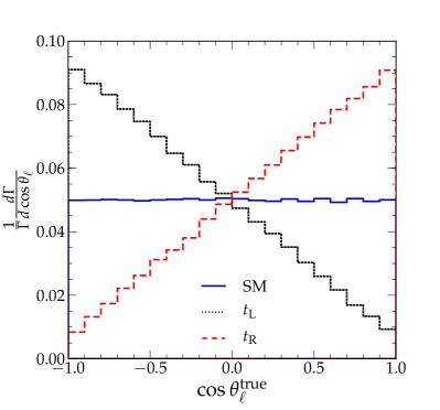
Figure 7: The distributions of $\cos\theta_{\ell}$ using the true top-quark momentum.

Fig. 7 is purely theoretical, because the two neutrinos in the final state challenge the reconstruction of the rest frames of the two tops. Experimentally, event reconstruction in this case is performed via maximum-likelihood criteria, such as the neutrino-weighting method [38], used in [39], or matrix-element weighting techniques [40], as in [41] (cf. also sec. 3.3).

We attempt this reconstruction with the MAOS method, and denote the correspondingly calculated angle as $\theta_{\ell}^{{\rm maos}}$. Specifically, we again calculate the neutrino momenta from the full-system $M_{\rm T2}$. Denoting them as $k^{(i){\rm maos}-b\ell}$, the parent-particle boost is reconstructed event by event as $p_{t(\bar{t})}^{{\rm maos}-b\ell}=p_{b}+p_{\ell}+k^{(i){\rm maos}-b\ell}$, with $i=1,2$ labelling the $t$ or $\bar{t}$ decay chain. The resulting distributions for purely left-, purely right-handed, and SM $t\bar{t}$ production are shown in the left panel of Fig. 8.

Two observations are in order. First, the just mentioned reconstruction of the $p_{t(\bar{t})}$ momenta suffers from the combinatorial ambiguity of correctly pairing the two $b$-jets with the two charged leptons. The left panel of Fig. 8 does not include this combinatorial ambiguity – the $b\ell$ pairings are namely taken to be the correct ones. This plot is meant to show the modifications with respect to the true distributions, coming from the MAOS reconstruction alone. The combinatorial error is included in the right panel of Fig. 8. This error can be straightforwardly addressed by implementing the four ($M_{\rm T2}$-based) test variables proposed in [29]. We find that the method correctly assigns the two $b\ell$ pairs in 83% of the events, before any cut. Henceforth, we will refer to the method’s percentage of events with correctly assigned pairs as efficiency.

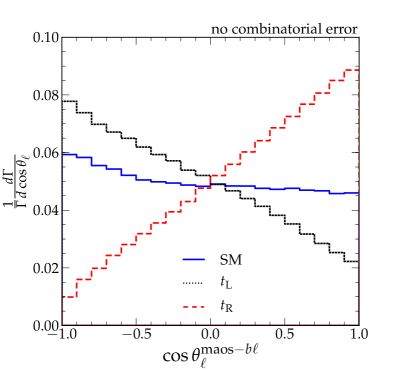
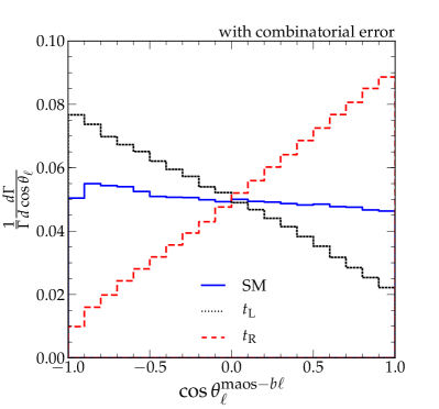
Figure 8: The distributions of $\cos\theta_{\ell}$ using the MAOS-reconstructed top-quark momentum without (left panel) and with (right panel) inclusion of the $b\ell$-assignment combinatorial ambiguity (see text).

A second observation concerns the (only) non-negligible distortion of the MAOS-reconstructed distributions with respect to the truth-level ones. This distortion, as apparent from Fig. 8, occurs for leptons produced in the backward direction ($\cos\theta_{\ell}\approx-1$), that is well populated in the $t_{L}$ and SM cases. We have investigated in detail the origin of this distortion. A first general explication is the fact that this region is inherently unfavorable for the application of the MAOS algorithm. In fact, leptons produced backwards with respect to the parent tops have an energy spectrum peaked towards softer values (see e.g. Fig. 4, left), whereas the MAOS-algorithm reliability increases with larger visible momenta, as detailed in sec. 2.2. Another, more technical, reason for the distortion is the fact that kinematic configurations with one of the visible daughter particles produced backwards with respect to the parent tend more often to have an ‘unbalanced’ $M_{\rm T2}$ value [4, 43, 44]. (Namely the ${\boldsymbol{k}}_{{\rm T}}^{(1)}$, ${\boldsymbol{k}}_{{\rm T}}^{(2)}$ configuration yielding $M_{\rm T2}$ is such that $M_{\rm T2}={\rm max}\{M_{{\rm T}}^{(1)},M_{{\rm T}}^{(2)}\}$, with $M_{{\rm T}}^{(1)}\neq M_{{\rm T}}^{(2)}$. On the other hand, in a balanced solution one has by definition $M_{\rm T2}=M_{{\rm T}}^{(1)}=M_{{\rm T}}^{(2)}$.) Invisible momenta reconstructed from unbalanced $M_{\rm T2}$ solutions are more likely to deviate from the true momenta than if they come from balanced $M_{\rm T2}$ solutions. As a check, we have repeated Fig. 8 (left), but excluding events with unbalanced $M_{\rm T2}$ solutions, and indeed the distortion gets mildened.

Both of these effects – the combinatorial ambiguity and the $\cos\theta_{\ell}^{+}\approx-1$ distortion – can be systematically improved by selecting events with $M_{\rm T2}$ closer to its endpoint, where incidentally the MAOS algorithm itself is known [12] to be more reliable – see lower-left panel of Fig. 3. Furthermore, a lower cut on $M_{\rm T2}$ represents a standard cut in detector-level analyses. In Fig. 9 we show histograms which differ from those in Fig. 8 for the application of an $M_{\rm T2}>150$ GeV cut, that halves the number of events. The figure demonstrates how the cut indeed effects positively both the MAOS method alone (left panel) as well as the MAOS method with combinatorial error included (right panel). It should also be noted that in the right panel of Fig. 9 the above-discussed distortion has largely disappeared.

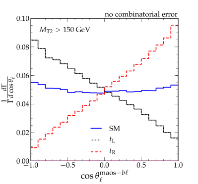
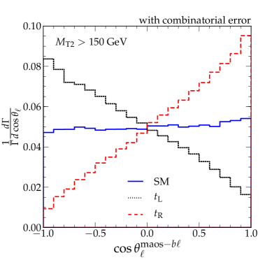
Figure 9: Same as Fig. 8, but for the inclusion of an $M_{\rm T2}$ cut.

All in all, from the sequence of plots in Figs. 8 - 9 one can draw three non-trivial conclusions: (i) the MAOS reconstruction of the invisible momenta is accurate enough for top-polarization distributions not to be appreciably distorted with respect to the true ones; (ii) the combinatorial error (intrinsic to the method, at least for the full-system $M_{\rm T2}$ case) has in fact a marginal impact on the MAOS reconstruction; (iii) this error can be systematically controlled by the same sort of cuts that also help the MAOS method itself.

As a side comment to item iii, we note that in fact the most effective cut to improve the efficiency of the combinatorial method is a lower cut on the full-system transverse mass $M_{{\rm T}}^{t\bar{t}}$ (see ref. [29] for quantitative details). The interesting aspect is that this variable is correlated with the overall boost of the $t\bar{t}$ system – the harder the $M_{{\rm T}}^{t\bar{t}}$ cut, the more boosted the selected $t\bar{t}$ sample. Therefore, we expect our method to perform very well also in the boosted regime.

A more realistic comparison between the truth-level and the MAOS-reconstructed distributions would involve the inclusion of a set of cuts such that the selected event sample resemble as much as possible the one selected by the experimental trigger, as well as the simulation of hadronization and energy-momentum smearing effects. We refrain from a refined analysis of this kind in a theory study. Similarly as in [45], we limit ourselves to the introduction of two ‘minimal’ centrality cuts, that approximately identify the kinematic fiducial region of the $t\bar{t}$ sample. From the recent Atlas analysis [46], we conservatively take these cuts to be $p_{{\rm T}}>20$ GeV and $|\eta|<2.5$, applied to all final states. We show in Fig. 10 how the true distribution (cf. Fig. 7) and the MAOS-reconstructed one (cf. right panel of Fig. 9) are modified by the introduction of these cuts. As expected, the main effect is to underpopulate the bins with $\cos\theta_{\ell}$ close to $-1$, where the charged lepton tends to be softer, as already discussed. Noteworthy is that this distortion effects the true and the MAOS-reconstructed distribution in a very similar way.

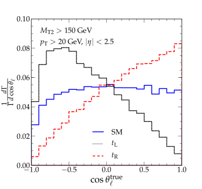
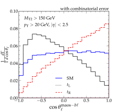
Figure 10: Comparison between the true (cf. Fig. 7) and the MAOS-reconstructed (cf. right panel of Fig. 9) distributions, but for the inclusion of a $p_{{\rm T}}$ and an $|\eta|$ cut. In the true distribution (left panel) we also include an $M_{\rm T2}$ cut for consistency with the analysis of the MAOS-reconstruced distribution (right panel).

A more quantitative idea of the difference between all the discussed cases may be obtained by calculating the asymmetry observable

$$\mathcal{A_{\ell}}=\frac{\sigma(\cos\theta_{\ell}>0)-\sigma(\cos\theta_{\ell}<0)}{\sigma(\cos\theta_{\ell}>0)+\sigma(\cos\theta_{\ell}<0)}~{}.$$ (14)

Table 1 collects the values of this asymmetry, calculated for the true distribution vs. the MAOS-reconstructed one for purely left-handed, purely right-handed, or SM-produced $t\bar{t}$ pairs (table columns) and without or with inclusion of the most significant cuts and effects discussed (table rows). To limit clutter, we have labelled the considered cases by the corresponding figure. These cases include, in order of descending row, the following distributions: (i) the true one; (ii) the MAOS-reconstructed one, without combinatorial error or cuts; (iii) the MAOS one, including combinatorial error and the $M_{\rm T2}$ cut; (iv) the true one, with $p_{{\rm T}}$ and $\eta$ cuts included; (v) the MAOS one as in item iii, with $p_{{\rm T}}$ and $\eta$ cuts included. As previously discussed in detail, the most relevant comparisons are between cases (i) and (iii) and between cases (iv) and (v).

	$t_{L}$	$t_{R}$	SM
$\mathcal{A}_{\ell}^{{\rm true}\phantom{s}}$ (Fig. 7)	$-0.43$	$0.43$	$-0.001$
$\mathcal{A}_{\ell}^{\rm maos}$ (Fig. 8, left)	$-0.27$	$0.41$	$-0.05$
$\mathcal{A}_{\ell}^{\rm maos}$ (Fig. 9, right)	$-0.33$	$0.42$	$0.03$
$\mathcal{A}_{\ell}^{{\rm true}\phantom{s}}$ (Fig. 10, left)	$-0.37$	$0.38$	$0.05$
$\mathcal{A}_{\ell}^{\rm maos}$ (Fig. 10, right)	$-0.28$	$0.40$	$0.07$

Table 1: Numerical comparison of the MAOS-reconstructed vs. truth-level $\mathcal{A}_{\ell}$ as defined in eq. (14). The considered cases (table rows) are labelled by the corresponding figure. The $t\bar{t}$ pairs are assumed to be purely left-handed, purely right-handed, or produced via SM QCD (table columns).

3.3 Remarks on the method’s comparison with existing ones

Having introduced all the main method’s features in a concrete application, it is worthwhile to comment at this point on how ours compares to existing methods aimed at the reconstruction of the $t$ and $\bar{t}$ boosts in di-leptonic $t\bar{t}$ decays. As already mentioned in sec. 3.2, these ‘likelihood-based’ methods include the neutrino weighting ($\nu$W) method [38] as well as the matrix-element weighting (MEW) one [40].

Each of these methods involves as a crucial step the construction of weighting functions (based on Monte Carlo procedures) to estimate the likelihood of each of the possible solutions for the neutrino momenta compatible with the system of kinematic equations.

We advance the following remarks on the various methods.

• Both methods, ours and the likelihood methods, are kinematics-based: in the likelihood methods one solves a system of equations corresponding to all kinematic constraints; in ours one uses an $M_{\rm T2}$ property that somewhat summarizes these very kinematic constraints.

• One difference is in the treatment of the resulting kinematic solutions. We expect that the robustness of the $\nu$W and MEW methods will depend on the reliability of the Monte Carlo used to determine the weighting function. On the other hand, our method relies solely on kinematics, namely on the decay topology being suitable for the construction of $M_{\rm T2}$.

• Still concerning the kinematic information used, we further remark that likelihood methods use both of the $m_{W}$ and $m_{t}$ constraints, that actually differ event by event due to the finite $W$ and $t$ widths. On the other hand, the MAOS method is using only one of these mass constraints, $m_{t}$ in the case of $M_{\rm T2}^{b\ell}$. The explicit use of less kinematic information may be beneficial to reduce the associated systematic uncertainty.

• The accuracy of the MAOS method can be controlled by an $M_{\rm T2}$ cut, as long as the statistics permits it, as is expectedly the case at LHC14. We are not aware of a systematic and intuitive way to control accuracy in likelihood methods.

In general, it is to be expected that the information from one method will improve the efficiency of the other ones (and vice versa). Therefore, barring strong correlations across the methods, the best overall reconstruction efficiency will be obtained by integrating (and optimizing accordingly) the MAOS method with the other ones.

4 Spin correlations in $t\bar{t}$ production

Top polarization may be unobservable if its production mechanism involves $t_{L}$ and $t_{R}$ in similar fractions. This is the case in the SM, where tops are produced dominantly as $t\bar{t}$ pairs by QCD interactions, which weigh equally left-handed and right-handed components. The SM distribution in Fig. 7 is in fact unobservably flat (cf. also top-polarization asymmetries in the last column of Table 1). In these circumstances, the different spin components in $t\bar{t}$ production can still be tested by looking at spin correlations between $t$ and $\bar{t}$. The latter impart correlations between the angular distribution of decay product $i$ from the top and the angular distribution of decay product $\bar{i}$ from the anti-top. The doubly-differential (with respect to these two decay products) distribution can be written as [47]

$$\frac{1}{\sigma}\frac{d^{2}\sigma}{d\cos\theta_{i}\,d\cos\theta_{\bar{i}}}~{}=~{}\frac{1\,+\,C_{t\bar{t}}\,\alpha_{i}\alpha_{\bar{i}}\,\cos\theta_{i}\cos\theta_{\bar{i}}}{4}~{},$$ (15)

where $\theta_{i(\bar{i})}$ is the angle between the chosen spin-quantization axis and the direction of decay product $i(\bar{i})$, viewed in the respective mother-particle’s rest frame, and $\alpha_{i(\bar{i})}$ has already been introduced below eq. (13). Furthermore

$$C_{t\bar{t}}~{}=~{}\frac{\sigma_{t_{\uparrow}\bar{t}_{\uparrow}}+\sigma_{t_{\downarrow}\bar{t}_{\downarrow}}-\sigma_{t_{\uparrow}\bar{t}_{\downarrow}}-\sigma_{t_{\downarrow}\bar{t}_{\uparrow}}}{\sigma_{t_{\uparrow}\bar{t}_{\uparrow}}+\sigma_{t_{\downarrow}\bar{t}_{\downarrow}}+\sigma_{t_{\uparrow}\bar{t}_{\downarrow}}+\sigma_{t_{\downarrow}\bar{t}_{\uparrow}}}~{},$$ (16)

where the symbols on the r.h.s. denote the cross sections for production of $t\bar{t}$ pairs in either of the four possible spin configurations, with $\uparrow$ ($\downarrow$) denoting a particle with spin up (down) with respect to the chosen spin-quantization axis.

Spin correlations within the SM, as well as the question how they can best be measured at hadron colliders, have been extensively studied  [31, 48, 49, 50, 45, 51, 52, 47]. Given the $C_{t\bar{t}}$ dependence in eq. (15), it is clear that spin correlations are larger when $C_{t\bar{t}}$ increases in magnitude, namely when the difference between like- and unlike-spin $t\bar{t}$ pairs is maximal. One crucial insight by Mahlon, Parke and Shadmi [31, 50, 45] is the realization that this difference can be maximized by an appropriate choice of the spin-quantization axis. Once the appropriate basis choice is made, the $t\bar{t}$ cross section turns out to be dominated by one single spin configuration. This ‘optimal’ basis choice is different between the Tevatron and the LHC.

At Tevatron, $t\bar{t}$ pairs are produced dominantly through $q\bar{q}$ annihilation. For this process, it has been shown [50, 45] that one can choose a spin basis in which the like-spin $t\bar{t}$ components ($t_{\uparrow}\bar{t}_{\uparrow}$ and $t_{\downarrow}\bar{t}_{\downarrow}$) in the cross section vanish identically, and this basis is referred to as the ‘off-diagonal’ basis [50]. A very useful parameterization of the corresponding spin eigenvector is provided by Uwer in [52]. In the $t\bar{t}$ rest frame, the angle between the incoming beam (usually identified with $+\hat{z}$) and the top spin axis reads

$$\tan\psi~{}=~{}\frac{\tan\theta\left(1-\gamma^{-1}\right)}{1+\gamma^{-1}\tan^{2}\theta}~{},$$ (17)

with $\theta$ the top-quark scattering angle with respect to $\hat{z}$ and $\gamma=1/\sqrt{1-\beta^{2}}$, $\beta$ being the top-quark speed. Note that, close to threshold ($\gamma\rightarrow 1$), the spin axis becomes aligned to the beam axis, so that in this limit one recovers the ‘beam-line’ basis [31], whereas at very high energies ($\gamma\gg 1$), the spin axis becomes aligned to the top-momentum direction, it namely coincides with the ‘helicity’ basis [31]. Concretely, for $t\bar{t}$ pairs dominantly produced close to threshold, as was the case at Tevatron, the off-diagonal basis lies close to the beamline basis for all scattering angles [50]. For Tevatron data, this suggests to use the off-diagonal basis as the optimal choice for spin-correlation studies, and the beamline basis as a sub-optimal choice [50, 45].

At the LHC, $t\bar{t}$ pairs are produced dominantly through $gg$ fusion. For $gg\rightarrow t\bar{t}$, there is no basis where the $t\bar{t}$ pairs are in purely like- or unlike-spin configurations, because this basis is different depending on whether $gg$ are in like- or unlike-helicity configurations, and in general both helicity components are present in the $gg\rightarrow t\bar{t}$ cross section [47, 52]. An ‘optimized’ spin-basis choice can still be made according to whether the $gg$ pair is dominantly in a like- or unlike-helicity configuration [47], which in turn depends on the center-of-mass energy of the $pp$ collisions, or equivalently on $M_{t\bar{t}}$. Specifically, at low $M_{t\bar{t}}$, $gg$ pairs are dominantly produced with like helicities. In this case, the amplitudes squared yielding $t\bar{t}$ pairs in unlike-spin configurations can be made to vanish (for all $\beta$) in the helicity basis [47]. Conversely, at (very) high $M_{t\bar{t}}$, $gg\rightarrow t\bar{t}$ occurs dominantly via unlike-helicity gluons. In this case, the amplitudes squared to $t\bar{t}$ in like-spin configurations vanish in the off-diagonal basis [47], similarly as in the $q\bar{q}\rightarrow t\bar{t}$ case seen in the previous paragraph. However, as noted in [47], the fraction of $t\bar{t}$ pairs produced in this ultrarelativistic limit at the LHC (with 14 TeV collision energy) is very small. One concludes that, at the LHC with 14 TeV, $t\bar{t}$ spin correlations are well described in the helicity basis [31, 47]. We will then use this basis for our reference study of $t\bar{t}$ spin correlations reconstructed via the MAOS algorithm. We will afterwards address the case where an ‘optimized’ basis is used.

4.1 MAOS-reconstructed spin correlations in the helicity basis

From eq. (15) it is clear that, along with an accurate choice of the spin-quantization axis, it is also essential to choose correctly the final states $i$ and $\bar{i}$ – different states have different spin-analyzing power, and pose different detection challenges [53, 48]. In this paper, since we are focusing on kinematic methods based on $M_{\rm T2}$, we confine ourselves to $t\bar{t}\rightarrow b\ell^{+}\bar{\nu}\,\bar{b}\ell^{-}\nu$ and take $i=\ell^{+}$ and $\bar{i}=\ell^{-}$. As already remarked, di-leptonic $t\bar{t}$ decays have the advantage that the charged-leptons’ spin-analyzing power is maximal, $|\alpha_{\ell^{+}}|=|\alpha_{\ell^{-}}|=1$, and that $\ell^{\pm}$ are clean objects experimentally, and the drawback of two final-state neutrinos, that hinder the reconstruction of the $t$ and $\bar{t}$ rest frames, required by the $\theta_{\ell^{\pm}}$ definition. Experimentally, the two main techniques used [38, 40] have already been mentioned in the context of top polarization. They have been applied in $t\bar{t}$ spin correlation studies in [54].

In sec. 3.2 on top polarization we have estimated these angular variables using the MAOS-reconstructed invisible momenta $k^{(i){\rm maos}-b\ell}$. We namely calculated the $t$ or $\bar{t}$ rest frames as $p_{t(\bar{t})}^{{\rm maos}-b\ell}=p_{b}+p_{\ell}+k^{(i){\rm maos}-b\ell}$, using the values for the invisible momenta that yield $M_{\rm T2}$ for the event, and reconstructed the angles $\theta_{\ell^{\pm}}$ accordingly. Here we apply this technique to reconstruct the $t\bar{t}$ spin-correlation in eq. (15).

As in the top-polarization study, we provide truth-level distributions as a reference. A convenient quantity to measure the ‘size’ of $t\bar{t}$ spin correlations from the distribution in eq. (15) is the asymmetry [48]

$$A_{\ell\ell}~{}\equiv~{}\frac{N(\cos\theta_{\ell^{+}}\cos\theta_{\ell^{-}}>0)-N(\cos\theta_{\ell^{+}}\cos\theta_{\ell^{-}}<0)}{N(\cos\theta_{\ell^{+}}\cos\theta_{\ell^{-}}>0)+N(\cos\theta_{\ell^{+}}\cos\theta_{\ell^{-}}<0)}~{}=\frac{1}{4}C_{t\bar{t}}\,\alpha_{\ell^{+}}\alpha_{\ell^{-}}~{},$$ (18)

where $N$ denotes the number of events satisfying the condition in parentheses, and we have specialized the notation to di-leptonic $t\bar{t}$. This asymmetry may be visualized from the dependence of the differential distribution in eq. (15) on the product $\cos\theta_{\ell^{+}}\,\cos\theta_{\ell^{-}}$. In Fig. 11 we show such dependence in the case of the true distribution of $t\bar{t}$ produced in $pp$ collisions at 14 TeV (as well as via the subprocesses $gg$ and $q\bar{q}$). The superscript ‘true’ in the $x$-axis emphasizes that in this plot the $t$ and $\bar{t}$ rest frames are calculated using the true neutrino momenta, and also assigning the correct $b\ell$ pairs to the two decay chains, i.e. without including combinatorial ambiguities.

We now turn to the MAOS-reconstructed version of the histograms in Fig. 11. The equivalent histograms, namely including no other uncertainty than the one due to MAOS-estimated $t$ and $\bar{t}$ boosts rather than the true boosts, are shown in the left panel of Fig. 12. In the right panel, we also include the combinatorial ambiguity of assigning the two $b\ell$ pairs to the $t$ and $\bar{t}$ decay chains. This ambiguity is addressed via the same method [29] as the one used in the top-polarization study, sec. 3.2. Fig. 12 provides an already non-trivial test: the clear-cut asymmetry visible in Fig. 11 is still present in the histogram with MAOS-reconstructed momenta and combinatorial ambiguity included.

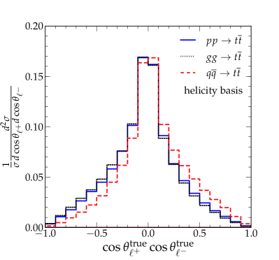
Figure 11: The differential distribution in eq. (15) as a function of $\cos\theta_{\ell^{+}}\cos\theta_{\ell^{-}}$ for $t\bar{t}$ produced from $pp$ collisions at 14 TeV and by its subprocesses $gg$ and $q\bar{q}$ (see legend). Spin axes are in the helicity basis.

Inspection of Fig. 12 reveals that the asymmetry is more pronounced after inclusion of the combinatorial error (right panel) than before it (left panel). This is due to the fact that the efficiency of the combinatorial method is higher in the $\cos\theta_{\ell^{+}}\cos\theta_{\ell^{-}}<0$ region than in the $\cos\theta_{\ell^{+}}\cos\theta_{\ell^{-}}>0$ one: it equals 87% vs. 79% before cuts. As a consequence, some of the wrongly-paired solutions belonging to $\cos\theta_{\ell^{+}}\cos\theta_{\ell^{-}}>0$ will migrate to the other region, whereas the converse will happen less likely. So, while the MAOS method ignoring combinatorial ambiguities slightly dilutes the asymmetry in Fig. 11, the inclusion of combinatorial ambiguities largely compensates this dilution, yielding an asymmetry closer to the truth-level one.

The spurious asymmetry component induced by the treatment of combinatorial ambiguities can be made to disappear by a suitable $M_{\rm T2}$ cut. In fact, the latter reduces substantially the difference between the negative and the positive $x$-axis efficiencies – with the cut $M_{\rm T2}>150$ GeV, the two efficiencies equal 92% vs. 91%. In Fig. 13 we show the same MAOS distributions as Fig. 12, but for the inclusion of the requirement $M_{\rm T2}>150$ GeV. As already discussed, the introduction of an $M_{\rm T2}$ cut is beneficial to the MAOS-reconstruction reliability, and in fact the left panel of Fig. 13 displays a larger asymmetry than the corresponding panel of Fig. 12. Turning to the right panel of Fig. 13, where the combinatorial uncertainty is taken into account, we note that the asymmetry is increased with respect to the case of no cut.

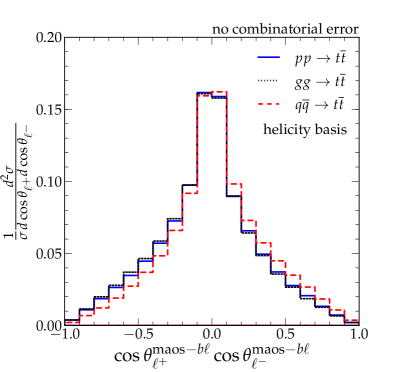
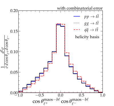
Figure 12: Same distributions as in Fig. 11, but with MAOS-reconstructed $t$ and $\bar{t}$ boosts (see text). The left panel does not include the $b\ell$ combinatorial ambiguity, which is instead taken into account in the right panel.

We observe in this respect that, per se, an $M_{\rm T2}$ cut has the effect of increasing the asymmetry – already at the level of the true distribution. For example, the asymmetry $A_{\ell\ell}$ (18) in the $pp$ case equals $-0.087$ for the truth-level distribution of Fig. 11 (cf. also Table 2 to follow) and reaches $-0.114$ for the same histogram in presence of an $M_{\rm T2}>150$ GeV cut.

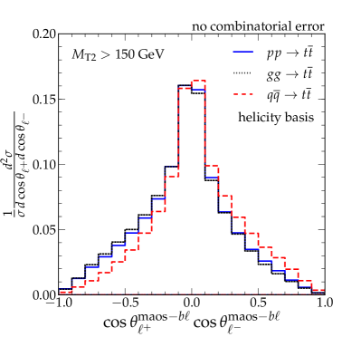
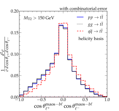
Figure 13: Same distribution as Fig. 12, but for the introduction of an $M_{\rm T2}>150$ GeV cut.

As a final comparison of the MAOS-reconstructed distribution with respect to the truth-level one, we include in both cases the two minimal centrality cuts $p_{{\rm T}}>$ 20 GeV and $|\eta|<2.5$, as already discussed in the top-polarization study (cf. end of sec. 3.2). The resulting distributions are shown in Fig. 14. Worth remarking is the fact that the $p_{{\rm T}}$ and $|\eta|$ cuts do not introduce major distortions in these distributions. As seen in the top-polarization discussion, this sort of cuts is expected to underpopulate the kinematic region where one of the charged leptons is produced backwards with respect to the parent, $\cos\theta_{\ell}\approx-1$. Since the angle of the other lepton is generic, the effect is diluted in the whole $\cos\theta_{\ell^{+}}\cos\theta_{\ell^{-}}\in[-1,+1]$ range, and does not visibly affect Fig. 14.

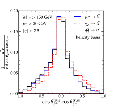
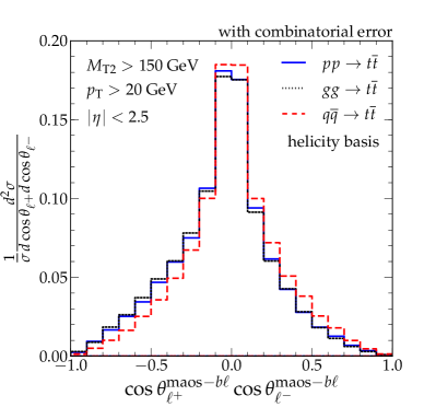
Figure 14: Comparison between the true (cf. Fig. 11) and the MAOS-reconstructed (cf. right panel of Fig. 13) spin-correlation distributions, but for the inclusion of a $p_{{\rm T}}$ and an $|\eta|$ cut. In the true distribution (left panel) we also include an $M_{\rm T2}$ cut for consistency with the analysis of the MAOS-reconstruced distribution (right panel).

We conclude this section by calculating the asymmetry parameter $A_{\ell\ell}$ defined in eq. (18) in the most representative among the cases discussed. These values are collected in Table 2. The considered cases include (in order of descending row): (i) the true asymmetry, without inclusion of any errors or cuts; (ii) the corresponding MAOS-reconstructed asymmetry, again without errors or cuts; (iii) the MAOS asymmetry, with inclusion of the combinatorial ambiguity and of an $M_{\rm T2}$ cut; (iv) the true asymmetry, with inclusion of centrality cuts on $p_{{\rm T}}$ and $|\eta|$; (v) the MAOS asymmetry as in item iii, and including the centrality cuts. The most significant comparisons are between cases (i) and (iii), and between cases (iv) and (v).

helicity basis	$pp$	$gg$	$q\bar{q}$
$A_{\ell\ell}^{{\rm true}\phantom{s}}$ (Fig. 11)	$-0.087$	$-0.12$	$0.11$
$A_{\ell\ell}^{\rm maos}$ (Fig. 12, left)	$-0.055$	$-0.075$	$0.060$
$A_{\ell\ell}^{\rm maos}$ (Fig. 13, right)	$-0.15$	$-0.16$	$-0.003$
$A_{\ell\ell}^{{\rm true}\phantom{s}}$ (Fig. 14, left)	$-0.11$	$-0.13$	$0.080$
$A_{\ell\ell}^{\rm maos}$ (Fig. 14, right)	$-0.11$	$-0.13$	$0.009$

Table 2: Numerical comparison of the MAOS-reconstructed vs. the truth-level spin-correlation asymmetry $A_{\ell\ell}$ as defined in eq. (18) and calculated in the helicity basis. The considered cases (table rows) are labelled by the corresponding figure. The initial states (table columns) are $pp$ at 14 TeV, or its $gg$ or $q\bar{q}$ subprocesses.

4.2 MAOS-reconstructed spin correlations in a boost-dependent basis

As discussed at the beginning of sec. 4, unlike the case of $q\bar{q}\rightarrow t\bar{t}$ one cannot define an optimal basis to calculate $t\bar{t}$ spin correlations in the case of $gg\rightarrow t\bar{t}$ [47, 52], because the optimal basis is different for like- or unlike-helicity $gg$, and both helicity components are present for $gg$ colliding via $pp$ pairs. In practice though, the relative weights of the different helicity components change with the collision energy, and one may define a $\sqrt{s}$-dependent spin-quantization basis according to the helicity component that is dominant at that $\sqrt{s}$. A numerical approach to this possibility was presented in [52], and an analytic solution in [47]. This paper identifies the relation $\beta\gamma\sin\theta=1$ as the kinematic condition separating the region where like-helicity $gg$ dominate ($\beta\gamma\sin\theta\ll 1$) from the one where unlike-helicity $gg$ do ($\beta\gamma\sin\theta\gg 1$). Then, in the first (second) region one can define a $\beta$- and $\theta$-dependent spin-quantization axis that maximizes the $t_{\uparrow}\bar{t}_{\uparrow}+t_{\downarrow}\bar{t}_{\downarrow}$ ($t_{\uparrow}\bar{t}_{\downarrow}+t_{\downarrow}\bar{t}_{\uparrow}$) fractions. We henceforth refer to this axis as $\psi_{\rm like}$ ($\psi_{\rm unlike}$), in the notation of eq. (17). As a practical approximation to this basis, Ref. [47] suggests to use the helicity (off-diagonal) basis in the $\beta\gamma\sin\theta<1$ ($>1$) region. This suggestion can be understood by noting that the region $\beta\gamma\sin\theta\ll 1$ ($\gg 1$) can be identified with the near-threshold (ultra-relativistic) regime, and by recalling that, at the LHC, the helicity basis performs well near threshold, while the off-diagonal basis does so in the ultra-relativistic regime (cf. beginning of sec. 4).

hybrid basis	$pp$	$gg$	$q\bar{q}$
$A_{\ell\ell}^{{\rm true}\phantom{s}}$ (Fig. 11)	$-0.072$	$-0.11$	$0.13$
$A_{\ell\ell}^{\rm maos}$ (Fig. 12, left)	$-0.047$	$-0.067$	$0.073$
$A_{\ell\ell}^{\rm maos}$ (Fig. 13, right)	$-0.13$	$-0.15$	$0.030$
$A_{\ell\ell}^{{\rm true}\phantom{s}}$ (Fig. 14, left)	$-0.078$	$-0.11$	$0.13$
$A_{\ell\ell}^{\rm maos}$ (Fig. 14, right)	$-0.095$	$-0.11$	$0.052$

Table 3: Same as Table 2, but for the use of the hybrid basis (see text) in place of the helicity basis.

We have repeated the helicity-basis study of sec. 4.1 in the basis suggestion of Ref. [47]. We will henceforth refer to this choice as the ‘hybrid’ basis. Our results for $A_{\ell\ell}$ in this basis are collected in Table 3. By comparing this table with Table 2 one immediately notes that the hybrid basis indeed improves the $q\bar{q}$ component of our spin-correlation asymmetries, but it slightly worsens the $gg$ component, which is however the dominant one in $pp$ collisions. As a consequence, we find the helicity basis [31] to performs globally better than the hybrid basis.

A few comments on these findings are in order. First, we note explicitly that, by construction, the hybrid basis coincides with the helicity basis for $\beta\gamma\sin\theta<1$, including the near-threshold region. By looking at the $pp\rightarrow t\bar{t}$ production cross section at 14 TeV, one easily realizes that the overwhelming majority of $t\bar{t}$ pairs is produced in this region. From this argument alone, it is clear that any difference between the helicity and the hybrid basis will affect only the tail of the 14 TeV $t\bar{t}$ distribution. A second observation concerns the $\beta\gamma\sin\theta>1$ region, where the hybrid basis becomes the off-diagonal one. In fact, it is worth remarking that, for $\beta\gamma\sin\theta>1$ the off-diagonal basis tends analytically to the optimal basis, indicated above by $\psi_{\rm unlike}$, only for $\cos\theta\rightarrow 0$ [47]. Away from this limit, deviations between the two bases occur, and it is not obvious how these deviations affect a given observable. In this respect, it should be noted that, while for $\beta\gamma\sin\theta<1$ like-helicity $gg$ pairs clearly dominate the cross section ($gg_{\rm like}:gg_{\rm unlike}=55\%:20\%$), for $\beta\gamma\sin\theta>1$ unlike-helicity $gg$ pairs dominate the cross section only slightly ($gg_{\rm unlike}:gg_{\rm like}=15\%:10\%$) [47].

Our finding that the helicity basis performs somewhat better than the hybrid one for the spin-correlation asymmetry (18) is specific to SM $pp\rightarrow t\bar{t}$ production at 14 TeV. At higher collision energies and in presence of new physics, the hybrid basis may be substantially more advantageous for $t\bar{t}$ spin-correlation studies. We leave this topic outside the scope of the present work.

5 Conclusions

A known challenge in pair-production of two particles each decaying semi-invisibly is the reconstruction of the full event kinematics. This reconstruction would on the other hand be very useful: for instance, it would be instrumental to testing differential distributions with respect to suitable final-state momenta. These distributions would in turn allow to determine the spin fractions with which the decaying particles are produced, thereby dissecting their production mechanism.

In this paper we have explored this general idea in the benchmark case of $t\bar{t}$ production followed by a leptonic decay of both $W$ bosons – in this case the two invisible particles are the two neutrinos. We have studied the possibility of reconstructing the full $t$ and $\bar{t}$ boosts using the invisible momenta that correspond to the $M_{\rm T2}$ minimum – in the literature known as MAOS invisible momenta.

The relevant question is whether the thus reconstructed $t$ and $\bar{t}$ momenta are faithful enough to the true momenta. ‘Enough’ depends in general on the class of observables considered. We test the MAOS-reconstructed $t$ and $\bar{t}$ momenta against observables sensitive to top polarization and $t\bar{t}$ spin correlations, most notably angular distributions of the daughter charged leptons. We find that the MAOS-reconstructed distributions and the corresponding asymmetries are always very close to the truth-level ones, and that the method’s performance can be systematically improved by only an $M_{\rm T2}$ cut.

The discussion in this work is confined to $t\bar{t}$ production from $pp$ collisions at 14 TeV. Nonetheless, the main line of argument is clearly applicable to any decay process where one can define and calculate $M_{\rm T2}$, e.g. pair production of new states, each one decaying to visibles plus an escaping particle.

In this application, the method would open the possibility of measuring the spin fractions of the produced new states, arguably one of the most direct ways to probe the details of the production mechanism. Not committing here to any specific model beyond the SM, we leave this direction to future work.

Acknowledgments

DG would like to thank Claude Duhr, and in a special way Benjamin Fuks, for feedback on the use of the program FeynRules. The authors would also like to thank Kiwoon Choi, Adam Falkowski and Yeong Gyun Kim for discussions on topics related to the subject of this work. CBP gratefully acknowledges the hospitality of LAPTh Annecy, where part of this work was carried out. The work of CBP is supported by the CERN-Korea fellowship through the National Research Foundation of Korea.

References

- [1] F.-P. Schilling, Top Quark Physics at the LHC: A Review of the First Two Years, Int.J.Mod.Phys. A27 (2012) 1230016, [arXiv:1206.4484].
- [2] L. Sonnenschein, Analytical solution of ttbar dilepton equations, Phys.Rev. D73 (2006) 054015, [hep-ph/0603011].
- [3] C. Lester and D. Summers, Measuring masses of semiinvisibly decaying particles pair produced at hadron colliders, Phys.Lett. B463 (1999) 99–103, [hep-ph/9906349].
- [4] A. Barr, C. Lester, and P. Stephens, m(T2): The Truth behind the glamour, J.Phys. G29 (2003) 2343–2363, [hep-ph/0304226].
- [5] J. Smith, W. L. van Neerven and J. A. M. Vermaseren, The Transverse Mass And Width Of The W Boson Phys. Rev. Lett. 50 (1983) 1738. V. D. Barger, A. D. Martin and R. J. N. Phillips, Perpendicular e neutrino mass from W decay Z. Phys. C 21 (1983) 99.
- [6] W. S. Cho, K. Choi, Y. G. Kim, and C. B. Park, Measuring the top quark mass with m(T2) at the LHC, Phys.Rev. D78 (2008) 034019, [arXiv:0804.2185].
- [7] CDF Collaboration Collaboration, T. Aaltonen et. al., Top Quark Mass Measurement using mT2 in the Dilepton Channel at CDF, Phys.Rev. D81 (2010) 031102, [arXiv:0911.2956].
- [8] ATLAS Collaboration, Top quark mass measurement in the e channel using the mT2 variable at ATLAS, ATLAS-CONF-2012-082. S. Chatrchyan et al. [CMS Collaboration], Measurement of masses in the system by kinematic endpoints in pp collisions at =7 TeV, Eur. Phys. J. C 73 (2013) 2494 [arXiv:1304.5783 [hep-ex]].
- [9] H.-C. Cheng and Z. Han, Minimal Kinematic Constraints and m(T2), JHEP 0812 (2008) 063, [arXiv:0810.5178].
- [10] A. J. Barr, B. Gripaios, and C. G. Lester, Transverse masses and kinematic constraints: from the boundary to the crease, JHEP 0911 (2009) 096, [arXiv:0908.3779].
- [11] G. G. Ross and M. Serna, Mass determination of new states at hadron colliders, Phys. Lett. B 665 (2008) 212 [arXiv:0712.0943 [hep-ph]]. A. J. Barr, G. G. Ross and M. Serna, The Precision Determination of Invisible-Particle Masses at the LHC, Phys. Rev. D 78 (2008) 056006 [arXiv:0806.3224 [hep-ph]].
- [12] W. S. Cho, K. Choi, Y. G. Kim, and C. B. Park, M(T2)-assisted on-shell reconstruction of missing momenta and its application to spin measurement at the LHC, Phys.Rev. D79 (2009) 031701, [arXiv:0810.4853].
- [13] P. Meade and M. Reece, Top partners at the LHC: Spin and mass measurement, Phys. Rev. D 74 (2006) 015010 [hep-ph/0601124]. L. -T. Wang and I. Yavin, Spin measurements in cascade decays at the LHC, JHEP 0704 (2007) 032 [hep-ph/0605296]. L. -T. Wang and I. Yavin, A Review of Spin Determination at the LHC, Int. J. Mod. Phys. A 23 (2008) 4647 [arXiv:0802.2726 [hep-ph]]. M. Perelstein and A. Weiler, Polarized Tops from Stop Decays at the LHC, JHEP 0903 (2009) 141 [arXiv:0811.1024 [hep-ph]]. G. Moortgat-Pick, K. Rolbiecki and J. Tattersall, Early spin determination at the LHC?, Phys. Lett. B 699 (2011) 158 [arXiv:1102.0293 [hep-ph]]. O. J. P. Eboli, C. S. Fong, J. Gonzalez-Fraile and M. C. Gonzalez-Garcia, Determination of the Spin of New Resonances in Electroweak Gauge Boson Pair Production at the LHC, Phys. Rev. D 83 (2011) 095014 [arXiv:1102.3429 [hep-ph]]. T. Melia, Spin before mass at the LHC, JHEP 1201 (2012) 143 [arXiv:1110.6185 [hep-ph]]. S. Fajfer, J. F. Kamenik and B. Melic, Discerning New Physics in Top-Antitop Production using Top Spin Observables at Hadron Colliders, JHEP 1208 (2012) 114 [arXiv:1205.0264 [hep-ph]]. G. Belanger, R. M. Godbole, L. Hartgring and I. Niessen, Top Polarization in Stop Production at the LHC, JHEP 1305 (2013) 167 [arXiv:1212.3526 [hep-ph]]. M. Baumgart and B. Tweedie, A New Twist on Top Quark Spin Correlations, JHEP 1303 (2013) 117 [arXiv:1212.4888 [hep-ph]]. D. Barducci, S. De Curtis, K. Mimasu and S. Moretti, Multiple signals in a 4D Composite Higgs Model, arXiv:1212.5948 [hep-ph]. G. Belanger, R. M. Godbole, S. Kraml and S. Kulkarni, Top Polarization in Sbottom Decays at the LHC, arXiv:1304.2987 [hep-ph].
- [14] C. B. Park, Reconstructing the heavy resonance at hadron colliders, Phys.Rev. D84 (2011) 096001, [arXiv:1106.6087].
- [15] M. Burns, K. Kong, K. T. Matchev, and M. Park, Using Subsystem MT2 for Complete Mass Determinations in Decay Chains with Missing Energy at Hadron Colliders, JHEP 0903 (2009) 143, [arXiv:0810.5576].
- [16] J. Alwall, M. Herquet, F. Maltoni, O. Mattelaer, and T. Stelzer, MadGraph 5 : Going Beyond, JHEP 1106 (2011) 128, [arXiv:1106.0522].
- [17] C. G. Lester, The stransverse mass, MT2, in special cases, JHEP 1105 (2011) 076, [arXiv:1103.5682].
- [18] B. Gripaios, Transverse observables and mass determination at hadron colliders, JHEP 0802 (2008) 053 [arXiv:0709.2740 [hep-ph]]. A. J. Barr, B. Gripaios and C. G. Lester, Weighing Wimps with Kinks at Colliders: Invisible Particle Mass Measurements from Endpoints, JHEP 0802 (2008) 014 [arXiv:0711.4008 [hep-ph]].
- [19] K. T. Matchev, F. Moortgat, L. Pape and M. Park, Precision sparticle spectroscopy in the inclusive same-sign dilepton channel at LHC, Phys. Rev. D 82 (2010) 077701 [arXiv:0909.4300 [hep-ph]]. P. Konar, K. Kong, K. T. Matchev and M. Park, Superpartner Mass Measurement Technique using 1D Orthogonal Decompositions of the Cambridge Transverse Mass Variable , Phys. Rev. Lett. 105 (2010) 051802 [arXiv:0910.3679 [hep-ph]]. R. Mahbubani, K. T. Matchev and M. Park, Re-interpreting the Oxbridge stransverse mass variable MT2 in general cases, JHEP 1303 (2013) 134 [arXiv:1212.1720 [hep-ph]].
- [20] W. S. Cho, K. Choi, Y. G. Kim, and C. B. Park, Mass and Spin Measurement with M(T2) and MAOS Momentum, Nucl.Phys.Proc.Suppl. 200-202 (2010) 103–112, [arXiv:0909.4853].
- [21] I. I. Bigi, Y. L. Dokshitzer, V. A. Khoze, J. H. Kuhn, and P. M. Zerwas, Production and Decay Properties of Ultraheavy Quarks, Phys.Lett. B181 (1986) 157.
- [22] A. Czarnecki, M. Jezabek, and J. H. Kuhn, Lepton spectra from decays of polarized top quarks, Nucl.Phys. B351 (1991) 70–80.
- [23] C. R. Schmidt and M. E. Peskin, A Probe of CP violation in top quark pair production at hadron supercolliders, Phys.Rev.Lett. 69 (1992) 410–413.
- [24] N. D. Christensen and C. Duhr, FeynRules - Feynman rules made easy, Comput. Phys. Commun. 180 (2009) 1614 [arXiv:0806.4194 [hep-ph]]; C. Degrande, C. Duhr, B. Fuks, D. Grellscheid, O. Mattelaer and T. Reiter, UFO - The Universal FeynRules Output, Comput. Phys. Commun. 183 (2012) 1201 [arXiv:1108.2040 [hep-ph]].
- [25] E. L. Berger, Q.-H. Cao, J.-H. Yu, and H. Zhang, Measuring Top Quark Polarization in Top Pair plus Missing Energy Events, Phys.Rev.Lett. 109 (2012) 152004, [arXiv:1207.1101].
- [26] L. G. Almeida, S. J. Lee, G. Perez, I. Sung, and J. Virzi, Top Jets at the LHC, Phys.Rev. D79 (2009) 074012, [arXiv:0810.0934].
- [27] J. Shelton, Polarized tops from new physics: signals and observables, Phys.Rev. D79 (2009) 014032, [arXiv:0811.0569].
- [28] B. Bhattacherjee, S. K. Mandal, and M. Nojiri, Top Polarization and Stop Mixing from Boosted Jet Substructure, JHEP 1303 (2013) 105, [arXiv:1211.7261].
- [29] K. Choi, D. Guadagnoli, and C. B. Park, Reducing combinatorial uncertainties: A new technique based on MT2 variables, JHEP 1111 (2011) 117, [arXiv:1109.2201].
- [30] M. Jezabek and J. H. Kuhn, Lepton Spectra from Heavy Quark Decay, Nucl.Phys. B320 (1989) 20.
- [31] G. Mahlon and S. J. Parke, Angular correlations in top quark pair production and decay at hadron colliders, Phys.Rev. D53 (1996) 4886–4896, [hep-ph/9512264].
- [32] R. M. Godbole, S. D. Rindani and R. K. Singh, Lepton distribution as a probe of new physics in production and decay of the t quark and its polarization, JHEP 0612, 021 (2006) [hep-ph/0605100]; R. M. Godbole, K. Rao, S. D. Rindani and R. K. Singh, On measurement of top polarization as a probe of production mechanisms at the LHC, JHEP 1011, 144 (2010) [arXiv:1010.1458 [hep-ph]].
- [33] F. Boudjema and R. K. Singh, A Model independent spin analysis of fundamental particles using azimuthal asymmetries, JHEP 0907 (2009) 028, [arXiv:0903.4705].
- [34] A. Barr, Measuring slepton spin at the LHC, JHEP 0602 (2006) 042, [hep-ph/0511115].
- [35] G. Moortgat-Pick, K. Rolbiecki, and J. Tattersall, Early spin determination at the LHC?, Phys.Lett. B699 (2011) 158–163, [arXiv:1102.0293].
- [36] R. M. Godbole, L. Hartgring, I. Niessen, and C. D. White, Top polarisation studies in and production, JHEP 1201 (2012) 011, [arXiv:1111.0759].
- [37] L. Edelhauser, K. T. Matchev, and M. Park, Spin effects in the antler event topology at hadron colliders, JHEP 1211 (2012) 006, [arXiv:1205.2054].
- [38] E.W. Varnes, Ph.D. thesis, University of California, Berkeley (1997) (unpublished); B. Abbott et al. [D0 Collaboration], Measurement of the top quark mass in the dilepton channel, Phys. Rev. D 60, 052001 (1999) [hep-ex/9808029]; F. Abe et al. [CDF Collaboration], Measurement of the top quark mass with the collider detector at Fermilab, Phys. Rev. Lett. 82, 271 (1999) [Erratum-ibid. 82, 2808 (1999)] [hep-ex/9810029].
- [39] G. Aad et al. [ATLAS Collaboration], Measurement of top quark polarization in top-antitop events from proton-proton collisions at sqrt(s) = 7 TeV using the ATLAS detector, arXiv:1307.6511 [hep-ex]. V. M. Abazov et al. [D0 Collaboration], Measurement of Leptonic Asymmetries and Top Quark Polarization in Production, Phys. Rev. D 87 (2013) 011103 [arXiv:1207.0364 [hep-ex]].
- [40] CMS Collaboration, S. Chatrchyan et. al., Measurement of the production cross section and the top quark mass in the dilepton channel in collisions at TeV, JHEP 1107 (2011) 049, [arXiv:1105.5661].
- [41] CMS Collaboration, Measurement of the top polarization in the dilepton final state, CMS-PAS-TOP-12-016.
- [42] P. Baringer, K. Kong, M. McCaskey, and D. Noonan, Revisiting Combinatorial Ambiguities at Hadron Colliders with , JHEP 1110 (2011) 101, [arXiv:1109.1563].
- [43] C. Lester and A. Barr, MTGEN: Mass scale measurements in pair-production at colliders, JHEP 0712 (2007) 102, [arXiv:0708.1028].
- [44] W. S. Cho, K. Choi, Y. G. Kim, and C. B. Park, Measuring superparticle masses at hadron collider using the transverse mass kink, JHEP 0802 (2008) 035, [arXiv:0711.4526].
- [45] G. Mahlon and S. J. Parke, Maximizing spin correlations in top quark pair production at the Tevatron, Phys.Lett. B411 (1997) 173–179, [hep-ph/9706304].
- [46] ATLAS Collaboration, G. Aad et. al., Observation of spin correlation in events from pp collisions at sqrt(s) = 7 TeV using the ATLAS detector, Phys.Rev.Lett. 108 (2012) 212001, [arXiv:1203.4081].
- [47] G. Mahlon and S. J. Parke, Spin Correlation Effects in Top Quark Pair Production at the LHC, Phys.Rev. D81 (2010) 074024, [arXiv:1001.3422].
- [48] T. Stelzer and S. Willenbrock, Spin correlation in top quark production at hadron colliders, Phys.Lett. B374 (1996) 169–172, [hep-ph/9512292].
- [49] A. Brandenburg, Spin spin correlations of top quark pairs at hadron colliders, Phys.Lett. B388 (1996) 626–632, [hep-ph/9603333].
- [50] S. J. Parke and Y. Shadmi, Spin correlations in top quark pair production at colliders, Phys.Lett. B387 (1996) 199–206, [hep-ph/9606419].
- [51] W. Bernreuther, A. Brandenburg and Z. G. Si, Next-to-leading order QCD corrections to top quark spin correlations at hadron colliders: The Reactions Phys. Lett. B 483 (2000) 99 [hep-ph/0004184]. W. Bernreuther, A. Brandenburg, Z. G. Si and P. Uwer, Next-to-leading order QCD corrections to top quark spin correlations at hadron colliders: The Reactions Phys. Lett. B 509 (2001) 53 [hep-ph/0104096]. W. Bernreuther, A. Brandenburg, Z. G. Si and P. Uwer, Top quark spin correlations at hadron colliders: Predictions at next-to-leading order QCD, Phys. Rev. Lett. 87 (2001) 242002 [hep-ph/0107086]. W. Bernreuther, A. Brandenburg, Z. G. Si and P. Uwer, Top quark pair production and decay at hadron colliders, Nucl. Phys. B 690 (2004) 81 [hep-ph/0403035].
- [52] P. Uwer, Maximizing the spin correlation of top quark pairs produced at the Large Hadron Collider, Phys.Lett. B609 (2005) 271–276, [hep-ph/0412097].
- [53] M. Jezabek, Top quark physics, Nucl.Phys.Proc.Suppl. 37B (1994) 197, [hep-ph/9406411].
- [54] CMS Collaboration, Measurement of Spin Correlations in ttbar production, CMS-PAS-TOP-12-004. V. M. Abazov et al. [D0 Collaboration], Measurement of spin correlation in production using a matrix element approach, Phys. Rev. Lett. 107 (2011) 032001 [arXiv:1104.5194 [hep-ex]]. V. M. Abazov et al. [D0 Collaboration], Measurement of spin correlation in production using dilepton final states, Phys. Lett. B 702 (2011) 16 [arXiv:1103.1871 [hep-ex]]. B. Abbott et al. [D0 Collaboration], Spin correlation in production from collisions at TeV, Phys. Rev. Lett. 85 (2000) 256 [hep-ex/0002058].
- [55] J. Pumplin, D. Stump, J. Huston, H. Lai, P. M. Nadolsky, et. al., New generation of parton distributions with uncertainties from global QCD analysis, JHEP 0207 (2002) 012, [hep-ph/0201195].