A mass-structured individual-based model of the chemostat:
convergence and simulation

Abstract

We propose a model of chemostat where the bacterial population is individually-based, each bacterium is explicitly represented and has a mass evolving continuously over time. The substrate concentration is represented as a conventional ordinary differential equation. These two components are coupled with the bacterial consumption. Mechanisms acting on the bacteria are explicitly described (growth, division and up-take). Bacteria interact via consumption. We set the exact Monte Carlo simulation algorithm of this model and its mathematical representation as a stochastic process. We prove the convergence of this process to the solution of an integro-differential equation when the population size tends to infinity. Finally, we propose several numerical simulations.

Keywords:

individually-based model (IBM), mass-structured chemostat model, large population asymptotics, integro-differential equation, ecological population model, Monte Carlo.

Mathematics Subject Classification (MSC2010):

60J80, 60J85 (primary); 37N25, 92D25 (secondary).

1 Introduction

The chemostat is a biotechnological process of continuous culture developed in the 50s (Monod,, 1950; Novick and Szilard,, 1950) and which is at the heart of several industrial applications as well as laboratory devices (Smith and Waltman,, 1995). Bioreactors operating under this mode are maintained under perfect mixing conditions and usually at large bacterial population sizes.

These features allow such processes to be modeled by ordinary (deterministic) differential systems since, in large populations and under certain conditions, demographic randomness can be neglected. Moreover, perfect mixing conditions permit us to neglect the spatial distribution and express these models in terms of mean concentration in the chemostat. In its simplest version, the chemostat model is expressed as a system of two coupled ordinary differential equations respectively for biomass and substrate concentrations (Smith and Waltman,, 1995). This approach extends to the case of several bacterial species and several substrates. The simplicity of such models makes possible the development of efficient tools for automatic control and the improvement of the associated biotechnological processes. However, it is increasingly necessary to develop models beyond the standard assumption of perfect mixing with a bacterial population possessing uniform characteristics. For this purpose, several paths are available which take into account the different sources of randomness or the structuring of the bacterial population and its discrete nature. All these aspects have been somewhat neglected in previous models.

In addition, the recent development of so-called “omics” approaches such as genomics and large-scale DNA sequencing technology are the basis of a renewed interest in chemostat techniques (Hoskisson and Hobbs,, 2005). These bacterial cultures may also be considered as laboratory models to study selection phenomena and evolution in bacterial ecosystems.

Beyond classical models based on systems of (deterministic) ordinary differential equations (ODE) which neglect any structuring of the bacterial populations, have also appeared in the 60’s and 70’s bacterial growth models structured in size or mass based on integro-differential equations (IDE) (Fredrickson et al.,, 1967; Ramkrishna,, 1979), ​​see also the monograph Ramkrishna, (2000) on these so-called population balance equations for growth-fragmentation models.

Various research papers have been devoted to the stochastic modeling of the chemostat. Crump and O’Young, (1979) propose a model of pure jump for the biomass growth coupled with a differential equation for the substrate evolution. Stephanopoulos et al., (1979) propose a model with randomly fluctuating dilution rate, hence the noise is rather of an environmental nature, whereas in the previous model it is rather demographic. Grasman et al., (2005) propose a chemostat model at three trophic levels where randomness appears only in the upper trophic level. Imhof and Walcher, (2005) also propose a stochastic chemostat model but, as in previous models, the noise is simply “added” to the classical deterministic model. In contrast, in Campillo et al., (2011) article the demographic noise emerges from a description of the dynamics at the microscopic level.

In recent years, many models for the evolution in chemostats have been proposed either using integro-differential equations (Diekmann et al.,, 2005; Mirrahimi et al., 2012a, ; Mirrahimi et al., 2012b, ) or individual-based models (IBM) (Champagnat et al.,, 2013).

There are also computer models, for example Lee et al., (2009) propose an IBM structured in mass for a “ batch” culture process. In this model, as in (Champagnat et al.,, 2013) the dynamics of the substrate is described by deterministic differential equations. Indeed, the difference in scale between a bacterial cell and a substrate molecule guaranties that, at the scale of the bacterial population, the dynamics of the substrate can be correctly represented by the fluid limit model, while the dynamics of the bacterial population is discrete and random.

We focus here on an individual-based model (IBM) of the chemostat. In contrast to deterministic models with continuous variables, in IBMs all variables, or at least some of them, are stochastic and discrete. These models are generally cumbersome in terms of simulation and difficult to analyze mathematically, but they can be useful in accounting for phenomena inaccessible in earlier models. The majority of IBMs are described initially in natural languages with simple rules. From there they are described as computer models in terms of algorithms, it is this approach that is often termed IBM. Nonetheless, they can also be described mathematically using a Markov process. The advantage of this approach is to allow the mathematical analysis of the IBM. In particular, as we will see here, the convergence of the IBM to an integro-differential model can be demonstrated. The latter approach has been developed in a series of papers: for a simple model of position (Fournier and Méléard,, 2004), for the evolution of trait structured population (Champagnat,, 2006), which is then extended to take into account the age of individuals (Tran,, 2006, 2008). More recently Champagnat et al., (2013) proposed a chemostat model with multiple resources where the bacterial population has a genetic trait subject to evolution.

In the context of a growth-fragmentation model, Hatzis et al., (1995) proposed an IBM, without substrate variables, and draw a parallel between this model and an integro-differential model.

In Section 2 we introduce the IBM where each individual in the bacterial population is explicitly represented by its mass. We describe the phenomenon which the model will take into account at a microscopic scale: individual cell growth, cell division, up-take (substrate and bacteria are constantly withdrawn from the chemostat vessel), as well as the individual consumption described as a coupling with the ordinary differential equation which models the dynamics of the substrate. Then we describe the associated exact Monte Carlo algorithm, noting that this algorithm is asynchronous in time, i.e. different events occur at random instants which are not predetermined.

In Section 3 we introduce some notation, then in Section 4 we construct the stochastic process associated with the IBM as a Markov process with values in the space of finite measures over the state-space of masses.

In Section 5 we prove the convergence, in large population limit, of the IBM towards an integro-differential equation of the population-balance equation type (Fredrickson et al.,, 1967; Ramkrishna,, 1979, 2000) coupled with an equation for the dynamics of the substrate. Finally in Section 6 we present several numerical simulations.

2 The model

2.1 Description of the dynamics

We consider an individual-based model (IBM) structured in mass where the bacterial population is represented as individuals growing in a perfectly mixed vessel of volume $V$ (l). Each individual is solely characterized by its mass $x\in\mathcal{X}\stackrel{{\scriptstyle{\textrm{\rm\tiny def}}}}{{=}}[0,m_{\textrm{\tiny\rm max}}]$, this model does not take into account spatialization. At time $t$ the system is characterized by the pair:

$$(S_{t},\nu_{t})$$ (1)

where

1. $S_{t}$ is the substrate concentration (mg/l) which is assumed to be uniform in the vessel;

2. $\nu_{t}$ is the bacterial population, that is $N_{t}$ individuals and the mass of the individual number $i$ will be denoted $x^{i}_{t}$ (mg) for $i=1,\dots,N_{t}$. It will be convenient to represent the population $\{x^{i}_{t}\}_{i=1,\dots,N_{t}}$ at time $t$ as the following punctual measure:

   $$\nu_{t}({{\textrm{d}}}x)=\sum_{i=1}^{N_{t}}\delta_{x_{t}^{i}}({{\textrm{d}}}x)\,.$$ (2)

The dynamics of the chemostat combines discrete evolutions, cell division and bacterial up-take, as well as continuous evolutions, the growth of each individual and the dynamics of the substrate. We now describe the four components of the dynamics, first the discrete ones and then the continuous ones which occur between the discrete ones.

1. Cell division – Each individual of mass $x$ divides at rate $\lambda(s,x)$ into two individuals of respective masses $\alpha\,x$ and $(1-\alpha)\,x$:

   

   where $\alpha$ is distributed according to a given probability distribution $Q({{\textrm{d}}}\alpha)$ on $[0,1]$, and $s$ is the substrate concentration.

   For instance, the function $\lambda(s,x)$ does not depend on the substrate concentration $s$ and could be of the following form which will be used in the simulation presented in Section 6:

   

   Thus, below a certain mass $m_{\textrm{\tiny\rm div}}$ it is assumed that the cell cannot divide. There are models where the rate also depends on the concentration $s$, see for example (Daoutidis and Henson,, 2002; Henson,, 2003).

   We suppose that the distribution $Q({{\textrm{d}}}\alpha)$ is symmetric with respect to $\frac{1}{2}$, i.e. $Q({{\textrm{d}}}\alpha)=Q(1-{{\textrm{d}}}\alpha)$. It also may admit a density $Q({{\textrm{d}}}\alpha)=q(\alpha)\,{{\textrm{d}}}\alpha$ with the same symmetry:

   

   Thus, the division kernel of an individual of mass $x$ is $K(x,{{\textrm{d}}}y)=Q(\frac{1}{x}\,{{\textrm{d}}}y)$ with support $[0,x]$. In the case of perfect mitosis, an individual of mass $x$ is divided into two individuals of masses $\frac{x}{2}$ and then $Q({{\textrm{d}}}\alpha)=\delta_{1/2}({{\textrm{d}}}\alpha)$.

   It is therefore assumed that, relative to their mass, the division kernel is the same for all individuals. This allows us to reduce the model to a single division kernel. More complex scenarios can also be investigated.

2. Up-take – Each individual is withdrawn from the chemostat at rate $D$. One places oneself in the framework of a perfect mixing hypothesis, where individuals are uniformly distributed in the volume $V$ independently from their mass. During a time step $\delta$, a total volume of $D\,V\,\delta$ is withdrawn from the chemostat:

   

   and therefore, if we assume that all individuals have the same volume considered as negligible, during this time interval $\delta$, an individual has a probability $D\,\delta$ to be withdrawn from the chemostat, $D$ is the dilution rate. This rate could possibly depend on the mass of the individual.

When the division of an individual occurs, the size of the population instantaneously jumps from $N_{t}$ to $N_{t}+1$; when an individual is withdrawn from the vessel, the size of the population jumps instantaneously from $N_{t}$ to $N_{t}-1$; between each discrete event the size $N_{t}$ remains constant and the chemostat evolves according to the following two continuous mechanisms:

1. Growth of each individual – Each individual of mass $x$ growths at speed $\rho_{\textrm{\tiny\rm\!\! g}}(S_{t},x)$:

   $$\dot{x}^{i}_{t}=\rho_{\textrm{\tiny\rm\!\! g}}(S_{t},x^{i}_{t})\,,\quad i=1,\dots,N_{t}$$ (3)

   where $\rho_{\textrm{\tiny\rm\!\! g}}:\mathbb{R}^{2}_{+}\mapsto\mathbb{R}_{+}$ is given. For the simulation we will consider the following Gompertz model:

   $$\rho_{\textrm{\tiny\rm\!\! g}}(s,x)\stackrel{{\scriptstyle{\textrm{\rm\tiny def}}}}{{=}}r(s)\,\log\Big{(}\frac{m_{\textrm{\tiny\rm max}}}{x}\Big{)}\,x$$

   where the growth rate $r(s)$ depends on the substrate concentration according to the Monod kinetics:

   $$r(s)=r_{\textrm{\tiny\rm max}}\,\frac{s}{k_{r}+s}$$

   here $m_{\textrm{\tiny\rm max}}$ is the maximum weight that an individual can reach. In Section 5.4 we also present an example of a function $\rho_{\textrm{\tiny\rm\!\! g}}(s,x)$ linear in $x$ which will lead to the classical model of chemostat.

2. Dynamic of the substrate concentration – The substrate concentration evolves according to the ordinary differential equation:

   $$\dot{S}_{t}=\rho_{\textrm{\tiny\rm\!\! s}}(S_{t},\nu_{t})$$ (4)

   where

   $$\rho_{\textrm{\tiny\rm\!\! s}}(s,\nu) \stackrel{{\scriptstyle{\textrm{\rm\tiny def}}}}{{=}}D({\mathbf{s}}_{\textrm{\tiny\rm in}}-s)-k\,\mu(s,\nu)\,,$$

   $$\mu(s,\nu) \stackrel{{\scriptstyle{\textrm{\rm\tiny def}}}}{{=}}\frac{1}{V}\int_{{\mathcal{X}}}\rho_{\textrm{\tiny\rm\!\! g}}(s,x)\,\nu({{\textrm{d}}}x)=\frac{1}{V}\sum_{i=1}^{N}\rho_{\textrm{\tiny\rm\!\! g}}(s,x^{i})$$

   with $\nu=\sum_{i=1}^{N}\delta_{x^{i}}$; $D$ is the dilution rate (1/h), ${\mathbf{s}}_{\textrm{\tiny\rm in}}$ is the input concentration (mg/l), $k$ is the stoichiometric coefficient (inverse of the yield coefficient), and $V$ is the representative volume (l). Mass balance leads to Equation (4) and the initial condition $S_{0}$ may be random.

To ensure the existence and uniqueness of solutions of the ordinary differential equations (3) and (4), we assume that application $\rho_{\textrm{\tiny\rm\!\! g}}(s,x)$ is Lipschitz continuous w.r.t. $s$ uniformly in $x$:

$$\bigl{|}\rho_{\textrm{\tiny\rm\!\! g}}(s_{1},x)-\rho_{\textrm{\tiny\rm\!\! g}}(s_{2},x)\bigr{|}\leq k_{g}\,|s_{1}-s_{2}|$$ (5)

for all $s_{1},\,s_{2}\geq 0$ and all $x\in{\mathcal{X}}$. It is further assumed that:

$$0\leq\rho_{\textrm{\tiny\rm\!\! g}}(s,x)\leq\bar{g}$$ (6)

for all $(s,x)\in\mathbb{R}_{+}\times\mathcal{X}$, and that in the absence of substrate the bacteria do not grow:

$$\rho_{\textrm{\tiny\rm\!\! g}}(0,x)=0$$ (7)

for all $x\in\mathcal{X}$. To ensure that the mass of a bacterium stays between $0$ and $m_{\textrm{\tiny\rm max}}$, it is finally assumed that:

$$\rho_{\textrm{\tiny\rm\!\! g}}(s,m_{\textrm{\tiny\rm max}})=0$$ (8)

for any $s\geq 0$.

2.2 Algorithm

  $t\leftarrow 0$

  sample $(S_{0},\nu_{0}=\sum_{i=1}^{N_{0}}\delta_{x^{i}_{t}})$

  while $t\leq t_{\textrm{\tiny\rm max}}$ do

     $N\leftarrow\langle\nu_{t},1\rangle$

     $\tau\leftarrow(\bar{\lambda}+D)\,N$

     $\Delta t\sim{\textrm{\rm Exp}}(\tau)$

     integrate the equations for the mass (3) and the substrate (4) over $[t,t+\Delta t]$

     $t\leftarrow t+\Delta t$

     draw $x$ uniformly in $\{x^{i}_{t}\,;\,i=1,\dots,N_{t}\}$

     $u\sim U[0,1]$

     if $u\leq\lambda(S_{t},x)/(\bar{\lambda}+D)$ then

        $\alpha\sim Q$

        $\nu_{t}\leftarrow\nu_{t}-\delta_{x}+\delta_{\alpha\,x}+\delta_{(1-\alpha)\,x}$ % division

     else if $u\leq(\lambda(S_{t},x)+D)/(\bar{\lambda}+D)$ then

        $\nu_{t}\leftarrow\nu_{t}-\delta_{x}$ % up-take

     end if

  end while

Algorithm 1: “Exact” Monte Carlo simulation of the individual-based model: approximations only lie in the numerical integration of the ODEs and in the pseudo-random numbers generators.

In the model described above, the division rate $\lambda(s,x)$ depends on the concentration of substrate $s$ and on the mass $x$ of each individual which continuously evolves according to the system of coupled ordinary differential equations (3) and (4), so to simulate the division of the cell we make use of a rejection sampling technique. It is assumed that there exists $\bar{\lambda}<\infty$ such that:

$$\lambda(s,x)\leq\bar{\lambda}$$

hence an upper bound for the rate of event, division and up-take combined, at the population level is given by:

$$\tau\stackrel{{\scriptstyle{\textrm{\rm\tiny def}}}}{{=}}(\bar{\lambda}+D)\,N\,.$$

At time $t+\Delta t$ with $\Delta t\sim{\textrm{\rm Exp}}(\tau)$, we determine if an event has occurred and what is its type by acceptance/rejection. To this end, the masses of the $N$ individuals and the substrate concentration evolve according to the coupled ODEs (3) and (4). Then we chose uniformly at random an individual within the population $\nu_{(t+\Delta t)^{-}}$, that is the population at time $t+\Delta t$ before any possible event, let $x_{(t+\Delta t)^{-}}$ denotes its mass, then:

1. With probability:

   $$\frac{\bar{\lambda}}{(\bar{\lambda}+D)}$$

   we determine if there has been division by acceptance/rejection:

   • division occurs, that is:

     $$\nu_{t+\Delta t}=\nu_{(t+\Delta t)^{-}}-\delta_{x_{(t+\Delta t)^{-}}}+\delta_{\alpha\,x_{(t+\Delta t)^{-}}}+\delta_{(1-\alpha)\,x_{(t+\Delta t)^{-}}}\qquad\textrm{with }\alpha\sim Q$$ (9)

     with probability $\lambda(S_{t},x_{(t+\Delta t)^{-}})/\bar{\lambda}$;

   • no event occurs with probability $1-\lambda(S_{t},x_{(t+\Delta t)^{-}})/\bar{\lambda}$.

   In conclusion, the event (9) occurs with probability:

   $$\frac{\lambda\bigl{(}S_{t},x_{(t+\Delta t)^{-}}\bigr{)}}{\bar{\lambda}}\,\frac{\bar{\lambda}}{(\bar{\lambda}+D)}=\frac{\lambda\bigl{(}S_{t},x_{(t+\Delta t)^{-}}\bigr{)}}{(\bar{\lambda}+D)}\,.$$

2. With probability:

   $$\frac{D}{(\bar{\lambda}+D)}=1-\frac{\bar{\lambda}}{(\bar{\lambda}+D)}$$

   the individual is withdrawn, that is:

   $$\nu_{t+\Delta t}=\nu_{(t+\Delta t)^{-}}-\delta_{x_{(t+\Delta t)^{-}}}$$ (10)

Finally, the events and the associated probabilities are:

• division (9) with probability $\lambda(S_{t},x_{(t+\Delta t)^{-}})/(\bar{\lambda}+D)$,

• up-take (10) with probability ${D}/{(\bar{\lambda}+D)}$

and no event (rejection) with the remaining probability. The details are given in Algorithm 1.

Technically, the numbering of individuals is as follows: at the initial time individuals are numbered from $1$ to $N$, in case division the daughter cell $\alpha\,x$ keeps the index of the parent cell and the daughter cell $(1-\alpha)\,x$ takes the index $N+1$; in case of the up-take, the individual $N$ acquires the index of the withdrawn cell.

3 Notations

Before proposing an explicit mathematical description of the process $(\nu_{t})_{t\geq 0}$ we introduce some notations.

3.1 Punctual measures

Notation (2) designating the bacterial population seems somewhat abstract but it will bridge the gap between the “discrete” – counting punctual measures – and the “continuous” – continuous measures of the population densities – in the context of the asymptotic large population analysis. Indeed for any measure $\nu({{\textrm{d}}}x)$ defined on $\mathbb{R}_{+}$ and any function $\varphi:\mathbb{R}_{+}\mapsto\mathbb{R}$, we define:

$$\langle\nu,\varphi\rangle\stackrel{{\scriptstyle{\textrm{\rm\tiny def}}}}{{=}}\int_{\mathbb{R}_{+}}\varphi(x)\,\nu({{\textrm{d}}}x)\,.$$

This notation is valid for continuous measures as well as for punctual measures $\nu_{t}({{\textrm{d}}}x)$ defined by (2), in the latter case $\langle\nu_{t},\varphi\rangle=\sum_{i=1}^{N_{t}}\varphi(x^{i}_{t})$.

Practically, this notation allows us to link to macroscopic quantities, e.g. at time $t$ the population size is:

$$N_{t}=\langle\nu_{t},1\rangle$$

and the total biomass is:

$$X_{t}\stackrel{{\scriptstyle{\textrm{\rm\tiny def}}}}{{=}}\langle\nu_{t},I\rangle=\sum_{i=1}^{N_{t}}x^{i}_{t}$$

where $1(x)\equiv 1$ and $I(x)\equiv x$. Finally:

$$x\in\nu_{t}=\sum_{i=1}^{N_{t}}\delta_{x^{i}_{t}}({{\textrm{d}}}x)$$

will denote any individual among $\{x^{1}_{t},\dots,x^{N_{t}}_{t}\}$.

The set of finite and positive measures on $\mathcal{X}$ is denoted $\mathcal{M}_{F}({\mathcal{X}})$, and $\mathcal{M}({\mathcal{X}})$ is the subset of punctual finite measures on $\mathcal{X}$:

$$\mathcal{M}({\mathcal{X}})\stackrel{{\scriptstyle{\textrm{\rm\tiny def}}}}{{=}}\left\{\sum_{i=1}^{N}\delta_{x^{i}}\;;\;N\in\mathbb{N},\,x^{i}\in\mathcal{X}\right\}$$

where by convention $\sum_{i=1}^{0}\delta_{x^{i}}$ is the null measure.

3.2 Growth flow

Let:

$$\begin{array}[]{rrcl}A_{t}&:\mathbb{R}_{+}\times{\mathcal{M}}({\mathcal{X}})&\xrightarrow[]{\mbox{}\hskip 10.00002pt}&\mathbb{R}_{+}\times{\mathcal{M}}({\mathcal{X}})\\ &(s,\nu)&\xrightarrow[]{\mbox{}\hskip 10.00002pt}&A_{t}(s,\nu)\end{array}$$

be the differential flow associated with the couple system of ODEs (4)–(3) apart from any event (division or up-take), i.e.:

$$A_{t}(s,\nu)=\Biggl{(}A^{0}_{t}(s,\nu)\;,\;\sum_{i=1}^{N}\delta_{A^{i}_{t}(s,\nu)}\Biggr{)}\quad\textrm{with }\nu=\sum_{i=1}^{N}\delta_{x^{i}}\,.$$ (11)

where $A^{0}_{t}(s,\nu)$ and $(A^{i}_{t}(s,\nu)\,;\,i=1,\dots,N)$ are the coupled solutions of (4)–(3) taken at time $t$ from the initial condition $(s,\nu)$, that is:

$$\frac{{{\textrm{d}}}}{{{\textrm{d}}}t}A_{t}^{0}(s,\nu) =\rho_{\textrm{\tiny\rm\!\! s}}\Bigl{(}A_{t}^{0}(s,\nu),\sum_{i=1}^{N}\delta_{A_{t}^{i}(s,\nu)}\Bigr{)}$$

$$=D\,({\mathbf{s}}_{\textrm{\tiny\rm in}}-A_{t}^{0}(s,\nu))-\frac{k}{V}\sum_{i=1}^{N}\rho_{\textrm{\tiny\rm\!\! g}}(A_{t}^{0}(s,\nu),A_{t}^{i}(s,\nu))\,, A_{0}^{0}(s,\nu)=s\,,$$

$$\frac{{{\textrm{d}}}}{{{\textrm{d}}}t}A_{t}^{i}(s,\nu) =\rho_{\textrm{\tiny\rm\!\! g}}(A_{t}^{0}(s,\nu),A_{t}^{i}(s,\nu))\,, A_{0}^{i}(s,\nu)=x^{i}$$

for $i=1,\dots,N$. Hence the flow $A_{t}(s,\nu)$ depends implicitly on the size $N=\langle\nu,1\rangle$ of the population $\nu$.

The stochastic process $(\nu_{t})_{t\geq 0}$ features a jump dynamics (division and up-take) and follows the dynamics of the flow $A_{t}$ between the jumps. We can therefore generalize a well-known formula for the pure jump process:

$$\Phi(S_{t},\nu_{t}) =\Phi(A_{t}(S_{0},\nu_{0}))+\sum_{u\leq t}\bigl{[}\Phi(A_{t-u}(S_{u},\nu_{u}))-\Phi(A_{t-u}(S_{u},\nu_{{\smash{u^{\raisebox{-1.0pt}{\scriptsize\scalebox{0.5}{$-$}}}}}}))\bigr{]}\,,\quad t\geq 0$$ (12)

for any function $\Phi$ defined on $\mathbb{R}\times{\mathcal{M}}({\mathcal{X}})$.

The sum $\sum_{u\leq t}$ contains only a finite number of terms as the process $(\nu_{t})_{t\geq 0}$ admits only a finite number of jumps over any finite time interval. Indeed, the number of jumps in the process $(\nu_{t})_{t\geq 0}$ is bounded by a linear birth and death process with per capita birth rate $\bar{\lambda}$ and per capita death rate $D$ (Allen,, 2003).

4 Microscopic process

Let $(S_{0},\nu_{0})$ denote the initial condition of the process, it is a random variable with values in $\mathbb{R}_{+}\times\mathcal{M}(\mathcal{X})$.

The equation (12) includes information on the flow, i.e. the dynamics between the jumps, but no information on the jumps themselves. To obtain an explicit equation for $(S_{t},\nu_{t})_{t\geq 0}$ we introduce Poisson random measures which manage the incoming of new individuals by cell division on the one hand, and the withdrawal of individuals by up-take on the other. To this end we consider two punctual Poisson random measures $N_{1}(\mathrm{d}u,\mathrm{d}j,\mathrm{d}\alpha,\mathrm{d}\theta)$ and $N_{2}(\mathrm{d}u,\mathrm{d}j)$ respectively defined on $\mathbb{R}_{+}\times\mathbb{N}^{*}\times\mathcal{X}\times[0,1]$ and $\mathbb{R}_{+}\times\mathbb{N}^{*}$ with respective intensity measures:

$$n_{1}(\mathrm{d}u,\mathrm{d}j,\mathrm{d}\alpha,\mathrm{d}\theta) \stackrel{{\scriptstyle{\textrm{\rm\tiny def}}}}{{=}}\bar{\lambda}\,\mathrm{d}u\,\Big{(}\sum_{k\geq 0}\delta_{k}(\mathrm{d}j)\Big{)}\,Q(\mathrm{d}\alpha)\,\mathrm{d}\theta\,,$$

$$n_{2}(\mathrm{d}u,\mathrm{d}j) \stackrel{{\scriptstyle{\textrm{\rm\tiny def}}}}{{=}}D\,\mathrm{d}u\,\Big{(}\sum_{k\geq 0}\delta_{k}(\mathrm{d}j)\Big{)}\,.$$

Suppose that $N_{1}$, $N_{2}$, $S_{0}$ and $\nu_{0}$ are mutually independent. Let $(\mathcal{F}_{t})_{t\geq 0}$ be the canonical filtration generated by $(S_{0},\nu_{0})$, $N_{1}$ and $N_{2}$. According to (12), for any function $\Phi$ defined on $\mathbb{R}\times{\mathcal{M}}({\mathcal{X}})$:

$$\Phi(S_{t},\nu_{t})=\Phi(A_{t}(S_{0},\nu_{0}))$$

$$\quad+\iiiint\limits_{[0,t]\times\mathbb{N}^{*}\times[0,1]^{2}}1_{\{j\leq N_{{\smash{u^{\raisebox{-1.0pt}{\scriptsize\scalebox{0.5}{$-$}}}}}}\}}\,1_{\{0\leq\theta\leq\lambda(S_{u},x_{\smash{u^{\raisebox{-1.0pt}{\scriptsize\scalebox{0.5}{$-$}}}}}^{j})/\bar{\lambda}\}}\,\bigl{[}\Phi(A_{t-u}(S_{u},\nu_{{\smash{u^{\raisebox{-1.0pt}{\scriptsize\scalebox{0.5}{$-$}}}}}}-\delta_{x^{j}_{\smash{u^{\raisebox{-1.0pt}{\scriptsize\scalebox{0.5}{$-$}}}}}}+\delta_{\alpha\,x^{j}_{\smash{u^{\raisebox{-1.0pt}{\scriptsize\scalebox{0.5}{$-$}}}}}}+\delta_{(1-\alpha)\,x^{j}_{\smash{u^{\raisebox{-1.0pt}{\scriptsize\scalebox{0.5}{$-$}}}}}}))$$

$$\qquad\qquad\qquad\qquad\qquad\qquad\qquad-\Phi(A_{t-u}(S_{u},\nu_{{\smash{u^{\raisebox{-1.0pt}{\scriptsize\scalebox{0.5}{$-$}}}}}}))\bigr{]}\,N_{1}(\mathrm{d}u,\mathrm{d}j,\mathrm{d}\alpha,\mathrm{d}\theta)$$

$$\quad+\iint\limits_{[0,t]\times\mathbb{N}^{*}}1_{\{j\leq N_{{\smash{u^{\raisebox{-1.0pt}{\scriptsize\scalebox{0.5}{$-$}}}}}}\}}\,\bigl{[}\Phi(A_{t-u}(S_{u},\nu_{{\smash{u^{\raisebox{-1.0pt}{\scriptsize\scalebox{0.5}{$-$}}}}}}-\delta_{x^{j}_{\smash{u^{\raisebox{-1.0pt}{\scriptsize\scalebox{0.5}{$-$}}}}}}))-\Phi(A_{t-u}(S_{u},\nu_{{\smash{u^{\raisebox{-1.0pt}{\scriptsize\scalebox{0.5}{$-$}}}}}}))\bigr{]}\,N_{2}(\mathrm{d}u,\mathrm{d}j)\,.$$ (13)

In particular, we obtain the following equation for the couple $(S_{t},\nu_{t})$:

$$(S_{t},\nu_{t})=A_{t}(S_{0},\nu_{0})$$

$$\qquad+\iiiint\limits_{[0,t]\times\mathbb{N}^{*}\times[0,1]^{2}}1_{\{j\leq N_{{\smash{u^{\raisebox{-1.0pt}{\scriptsize\scalebox{0.5}{$-$}}}}}}\}}\,1_{\{0\leq\theta\leq\lambda(S_{u},x_{\smash{u^{\raisebox{-1.0pt}{\scriptsize\scalebox{0.5}{$-$}}}}}^{j})/\bar{\lambda}\}}\,\bigl{[}A_{t-u}(S_{u},\nu_{{\smash{u^{\raisebox{-1.0pt}{\scriptsize\scalebox{0.5}{$-$}}}}}}-\delta_{x^{j}_{\smash{u^{\raisebox{-1.0pt}{\scriptsize\scalebox{0.5}{$-$}}}}}}+\delta_{\alpha\,x^{j}_{\smash{u^{\raisebox{-1.0pt}{\scriptsize\scalebox{0.5}{$-$}}}}}}+\delta_{(1-\alpha)\,x^{j}_{\smash{u^{\raisebox{-1.0pt}{\scriptsize\scalebox{0.5}{$-$}}}}}})$$

$$\qquad\qquad\qquad\qquad\qquad\qquad\qquad-A_{t-u}(S_{u},\nu_{{\smash{u^{\raisebox{-1.0pt}{\scriptsize\scalebox{0.5}{$-$}}}}}})\bigr{]}\,N_{1}(\mathrm{d}u,\mathrm{d}j,\mathrm{d}\alpha,\mathrm{d}\theta)$$

$$\qquad+\iint\limits_{[0,t]\times\mathbb{N}^{*}}1_{\{j\leq N_{{\smash{u^{\raisebox{-1.0pt}{\scriptsize\scalebox{0.5}{$-$}}}}}}\}}\,\big{[}A_{t-u}(S_{u},\nu_{{\smash{u^{\raisebox{-1.0pt}{\scriptsize\scalebox{0.5}{$-$}}}}}}-\delta_{x^{j}_{\smash{u^{\raisebox{-1.0pt}{\scriptsize\scalebox{0.5}{$-$}}}}}})-A_{t-u}(S_{u},\nu_{{\smash{u^{\raisebox{-1.0pt}{\scriptsize\scalebox{0.5}{$-$}}}}}})\big{]}\,N_{2}(\mathrm{d}u,\mathrm{d}j)\,.$$ (14)

From now on, we consider test functions $\Phi$ of the form:

$$\Phi(s,\nu)=F(s,\langle\nu,f\rangle)$$

with $F\in C^{1,1}(\mathbb{R}^{+}\times\mathbb{R})$ and $f\in C^{1}(\mathcal{X})$.

Lemma 4.1

For any $t>0$:

$$F(S_{t},\langle\nu_{t},f\rangle)=F(S_{0},\langle\nu_{0},f\rangle)$$

$$\quad+\int_{0}^{t}\left[\rho_{\textrm{\tiny\rm\!\! s}}(S_{u},\nu_{u})\,\partial_{s}F\left(S_{u},\,\left<\nu_{u},f\right>\right)+\left<\nu_{u},\,\rho_{\textrm{\tiny\rm\!\! g}}(S_{u},.)\,f^{\prime}\right>\,\partial_{x}F\left(S_{u},\,\left<\nu_{u},f\right>\right)\right]\mathrm{d}u$$

$$\quad+\iiiint\limits_{[0,t]\times\mathbb{N}^{*}\times[0,1]^{2}}1_{\{j\leq N_{{\smash{u^{\raisebox{-1.0pt}{\scriptsize\scalebox{0.5}{$-$}}}}}}\}}\,1_{\{0\leq\theta\leq\lambda(S_{u},x_{\smash{u^{\raisebox{-1.0pt}{\scriptsize\scalebox{0.5}{$-$}}}}}^{j})/\bar{\lambda}\}}\,\bigl{[}F(S_{u},\langle\nu_{{\smash{u^{\raisebox{-1.0pt}{\scriptsize\scalebox{0.5}{$-$}}}}}}-\delta_{x_{\smash{u^{\raisebox{-1.0pt}{\scriptsize\scalebox{0.5}{$-$}}}}}^{j}}+\delta_{\alpha\,x_{\smash{u^{\raisebox{-1.0pt}{\scriptsize\scalebox{0.5}{$-$}}}}}^{j}}+\delta_{(1-\alpha)\,x_{\smash{u^{\raisebox{-1.0pt}{\scriptsize\scalebox{0.5}{$-$}}}}}^{j}},f\rangle)$$

$$\qquad\qquad\qquad\qquad\qquad\quad\qquad\qquad\qquad\qquad\qquad-F(S_{u},\langle\nu_{{\smash{u^{\raisebox{-1.0pt}{\scriptsize\scalebox{0.5}{$-$}}}}}},f\rangle)\bigr{]}\;N_{1}(\mathrm{d}u,\mathrm{d}j,\mathrm{d}\alpha,\mathrm{d}\theta)$$

$$\quad+\iint\limits_{[0,t]\times\mathbb{N}^{*}}1_{\{j\leq N_{{\smash{u^{\raisebox{-1.0pt}{\scriptsize\scalebox{0.5}{$-$}}}}}}\}}\,\bigl{[}F(S_{u},\langle\nu_{{\smash{u^{\raisebox{-1.0pt}{\scriptsize\scalebox{0.5}{$-$}}}}}}-\delta_{x_{\smash{u^{\raisebox{-1.0pt}{\scriptsize\scalebox{0.5}{$-$}}}}}^{j}},f\rangle)-F\left(S_{u},\,\left<\nu_{{\smash{u^{\raisebox{-1.0pt}{\scriptsize\scalebox{0.5}{$-$}}}}}},f\right>\right)\bigr{]}\,N_{2}(\mathrm{d}u,\mathrm{d}j).$$ (15)

Proof

From (13):

$$\langle\nu_{t},f\rangle=\sum_{i=1}^{N_{0}}f(A_{t}^{i}(S_{0},\nu_{0}))$$

$$\quad+\iiiint\limits_{[0,t]\times\mathbb{N}^{*}\times[0,1]^{2}}1_{\{j\leq N_{{\smash{u^{\raisebox{-1.0pt}{\scriptsize\scalebox{0.5}{$-$}}}}}}\}}\,1_{\{0\leq\theta\leq\lambda(S_{u},x_{{\smash{u^{\raisebox{-1.0pt}{\scriptsize\scalebox{0.5}{$-$}}}}}}^{j})/\bar{\lambda}\}}\,$$

$$\qquad\qquad\qquad\times\Bigl{[}\sum_{i=1}^{N_{{\smash{u^{\raisebox{-1.0pt}{\scriptsize\scalebox{0.5}{$-$}}}}}}+1}f(A_{t-u}^{i}(S_{u},\nu_{{\smash{u^{\raisebox{-1.0pt}{\scriptsize\scalebox{0.5}{$-$}}}}}}-\delta_{x_{{\smash{u^{\raisebox{-1.0pt}{\scriptsize\scalebox{0.5}{$-$}}}}}}^{j}}+\delta_{\alpha\,x_{{\smash{u^{\raisebox{-1.0pt}{\scriptsize\scalebox{0.5}{$-$}}}}}}^{j}}+\delta_{(1-\alpha)\,x_{{\smash{u^{\raisebox{-1.0pt}{\scriptsize\scalebox{0.5}{$-$}}}}}}^{j}}))$$

$$\qquad\qquad\qquad\qquad\qquad\qquad\qquad\qquad-\sum_{i=1}^{N_{{\smash{u^{\raisebox{-1.0pt}{\scriptsize\scalebox{0.5}{$-$}}}}}}}f(A_{t-u}^{i}(S_{u},\nu_{{\smash{u^{\raisebox{-1.0pt}{\scriptsize\scalebox{0.5}{$-$}}}}}}))\Bigl{]}\,N_{1}(\mathrm{d}u,\mathrm{d}j,\mathrm{d}\alpha,\mathrm{d}\theta)$$

$$\quad+\iint\limits_{[0,t]\times\mathbb{N}^{*}}1_{\{j\leq N_{{\smash{u^{\raisebox{-1.0pt}{\scriptsize\scalebox{0.5}{$-$}}}}}}\}}\,\Bigl{[}\sum_{i=1}^{N_{{\smash{u^{\raisebox{-1.0pt}{\scriptsize\scalebox{0.5}{$-$}}}}}}-1}f(A_{t-u}^{i}(S_{u},\nu_{{\smash{u^{\raisebox{-1.0pt}{\scriptsize\scalebox{0.5}{$-$}}}}}}-\delta_{x_{{\smash{u^{\raisebox{-1.0pt}{\scriptsize\scalebox{0.5}{$-$}}}}}}^{j}}))-\sum_{i=1}^{N_{{\smash{u^{\raisebox{-1.0pt}{\scriptsize\scalebox{0.5}{$-$}}}}}}}f(A_{t-u}^{i}(S_{u},\nu_{{\smash{u^{\raisebox{-1.0pt}{\scriptsize\scalebox{0.5}{$-$}}}}}}))\Bigl{]}\,N_{2}(\mathrm{d}u,\mathrm{d}j).$$

According to the chain rule formula, for any $\nu=\sum_{i=1}^{N}\delta_{x^{i}}$:

$$f(A_{t-u}^{i}(s,\nu)) =f(x^{i})+\int_{u}^{t}\rho_{\textrm{\tiny\rm\!\! g}}(A_{\tau-u}^{0}(s,\nu),A_{\tau-u}^{i}(s,\nu))\,f^{\prime}(A_{\tau-u}^{i}(s,\nu))\,\mathrm{d}\tau$$

$$=f(x^{i})+\int_{u}^{t}\varphi(A_{\tau-u}^{0}(s,\nu),A_{\tau-u}^{i}(s,\nu))\,\mathrm{d}\tau$$

for $i\leq N$, with:

$$\varphi(s,x)\stackrel{{\scriptstyle{\textrm{\rm\tiny def}}}}{{=}}\rho_{\textrm{\tiny\rm\!\! g}}(s,x)\,f^{\prime}(x)\,.$$

Hence:

$$\langle\nu_{t},f\rangle=\langle\nu_{0},f\rangle$$

$$\qquad+\iiiint\limits_{[0,t]\times\mathbb{N}^{*}\times[0,1]^{2}}1_{\{j\leq N_{\smash{u^{\raisebox{-1.0pt}{\scriptsize\scalebox{0.5}{$-$}}}}}\}}\,1_{\{0\leq\theta\leq\lambda(S_{u},x_{\smash{u^{\raisebox{-1.0pt}{\scriptsize\scalebox{0.5}{$-$}}}}}^{j})/\bar{\lambda}\}}$$

$$\qquad\qquad\qquad\qquad\qquad\times\,\left[f(\alpha\,x_{\smash{u^{\raisebox{-1.0pt}{\scriptsize\scalebox{0.5}{$-$}}}}}^{j})+f((1-\alpha)\,x_{\smash{u^{\raisebox{-1.0pt}{\scriptsize\scalebox{0.5}{$-$}}}}}^{j})-f(x_{\smash{u^{\raisebox{-1.0pt}{\scriptsize\scalebox{0.5}{$-$}}}}}^{j})\right]\,N_{1}(\mathrm{d}u,\mathrm{d}j,\mathrm{d}\alpha,\mathrm{d}\theta)$$

$$\qquad-\iint\limits_{[0,t]\times\mathbb{N}^{*}}1_{\{j\leq N_{\smash{u^{\raisebox{-1.0pt}{\scriptsize\scalebox{0.5}{$-$}}}}}\}}\,f(x_{\smash{u^{\raisebox{-1.0pt}{\scriptsize\scalebox{0.5}{$-$}}}}}^{j})\,\,N_{2}(\mathrm{d}u,\mathrm{d}j)+T_{0}+T_{1}+T_{2}$$

where:

$$T_{0} \stackrel{{\scriptstyle{\textrm{\rm\tiny def}}}}{{=}}\sum_{i=1}^{N_{0}}\int_{0}^{t}\varphi(A_{\tau}^{0}(S_{0},\nu_{0}),A_{\tau}^{i}(S_{0},\nu_{0}))\,{{\textrm{d}}}\tau$$

$$T_{1} \stackrel{{\scriptstyle{\textrm{\rm\tiny def}}}}{{=}}\iiiint\limits_{[0,t]\times\mathbb{N}^{*}\times[0,1]^{2}}1_{\{j\leq N_{\smash{u^{\raisebox{-1.0pt}{\scriptsize\scalebox{0.5}{$-$}}}}}\}}\,1_{\{0\leq\theta\leq\lambda(S_{u},x_{\smash{u^{\raisebox{-1.0pt}{\scriptsize\scalebox{0.5}{$-$}}}}}^{j})/\bar{\lambda}\}}\,$$

$$\qquad\qquad\qquad\times\int_{u}^{t}\Bigl{[}\sum_{i=1}^{N_{\smash{u^{\raisebox{-1.0pt}{\scriptsize\scalebox{0.5}{$-$}}}}}+1}\varphi(A_{\tau-u}^{0}(S_{u},\nu_{\smash{u^{\raisebox{-1.0pt}{\scriptsize\scalebox{0.5}{$-$}}}}}-\delta_{x_{\smash{u^{\raisebox{-1.0pt}{\scriptsize\scalebox{0.5}{$-$}}}}}^{j}}+\delta_{\alpha\,x_{\smash{u^{\raisebox{-1.0pt}{\scriptsize\scalebox{0.5}{$-$}}}}}^{j}}+\delta_{(1-\alpha)\,x_{\smash{u^{\raisebox{-1.0pt}{\scriptsize\scalebox{0.5}{$-$}}}}}^{j}}),$$

$$\qquad\qquad\qquad\qquad\qquad\qquad\qquad\qquad A_{\tau-u}^{i}(S_{u},\nu_{\smash{u^{\raisebox{-1.0pt}{\scriptsize\scalebox{0.5}{$-$}}}}}-\delta_{x_{\smash{u^{\raisebox{-1.0pt}{\scriptsize\scalebox{0.5}{$-$}}}}}^{j}}+\delta_{\alpha\,x_{\smash{u^{\raisebox{-1.0pt}{\scriptsize\scalebox{0.5}{$-$}}}}}^{j}}+\delta_{(1-\alpha)\,x_{\smash{u^{\raisebox{-1.0pt}{\scriptsize\scalebox{0.5}{$-$}}}}}^{j}}))$$

$$\qquad\qquad\qquad\qquad\qquad\qquad-\sum_{i=1}^{N_{\smash{u^{\raisebox{-1.0pt}{\scriptsize\scalebox{0.5}{$-$}}}}}}\varphi(A_{\tau-u}^{0}(S_{u},\nu_{\smash{u^{\raisebox{-1.0pt}{\scriptsize\scalebox{0.5}{$-$}}}}}),A_{\tau-u}^{i}(S_{u},\nu_{\smash{u^{\raisebox{-1.0pt}{\scriptsize\scalebox{0.5}{$-$}}}}}))\Bigr{]}\,\mathrm{d}\tau$$

$$\qquad\qquad\qquad\times N_{1}(\mathrm{d}u,\mathrm{d}j,\mathrm{d}\alpha,\mathrm{d}\theta)$$

$$T_{2} \stackrel{{\scriptstyle{\textrm{\rm\tiny def}}}}{{=}}\iint\limits_{[0,t]\times\mathbb{N}^{*}}1_{\{j\leq N_{\smash{u^{\raisebox{-1.0pt}{\scriptsize\scalebox{0.5}{$-$}}}}}\}}\;\int_{u}^{t}\Bigl{[}\sum_{i=1}^{N_{\smash{u^{\raisebox{-1.0pt}{\scriptsize\scalebox{0.5}{$-$}}}}}-1}\varphi(A_{\tau-u}^{0}(S_{u},\nu_{\smash{u^{\raisebox{-1.0pt}{\scriptsize\scalebox{0.5}{$-$}}}}}-\delta_{x_{\smash{u^{\raisebox{-1.0pt}{\scriptsize\scalebox{0.5}{$-$}}}}}^{j}}),A_{\tau-u}^{i}(S_{u},\nu_{\smash{u^{\raisebox{-1.0pt}{\scriptsize\scalebox{0.5}{$-$}}}}}-\delta_{x_{\smash{u^{\raisebox{-1.0pt}{\scriptsize\scalebox{0.5}{$-$}}}}}^{j}}))$$

$$\qquad\qquad\qquad\qquad\qquad\qquad-\sum_{i=1}^{N_{\smash{u^{\raisebox{-1.0pt}{\scriptsize\scalebox{0.5}{$-$}}}}}}\varphi(A_{\tau-u}^{0}(S_{u},\nu_{\smash{u^{\raisebox{-1.0pt}{\scriptsize\scalebox{0.5}{$-$}}}}}),A_{\tau-u}^{i}(S_{u},\nu_{\smash{u^{\raisebox{-1.0pt}{\scriptsize\scalebox{0.5}{$-$}}}}}))\Bigr{]}\,\mathrm{d}\tau\;N_{2}(\mathrm{d}u,\mathrm{d}j).$$

Fubini’s theorem applied to $T_{1}$ and $T_{2}$ leads to:

$$T_{1} =\int_{0}^{t}\iiiint\limits_{[0,\tau]\times\mathbb{N}^{*}\times[0,1]^{2}}1_{\{j\leq N_{\smash{u^{\raisebox{-1.0pt}{\scriptsize\scalebox{0.5}{$-$}}}}}\}}\,\times 1_{\{0\leq\theta\leq\lambda(S_{u},x_{\smash{u^{\raisebox{-1.0pt}{\scriptsize\scalebox{0.5}{$-$}}}}}^{j})/\bar{\lambda}\}}\,$$

$$\qquad\qquad\qquad\times\Bigl{[}\sum_{i=1}^{N_{\smash{u^{\raisebox{-1.0pt}{\scriptsize\scalebox{0.5}{$-$}}}}}+1}\varphi(A_{\tau-u}^{0}(S_{u},\nu_{\smash{u^{\raisebox{-1.0pt}{\scriptsize\scalebox{0.5}{$-$}}}}}-\delta_{x_{\smash{u^{\raisebox{-1.0pt}{\scriptsize\scalebox{0.5}{$-$}}}}}^{j}}+\delta_{\alpha\,x_{\smash{u^{\raisebox{-1.0pt}{\scriptsize\scalebox{0.5}{$-$}}}}}^{j}}+\delta_{(1-\alpha)\,x_{\smash{u^{\raisebox{-1.0pt}{\scriptsize\scalebox{0.5}{$-$}}}}}^{j}}),$$

$$\qquad\qquad\qquad\qquad\qquad\qquad\qquad\qquad A_{\tau-u}^{i}(S_{u},\nu_{\smash{u^{\raisebox{-1.0pt}{\scriptsize\scalebox{0.5}{$-$}}}}}-\delta_{x_{\smash{u^{\raisebox{-1.0pt}{\scriptsize\scalebox{0.5}{$-$}}}}}^{j}}+\delta_{\alpha\,x_{\smash{u^{\raisebox{-1.0pt}{\scriptsize\scalebox{0.5}{$-$}}}}}^{j}}+\delta_{(1-\alpha)\,x_{\smash{u^{\raisebox{-1.0pt}{\scriptsize\scalebox{0.5}{$-$}}}}}^{j}}))$$

$$\qquad\qquad\qquad\qquad\qquad-\sum_{i=1}^{N_{\smash{u^{\raisebox{-1.0pt}{\scriptsize\scalebox{0.5}{$-$}}}}}}\varphi(A_{\tau-u}^{0}(S_{u},\nu_{\smash{u^{\raisebox{-1.0pt}{\scriptsize\scalebox{0.5}{$-$}}}}}),A_{\tau-u}^{i}(S_{u},\nu_{\smash{u^{\raisebox{-1.0pt}{\scriptsize\scalebox{0.5}{$-$}}}}}))\Bigr{]}$$

$$\qquad\qquad\qquad\times N_{1}(\mathrm{d}u,\mathrm{d}j,\mathrm{d}\alpha,\mathrm{d}\theta)\;\mathrm{d}\tau$$

$$T_{2} \stackrel{{\scriptstyle{\textrm{\rm\tiny def}}}}{{=}}\int_{0}^{t}\iint\limits_{[0,\tau]\times\mathbb{N}^{*}}1_{\{j\leq N_{\smash{u^{\raisebox{-1.0pt}{\scriptsize\scalebox{0.5}{$-$}}}}}\}}\,\Bigl{[}\sum_{i=1}^{N_{\smash{u^{\raisebox{-1.0pt}{\scriptsize\scalebox{0.5}{$-$}}}}}-1}\varphi(A_{\tau-u}^{0}(S_{u},\nu_{\smash{u^{\raisebox{-1.0pt}{\scriptsize\scalebox{0.5}{$-$}}}}}-\delta_{x_{\smash{u^{\raisebox{-1.0pt}{\scriptsize\scalebox{0.5}{$-$}}}}}^{j}}),A_{\tau-u}^{i}(S_{u},\nu_{\smash{u^{\raisebox{-1.0pt}{\scriptsize\scalebox{0.5}{$-$}}}}}-\delta_{x_{\smash{u^{\raisebox{-1.0pt}{\scriptsize\scalebox{0.5}{$-$}}}}}^{j}}))$$

$$\qquad\qquad\qquad\qquad\qquad\qquad-\sum_{i=1}^{N_{\smash{u^{\raisebox{-1.0pt}{\scriptsize\scalebox{0.5}{$-$}}}}}}\varphi(A_{\tau-u}^{0}(S_{u},\nu_{\smash{u^{\raisebox{-1.0pt}{\scriptsize\scalebox{0.5}{$-$}}}}}),A_{\tau-u}^{i}(S_{u},\nu_{\smash{u^{\raisebox{-1.0pt}{\scriptsize\scalebox{0.5}{$-$}}}}}))\Bigr{]}\,N_{2}(\mathrm{d}u,\mathrm{d}j)\;\mathrm{d}\tau$$

so, according to (13):

$$T_{0}+T_{1}+T_{2} =\int_{0}^{t}\langle\nu_{\tau},\varphi(S_{\tau},.)\rangle\,\mathrm{d}\tau\,.$$

Finally,

$$\langle\nu_{t},f\rangle =\langle\nu_{0},f\rangle+\int_{0}^{t}\langle\nu_{u},\rho_{\textrm{\tiny\rm\!\! g}}(S_{u},.)\,f^{\prime}\rangle\,\mathrm{d}u$$

$$\quad+\iiiint\limits_{[0,t]\times\mathbb{N}^{*}\times[0,1]^{2}}1_{\{j\leq N_{\smash{u^{\raisebox{-1.0pt}{\scriptsize\scalebox{0.5}{$-$}}}}}\}}\,1_{\{0\leq\theta\leq\lambda(S_{u},x_{\smash{u^{\raisebox{-1.0pt}{\scriptsize\scalebox{0.5}{$-$}}}}}^{j})/\bar{\lambda}\}}\,\bigl{[}f(\alpha\,x_{\smash{u^{\raisebox{-1.0pt}{\scriptsize\scalebox{0.5}{$-$}}}}}^{j})+f((1-\alpha)\,x_{\smash{u^{\raisebox{-1.0pt}{\scriptsize\scalebox{0.5}{$-$}}}}}^{j})-f(x_{\smash{u^{\raisebox{-1.0pt}{\scriptsize\scalebox{0.5}{$-$}}}}}^{j})\bigr{]}$$

$$\qquad\qquad\qquad\qquad\qquad\qquad\qquad\qquad\qquad\times N_{1}(\mathrm{d}u,\mathrm{d}j,\mathrm{d}\alpha,\mathrm{d}\theta)$$

$$\quad-\iint\limits_{[0,t]\times\mathbb{N}^{*}}1_{\{j\leq N_{\smash{u^{\raisebox{-1.0pt}{\scriptsize\scalebox{0.5}{$-$}}}}}\}}\,f(x_{\smash{u^{\raisebox{-1.0pt}{\scriptsize\scalebox{0.5}{$-$}}}}}^{j})\,\,N_{2}(\mathrm{d}u,\mathrm{d}j).$$

Since $f$ and $f^{\prime}$ are continuous and bounded (bounded as defined on a compact set), we can conclude this proof by using the Itô formula for stochastic integrals with respect to Poisson random measures (Rüdiger and Ziglio,, 2006) to develop the differential of $F(S_{t},\langle\nu_{t},f\rangle)$ using Equation (4) and the previous equation. $\Box$

Consider the compensated Poisson random measures associated with $N_{1}$ and $N_{2}$:

$$\tilde{N}_{1}(\mathrm{d}u,\mathrm{d}j,\mathrm{d}y,\mathrm{d}\theta) \stackrel{{\scriptstyle{\textrm{\rm\tiny def}}}}{{=}}N_{1}(\mathrm{d}u,\mathrm{d}j,\mathrm{d}y,\mathrm{d}\theta)-n_{1}(\mathrm{d}u,\mathrm{d}j,\mathrm{d}y,\mathrm{d}\theta)\,,$$

$$\tilde{N}_{2}(\mathrm{d}u,\mathrm{d}j) \stackrel{{\scriptstyle{\textrm{\rm\tiny def}}}}{{=}}N_{2}(\mathrm{d}u,\mathrm{d}j)-n_{2}(\mathrm{d}u,\mathrm{d}j)\,.$$

As the integrands in the Poissonian integrals of (15) are predictable, one can make use of the result of Ikeda and Watanabe, (1981, p. 62):

Proposition 4.2

Let:

$$M^{1}_{t} \stackrel{{\scriptstyle{\textrm{\rm\tiny def}}}}{{=}}\iiiint\limits_{[0,t]\times\mathbb{N}^{*}\times[0,1]^{2}}1_{\{j\leq N_{\smash{u^{\raisebox{-1.0pt}{\scriptsize\scalebox{0.5}{$-$}}}}}\}}\,1_{\{0\leq\theta\leq\lambda(S_{u},x_{\smash{u^{\raisebox{-1.0pt}{\scriptsize\scalebox{0.5}{$-$}}}}}^{j})/\bar{\lambda}\}}$$

$$\qquad\qquad\qquad\qquad\times\left[F\left(S_{u},\left<\nu_{\smash{u^{\raisebox{-1.0pt}{\scriptsize\scalebox{0.5}{$-$}}}}}-\delta_{x_{\smash{u^{\raisebox{-1.0pt}{\scriptsize\scalebox{0.5}{$-$}}}}}^{j}}+\delta_{\alpha\,x_{\smash{u^{\raisebox{-1.0pt}{\scriptsize\scalebox{0.5}{$-$}}}}}^{j}}+\delta_{(1-\alpha)\,x_{\smash{u^{\raisebox{-1.0pt}{\scriptsize\scalebox{0.5}{$-$}}}}}^{j}},f\right>\right)-F\left(S_{u},\,\left<\nu_{\smash{u^{\raisebox{-1.0pt}{\scriptsize\scalebox{0.5}{$-$}}}}},f\right>\right)\right]$$

$$\qquad\qquad\qquad\qquad\times\tilde{N}_{1}(\mathrm{d}u,\mathrm{d}j,\mathrm{d}\alpha,\mathrm{d}\theta)\,,$$

$$M^{2}_{t} \stackrel{{\scriptstyle{\textrm{\rm\tiny def}}}}{{=}}\iint\limits_{[0,t]\times\mathbb{N}^{*}}1_{\{j\leq N_{\smash{u^{\raisebox{-1.0pt}{\scriptsize\scalebox{0.5}{$-$}}}}}\}}\,\left[F\left(S_{u},\left<\nu_{\smash{u^{\raisebox{-1.0pt}{\scriptsize\scalebox{0.5}{$-$}}}}}-\delta_{x_{\smash{u^{\raisebox{-1.0pt}{\scriptsize\scalebox{0.5}{$-$}}}}}^{j}},f\right>\right)-F\left(S_{u},\,\left<\nu_{\smash{u^{\raisebox{-1.0pt}{\scriptsize\scalebox{0.5}{$-$}}}}},f\right>\right)\right]\,\tilde{N}_{2}(\mathrm{d}u,\mathrm{d}j)\,.$$

We have the following properties of martingales:

1. if for any $t\geq 0$:

   $$\mathbb{E}\Bigl{(}\int_{0}^{t}\int_{\mathcal{X}}\lambda(S_{u},x)\int_{0}^{1}\bigl{|}F(S_{u},\langle\nu_{u}-\delta_{x}+\delta_{\alpha\,x}+\delta_{(1-\alpha)\,x},f\rangle)$$

   $$\qquad\qquad\qquad\qquad\qquad\qquad\qquad-F(S_{u},\langle\nu_{u},f\rangle)\bigr{|}\,Q(\mathrm{d}\alpha)\,\nu_{u}(\mathrm{d}x)\,\mathrm{d}u\Bigr{)}<+\infty$$

   then $(M^{1}_{t})_{t\geq 0}$ is a martingale;

2. if for any $t\geq 0$

   $$\mathbb{E}\Bigl{(}\int_{0}^{t}\int_{\mathcal{X}}\bigl{|}F(S_{u},\langle\nu_{u}-\delta_{x},f\rangle)-F(S_{u},\langle\nu_{u},f\rangle)\bigr{|}\,\nu_{u}(\mathrm{d}x)\,\mathrm{d}u\Bigr{)}<+\infty$$

   then $(M^{2}_{t})_{t\geq 0}$ is a martingale;

3. if for any $t\geq 0$

   $$\mathbb{E}\Bigl{(}\int_{0}^{t}\int_{\mathcal{X}}\lambda(S_{u},x)\int_{0}^{1}\bigl{|}F(S_{u},\langle\nu_{u}-\delta_{x}+\delta_{\alpha\,x}+\delta_{(1-\alpha)\,x},f\rangle)$$

   $$\qquad\qquad\qquad\qquad\qquad\qquad\qquad-F(S_{u},\langle\nu_{u},f\rangle)\bigr{|}^{2}\,Q(\mathrm{d}\alpha)\,\nu_{u}(\mathrm{d}x)\,\mathrm{d}u\Bigr{)}<+\infty$$

   then $(M^{1}_{t})_{t\geq 0}$ is a square integrable martingale and predictable quadratic variation:

   $$\langle M^{1}\rangle_{t}\stackrel{{\scriptstyle{\textrm{\rm\tiny def}}}}{{=}}\int_{0}^{t}\int_{\mathcal{X}}\lambda(S_{u},x)\,\int_{0}^{1}\bigl{[}F(S_{u},\langle\nu_{u}-\delta_{x}+\delta_{\alpha\,x}+\delta_{(1-\alpha)\,x},f\rangle)$$

   $$\qquad\qquad\qquad\qquad\qquad\qquad\qquad-F(S_{u},\langle\nu_{u},f\rangle)\bigr{]}^{2}\,Q(\mathrm{d}\alpha)\,\nu_{u}(\mathrm{d}x)\,\mathrm{d}u\,;$$

4. if for any $t\geq 0$

   $$\mathbb{E}\Bigl{(}\int_{0}^{t}\int_{\mathcal{X}}\left|F(S_{u},\langle\nu_{u}-\delta_{x},f\rangle)-F(S_{u},\langle\nu_{u},f\rangle)\right|^{2}\,\nu_{u}(\mathrm{d}x)\,\mathrm{d}u\Bigr{)}<+\infty$$

   then $(M^{2}_{t})_{t\geq 0}$ is a square integrable martingale and predictable quadratic variation:

   $$\left<M^{2}\right>_{t}\stackrel{{\scriptstyle{\textrm{\rm\tiny def}}}}{{=}}D\,\int_{0}^{t}\int_{\mathcal{X}}\left[F(S_{u},\langle\nu_{u}-\delta_{x},f\rangle)-F(S_{u},\langle\nu_{u},f\rangle)\right]^{2}\,\nu_{u}(\mathrm{d}x)\,\mathrm{d}u\,.$$

Lemma 4.3 (Control of the population size)

Let $T>0$, if there exists $p\geq 1$ such that $\mathbb{E}(\langle\nu_{0},1\rangle^{p})<\infty$, then:

$$\mathbb{E}\left(\sup_{t\in[0,T]}\left<\nu_{t},1\right>^{p}\right)\leq C_{p,T}$$

where $C_{p,T}<\infty$ depends only on $p$ and $T$.

Proof

For any $n\in\mathbb{N}$, define the following stopping time:

$$\tau_{n}\stackrel{{\scriptstyle{\textrm{\rm\tiny def}}}}{{=}}\inf\{t\geq 0,\,N_{t}\geq n\}\,.$$

Lemma 4.1 applied to $F(s,x)=x^{p}$ and $f(x)=1$ leads to:

$$\sup_{u\in[0,t\wedge\tau_{n}]}\langle\nu_{u},1\rangle^{p}\leq\langle\nu_{0},1\rangle^{p}\\ +\iiiint\limits_{[0,t\wedge\tau_{n}]\times\mathbb{N}^{*}\times[0,1]^{2}}1_{\{j\leq N_{\smash{u^{\raisebox{-1.0pt}{\scriptsize\scalebox{0.5}{$-$}}}}}\}}\,1_{\{0\leq\theta\leq\lambda(S_{u},x_{\smash{u^{\raisebox{-1.0pt}{\scriptsize\scalebox{0.5}{$-$}}}}}^{j})/\bar{\lambda}\}}\,\bigl{[}(\langle\nu_{\smash{u^{\raisebox{-1.0pt}{\scriptsize\scalebox{0.5}{$-$}}}}},1\rangle+1)^{p}-\langle\nu_{\smash{u^{\raisebox{-1.0pt}{\scriptsize\scalebox{0.5}{$-$}}}}},1\rangle^{p}\bigr{]}\\[-10.00002pt] \times N_{1}(\mathrm{d}u,\mathrm{d}j,\mathrm{d}\alpha,\mathrm{d}\theta)\,.$$

From inequality $(1+y)^{p}-y^{p}\leq C_{p}\,(1+y^{p-1})$ we get:

$$\sup_{u\in[0,t\wedge\tau_{n}]}\langle\nu_{u},1\rangle^{p}\leq\langle\nu_{0},1\rangle^{p}\\ +C_{p}\,\iiiint\limits_{[0,t\wedge\tau_{n}]\times\mathbb{N}^{*}\times[0,1]^{2}}1_{\{j\leq N_{\smash{u^{\raisebox{-1.0pt}{\scriptsize\scalebox{0.5}{$-$}}}}}\}}\,1_{\{0\leq\theta\leq\lambda(S_{u},x_{\smash{u^{\raisebox{-1.0pt}{\scriptsize\scalebox{0.5}{$-$}}}}}^{j})/\bar{\lambda}\}}\,\bigl{[}(1+\langle\nu_{\smash{u^{\raisebox{-1.0pt}{\scriptsize\scalebox{0.5}{$-$}}}}},1\rangle^{p-1}\bigr{]}\\[-10.00002pt] \times N_{1}(\mathrm{d}u,\mathrm{d}j,\mathrm{d}\alpha,\mathrm{d}\theta)\,.$$

Proposition 4.2, together with the inequality $(1+y^{p-1})\,y\leq 2\,(1+y^{p})$ give:

$$\mathbb{E}\Biggl{(}\sup_{u\in[0,t\wedge\tau_{n}]}\langle\nu_{u},1\rangle^{p}\Biggr{)}\leq\mathbb{E}(\langle\nu_{0},1\rangle^{p})+2\,\bar{\lambda}\,C_{p}\,\mathbb{E}\int_{0}^{t}\bigl{(}1+\langle\nu_{u\wedge\tau_{n}},1\rangle^{p}\bigr{)}\,\mathrm{d}u\,.$$

Fubini’s theorem and Gronwall’s inequality allow us to conclude that for any $T<\infty$:

$$\mathbb{E}\Biggl{(}\sup_{t\in[0,T\wedge\tau_{n}]}\langle\nu_{t},1\rangle^{p}\Biggr{)}\leq\Bigl{(}\mathbb{E}\bigl{(}\langle\nu_{0},1\rangle^{p}\bigr{)}+2\,\bar{\lambda}\,C_{p}\,T\Bigr{)}\,\exp(2\,\bar{\lambda}\,C_{p}\,T)\leq C_{p,T}$$

where $C_{p,T}<\infty$ as $\mathbb{E}(\langle\nu_{0},1\rangle^{p})<\infty$.

In addition, the sequence of stopping times $\tau_{n}$ tends to infinity, otherwise there would exist $T_{0}<\infty$ such that $\mathbb{P}(\sup_{n}\tau_{n}<T_{0})=\varepsilon_{T_{0}}>0$ hence $\mathbb{E}(\sup_{t\in[0,T_{0}\wedge\tau_{n}]}\langle\nu_{t},1\rangle^{p})\geq\varepsilon_{T_{0}}\,n^{p}$ which contradicts the above inequality. Finally, Fatou’s lemma gives:

$$\mathbb{E}\Biggl{(}\sup_{t\in[0,T]}\langle\nu_{t},1\rangle^{p}\Biggr{)}=\mathbb{E}\Biggl{(}\liminf_{n\to\infty}\sup_{t\in[0,T\wedge\tau_{n}]}\langle\nu_{t},1\rangle^{p}\Biggr{)}\leq\liminf_{n\to\infty}\mathbb{E}\Biggl{(}\sup_{t\in[0,T\wedge\tau_{n}]}\langle\nu_{t},1\rangle^{p}\Biggr{)}\leq C_{p,T}\,.$$

$\Box$

Remark 4.4

In particular, if $\mathbb{E}\langle\nu_{0},1\rangle<\infty$ and if the function $F$ is bounded, then by Lemma 4.3 and Proposition 4.2, $(M^{1}_{t})_{t\geq 0}$ and $(M^{2}_{t})_{t\geq 0}$ are martingales.

Lemma 4.5

If $\mathbb{E}\langle\nu_{0},1\rangle+\mathbb{E}(S_{0})<\infty$ then:

$$\mathbb{E}\biggl{(}\int_{0}^{t}|\rho_{\textrm{\tiny\rm\!\! s}}(S_{u},\nu_{u})|\,\mathrm{d}u\biggr{)}\leq D\,t\,\mathbb{E}(S_{0}\vee{\mathbf{s}}_{\textrm{\tiny\rm in}})+\frac{k}{V}\,\bar{g}\;\mathbb{E}\biggl{(}\int_{0}^{t}\langle\nu_{u},1\rangle\,\mathrm{d}u\biggr{)}<\infty\,.$$

Proof

As $S_{u}\geq 0$ and $\rho_{\textrm{\tiny\rm\!\! g}}$ is a non negative function,

$$\rho_{\textrm{\tiny\rm\!\! s}}(S_{u},\nu_{u})\leq D\,{\mathbf{s}}_{\textrm{\tiny\rm in}}\,.$$

Furthermore, for any $(s,x)\in\mathbb{R}_{+}\times\mathcal{X}$, $\rho_{\textrm{\tiny\rm\!\! g}}(s,x)\leq\bar{g}$, and $S_{u}\leq S_{0}\vee{\mathbf{s}}_{\textrm{\tiny\rm in}}$ so:

$$\rho_{\textrm{\tiny\rm\!\! s}}(S_{u},\nu_{u})\geq-D\,(S_{0}\vee{\mathbf{s}}_{\textrm{\tiny\rm in}})-\frac{k}{V}\,\bar{g}\,\langle\nu_{u},1\rangle\,.$$

We therefore deduce that:

$$\int_{0}^{t}|\rho_{\textrm{\tiny\rm\!\! s}}(S_{u},\nu_{u})|\,\mathrm{d}u\leq D\,t\,(S_{0}\vee{\mathbf{s}}_{\textrm{\tiny\rm in}})+\frac{k}{V}\,\bar{g}\,\int_{0}^{t}\langle\nu_{u},1\rangle\,\mathrm{d}u\,.$$

According to Lemma 4.3, the last term is integrable which concludes the proof. $\Box$

Theorem 4.6 (Infinitesimal generator)

The process $(S_{t},\nu_{t})_{t\geq 0}$ is Markovian with values in $\mathbb{R}_{+}\times{\mathcal{M}}({\mathcal{X}})$ and its infinitesimal generator is:

$$\mathcal{L}\Phi(s,\nu)\stackrel{{\scriptstyle{\textrm{\rm\tiny def}}}}{{=}}\bigl{(}D({\mathbf{s}}_{\textrm{\tiny\rm in}}-s)-k\,\mu(s,\nu)\bigr{)}\,\partial_{s}F(s,\langle\nu,f\rangle)+\langle\nu,\rho_{\textrm{\tiny\rm\!\! g}}(s,.)\,f^{\prime}\rangle\,\partial_{x}F(s,\langle\nu,f\rangle)\\ +\int_{\mathcal{X}}\lambda(s,x)\,\int_{0}^{1}\bigl{[}F(s,\langle\nu-\delta_{x}+\delta_{\alpha\,x}+\delta_{(1-\alpha)\,x},f\rangle)-F(s,\langle\nu,f\rangle)\bigr{]}Q(\mathrm{d}\alpha)\,\nu(\mathrm{d}x)\\ +D\,\int_{\mathcal{X}}\bigl{[}F(s,\langle\nu-\delta_{x},f\rangle)-F(s,\left<\nu,f\right>)\bigr{]}\,\,\nu(\mathrm{d}x)$$ (16)

for any $\Phi(s,\nu)=F(s,\langle\nu,f\rangle)$ with $F\in C_{b}^{1,1}(\mathbb{R}^{+}\times\mathbb{R})$ and $f\in C^{1}(\mathcal{X})$. Thereafter $\mathcal{L}\Phi(s,\nu)$ is denoted $\mathcal{L}F(s,\langle\nu,f\rangle)$.

Proof

Consider deterministic initial conditions $S_{0}=s\in\mathbb{R}_{+}$ and $\nu_{0}=\nu\in{\mathcal{M}}({\mathcal{X}})$. According to Lemma 4.1:

$$\mathbb{E}\bigl{(}F(S_{t},\langle\nu_{t},f\rangle)\bigr{)}=F(s,\,\left<\nu,f\right>)+\mathbb{E}\biggl{(}\int_{0}^{t}\rho_{\textrm{\tiny\rm\!\! s}}(S_{u},\nu_{u})\,\partial_{s}F(S_{u},\,\langle\nu_{u},f\rangle)\,\mathrm{d}u\biggr{)}$$

$$\ +\mathbb{E}\biggl{(}\int_{0}^{t}\langle\nu_{u},\rho_{\textrm{\tiny\rm\!\! g}}(S_{u},.)\,f^{\prime}\rangle\;\partial_{x}F\left(S_{u},\,\left<\nu_{u},f\right>\right)\,\mathrm{d}u\biggr{)}$$

$$\ +\mathbb{E}\biggl{(}\ \ \iiiint\limits_{[0,t]\times\mathbb{N}^{*}\times[0,1]^{2}}\!\!\!\!1_{\{j\leq N_{\smash{u^{\raisebox{-1.0pt}{\scriptsize\scalebox{0.5}{$-$}}}}}\}}\,1_{\{0\leq\theta\leq\lambda(S_{u},x_{\smash{u^{\raisebox{-1.0pt}{\scriptsize\scalebox{0.5}{$-$}}}}}^{j})/\bar{\lambda}\}}\Bigl{[}F\bigl{(}S_{u},\langle\nu_{\smash{u^{\raisebox{-1.0pt}{\scriptsize\scalebox{0.5}{$-$}}}}}-\delta_{x_{\smash{u^{\raisebox{-1.0pt}{\scriptsize\scalebox{0.5}{$-$}}}}}^{j}}+\delta_{\alpha\,x_{\smash{u^{\raisebox{-1.0pt}{\scriptsize\scalebox{0.5}{$-$}}}}}^{j}}+\delta_{(1-\alpha)\,x_{\smash{u^{\raisebox{-1.0pt}{\scriptsize\scalebox{0.5}{$-$}}}}}^{j}},f\rangle\bigr{)}$$

$$\qquad\qquad\qquad\qquad\qquad\qquad\qquad\qquad\qquad\qquad-F\bigl{(}S_{u},\langle\nu_{\smash{u^{\raisebox{-1.0pt}{\scriptsize\scalebox{0.5}{$-$}}}}},f\rangle\bigr{)}\Bigr{]}\,N_{1}(\mathrm{d}u,\mathrm{d}j,\mathrm{d}\alpha,\mathrm{d}\theta)\bigr{)}$$

$$\ +\mathbb{E}\biggl{(}\ \ \iint\limits_{[0,t]\times\mathbb{N}^{*}}1_{\{j\leq N_{\smash{u^{\raisebox{-1.0pt}{\scriptsize\scalebox{0.5}{$-$}}}}}\}}\,\Bigl{[}F(S_{u},\langle\nu_{\smash{u^{\raisebox{-1.0pt}{\scriptsize\scalebox{0.5}{$-$}}}}}-\delta_{x_{\smash{u^{\raisebox{-1.0pt}{\scriptsize\scalebox{0.5}{$-$}}}}}^{j}},f\rangle)-F(S_{u},\langle\nu_{\smash{u^{\raisebox{-1.0pt}{\scriptsize\scalebox{0.5}{$-$}}}}},f\rangle)\Bigr{]}\,N_{2}(\mathrm{d}u,\mathrm{d}j)\biggr{)}.$$

As functions $F$, $\partial_{s}F$, $\partial_{x}F$, $f^{\prime}$ and $\rho_{\textrm{\tiny\rm\!\! g}}$ are bounded, from Lemmas 4.3 and 4.5 and Proposition 4.2, the expectation the right side of the above equation are finite.

Furthermore, from Proposition 4.2:

$$\mathbb{E}\left(F\left(S_{t},\,\left<\nu_{t},f\right>\right)\right)=F(s,\langle\nu,f\rangle)+\mathbb{E}(\Psi(t))$$

where:

$$\Psi(t)\stackrel{{\scriptstyle{\textrm{\rm\tiny def}}}}{{=}}\int_{0}^{t}\rho_{\textrm{\tiny\rm\!\! s}}(S_{u},\nu_{u})\,\partial_{s}F(S_{u},\langle\nu_{u},f\rangle)\,\mathrm{d}u$$

$$\quad+\int_{0}^{t}\langle\nu_{u},\rho_{\textrm{\tiny\rm\!\! g}}(S_{u},.)\,f^{\prime}\rangle\;\partial_{x}F(S_{u},\langle\nu_{u},f\rangle)\,\mathrm{d}u$$

$$\quad+\int_{0}^{t}\int_{\mathcal{X}}\int_{0}^{1}\lambda(S_{u},x)\,\left[F\left(S_{u},\langle\nu_{u}-\delta_{x}+\delta_{\alpha\,x}+\delta_{(1-\alpha)\,x}\,,\,f\rangle\right)\right.$$

$$\qquad\qquad\qquad\qquad\qquad\qquad\qquad\qquad\qquad\left.-F(S_{u},\langle\nu_{u},f\rangle)\right]\,Q(\mathrm{d}\alpha)\,\nu_{u}(\mathrm{d}x)\,\mathrm{d}u$$

$$\quad+D\,\int_{0}^{t}\int_{\mathcal{X}}\bigl{[}F(S_{u},\langle\nu_{u}-\delta_{x},f\rangle)-F(S_{u},\langle\nu_{u},f\rangle)\bigr{]}\,\nu_{u}(\mathrm{d}x)\,\mathrm{d}u\,.$$

Also:

$$\frac{\partial}{\partial t}\Psi(t)\Bigr{|}_{t=0}=\bigl{(}D({\mathbf{s}}_{\textrm{\tiny\rm in}}-s)-k\,\mu(s,\nu)\bigr{)}\,\partial_{s}F(s,\langle\nu,f\rangle)+\langle\nu,\rho_{\textrm{\tiny\rm\!\! g}}(s,.)\,f^{\prime}\rangle\;\partial_{x}F(s,\langle\nu,f\rangle)$$

$$\qquad+\int_{\mathcal{X}}\int_{0}^{1}\lambda(s,x)\,\Bigl{[}F\left(s,\langle\nu-\delta_{x}+\delta_{\alpha\,x}+\delta_{(1-\alpha)\,x},f\rangle\right)-F(s,\langle\nu,f\rangle)\Bigr{]}\,Q(\mathrm{d}\alpha)\,\nu(\mathrm{d}x)$$

$$\qquad+D\,\int_{\mathcal{X}}\Bigl{[}F(s,\langle\nu-\delta_{x},f\rangle)-F(s,\langle\nu,f\rangle)\Bigr{]}\,\nu(\mathrm{d}x),$$

hence:

$$\biggl{|}\frac{\partial}{\partial t}\Psi(t)\Bigr{|}_{t=0}\biggr{|}\leq D\,({\mathbf{s}}_{\textrm{\tiny\rm in}}+s)+\left(\frac{k}{V}\,\bar{g}\,\left\|\partial_{s}F\right\|+\bar{g}\,\left\|f^{\prime}\right\|\,\left\|\partial_{x}F\right\|+2\,(\bar{\lambda}+D)\,\left\|F\right\|\right)\,\langle\nu,1\rangle\,.$$

The right side of the last equation is finite. One may apply the theorem of differentiation under the integral sign, hence the application $t\mapsto\mathbb{E}(F(S_{t},\langle\nu_{t},f\rangle))$ is differentiable at $t=0$ with derivative $\mathcal{L}F(s,\langle\nu,f\rangle)$ defined by (16). $\Box$

Remark 4.7

We define the washout time as the stopping time:

$$\tau_{\textrm{\tiny\rm w}}\stackrel{{\scriptstyle{\textrm{\rm\tiny def}}}}{{=}}\inf\{t\geq 0\,;\,N_{t}=\langle\nu_{t},1\rangle=0\}$$

with the convention $\inf\emptyset=+\infty$. Before $\tau_{\textrm{\tiny\rm w}}$ the infinitesimal generator is given by (16), after this time $\nu_{t}$ is the null measure, i.e. the chemostat does not contain any bacteria, and the infinitesimal generator is simply reduced to the generator associated with the ordinary differential equation $\dot{S}_{t}=D\,({\mathbf{s}}_{\textrm{\tiny\rm in}}-S_{t})$ coupled with the null measure given by $\langle\nu_{t},f\rangle=0$ for all $f$.

5 Convergence in distribution of the individual-based model

5.1 Renormalization

In this section we will prove that the coupled process of the substrate concentration and the bacterial population converges in distribution to a deterministic process in the space:

$${\mathcal{C}}([0,T],\mathbb{R}_{+})\times\mathcal{D}([0,T],{\mathcal{M}}_{F}(\mathcal{X}))$$

equipped with the product metric: (i) the uniform norm on ${\mathcal{C}}([0,T],\mathbb{R}_{+})$; (ii) the Skorohod metric on $\mathcal{D}([0,T],{\mathcal{M}}_{F}(\mathcal{X}))$ where ${\mathcal{M}}_{F}(\mathcal{X})$ is equipped with the topology of the weak convergence of measures (see Appendix A).

Renormalization must have the effect that the density of the bacterial population must grow to infinity. To this end, we first consider a growing volume, i.e. in the previous model the volume is replaced by:

$$V_{n}=n\,V$$

and $(S^{n}_{t},\nu^{n}_{t})_{t\geq 0}$ will denote the process (14) where $V$ is replaced by $V_{n}$ and $x_{t}^{n,1},\dots,x_{t}^{n,N_{t}^{n}}$ the $N_{t}^{n}$ individuals of $\nu_{t}^{n}$; second we introduce the rescaled process:

$$\bar{\nu}_{t}^{n}\stackrel{{\scriptstyle{\textrm{\rm\tiny def}}}}{{=}}\frac{1}{n}\nu_{t}^{n}\,,\quad t\geq 0$$ (17)

and we suppose that:

$$\bar{\nu}_{0}^{n}=\frac{1}{n}\nu_{0}^{n}\xrightarrow[n\to\infty]{}\xi_{0}\textrm{ in distribution in }{\mathcal{M}}_{F}(\mathcal{X})\,.$$

$\xi_{0}$ is the limit measure after renormalization of the population density at the initial time. It may be random, but we will assume without loss of generality that it is deterministic, moreover we suppose that $\langle\xi_{0},1\rangle>0$.

Therefore, this asymptotic consists in simultaneously letting the volume of chemostat and the size of the initial population tend to infinity.

As the substrate concentration is maintained at the same value, it implies that the population tends to infinity. We will show that the rescaled process $(S^{n}_{t},\bar{\nu}^{n}_{t})_{t\geq 0}$ defined by (17) converges in distribution to a process $(S_{t},\xi_{t})_{t\geq 0}$ introduced later.

The process $(S^{n}_{t},\nu^{n}_{t})_{t\geq 0}$ is defined by:

$$\dot{S}_{t}^{n} =D\,({\mathbf{s}}_{\textrm{\tiny\rm in}}-S_{t}^{n})-\frac{k}{V_{n}}\,\int_{X}\rho_{\textrm{\tiny\rm\!\! g}}(S_{t}^{n},x)\,\nu_{t}^{n}(\mathrm{d}x)$$

$$=D({\mathbf{s}}_{\textrm{\tiny\rm in}}-S_{t}^{n})-\frac{k}{V}\,\int_{X}\rho_{\textrm{\tiny\rm\!\! g}}(S_{t}^{n},x)\,\bar{\nu}_{t}^{n}(\mathrm{d}x)=\rho_{\textrm{\tiny\rm\!\! s}}(S_{t}^{n},\bar{\nu}_{t}^{n})$$

and

$$\bar{\nu}_{t}^{n} =\frac{1}{n}\,\sum_{j=1}^{n}\delta_{A_{t}^{j}(S_{0}^{n},\nu_{0}^{n})}$$

$$\qquad+\frac{1}{n}\,\iiiint\limits_{[0,t]\times\mathbb{N}^{*}\times[0,1]^{2}}1_{\{i\leq N^{n}_{\smash{u^{\raisebox{-1.0pt}{\scriptsize\scalebox{0.5}{$-$}}}}}\}}\,1_{\{0\leq\theta\leq\lambda(S^{n}_{u},x_{\smash{u^{\raisebox{-1.0pt}{\scriptsize\scalebox{0.5}{$-$}}}}}^{n,i})/\bar{\lambda}\}}\,\Bigl{[}-\sum_{j=1}^{N^{n}_{\smash{u^{\raisebox{-1.0pt}{\scriptsize\scalebox{0.5}{$-$}}}}}}\delta_{A_{t-u}^{j}(S^{n}_{u},\nu^{n}_{\smash{u^{\raisebox{-1.0pt}{\scriptsize\scalebox{0.5}{$-$}}}}})}$$

$$\qquad\qquad\qquad\qquad\qquad+\sum_{j=1}^{N^{n}_{\smash{u^{\raisebox{-1.0pt}{\scriptsize\scalebox{0.5}{$-$}}}}}+1}\delta_{A_{t-u}^{j}(S^{n}_{u}\,,\,\nu^{n}_{\smash{u^{\raisebox{-1.0pt}{\scriptsize\scalebox{0.5}{$-$}}}}}-\delta_{x_{\smash{u^{\raisebox{-1.0pt}{\scriptsize\scalebox{0.5}{$-$}}}}}^{n,i}}+\delta_{\alpha x_{\smash{u^{\raisebox{-1.0pt}{\scriptsize\scalebox{0.5}{$-$}}}}}^{n,i}}+\delta_{(1-\alpha)x_{\smash{u^{\raisebox{-1.0pt}{\scriptsize\scalebox{0.5}{$-$}}}}}^{n,i}})}\Bigr{]}\;N_{1}(\mathrm{d}u,\mathrm{d}i,\mathrm{d}\alpha,\mathrm{d}\theta)$$

$$\qquad+\frac{1}{n}\,\iint\limits_{[0,t]\times\mathbb{N}^{*}}1_{\{i\leq N^{n}_{\smash{u^{\raisebox{-1.0pt}{\scriptsize\scalebox{0.5}{$-$}}}}}\}}\,\Bigl{[}-\sum_{j=1}^{N^{n}_{\smash{u^{\raisebox{-1.0pt}{\scriptsize\scalebox{0.5}{$-$}}}}}}\delta_{A_{t-u}^{j}(S^{n}_{u},\nu^{n}_{\smash{u^{\raisebox{-1.0pt}{\scriptsize\scalebox{0.5}{$-$}}}}})}+\sum_{j=1}^{N^{n}_{\smash{u^{\raisebox{-1.0pt}{\scriptsize\scalebox{0.5}{$-$}}}}}-1}\delta_{A_{t-u}^{j}(S^{n}_{u},\nu^{n}_{\smash{u^{\raisebox{-1.0pt}{\scriptsize\scalebox{0.5}{$-$}}}}}-\delta_{x_{\smash{u^{\raisebox{-1.0pt}{\scriptsize\scalebox{0.5}{$-$}}}}}^{n,i}})}\Bigr{]}\,N_{2}(\mathrm{d}u,\mathrm{d}i)$$

Remark 5.1

Due to the structure of the previous system and specifically the above equation, it will be sufficient to prove the convergence in distribution of the component $\bar{\nu}_{t}^{n}$ to deduce also the convergence of the component $S_{t}^{n}$.

5.2 Preliminary results

Lemma 5.2

For all $t>0$,

$$F(S_{t}^{n},\langle\bar{\nu}_{t}^{n},f\rangle)=F(S_{0}^{n},\langle\bar{\nu}_{0}^{n},f\rangle)$$

$$\qquad+\int_{0}^{t}\textstyle\Bigl{(}D\,({\mathbf{s}}_{\textrm{\tiny\rm in}}-S_{u}^{n})-\frac{k}{V}\,\int_{X}\rho_{\textrm{\tiny\rm\!\! g}}(S_{u}^{n},x)\,\bar{\nu}_{u}^{n}(\mathrm{d}x)\Bigr{)}\;\partial_{s}F(S_{u}^{n},\,\langle\bar{\nu}_{u}^{n},f\rangle)\,\mathrm{d}u$$

$$\qquad+\int_{0}^{t}\langle\bar{\nu}_{u}^{n},\rho_{\textrm{\tiny\rm\!\! g}}(S_{u}^{n},.)\,f^{\prime}\rangle\;\partial_{x}F(S_{u}^{n},\,\langle\bar{\nu}_{u}^{n},f\rangle)\,\mathrm{d}u$$

$$\qquad+n\,\int_{0}^{t}\int_{\mathcal{X}}\lambda(S^{n}_{u},x)\,\int_{0}^{1}\textstyle\Bigl{[}F\bigl{(}S_{u}^{n}\,,\,\langle\bar{\nu}_{u}^{n},f\rangle+\frac{1}{n}f(\alpha\,x)+\frac{1}{n}f((1-\alpha)\,x)-\frac{1}{n}f(x)\bigr{)}$$

$$\qquad\qquad\qquad\qquad\qquad\qquad\qquad\qquad\qquad-F\bigl{(}S_{u}^{n},\langle\bar{\nu}_{u}^{n},f\rangle\bigr{)}\Bigr{]}\,Q(\mathrm{d}\alpha)\,\bar{\nu}_{u}^{n}(\mathrm{d}x)\,\mathrm{d}u$$

$$\qquad+D\,n\,\int_{0}^{t}\int_{\mathcal{X}}\textstyle\Bigl{[}F\bigl{(}S_{u}^{n},\,\langle\bar{\nu}_{u}^{n},f\rangle-\frac{1}{n}f(x)\bigr{)}-F\bigl{(}S_{u}^{n},\,\langle\bar{\nu}_{u}^{n},f\rangle\bigr{)}\Bigr{]}\,\bar{\nu}_{u}^{n}(\mathrm{d}x)\,\mathrm{d}u+Z_{t}^{F,f,n}$$

where

$$Z_{t}^{F,f,n} \stackrel{{\scriptstyle{\textrm{\rm\tiny def}}}}{{=}}\iiiint\limits_{[0,t]\times\mathbb{N}^{*}\times[0,1]^{2}}1_{\{i\leq N_{\smash{u^{\raisebox{-1.0pt}{\scriptsize\scalebox{0.5}{$-$}}}}}^{n}\}}\,1_{\{0\leq\theta\leq\lambda(S^{n}_{u},x_{\smash{u^{\raisebox{-1.0pt}{\scriptsize\scalebox{0.5}{$-$}}}}}^{n,i})/\bar{\lambda}\}}$$

$$\qquad\qquad\qquad\qquad\textstyle\Bigl{[}F\bigl{(}S_{u}^{n}\,,\,\langle\bar{\nu}_{\smash{u^{\raisebox{-1.0pt}{\scriptsize\scalebox{0.5}{$-$}}}}}^{n},f\rangle+\frac{1}{n}f(\alpha\,x_{\smash{u^{\raisebox{-1.0pt}{\scriptsize\scalebox{0.5}{$-$}}}}}^{n,i})+\frac{1}{n}f((1-\alpha)\,x_{\smash{u^{\raisebox{-1.0pt}{\scriptsize\scalebox{0.5}{$-$}}}}}^{n,i})-\frac{1}{n}f(x_{\smash{u^{\raisebox{-1.0pt}{\scriptsize\scalebox{0.5}{$-$}}}}}^{n,i})\bigr{)}\,$$

$$\qquad\qquad\qquad\qquad\qquad\qquad\qquad\qquad-F\bigl{(}S_{u}^{n},\langle\bar{\nu}_{\smash{u^{\raisebox{-1.0pt}{\scriptsize\scalebox{0.5}{$-$}}}}}^{n},f\rangle\bigr{)}\Bigr{]}\,\tilde{N}_{1}(\mathrm{d}u,\mathrm{d}i,\mathrm{d}\alpha,\mathrm{d}\theta)$$

$$\qquad+\iint\limits_{[0,t]\times\mathbb{N}^{*}}\textstyle 1_{\{i\leq N_{\smash{u^{\raisebox{-1.0pt}{\scriptsize\scalebox{0.5}{$-$}}}}}^{n}\}}\,\Bigl{[}F\bigl{(}S_{u}^{n},\langle\bar{\nu}_{\smash{u^{\raisebox{-1.0pt}{\scriptsize\scalebox{0.5}{$-$}}}}}^{n},f\rangle-\frac{1}{n}f(x_{\smash{u^{\raisebox{-1.0pt}{\scriptsize\scalebox{0.5}{$-$}}}}}^{n,i})\bigr{)}-F\bigl{(}S_{u}^{n},\langle\bar{\nu}_{\smash{u^{\raisebox{-1.0pt}{\scriptsize\scalebox{0.5}{$-$}}}}}^{n},f\rangle\bigr{)}\Bigr{]}\,\tilde{N}_{2}(\mathrm{d}u,\mathrm{d}i)$$ (18)

Proof

It is sufficient to note that $F(S_{t}^{n},\langle\bar{\nu}_{t}^{n},f\rangle)=F(S_{t}^{n},\langle\nu_{t}^{n},\frac{1}{n}f\rangle)$ and to apply Lemma 4.1. $\Box$

Lemma 5.3

If $\sup_{n\in\mathbb{N}}\mathbb{E}(\langle\bar{\nu}_{0}^{n},1\rangle^{p})<\infty$ for some $p\geq 1$, then:

$$\sup_{n\in\mathbb{N}}\mathbb{E}\Biggl{(}\sup_{u\in[0,t]}\langle\bar{\nu}_{u}^{n},1\rangle^{p}\Biggr{)}<C_{t,p}$$

where $C_{t,p}$ depends only on $t$ and $p$.

Proof

Define the stopping time:

$$\tau_{N}^{n}\stackrel{{\scriptstyle{\textrm{\rm\tiny def}}}}{{=}}\inf\{t\geq 0,\langle\bar{\nu}_{t}^{n},1\rangle\geq N\}\,.$$

According to Lemma 5.2:

$$\sup_{u\in[0,t\wedge\tau_{N}^{n}]}\langle\bar{\nu}_{u}^{n},1\rangle^{p}\leq\langle\bar{\nu}_{0}^{n},1\rangle^{p}$$

$$\qquad\qquad+n\,\int_{0}^{t\wedge\tau_{N}^{n}}\int_{\mathcal{X}}\lambda(S^{n}_{u},x)\,\textstyle\left[\left(\langle\bar{\nu}_{u}^{n},1\rangle+\frac{1}{n}\right)^{p}-\langle\bar{\nu}_{u}^{n},1\rangle^{p}\right]\,\bar{\nu}_{u}(\mathrm{d}x)\,\mathrm{d}u$$

$$\qquad\qquad+\iiiint\limits_{[0,t\wedge\tau_{N}^{n}]\times\mathbb{N}^{*}\times[0,1]^{2}}1_{\{i\leq N_{\smash{u^{\raisebox{-1.0pt}{\scriptsize\scalebox{0.5}{$-$}}}}}^{n}\}}\,1_{\{0\leq\theta\leq\lambda(S^{n}_{u},x_{\smash{u^{\raisebox{-1.0pt}{\scriptsize\scalebox{0.5}{$-$}}}}}^{i,n})/\bar{\lambda}\}}$$

$$\qquad\qquad\qquad\qquad\qquad\qquad\qquad\times\,\textstyle\left[\left(\langle\bar{\nu}_{\smash{u^{\raisebox{-1.0pt}{\scriptsize\scalebox{0.5}{$-$}}}}}^{n},1\rangle+\frac{1}{n}\right)^{p}-\langle\bar{\nu}_{\smash{u^{\raisebox{-1.0pt}{\scriptsize\scalebox{0.5}{$-$}}}}}^{n},1\rangle^{p}\right]\,\tilde{N}_{1}(\mathrm{d}u,\mathrm{d}i,\mathrm{d}\alpha,\mathrm{d}\theta)\,.$$

From the inequality $(1+y)^{p}-y^{p}\leq C_{p}\,(1+y^{p-1})$, one can easily check that $(\frac{1}{n}+y)^{p}-y^{p}\leq\frac{C_{p}}{n}\,(1+y^{p-1})$. Taking expectation in the previous inequality and applying Proposition 4.2 lead to:

$$\mathbb{E}\Biggl{(}\sup_{u\in[0,t\wedge\tau_{N}^{n}]}\langle\bar{\nu}_{u}^{n},1\rangle^{p}\Biggr{)} \leq\mathbb{E}\bigl{(}\langle\bar{\nu}_{0}^{n},1\rangle^{p}\bigr{)}+\mathbb{E}\int_{0}^{t\wedge\tau_{N}^{n}}C_{p}\,\bigl{(}1+\langle\bar{\nu}_{u}^{n},1\rangle^{p-1}\bigr{)}\int_{\mathcal{X}}\lambda(S^{n}_{u},x)\,\bar{\nu}_{u}^{n}(\mathrm{d}x)\,\mathrm{d}u$$

$$\leq\mathbb{E}\bigl{(}\langle\bar{\nu}_{0}^{n},1\rangle^{p}\bigr{)}+\bar{\lambda}\,C_{p}\,\int_{0}^{t}\mathbb{E}\left(\langle\bar{\nu}_{u\wedge\tau_{N}^{n}}^{n},1\rangle+\langle\bar{\nu}_{u\wedge\tau_{N}^{n}}^{n},1\rangle^{p}\right)\,\mathrm{d}u\,.$$

As:

$$\langle\bar{\nu}_{u\wedge\tau_{N}^{n}}^{n},1\rangle+\langle\bar{\nu}_{u\wedge\tau_{N}^{n}}^{n},1\rangle^{p}\leq 2\,\left(1+\langle\bar{\nu}_{u\wedge\tau_{N}^{n}}^{n},1\rangle^{p}\right)\,,$$

we get:

$$\mathbb{E}\Biggl{(}\sup_{u\in[0,t\wedge\tau_{N}^{n}]}\langle\bar{\nu}_{u}^{n},1\rangle^{p}\Biggr{)} \leq\mathbb{E}\left(\langle\bar{\nu}_{0}^{n},1\rangle^{p}\right)+2\,\bar{\lambda}\,C_{p}\,t+2\,\bar{\lambda}\,C_{p}\,\int_{0}^{t}\mathbb{E}\left(\sup_{u\in[0,u\wedge\tau_{N}^{n}]}\langle\bar{\nu}_{u}^{n},1\rangle^{p}\right)\,\mathrm{d}u$$

and from Gronwall’s inequality we obtain:

$$\mathbb{E}\Biggl{(}\sup_{u\in[0,t\wedge\tau_{N}^{n}]}\langle\bar{\nu}_{u}^{n},1\rangle^{p}\Biggr{)}\leq\Bigl{(}\mathbb{E}(\langle\bar{\nu}_{0}^{n},1\rangle^{p})+2\,\bar{\lambda}\,C_{p}\,t\Bigr{)}\,\exp(2\,\bar{\lambda}\,C_{p}\,t)\,.$$

The sequence of stopping times $\tau_{N}^{n}$ tends to infinity as $N$ tends to infinity for the same reasons as those set in the proof of Lemma 4.3. From Fatou’s lemma we deduce:

$$\mathbb{E}\Biggl{(}\sup_{u\in[0,t]}\langle\bar{\nu}_{u}^{n},1\rangle^{p}\Biggr{)} =\mathbb{E}\Biggl{(}\liminf_{N\to\infty}\sup_{u\in[0,t\wedge\tau_{N}^{n}]}\langle\bar{\nu}_{u}^{n},1\rangle^{p}\Biggr{)}$$

$$\leq\liminf_{N\to\infty}\mathbb{E}\Biggl{(}\sup_{u\in[0,t\wedge\tau_{N}^{n}]}\langle\bar{\nu}_{u}^{n},1\rangle^{p}\Biggr{)}$$

$$\leq\Bigl{(}\mathbb{E}\left(\langle\bar{\nu}_{0}^{n},1\rangle^{p}\right)+2\,\bar{\lambda}\,C_{p}\,t\Bigr{)}\,\exp(2\,\bar{\lambda}\,C_{p}\,t)$$

and as $\sup_{n}\mathbb{E}\left(\langle\bar{\nu}_{0}^{n},1\rangle^{p}\right)<\infty$, we deduce the proof of the lemma. $\Box$

Corollary 5.4

Let $f\in C^{1}(\mathcal{X})$, suppose that $\mathbb{E}(\langle\bar{\nu}_{0}^{n},1\rangle^{2})<\infty$, then for all $t>0$:

$$\langle\bar{\nu}_{t}^{n},f\rangle =\langle\bar{\nu}_{0}^{n},f\rangle+\int_{0}^{t}\left<\bar{\nu}_{u}^{n},\,\rho_{\textrm{\tiny\rm\!\! g}}(S_{u}^{n},.)\,f^{\prime}\right>\,\mathrm{d}u$$

$$\qquad+\int_{0}^{t}\int_{\mathcal{X}}\lambda(S^{n}_{u},x)\,\int_{0}^{1}\bigl{[}f(\alpha\,x)+f((1-\alpha)\,x)-f(x)\bigr{]}\,Q(\mathrm{d}\alpha)\,\bar{\nu}_{u}^{n}(\mathrm{d}x)\,\mathrm{d}u$$

$$\qquad-D\,\int_{0}^{t}\int_{\mathcal{X}}f(x)\,\bar{\nu}_{u}^{n}(\mathrm{d}x)\,\mathrm{d}u+Z_{t}^{f,n}$$ (19)

where

$$Z_{t}^{f,n} \stackrel{{\scriptstyle{\textrm{\rm\tiny def}}}}{{=}}\frac{1}{n}\,\iiiint\limits_{[0,t]\times\mathbb{N}^{*}\times[0,1]^{2}}1_{\{i\leq N_{{\smash{u^{\raisebox{-1.0pt}{\scriptsize\scalebox{0.5}{$-$}}}}}}^{n}\}}\,1_{\{0\leq\theta\leq\lambda(S^{n}_{u},x_{{\smash{u^{\raisebox{-1.0pt}{\scriptsize\scalebox{0.5}{$-$}}}}}}^{i,n})/\bar{\lambda}\}}$$

$$\qquad\qquad\qquad\qquad\times\left[f(\alpha\,x_{{\smash{u^{\raisebox{-1.0pt}{\scriptsize\scalebox{0.5}{$-$}}}}}}^{i,n})+f((1-\alpha)\,x_{{\smash{u^{\raisebox{-1.0pt}{\scriptsize\scalebox{0.5}{$-$}}}}}}^{i,n})-f(x_{{\smash{u^{\raisebox{-1.0pt}{\scriptsize\scalebox{0.5}{$-$}}}}}}^{i,n})\right]\,\tilde{N}_{1}(\mathrm{d}u,\mathrm{d}i,\mathrm{d}\alpha,\mathrm{d}\theta)$$

$$\qquad\qquad\qquad-\frac{1}{n}\,\iint\limits_{[0,t]\times\mathbb{N}^{*}}1_{\{i\leq N_{{\smash{u^{\raisebox{-1.0pt}{\scriptsize\scalebox{0.5}{$-$}}}}}}^{n}\}}\,f(x_{{\smash{u^{\raisebox{-1.0pt}{\scriptsize\scalebox{0.5}{$-$}}}}}}^{i,n})\,\tilde{N}_{2}(\mathrm{d}u,\mathrm{d}i)$$ (20)

is a martingale with the following predictable quadratic variation:

$$\langle Z^{f,n}\rangle_{t} =\frac{1}{n}\int_{0}^{t}\int_{\mathcal{X}}\lambda(S^{n}_{u},x)\,\int_{0}^{1}\left[f(\alpha\,x)+f((1-\alpha)\,x)-f(x)\right]^{2}\,Q(\mathrm{d}\alpha)\,\bar{\nu}_{u}^{n}(\mathrm{d}x)\,\mathrm{d}u$$

$$\qquad\qquad\qquad+\frac{1}{n}\,D\,\int_{0}^{t}\int_{\mathcal{X}}f(x)^{2}\,\bar{\nu}_{u}^{n}(\mathrm{d}x)\,\mathrm{d}u\,.$$ (21)

Proof

Equation (19) is obtained by applying Lemma 5.2 with $F(s,x)=x$, then $Z^{f,n}$ is $Z^{F,f,n}$ defined by (18). Moreover as the random measures $\tilde{N_{1}}$ and $\tilde{N_{2}}$ are independent, we have:

$$\langle Z^{f,n}\rangle_{t}= \frac{1}{n^{2}}\,\langle M^{1}\rangle_{t}+\frac{1}{n^{2}}\,\langle M^{2}\rangle_{t}$$

where $M^{1}$ and $M^{2}$ are defined at Proposition 4.2. From this latter proposition and Lemma 5.3 we deduce the proof of the corollary. $\Box$

Remark 5.5

The infinitesimal generator of the renormalized process $(S^{n}_{t},\bar{\nu}^{n}_{t})_{t\geq 0}$ is:

$$\mathcal{L}^{n}\Phi(s,\nu)\stackrel{{\scriptstyle{\textrm{\rm\tiny def}}}}{{=}}\bigl{(}D({\mathbf{s}}_{\textrm{\tiny\rm in}}-s)-k\,\mu(s,\nu)\bigr{)}\,\partial_{s}F(s,\langle\nu,f\rangle)+\langle\nu,\rho_{\textrm{\tiny\rm\!\! g}}(s,.)\,f^{\prime}\rangle\,\partial_{x}F(s,\langle\nu,f\rangle)\\ \quad+n\,\int_{\mathcal{X}}\lambda(s,x)\,\int_{0}^{1}\bigl{[}F\bigl{(}s,\langle\textstyle\nu-\frac{1}{n}\delta_{x}+\frac{1}{n}\delta_{\alpha\,x}+\frac{1}{n}\delta_{(1-\alpha)\,x}\,,\,f\rangle\bigr{)}-F(s,\langle\nu,f\rangle)\bigr{]}\;Q(\mathrm{d}\alpha)\,\nu(\mathrm{d}x)\\ \quad+n\,D\,\int_{\mathcal{X}}\bigl{[}F\bigl{(}s,\langle\textstyle\nu-\frac{1}{n}\delta_{x}\,,\,f\rangle\bigr{)}-F(s,\left<\nu,f\right>)\bigr{]}\,\,\nu(\mathrm{d}x)$$

for any $\Phi(s,\nu)=F(s,\langle\nu,f\rangle)$ with $F\in C_{b}^{1,1}(\mathbb{R}^{+}\times\mathbb{R})$ and $f\in C^{1}(\mathcal{X})$. Note that this generator has the same “substrat” part than that of the initial generator (16) which again justifies the Remark 5.1.

To prove the uniqueness of the solution of the limit IDE, we have to assume that the application $\lambda(s,x)$ is Lipschitz continous w.r.t. $s$ uniformly in $x$:

$$\bigl{|}\lambda(s_{1},x)-\lambda(s_{2},x)\bigr{|}\leq k_{\lambda}\,|s_{1}-s_{2}|$$ (22)

for all $s_{1},\,s_{2}\geq 0$ and all $x\in{\mathcal{X}}$. This hypothesis as well as Hypothesis 5 will also be used to demonstrate the convergence of IBM, see Theorem 5.6.

5.3 Convergence result

Theorem 5.6 (Convergence of the IBM towards the IDE)

Under the assumptions described above, the process $(S_{t}^{n},\bar{\nu}_{t}^{n})_{t\geq 0}$ converges in distribution in the product space ${\mathcal{C}}([0,T],\mathbb{R}_{+})\times\mathcal{D}([0,T],{\mathcal{M}}_{F}(\mathcal{X}))$ towards the process $(S_{t},\xi_{t})_{t\geq 0}$ solution of:

$$S_{t} =S_{0}+\int_{0}^{t}\biggl{[}D\,({\mathbf{s}}_{\textrm{\tiny\rm in}}-S_{u})-\frac{k}{V}\int_{\mathcal{X}}\rho_{\textrm{\tiny\rm\!\! g}}(S_{u},x)\,\xi_{u}(\mathrm{d}x)\biggr{]}\,{{\textrm{d}}}u\,,$$ (23)

$$\langle\xi_{t},f\rangle =\langle\xi_{0},f\rangle+\int_{0}^{t}\biggl{[}\int_{\mathcal{X}}\rho_{\textrm{\tiny\rm\!\! g}}(S_{u},x)\,f^{\prime}(x)\,\xi_{u}(\mathrm{d}x)$$

$$\qquad+\int_{\mathcal{X}}\int_{0}^{1}\lambda(S_{u},x)\,\Bigl{[}f(\alpha\,x)+f((1-\alpha)\,x)-f(x)\Bigr{]}\,Q(\mathrm{d}\alpha)\,\xi_{u}(\mathrm{d}x)$$

$$\qquad-D\,\int_{\mathcal{X}}f(x)\,\xi_{u}(\mathrm{d}x)\biggr{]}\,{{\textrm{d}}}u\,,$$ (24)

for any $f\in C^{1}(\mathcal{X})$.

The proof is in three steps: first the uniqueness of the solution of the limit equation (23)-(24), second the tightness (of the sequence of distribution) of $\bar{\nu}^{n}$ and lastly the convergence in distribution of the sequence.

Step 1: uniqueness of the solution of (23)-(24)

Let $(S_{t},\xi_{t})_{t\geq 0}$ be a solution of (23)-(24). We first show that $(\xi_{t})_{t}$ is of finite mass for all $t\geq 0$:

$$\langle\xi_{t},1\rangle =\langle\xi_{0},1\rangle+\int_{0}^{t}\int_{\mathcal{X}}\int_{0}^{1}\lambda(S_{u},x)\,Q(\mathrm{d}\alpha)\,\xi_{u}(\mathrm{d}x)\,\mathrm{d}u-D\,\int_{0}^{t}\int_{\mathcal{X}}\xi_{u}(\mathrm{d}x)\,\mathrm{d}u$$

$$\leq\left<\xi_{0},1\right>+(\bar{\lambda}-D)\int_{0}^{t}\left<\xi_{u},1\right>\,\mathrm{d}u$$

and according to Gronwall’s inequality: $\langle\xi_{t},1\rangle\leq\langle\xi_{0},1\rangle\,e^{(\bar{\lambda}-D)\,t}<\infty$.

We introduce the following norm on ${\mathcal{M}}_{F}({\mathcal{X}})$:

$${|\kern-1.07639pt|\kern-1.07639pt|\bar{\nu}|\kern-1.07639pt|\kern-1.07639pt|}\stackrel{{\scriptstyle{\textrm{\rm\tiny def}}}}{{=}}\sup\Bigl{\{}|\langle\bar{\nu},f\rangle|\,;\,f\in C^{1}(\mathcal{X}),\,\left\|f\right\|_{\infty}\leq 1,\,\left\|f^{\prime}\right\|_{\infty}\leq 1\Bigr{\}}$$

and consider two solutions $(S^{1}_{t},\xi^{1}_{t})_{t\geq 0}$ and $(S^{2}_{t},\xi^{2}_{t})_{t\geq 0}$ of (23)-(24).

It was previously shown that $\xi^{1}_{t}$ and $\xi^{2}_{t}$ are of finite mass on $\mathbb{R}_{+}$, so we can define:

$$C_{t}\stackrel{{\scriptstyle{\textrm{\rm\tiny def}}}}{{=}}\sup_{0\leq u\leq t}\langle\xi^{1}_{u}+\xi^{2}_{u},1\rangle\,.$$

According to (24), for any $f\in C^{1}(\mathcal{X})$ such that $\left\|f\right\|_{\infty}\leq 1$ and $\left\|f^{\prime}\right\|_{\infty}\leq 1$ we have:

$$|\langle\xi^{1}_{t}-\xi^{2}_{t},f\rangle| \leq\int_{0}^{t}\biggl{|}\int_{\mathcal{X}}f^{\prime}(x)\,\Bigl{[}\rho_{\textrm{\tiny\rm\!\! g}}(S^{1}_{u},x)\,[\xi^{1}_{u}(\mathrm{d}x)-\xi^{2}_{u}(\mathrm{d}x)]$$

$$\qquad\qquad\qquad-[\rho_{\textrm{\tiny\rm\!\! g}}(S^{2}_{u},x)-\rho_{\textrm{\tiny\rm\!\! g}}(S^{1}_{u},x)]\,\xi^{2}_{u}(\mathrm{d}x)\Bigr{]}\biggr{|}\,\mathrm{d}u$$

$$\qquad+\int_{0}^{t}\biggl{|}\int_{\mathcal{X}}\int_{0}^{1}\left[f(\alpha\,x)+f((1-\alpha)\,x)-f(x)\right]\,Q(\mathrm{d}\alpha)$$

$$\qquad\qquad\qquad\left[\lambda(S^{1}_{u},x)\,[\xi^{1}_{u}(\mathrm{d}x)-\xi^{2}_{u}(\mathrm{d}x)]-[\lambda(S^{2}_{u},x)-\lambda(S^{1}_{u},x)]\,\xi^{2}_{u}(\mathrm{d}x)\right]\biggr{|}\,\mathrm{d}u$$

$$\qquad+D\,\int_{0}^{t}\biggl{|}\int_{\mathcal{X}}f(x)\,(\xi^{1}_{u}(\mathrm{d}x)-\xi^{2}_{u}(\mathrm{d}x))\biggr{|}\,\mathrm{d}u$$

$$\leq(\bar{g}+3\,\bar{\lambda}+D)\,\int_{0}^{t}{|\kern-1.07639pt|\kern-1.07639pt|\xi^{1}_{u}-\xi^{2}_{u}|\kern-1.07639pt|\kern-1.07639pt|}\,\mathrm{d}u+C_{t}\,(k_{g}+3\,k_{\lambda})\,\int_{0}^{t}|S^{1}_{u}-S^{2}_{u}|\,\mathrm{d}u.$$

Taking the supremum over the functions $f$, we obtain:

$${|\kern-1.07639pt|\kern-1.07639pt|\xi^{1}_{t}-\xi^{2}_{t}|\kern-1.07639pt|\kern-1.07639pt|} \leq(\bar{g}+3\,\bar{\lambda}+D)\,\int_{0}^{t}{|\kern-1.07639pt|\kern-1.07639pt|\xi^{1}_{u}-\xi^{2}_{u}|\kern-1.07639pt|\kern-1.07639pt|}\,\mathrm{d}u+C_{t}\,(k_{g}+3\,k_{\lambda})\,\int_{0}^{t}|S^{1}_{u}-S^{2}_{u}|\,\mathrm{d}u\,.$$

Moreover, from (23) we get:

$$|S^{1}_{t}-S^{2}_{t}|\leq D\,\int_{0}^{t}|S^{1}_{u}-S^{2}_{u}|\,\mathrm{d}u$$

$$\quad+\frac{k}{V}\int_{0}^{t}\biggl{|}\int_{\mathcal{X}}\Bigl{(}\rho_{\textrm{\tiny\rm\!\! g}}(S^{1}_{u},x)\,[\xi^{1}_{u}(\mathrm{d}x)-\xi^{2}_{u}(\mathrm{d}x)]-[\rho_{\textrm{\tiny\rm\!\! g}}(S^{2}_{u},x)-\rho_{\textrm{\tiny\rm\!\! g}}(S^{1}_{u},x)]\,\xi^{2}_{u}(\mathrm{d}x)\Bigr{)}\biggr{|}\,\mathrm{d}u$$

$$\quad\leq\Bigl{(}D+\frac{k}{V}\,C_{t}\,k_{g}\Bigr{)}\,\int_{0}^{t}|S^{1}_{u}-S^{2}_{u}|\,\mathrm{d}u+\frac{k}{V}\,\bar{g}\int_{0}^{t}{|\kern-1.07639pt|\kern-1.07639pt|\xi^{1}_{u}-\xi^{2}_{u}|\kern-1.07639pt|\kern-1.07639pt|}\,\mathrm{d}u\,.$$

We define:

$$M_{t}\stackrel{{\scriptstyle{\textrm{\rm\tiny def}}}}{{=}}\max\left\{\bar{g}+3\,\bar{\lambda}+D+\frac{k}{V}\,\bar{g}\,,\,C_{t}\,(k_{g}+3\,k_{\lambda})+D+\frac{k}{V}\,C_{t}\,k_{g}\right\}$$

hence:

$${|\kern-1.07639pt|\kern-1.07639pt|\xi^{1}_{t}-\xi^{2}_{t}|\kern-1.07639pt|\kern-1.07639pt|}+|S^{1}_{t}-S^{2}_{t}| \leq M_{t}\,\int_{0}^{t}\Bigl{(}{|\kern-1.07639pt|\kern-1.07639pt|\xi^{1}_{u}-\xi^{2}_{u}|\kern-1.07639pt|\kern-1.07639pt|}+|S^{1}_{u}-S^{2}_{u}|\bigr{)}\,\mathrm{d}u$$

Finally from Gronwall’s inequality we get ${|\kern-1.07639pt|\kern-1.07639pt|\xi^{1}_{t}-\xi^{2}_{t}|\kern-1.07639pt|\kern-1.07639pt|}+|S^{1}_{t}-S^{2}_{t}|=0$ for all $t\geq 0$, hence $\xi^{1}_{t}=\xi^{2}_{t}$ and $S^{1}_{t}=S^{2}_{t}$.

Step 2: tightness of $(\bar{\nu}^{n})_{n\geq 0}$

The tightness of $\bar{\nu}^{n}$ is equivalent to the fact that from any subsequence one can extract a subsequence that converges in distribution in the space $\mathcal{D}([0,T],{\mathcal{M}}_{F}(\mathcal{X}))$. According to Roelly-Coppoletta, (1986, Th. 2.1) this amounts to proving the tightness of $\langle\bar{\nu}^{n},f\rangle$ in $\mathcal{D}([0,T],\mathbb{R})$ for all $f$ in a set dense in $\mathcal{C}({\mathcal{X}})$, here we will consider $f\in\mathcal{C}^{1}({\mathcal{X}})$. To prove the latter result, it is sufficient to check the following Aldous-Rebolledo criteria (Joffe and Métivier,, 1986, Cor. 2.3.3):

1. The sequence $(\langle\bar{\nu}_{t}^{n},f\rangle)_{n\geq 0}$ is tight for any $t\geq 0$.

2. Consider the following semimartingale decomposition:

   $$\langle\bar{\nu}_{t}^{n},f\rangle=\langle\bar{\nu}_{0}^{n},f\rangle+A_{t}^{n}+Z_{t}^{n}\,.$$

   where $A_{t}^{n}$ is of finite variation and $Z_{t}^{n}$ is a martingale. For all $t>0$, $\varepsilon>0$, $\eta>0$ there exists $n_{0}$ such that for any sequence $\tau_{n}$ of stopping times with $\tau_{n}\leq t$ we have:

   $$\sup_{n\geq n_{0}}\sup_{\theta\in[0,\delta]}\mathbb{P}\Big{(}\big{|}A^{n}_{\tau_{n}+\theta}-A^{n}_{\tau_{n}}\big{|}\geq\eta\Big{)} \leq\varepsilon\,,$$ (25)

   $$\sup_{n\geq n_{0}}\sup_{\theta\in[0,\delta]}\mathbb{P}\Big{(}\big{|}\langle Z^{n}\rangle_{\tau_{n}+\theta}-\langle Z^{n}\rangle_{\tau_{n}}\big{|}\geq\eta\Big{)} \leq\varepsilon\,.$$ (26)

Proof of (i)

For any $K>0$,

$$\mathbb{P}\bigl{(}|\langle\bar{\nu}_{t}^{n},f\rangle|\geq K\bigr{)} \leq\frac{1}{K}\,\left\|f\right\|_{\infty}\,\sup_{n\in\mathbb{N}}\mathbb{E}\bigl{(}\langle\bar{\nu}_{t}^{n},1\rangle\bigr{)}$$

and using Lemma 5.3, we deduce (i).

Proof of (ii)

$$A_{t}^{n} =\int_{0}^{t}\langle\bar{\nu}_{u}^{n},\rho_{\textrm{\tiny\rm\!\! g}}(S_{u}^{n},.)\,f^{\prime}\rangle\,\mathrm{d}u$$

$$\qquad+\int_{0}^{t}\int_{\mathcal{X}}\int_{0}^{1}\lambda(S_{u}^{n},x)\,\bigl{[}f(\alpha\,x)+f((1-\alpha)\,x)-f(x)\bigr{]}\,Q(\mathrm{d}\alpha)\,\bar{\nu}_{u}^{n}(\mathrm{d}x)\,\mathrm{d}u$$

$$\qquad-D\,\int_{0}^{t}\int_{\mathcal{X}}f(x)\,\bar{\nu}_{u}^{n}(\mathrm{d}x)\,\mathrm{d}u$$

hence, according to Lemma 5.3:

$$\mathbb{E}|A_{\tau_{n}+\theta}^{n}-A_{\tau_{n}}^{n}| \leq(\left\|f^{\prime}\right\|_{\infty}\,\bar{g}+3\,\left\|f\right\|_{\infty}\,\bar{\lambda}+D\,\left\|f\right\|_{\infty})\,C_{t,1}\,\theta\,.$$

Using (21), we also have:

$$\mathbb{E}|\langle Z^{n}\rangle_{\tau_{n}+\theta}-\langle Z^{n}\rangle_{\tau_{n}}|\leq\frac{1}{n}\,\left(9\,\bar{\lambda}+D\right)\,\left\|f\right\|_{\infty}^{2}\,C_{t,1}\,\theta\,.$$

Hence $\mathbb{E}|A_{\tau_{n}+\theta}^{n}-A_{\tau_{n}}^{n}|+\mathbb{E}|\langle Z^{n}\rangle_{\tau_{n}+\theta}-\langle Z^{n}\rangle_{\tau_{n}}|\leq C\,\theta$ and we obtain (ii) from the Markov inequality.

In conclusion, from the Aldous-Rebolledo criteria, the sequence $(\bar{\nu}^{n})_{n\geq 0}$ is tight.

Step 3: convergence of the sequence $(\bar{\nu}^{n})_{n\in\mathbb{N}}$

To conclude the proof of the theorem it is suffice to show that the sequence $(\bar{\nu}^{n})_{n\in\mathbb{N}}$ has a unique accumulation point and that this point is equal to $\xi$ described in Step 1. In order to characterize $\xi$, the solution of (24), we introduce, for any given $f\in C^{1}(\mathcal{X})$, the following function defined for all $\zeta\in\mathcal{D}([0,T],\mathcal{M}_{F}(\mathcal{X}))$:

$$\Psi_{t}(\zeta) \stackrel{{\scriptstyle{\textrm{\rm\tiny def}}}}{{=}}\langle\zeta_{t},f\rangle-\langle\zeta_{0},f\rangle-\int_{0}^{t}\biggl{[}\int_{\mathcal{X}}\rho_{\textrm{\tiny\rm\!\! g}}(S^{\zeta}_{u},x)\,f^{\prime}(x)\,\zeta_{u}(\mathrm{d}x)$$

$$\qquad+\int_{\mathcal{X}}\int_{0}^{1}\lambda(S^{\zeta}_{u},x)\,\bigl{[}f(\alpha\,x)+f((1-\alpha)\,x)-f(x)\bigr{]}\,Q(\mathrm{d}\alpha)\,\zeta_{u}(\mathrm{d}x)$$

$$\qquad-D\,\int_{\mathcal{X}}f(x)\,\zeta_{u}(\mathrm{d}x)\biggr{]}\,{{\textrm{d}}}u$$ (27)

where $S_{t}^{\zeta}$ is defined by:

$$S_{t}^{\zeta} \stackrel{{\scriptstyle{\textrm{\rm\tiny def}}}}{{=}}S_{0}+\int_{0}^{t}\Bigl{(}D\,({\mathbf{s}}_{\textrm{\tiny\rm in}}-S_{u}^{\zeta})-\frac{k}{V}\int_{\mathcal{X}}\rho_{\textrm{\tiny\rm\!\! g}}(S_{u}^{\zeta},x)\,\zeta_{u}(\mathrm{d}x)\Bigr{)}\,\mathrm{d}u\,.$$ (28)

Hence, if $\Psi_{t}(\zeta)=0$ for all $t\geq 0$ and all $f\in C^{1}(\mathcal{X})$ then $(S^{\zeta},\zeta)=(S,\xi)$ where $(S,\xi)$ is the unique solution of (23)-(24).

We consider a subsequence $\bar{\nu}^{n^{\prime}}$ of $\bar{\nu}^{n}$ which converges in distribution in the space $\mathcal{D}([0,T],\mathcal{M}_{F}(\mathcal{X}))$ and $\tilde{\nu}$ its limit.

Sub-step 3.1: A.s. continuity of the limit $\tilde{\nu}$.

Lemma 5.7

$\tilde{\nu}(\omega)\in{\mathcal{C}}([0,T],\mathcal{M}_{F}(\mathcal{X}))$ for all $\omega\in\Omega$ a.s.

Proof

For any $f\in\mathcal{C}(\mathcal{X})$ such that $\left\|f\right\|_{\infty}\leq 1$:

$$\bigl{|}\langle\bar{\nu}_{t}^{n^{\prime}},f\rangle-\langle\bar{\nu}_{t^{-}}^{n^{\prime}},f\rangle\bigr{|}\leq\frac{1}{n^{\prime}}\,\bigl{|}\langle\nu_{t}^{n^{\prime}},1\rangle-\langle\nu_{t^{-}}^{n^{\prime}},1\rangle\bigr{|}\,.$$

But $|\langle\nu_{t}^{n^{\prime}},1\rangle-\langle\nu_{t^{-}}^{n^{\prime}},1\rangle|$ represents the difference between the number of individuals in $\nu_{t}^{n^{\prime}}$ and in $\nu_{t^{-}}^{n^{\prime}}$, which is at most 1. Hence:

$$\sup_{t\in[0,T]}\,\left\|\bar{\nu}_{t}^{n^{\prime}}-\bar{\nu}_{t^{-}}^{n^{\prime}}\right\|_{\textrm{\tiny TV}}\leq\frac{1}{n^{\prime}}$$

which proves that the limit process $\tilde{\nu}$ is a.s. continuous (Ethier and Kurtz,, 1986, Th. 10.2 p. 148) as the Prokhorov metric is dominated by the total variation metric. $\Box$

Sub-step 3.2: Continuity of $\zeta\to\Psi_{t}(\zeta)$ in any $\zeta$ continuous.

Lemma 5.8

For any given $t\in[0,T]$ and $f\in C^{1}(\mathcal{X})$, the function $\Psi_{t}$ defined by (27) is continuous from ${\mathcal{D}}([0,T],{\mathcal{M}}_{F}(\mathcal{X}))$ with values in $\mathbb{R}$ in any point $\zeta\in{\mathcal{C}}([0,T],{\mathcal{M}}_{F}(\mathcal{X}))$.

Proof

Consider a sequence $(\zeta^{n})_{n\in\mathbb{N}}$ which converges towards $\zeta$ in ${\mathcal{D}}([0,T],{\mathcal{M}}_{F}(\mathcal{X}))$ with respect to the Skorohod topology. As the limit $\zeta$ is continuous we have that $\zeta^{n}$ converges to $\zeta$ with the uniform topology:

$$\sup_{0\leq t\leq T}d_{\textrm{\tiny\rm PR}}({\zeta_{t}^{n},\zeta_{t}})\mathop{\;{\rightarrow}\;}_{n\to\infty}0$$ (29)

where $d_{\textrm{\tiny\rm PR}}$ is the Prokhorov metric (see Appendix A).

The functions $\lambda(s,x)$ and $\rho_{\textrm{\tiny\rm\!\! g}}(s,x)$ are Lipschitz continuous functions w.r.t. $s$ uniformly in $x$ and also bounded, see (22) and (5), so from (28) we can easily check that:

$$|S_{t}^{\zeta^{n}}-S_{t}^{\zeta}| \leq C\,\int_{0}^{t}\Bigl{(}|S_{u}^{\zeta^{n}}-S_{u}^{\zeta}|+\Bigl{|}\int_{\mathcal{X}}\rho_{\textrm{\tiny\rm\!\! g}}(S_{u}^{\zeta^{n}},x)\,[\zeta^{n}_{u}(\mathrm{d}x)-\zeta_{u}(\mathrm{d}x)]$$

$$\qquad\qquad\qquad\qquad\qquad\qquad-\int_{\mathcal{X}}[\rho_{\textrm{\tiny\rm\!\! g}}(S_{u}^{\zeta},x)-\rho_{\textrm{\tiny\rm\!\! g}}(S_{u}^{\zeta^{n}},x)]\,\zeta_{u}(\mathrm{d}x)\Bigr{|}\Bigr{)}\,\mathrm{d}u$$

$$\leq C\,\int_{0}^{t}\Bigl{(}|S_{u}^{\zeta^{n}}-S_{u}^{\zeta}|+|\langle\zeta^{n}_{u}-\zeta_{u},1\rangle|\Bigr{)}\,\mathrm{d}u$$

and the Gronwall’s inequality leads to:

$$|S_{t}^{\zeta^{n}}-S_{t}^{\zeta}|\leq C\,\int_{0}^{t}|\langle\zeta^{n}_{u}-\zeta_{u},1\rangle|\,{{\textrm{d}}}u\,.$$ (30)

Here and in the rest of the proof the constant $C$ will depend only on $T$, $f$ and on the parameters of the models. Hence, from (27):

$$|\Psi_{t}(\zeta^{n})-\Psi_{t}(\zeta)| \leq C\,\Bigl{[}|\langle\zeta_{t}^{n}-\zeta_{t},1\rangle|+|\langle\zeta_{0}^{n}-\zeta_{0},1\rangle|$$

$$\qquad\qquad\qquad+\int_{0}^{t}|S_{u}^{\zeta^{n}}-S_{u}^{\zeta}|\,\mathrm{d}u+\int_{0}^{t}|\langle\zeta_{u}^{n}-\zeta_{u},1\rangle|\,\mathrm{d}u\Bigr{]}$$

$$\leq C\,\sup_{0\leq t\leq T}|\langle\zeta_{t}^{n}-\zeta_{t},1\rangle|\,.$$

Let $\delta_{t}=d_{\textrm{\tiny\rm PR}}(\zeta_{t}^{n},\zeta_{t})$, by definition of the Prokhorov metric:

$$\zeta_{t}^{n}({\mathcal{X}})-\zeta_{t}({\mathcal{X}}^{\delta_{t}}) \leq\delta_{t}\,, \zeta_{t}({\mathcal{X}})-\zeta_{t}^{n}({\mathcal{X}}^{\delta_{t}}) \leq\delta_{t}\,,$$

but ${\mathcal{X}}^{\delta_{t}}={\mathcal{X}}$ hence $|\zeta_{t}^{n}({\mathcal{X}})-\zeta_{t}({\mathcal{X}})|\leq\delta_{t}$. Note finally that $|\zeta_{t}^{n}({\mathcal{X}})-\zeta_{t}({\mathcal{X}})|=|\langle\zeta_{t}^{n}-\zeta_{t},1\rangle|$, so we get:

$$|\Psi_{t}(\zeta^{n})-\Psi_{t}(\zeta)|\leq C\,\sup_{0\leq t\leq T}d_{\textrm{\tiny\rm PR}}({\zeta_{t}^{n},\zeta_{t}})$$

which tends to zero. $\Box$

Sub-step 3.3: Convergence in distribution of $\Psi_{t}(\bar{\nu}^{n^{\prime}})$ to $\Psi_{t}(\tilde{\nu})$.

The sequence $\bar{\nu}^{n^{\prime}}$ converges in distribution to $\tilde{\nu}$ and $\tilde{\nu}(\omega)\in{\mathcal{C}}([0,T],{\mathcal{M}}_{F}({\mathcal{X}}))$; moreover the application $\Psi_{t}$ is continuous in any point of ${\mathcal{C}}([0,T],{\mathcal{M}}_{F}({\mathcal{X}}))$, thus according to the continuous mapping theorem (Billingsley,, 1968, Th. 2.7 p. 21) we get:

$$\Psi_{t}(\bar{\nu}^{n^{\prime}})\xrightarrow[n\to\infty]{\textrm{loi}}\Psi_{t}(\tilde{\nu})\,.$$ (31)

Sub-step 3.4: $\tilde{\nu}=\xi$ a.s.

From (19), for any $n\geq 0$ we have:

$$\Psi_{t}(\bar{\nu}^{n})=Z_{t}^{f,n}$$

where $Z_{t}^{f,n}$ is defined by (20). Also, (21) gives:

$$\mathbb{E}(|Z_{t}^{f,n}|^{2}) =\mathbb{E}\langle Z^{f,n}\rangle_{t}\leq\frac{1}{n}\,(9\,\bar{\lambda}+D)\,\left\|f\right\|_{\infty}^{2}\,C_{t,1}\,t\,.$$

Hence $\Psi_{t}(\bar{\nu}^{n})$ converges to $0$ in $L^{2}$ but also in $L^{1}$. Furthermore, we easily show that:

$$|\Psi_{t}(\zeta)|\leq C_{f,t}\sup_{0\leq u\leq t}\langle\zeta_{u},1\rangle$$

moreover, from Lemma 5.3, $(\Psi_{t}(\bar{\nu}^{n^{\prime}}))_{n^{\prime}}$ is uniformly integrable. The dominated convergence theorem and (31) imply:

$$0=\lim_{n^{\prime}\to\infty}\mathbb{E}|\Psi_{t}(\bar{\nu}^{n^{\prime}})|=\mathbb{E}|\Psi_{t}(\tilde{\nu})|\,.$$

So $\Psi_{t}(\tilde{\nu})=0$ a.s. and $\tilde{\nu}$ is a.s. equal to $\xi$ where $(S,\xi)$ is the unique solution of (23)-(24).

This last step concludes the proof of Theorem 5.6.

5.4 Links with deterministic models

Equation (24) is actually a weak version of an integro-differential equation that can be easily identified. Indeed suppose that the solution $\xi_{t}$ of Equation (24) admits a density $p_{t}(x)\,{{\textrm{d}}}x=\xi_{t}({{\textrm{d}}}x)$, and that $Q({{\textrm{d}}}\alpha)=q(\alpha)\,{{\textrm{d}}}\alpha$, then the system of equations (23)-(24) is a weak version of the following system:

$$\frac{{{\textrm{d}}}}{{{\textrm{d}}}t}S_{t}=D\,({\mathbf{s}}_{\textrm{\tiny\rm in}}-S_{t})-\frac{k}{V}\int_{\mathcal{X}}\rho_{\textrm{\tiny\rm\!\! g}}(S_{t},x)\,p_{t}(x)\,\mathrm{d}x\,,$$ (32)

$$\frac{\partial}{\partial t}p_{t}(x)+\frac{\partial}{\partial x}\bigl{(}\rho_{\textrm{\tiny\rm\!\! g}}(S_{t},x)\,p_{t}(x)\bigr{)}+\bigl{(}\lambda(S_{t},x)+D\bigr{)}\,p_{t}(x)$$

$$\qquad\qquad\qquad\qquad\qquad\qquad\qquad\qquad=2\,\int_{\mathcal{X}}\frac{\lambda(S_{t},z)}{z}\,q\left(\frac{x}{z}\right)\,p_{t}(z)\,\mathrm{d}z\,.$$ (33)

In fact, this is the population balance equation introduced by Fredrickson et al., (1967) and Ramkrishna, (1979) for growth-fragmentation models.

It is easy to link the model (32)-(33) to the classic chemostat model. Indeed suppose that the growth function $x\mapsto\rho_{\textrm{\tiny\rm\!\! g}}(s,x)$ is proportional to $x$, i.e.:

$$\rho_{\textrm{\tiny\rm\!\! g}}(s,x)=\tilde{\mu}(s)\,x\,.$$

The results presented now are formal insofar as a linear growth function does not verify the assumptions made in this article. We introduce the bacterial concentration:

$$Y_{t}\stackrel{{\scriptstyle{\textrm{\rm\tiny def}}}}{{=}}\frac{1}{V}\,\int_{\mathcal{X}}x\,p_{t}(x)\,\mathrm{d}x\,.$$

As $\sup_{0\leq t\leq T}\langle p_{t},1\rangle<\infty$, from (33):

$$\frac{\mathrm{d}}{\mathrm{d}t}Y_{t}-\frac{1}{V}\int_{\mathcal{X}}x\,\frac{\partial}{\partial x}\bigl{(}\rho_{\textrm{\tiny\rm\!\! g}}(S_{t},x)\,p_{t}(x)\bigr{)}\,\mathrm{d}x+\frac{1}{V}\int_{\mathcal{X}}x\,\lambda(S_{t},x)\,p_{t}(x)\,\mathrm{d}x+D\,Y_{t}\\ =\frac{2}{V}\,\int_{\mathcal{X}}x\,\int_{\mathcal{X}}\frac{\lambda(S_{t},z)}{z}\,q(x/z)\,p_{t}(z)\,\mathrm{d}z\,\mathrm{d}x\,,$$

but

$$\int_{\mathcal{X}}x\,\int_{\mathcal{X}}\frac{\lambda(S_{t},z)}{z}\,q(x/z)\,p_{t}(z)\,\mathrm{d}z\,\mathrm{d}x=\int_{\mathcal{X}}\int_{0}^{1}z\,\lambda(S_{t},z)\,\alpha\,q\left(\alpha\right)\,p_{t}(z)\,\mathrm{d}\alpha\,\mathrm{d}z$$

$$\qquad\qquad=\int_{\mathcal{X}}\int_{0}^{1}z\,\lambda(S_{t},z)\,\alpha\,q\left(1-\alpha\right)\,p_{t}(z)\,\mathrm{d}\alpha\,\mathrm{d}z q$$ (by symmetry of )

$$\qquad\qquad=\int_{\mathcal{X}}\int_{0}^{1}z\,\lambda(S_{t},z)\,(1-\alpha)\,q\left(\alpha\right)\,p_{t}(z)\,\mathrm{d}\alpha\,\mathrm{d}z$$

$$\qquad\qquad=-\int_{\mathcal{X}}\int_{0}^{1}z\,\lambda(S_{t},z)\,\alpha\,q\left(\alpha\right)\,p_{t}(z)\,\mathrm{d}\alpha\,\mathrm{d}z+\int_{\mathcal{X}}z\,\lambda(S_{t},z)\,p_{t}(z)\,\mathrm{d}z$$

thus:

$$2\,\int_{\mathcal{X}}x\,\int_{\mathcal{X}}\frac{\lambda(S_{t},z)}{z}\,q(x/z)\,p_{t}(z)\,\mathrm{d}z\,\mathrm{d}x=\int_{\mathcal{X}}z\,\lambda(S_{t},z)\,p_{t}(z)\,\mathrm{d}z.$$

The function $x\mapsto p_{t}(x)$ is the population density at time $t$. On the one hand $p_{0}(x)$ has compact support. On the other hand the growth of each bacterium is defined by a differential equation whose right-hand side is bounded by a linear function in $x$, uniformly in $s$. Hence for all $t\leq T$, we can uniformly bound the mass of all the bacteria and $p_{t}(x)$ has a compact support, i.e. there exists $m_{\textrm{\tiny\rm max}}$ such that the support of $p_{t}(x)$ is included in $[0,m_{\textrm{\tiny\rm max}}]$ with $p_{t}(m_{\textrm{\tiny\rm max}})=0$, so we choose $\mathcal{X}=[0,m_{\textrm{\tiny\rm max}}]$. Moreover $\rho_{\textrm{\tiny\rm\!\! g}}(S_{t},0)=0$ hence:

$$\int_{\mathcal{X}}x\,\frac{\partial}{\partial x}\bigl{(}\rho_{\textrm{\tiny\rm\!\! g}}(S_{t},x)\,p_{t}(x)\bigr{)}\,\mathrm{d}x=-\int_{\mathcal{X}}\rho_{\textrm{\tiny\rm\!\! g}}(S_{t},x)\,p_{t}(x)\,\mathrm{d}x.$$

Finally:

$$\frac{\mathrm{d}}{\mathrm{d}t}Y_{t} =\frac{1}{V}\int_{\mathcal{X}}\rho_{\textrm{\tiny\rm\!\! g}}(S_{t},x)\,p_{t}(x)\,\mathrm{d}x-D\,Y_{t}=\tilde{\mu}(S_{t})\,Y_{t}-D\,Y_{t}\,.$$

We deduce that the concentrations $(Y_{t},S_{t})_{t\geq 0}$ of biomass and substrate are the solution of the following closed system of ordinary differential equations:

$$\begin{split}\dot{Y}_{t}&=\bigl{(}\tilde{\mu}(S_{t})-D\bigr{)}\,Y_{t}\,,\\ \dot{S}_{t}&=D\,({\mathbf{s}}_{\textrm{\tiny\rm in}}-S_{t})-k\,\tilde{\mu}(S_{t})\,Y_{t}\,.\end{split}$$ (34)

which is none other than the classic chemostat equation (Smith and Waltman,, 1995).

6 Simulations

In this section we compare the behavior of the individual-based model (IBM) and two deterministic models: the integro-differential equation (IDE) (32)-(33) and classic chemostat model, represented by the ordinary differential equation (34) (ODE). Simulations of the IBM were performed following Algorithm 1. The resolution of the integro-differential equation was made following the numerical scheme given in Appendix B, with a discretization step in the mass space of $\Delta x=2\times 10^{-7}$ and a discretization step in time of $\Delta t=5\times 10^{-4}$.

6.1 Simulation parameters

In the simulations proposed in this section, the division rate of an individual is given by the following function:

$$\lambda(s,x) =\frac{\bar{\lambda}}{\log\bigl{(}(m_{\textrm{\tiny\rm max}}-m_{\textrm{\tiny\rm div}})\,p_{\lambda}+1\bigr{)}}\,\log\bigl{(}(x-m_{\textrm{\tiny\rm div}})\,p_{\lambda}+1\bigr{)}\,1_{\{x\geq m_{\textrm{\tiny\rm div}}\}}$$

which does not depend on the substrate concentration.

The division kernel $Q(\mathrm{d}\alpha)=q(\alpha)\,\mathrm{d}\alpha$ is given by a symmetric beta distribution:

$$q(\alpha) =\frac{1}{B(p_{\beta})}\,\bigl{(}\alpha\,(1-\alpha)\bigr{)}^{p_{\beta}-1}$$

where $B(p_{\beta})=\int_{0}^{1}\bigl{(}\alpha\,(1-\alpha)\bigr{)}^{p_{\beta}-1}\,\mathrm{d}\alpha$ is a normalizing constant.

Individual growth follows a Gompertz model, with a growth rate depending on the substrate concentration:

$$g(s,x) =r_{\textrm{\tiny\rm max}}\,\frac{s}{k_{r}+s}\,\log\Big{(}\frac{m_{\textrm{\tiny\rm max}}}{x}\Big{)}\,x\,.$$

The masses of individuals at the initial time are sampled according to the following probability density function:

$$d(x) =\Biggl{(}\frac{x-0.0005}{0.00025}\,\left(1-\frac{x-0.0005}{0.00025}\right)\Biggr{)}^{5}\,1_{\{0.0005<x<0.00075\}}\,.$$ (35)

This initial density will show a transient phenomenon that cannot be reproduced by the classical chemostat model described in terms of ordinary differential equations (34), see Figure 4.

The simulations were performed using the parameters in Table 1. The parameters $V$, $N_{0}$ and $D$ will be specified for each simulation.

Parameters	Values
$S_{0}$	5 mg/l
${\mathbf{s}}_{\textrm{\tiny\rm in}}$	10 mg/l
$m_{\textrm{\tiny\rm max}}$	0.001 mg
$m_{\textrm{\tiny\rm div}}$	0.0004 mg
$\bar{\lambda}$	1 h-1
$p_{\lambda}$	1000
$p_{\beta}$	7
$r_{\textrm{\tiny\rm max}}$	1 h-1
$k_{r}$	10 mg/l
$k$	1

Table 1: Simulation parameters.

6.2 Comparison of the IBM and the IDE

To illustrate the convergence in large population asymptotic of the IBM to the IDE, we performed simulations at different levels of population size. To this end we vary the volume of the chemostat and the number of individuals at the initial time. We considered three cases:

1. small size: $V=0.05$ l and $N_{0}=100$,

2. medium size: $V=0.5$ l and $N_{0}=1000$,

3. large size: $V=5$ l and $N_{0}=10000$.

In each of these three cases we simulate:

• 60 independent runs of the IBM;

• the numerical approximation of (32)-(33) using the finite difference schemes detailed in Appendix B

with the same initial biomass concentration distribution.

The convergence of IBM to EID is clearly illustrated in Figure 1 where the evolutions of the population size, of the biomass concentration, and of the substrate concentration are represented.

In Figure 2 the time evolution of the normalized mass distribution is depicted, i.e. the normalized solution of the IDE (33). We have represented the simulation until time $T=10$ (h) to illustrate the transient phenomenon due to the choice of the initial distribution (35): after a few time iterations this distribution is bimodal; the upper mode (large mass) grows in mass and disappears before time $T=10$ (h). The lower mode (small mass) corresponds to the mass of the bacteria resulting from the division; the upper mode corresponds to the mass of the bacteria from the initial bacteria before their division. Thus, the upper mode is set to disappear quickly by division or by up-take. The IBM realizes this phenomenon, see Figure 3. In contrast, the classical chemostat model presented below, see Equation (34), cannot account for this phenomenon.

Figure 3 presents this normalized mass distribution at three different instants, $t=1,\,4,\,80$ (h), and the simulation of the IDE is compared to 60 independent runs of the IBM, again for the three levels of population sizes described above. Depending on whether the population is large, medium or small, we needed to adapt the number of bins of the histograms so that the resulting graphics are clear. The convergence of the IBM solution to the IDE in large population limit can be observed.

In conclusion, the IBM converges in large population limit to the IDE and variability “around” the asymptotic model is relatively large in small or medium population size; note that there is no reason why the IDE represents the mean value of the IBM.

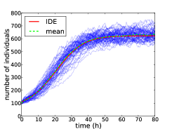
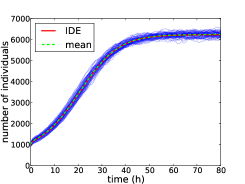
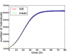
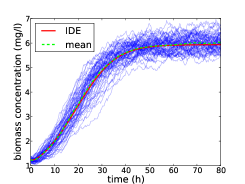
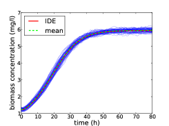
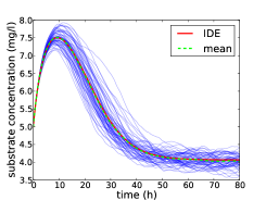
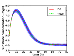
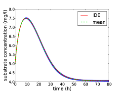
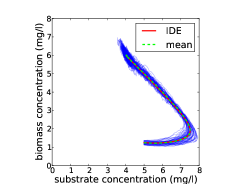
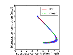
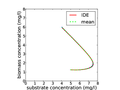
small population size	medium population size	large population size
$V=0.05$ l, $N_{0}=100$	$V=0.5$ l, $N_{0}=1000$	$V=5$ l, $N_{0}=10000$

Figure 1: From top to bottom: time evolutions of the population size, the biomass concentration, the concentration substrate and the concentrations phase portrait for the three levels of population sizes (small, medium and large). The blue curves represent the trajectories of 60 independent runs of IBM. The green curve represents the mean value of these runs. The red curve represents the solution of the IDE. The rate $D$ is 0.2 h^-1.

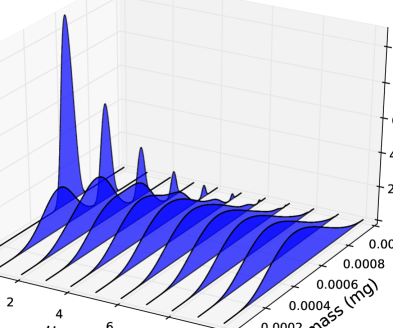
Figure 2: Time evolution of the normalized mass distribution for the IDE (33): we represent the simulation until time $T=10$ (h) only to illustrate the transient phenomenon due to the choice of the initial distribution (35). After a few iterations in time this distribution is bimodal, the upped mode growths in mass and disappears before $T=10$ (h).

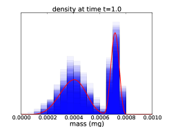
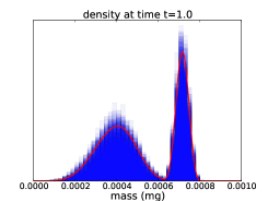
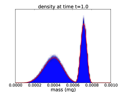
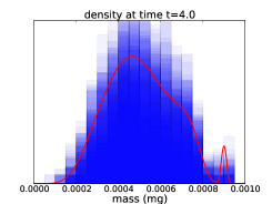
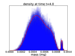
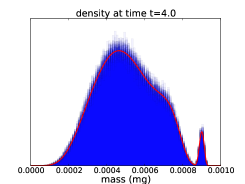
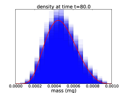
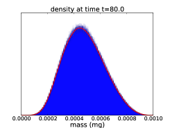
small population size	medium population size	large population size
$V=0.05$ l, $N_{0}=100$	$V=0.5$ l, $N_{0}=1000$	$V=5$ l, $N_{0}=10000$

Figure 3: Mass distribution for the time $t=1$ (above), $t=4$ (middle) and $t=80$ (bottom) in small (left), medium (middle) and large (right) population size. For each graph, the blue histograms represent the empirical mass distributions of individuals for the 60 independent runs of IBM. In order to plot the histogram we have adapted the number of bins according to the population size. The red curve represents the mass distribution given by the IDE. The dilution rate $D$ is 0.2 h^-1. Again the convergence of the IBM solution to the IDE in large population limit is observed.

6.3 Comparison of the IBM, the IDE and the ODE

We now compare the IBM and the IDE to the classical chemostat model described by the system of ODE (34). The function $\tilde{\mu}$ is the specific growth rate. The growth model in both the IBM and the IDE is of Monod type, so for the ODE model we also consider the classical Monod kinetics:

$$\tilde{\mu}(S) =\mu_{\max}\,\frac{S}{K_{s}+S}\,.$$ (36)

The parameters of this Monod law are not given in the initial model and we use a least squares method to determine the value of the parameters $\mu_{\max}$ and $K_{s}$ which minimize the quadratic distance between $(S_{t},X_{t})_{t\leq T}$ given by (34) and $(S_{t},X_{t}=\int_{\mathcal{X}}x\,p_{t}(x)\,{{\textrm{d}}}x)_{t\leq T}$ given by (32)-(33).

The numerical integration of the ODE (34) presents no difficulties and is performed by the function odeint of the module scipy.integrate of Python with the default parameters.

First we consider a simulation based on the initial mass density $d(x)$ defined by (35). With this initial density both the IDE and the IBM feature a transient phenomenon described in the previous section and illustrated in Figures (2) et (3).

Figure 4 (left) shows a significant difference between the IBM and the IDE on the one hand and the ODE on the other hand, the latter model cannot account for the transient phenomenon. With the first two models, the individual bacteria are withdrawn uniformly and independently of their mass (large mass bacteria has the same probability of withdrawal as small mass bacteria) and at the beginning of the simulation there is a decrease in biomass as at initial state $d(x)$ has a substantial proportion of large bacteria mass. The ODE is naturally not able to account for this phenomenon.

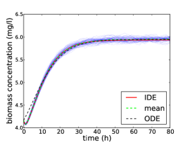
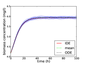
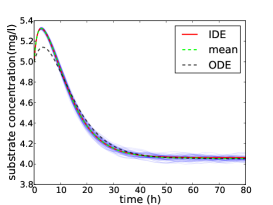
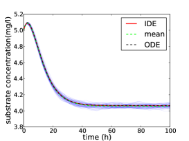
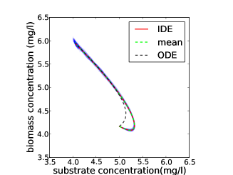
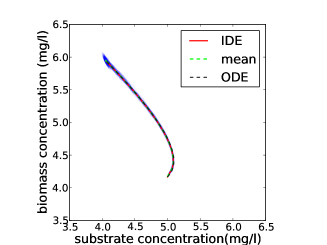
initial density $d(x)$ (35)	initial density $d^{\prime}(x)$ (37)

Figure 4: Time evolution of the biomass concentration (top), the substrate concentration (middle) and the concentration trajectories in the phase space (bottom) according to the initial mass distributions (35) (left) and (37) (right). In blue, the trajectories of 60 independent runs of the IBM simulated with $V=3$ l and $N_{0}=20000$ (left), $N_{0}=25000$ (right); in green, the mean of the IBM runs; in red, the solution of IDE (32)-(33); in black, the solution of the ODE (34). The latter is fitted by the least squares method on the IDE, the parameters of the Monod law (36) are $\mu_{\max}=0.341$ and $K_{s}=2.862$ in the first case and $\mu_{\max}=0.397$ and $K_{s}=3.996$ in the second. As initial densities are different, $N_{0}$ is adapted so that the average initial biomass concentration is the same in both cases. The dilution rate $D$ is 0.2 h^-1. In the first case, the ODE gives no account for the transient phenomenon described in the previous section, see Figures (2) and (3), while the IDE and the IBM give coherent account for it. In the second case the three models are consistent.

This phenomenon no longer appears when uses the following density:

$$d^{\prime}(x) =\Biggl{(}\frac{x-0.00035}{0.0003}\,\left(1-\frac{x-0.00035}{0.0003}\right)\Biggr{)}^{5}\,1_{\{0.00035<x<0.00065\}}\,.$$ (37)

Indeed, from Figure 4 (right), there is no longer any biomass decay at the beginning of the simulation and the different simulations are comparable, the ODE and the IDE match substantially.

6.4 Study of the washout

Figure 5: Time evolution of the biomass concentration. In blue, 1000 independent realizations of the IBM simulated with $V=0.5$ l and $N_{0}=30$; in green, the mean of these runs; in red, the solution of the IDE; in black, the solution of the ODE with parameters values $\mu_{\max}=0.482$ and $K_{s}=6.741$. The dilution rate $D$ is 0.275 h^-1. Among the 1000 independent runs of the IBM, 111 lead to washout while the deterministic models converge to an equilibrium with strictly positive biomass. The mean value of the 1000 runs of the IBM gives account for the washout probability while IDE and ODE models do not account for this question.

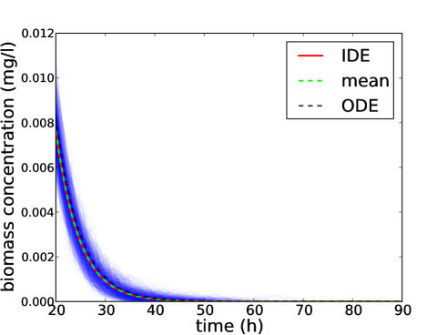
Figure 6: $\blacktriangleright$ (Top) Evolution of biomass concentration between $t=20$ and $t=90$ h: blue, 1000 independent runs of the IBM; in green, the mean value of these runs; in red the solution of the IDE; in black, the solution to the ODE with parameters $\mu_{\max}=0.814$ and $K_{s}=17.547$. The parameters are $V=10$ l and $N_{0}=10000$, the dilution rate $D$ is 0.5 h^-1. For both deterministic models, the size of the population decreases exponentially rapidly to 0 but remains strictly positive for any finite time. However, all the runs of the IBM reach washout in finite time $\blacktriangleright$ (Bottom) empirical distribution of the washout time calculated from 7000 independent runs of the IBM and plotted using a time kernel regularization.

One of the main differences between deterministic and stochastic models lies in their way of accounting for the washout phenomenon (or extinction phenomenon in the case of an ecosystem). With a sufficiently small dilution rate $D$, the solutions of the ODE (34) and the IDE (32)-(33) converge to an equilibrium point with strictly positive biomass. In fact, the washout is an unstable equilibrium point and apart from the line corresponding to the null biomass, the complete phase space corresponds to a basin of attraction leading to a solution with a strictly positive biomass asymptotic point. However, from Figure 5, among the 1000 independent runs of the IBM, 111 of them converge to washout before time $t=1000$ h; so the probability of washout at this instant is approximately 11%. It may be noted that the IDE and the ODE do not correspond to the average value of the IBM since only the latter may reflect the washout in a finite time horizon.

Now we consider a sufficiently large dilution rate, $D=0.5$ h^-1, corresponding to the washout conditions. Figure 6 (left) presents the evolution of the biomass concentration in the different models. The runs of the IBM converge to the washout in finite time whereas both deterministic ODE and IDE models converge exponentially to washout without ever reaching it in finite time. Figure 6 (right) shows the empirical distribution of the washout time calculated from 7000 independent runs of the IBM. This washout time features a relatively large variance.

Conclusion

We proposed a hybrid chemostat model. On the one hand the bacterial population is modeled as an individual-based model: each bacterium is explicitly represented through its mass. On the other hand, the substrate concentration dynamics is represented as a conventional ordinary differential equation. Mechanisms acting on the bacteria are explicitly described: growth, division and up-take. Consumption of the substrate is also described and it is through this mechanism that bacteria interact.

We described an exact Monte Carlo simulation technique of the model. Our main result is the convergence of the IBM to an integro-differential equation model when the population size tends to infinity. There is a convergence in distribution for coupled stochastic processes: the first one with càdlàg trajectories takes values ​​in the set of finite measures on the space of masses, the second one with continuous trajectories takes values ​​in the set of substrate concentration values. The integro-differential equation model limit has been known for many years as population-balance equation and is used in particular for growth-fragmentation models. The numerical tests have allowed us to illustrate this convergence: in large population, the integro-differential equation model accurately reflects the behavior of the IBM and thus, the randomness can be neglected. In small or medium population this randomness is not negligible. We also proposed a numerical test where the classical chemostat model, in terms of two coupled ordinary differential equations, cannot account for transient behavior observed with the integro-differential model as with the IBM. Finally, in the case of washout, thus in small population size, IBM gives account for the random washout time, whereas the conventional model as the integro-differential model merely offers a more limited vision of this phenomenon as an asymptotic convergence to washout, never reached in finite time.

It would be interesting to propose extensive simulations of this model, we can consider several axes. First, our simulations are based on a division rate $\lambda(s,x)$ which does not depend on the substrate concentration $s$. One can easily consider a rate depending on $s$, there are indeed such examples (see e.g. Henson,, 2003). Similarly, in our model the individual growth dynamics is deterministic, it would be appropriate to consider a stochastic individual growth dynamics. To progress in this direction it would be necessary to consider specific cases studies where more explicit growth dynamics would be specified.

It would also be pertinent to develop approximation methods based on moments, but these methods are usually ad hoc and it would be worthwhile to rely on a rigorous and systematic approach.

Finally, there are several relatively immediate extensions of the proposed model. At first, one can imagine extending the model to the case of several species and several types of substrates. One can also model the effects of aggregation of bacteria in the chemostat, for example in the form of flocculation with given rates for aggregation and fragmentation of flocs. We can also consider two classes of bacteria, attached bacteria and planktonic bacteria, to account for a biofilm dynamic.

Appendices

Appendix A Skorohod topology

The space of finite measures ${\mathcal{M}}_{F}(\mathcal{X})$ is equipped with the topology of the weak convergence, that is the smallest topology for which the applications $\zeta\to\langle\zeta,f\rangle=\int_{{\mathcal{X}}}f(x)\,\zeta({{\textrm{d}}}x)$ are continuous for any $f\in\mathcal{C}(\mathcal{X})$. This topology is metrized by the Prokhorov metric:

$$d_{\textrm{\tiny\rm PR}}(\zeta,\zeta^{\prime})\stackrel{{\scriptstyle{\textrm{\rm\tiny def}}}}{{=}}\inf\Bigl{\{}\varepsilon>0\,;\,\zeta(F)\leq\zeta^{\prime}(F^{\varepsilon})+\varepsilon\,,\$$

$$\qquad\qquad\qquad\qquad\qquad\,\,\,\zeta^{\prime}(F)\leq\zeta(F^{\varepsilon})+\varepsilon\,,\ \textrm{ for all closed }F\subset{\mathcal{X}}\Bigr{\}}$$

where $F^{\varepsilon}\stackrel{{\scriptstyle{\textrm{\rm\tiny def}}}}{{=}}\{x\in{\mathcal{X}};\inf_{y\in F}|x-y|<\varepsilon\}$ (see Daley and Vere-Jones,, 2003, Appendix A2.5). The Prokhorov distance is bounded by the distance of the total variation $d_{\textrm{\tiny\rm TV}}(\zeta,\zeta^{\prime})=\left\|\zeta-\zeta^{\prime}\right\|_{\textrm{\tiny TV}}$ associated with the norm defined by:

$$\left\|\zeta\right\|_{\textrm{\tiny TV}}\stackrel{{\scriptstyle{\textrm{\rm\tiny def}}}}{{=}}\sup_{A\in{\mathcal{B}}({\mathcal{X}})}|\zeta(A)+\zeta(A^{c})|=\zeta_{+}({\mathcal{X}})+\zeta_{-}({\mathcal{X}})=\sup_{\begin{subarray}{c}f\textrm{ continuous}\\ \left\|f\right\|_{\infty}\leq 1\end{subarray}}|\langle\zeta,f\rangle|$$

for any finite and signed measure $\zeta$ where $\zeta=\zeta_{+}-\zeta_{-}$ is the Hahn-Jordan decomposition of $\zeta$.

The space $\mathcal{D}([0,T],{\mathcal{M}}_{F}(\mathcal{X}))$ is equipped with the Skorohod metric $d_{\textrm{\tiny\rm S}}$. Instead of giving the definition of this metric (see Ethier and Kurtz,, 1986, Eq. (5.2) p. 117) we recall a characterization of the convergence for this metric.

According to the first characterization (Ethier and Kurtz,, 1986, Prop. 5.3, p. 119), a sequence $(\zeta^{n})_{n\in\mathbb{N}}$ converges to $\zeta$ in ${\mathcal{D}}([0,T],{\mathcal{M}}_{F}(\mathcal{X}))$, i.e. $d_{\textrm{\tiny\rm S}}(\zeta^{n},\zeta)\to 0$, if and only if there exists a sequence $\lambda_{n}(t)$ of time change functions such that, for all $n$, $t\to\lambda_{n}(t)$ is strictly increasing and continuous with $\lambda_{n}(0)=0$, $\lambda_{n}(t)\to_{t\to\infty}\infty$, satisfying:

$$\sup_{0\leq t\leq T}d_{\textrm{\tiny\rm PR}}({\zeta_{t}^{n},\zeta_{\lambda_{n}(t)}})\xrightarrow[n\to\infty]{}0$$ (38)

and

$$\sup_{0\leq t\leq T}|\lambda_{n}(t)-t|\to 0\,.$$ (39)

If $(\zeta^{n})_{n\in\mathbb{N}}$ converges to $\zeta$ in ${\mathcal{D}}([0,T],{\mathcal{M}}_{F}(\mathcal{X}))$ and if $\zeta\in{\mathcal{C}}([0,T],{\mathcal{M}}_{F}({\mathcal{X}}))$ then in:

$$\sup_{0\leq t\leq T}d_{\textrm{\tiny\rm PR}}(\zeta^{n}_{t},\zeta_{t})\leq\sup_{0\leq t\leq T}d_{\textrm{\tiny\rm PR}}(\zeta^{n}_{t},\zeta_{\lambda_{n}(t)})+\sup_{0\leq t\leq T}d_{\textrm{\tiny\rm PR}}(\zeta_{\lambda_{n}(t)},\zeta_{t})$$

the first term of the right-hand side tends to 0 because of (38); the second one tends to 0 because of (39) and the uniform continuity of $\zeta$ in $[0,T]$. This proves that $\zeta^{n}$ converges to $\zeta$ in ${\mathcal{D}}([0,T],{\mathcal{M}}_{F}(\mathcal{X}))$ also for the uniform metrics.

Appendix B Numerical integration scheme for the IDE

To numerically solve the system of integer-differential equations (32)-(33), that is the strong version of the limit system (23)-(24), we make use of finite difference schemes.

Given a time step $\Delta t$ and a mass step $\Delta x=L/I$, with $I\in\mathbb{N}^{*}$, we discretize the time and mass space with:

$$t_{n} =n\,\Delta t\, x_{i} =i\,\Delta x\,.$$

We introduce the following approximations:

$$p_{n,i} \simeq p_{t_{n}}(x_{i})\,, s_{n} \simeq S_{t_{n}}\,.$$

We also suppose first that at the initial time step there is no individual with null mass in the vessel, i.e. $p_{0,0}=0$; and second that individual with null mass cannot be generated during the cell division step, i.e. $q$ is regular with $q(0)=0$. This assumption was not necessary in the mathematical development presented in the previous sections but is naturally required to obtain reasonable mass of individuals in the simulation.

For time integration we use an explicit Euler scheme, for space integration, an uncentered upwind difference scheme, which leads to the coupled integration scheme:

$$\frac{p_{n+1,i}-p_{n,i}}{\Delta t} =-\rho_{\textrm{\tiny\rm\!\! g}}(s_{n},x_{i})\,\frac{p_{n,i}-p_{n,i-1}}{\Delta x}-\frac{\partial}{\partial x}\rho_{\textrm{\tiny\rm\!\! g}}(s_{n},x_{i})\,p_{n,i}$$

$$\qquad\qquad-\bigl{(}\lambda(s_{n},x_{i})+D\bigr{)}\,p_{n,i}+2\,\Delta x\,\sum_{j=1}^{I}\frac{\lambda(s_{n},x_{j})}{x_{j}}\,q\left(\frac{x_{i}}{x_{j}}\right)\,p_{n,j}\,,$$

$$\frac{s_{n+1}-s_{n}}{\Delta t} =D\,({\mathbf{s}}_{\textrm{\tiny\rm in}}-s_{n})-\frac{k}{V}\,\Delta x\,\sum_{j=1}^{I}\rho_{\textrm{\tiny\rm\!\! g}}(s_{n},x_{j})\,p_{n,j}$$

for $n\in\mathbb{N}$ and $i=1,\cdots I$, with the boundary condition:

$$p_{n+1,0}=0$$

and given initial conditions $p_{0,i}$ and $s_{0}$.

We finally get:

$$p_{n+1,i} =p_{n,i}+\Delta t\;\Biggl{\{}-\rho_{\textrm{\tiny\rm\!\! g}}(s_{n},x_{i})\,\frac{p_{n,i}-p_{n,i-1}}{\Delta x}-\frac{\partial}{\partial x}\rho_{\textrm{\tiny\rm\!\! g}}(s_{n},x_{i})\,p_{n,i}$$

$$\qquad\qquad-\bigl{(}\lambda(s_{n},x_{i})+D\bigr{)}\,p_{n,i}+2\,\Delta x\,\sum_{j=1}^{I}\frac{\lambda(s_{n},x_{j})}{x_{j}}\,q\left(\frac{x_{i}}{x_{j}}\right)\,p_{n,j}\Biggr{\}}$$

$$s_{n+1} =s_{n}+\Delta t\,\Biggl{\{}D\,({\mathbf{s}}_{\textrm{\tiny\rm in}}-s_{n})-\frac{k}{V}\,\Delta x\,\sum_{j=1}^{I}\rho_{\textrm{\tiny\rm\!\! g}}(s_{n},x_{j})\,p_{n,j}\Biggl{\}}$$

for $n\in\mathbb{N}$ and $i=1,\cdots I$ with boundary condition $p_{n+1,0}=0$ and given initial conditions $p_{0,i}$ and $s_{0}$.

References

• Allen, (2003) Allen, L. J. (2003). An Introduction to Stochastic Processes with Biology Applications. Prentice Hall.
• Billingsley, (1968) Billingsley, P. (1968). Convergence of Probability Measures. John Wiley & Sons, New York.
• Campillo et al., (2011) Campillo, F., Joannides, M., and Larramendy-Valverde, I. (2011). Stochastic modeling of the chemostat. Ecological Modelling, 222(15):2676–2689.
• Champagnat, (2006) Champagnat, N. (2006). A microscopic interpretation for adaptive dynamics trait substitution sequence models. Stochastic Processes and their Applications, 116(8):1127–1160.
• Champagnat et al., (2013) Champagnat, N., Jabin, P.-E., and Méléard, S. (2013). Adaptation in a stochastic multi-resources chemostat model. ArXiv Mathematics e-prints, arXiv:1302.0552v1 [math.PR].
• Crump and O’Young, (1979) Crump, K. S. and O’Young, W.-S. C. (1979). Some stochastic features of bacterial constant growth apparatus. Bulletin of Mathematical Biology, 41(1):53 – 66.
• Daley and Vere-Jones, (2003) D. Daley and D. Vere-Jones. An Introduction to the Theory of Point Processes – Volume I: Elementary Theory and Methods. Springer, second edition, 2003.
• Daoutidis and Henson, (2002) Daoutidis, P. and Henson, M. (2002). Dynamics and control of cell populations in continuous bioreactors. AIChE Symposium Series, 326:274–289.
• Diekmann et al., (2005) Diekmann, O., Jabin, P.-E., Mischler, S., and Perthame, B. (2005). The dynamics of adaptation: an illuminating example and a Hamilton-Jacobi approach. Theoretical Population Biology, 67(4):257–71.
• Ethier and Kurtz, (1986) Ethier, S. N. and Kurtz, T. G. (1986). Markov Processes – Characterization and Convergence. John Wiley & Sons.
• Fournier and Méléard, (2004) Fournier, N. and Méléard, S. (2004). A microscopic probabilistic description of a locally regulated population and macroscopic approximations. Annals of Applied Probability, 14(4):1880–1919.
• Fredrickson et al., (1967) Fredrickson, A., Ramkrishna, D., and Tsuchiya, H. (1967). Statistics and dynamics of procaryotic cell populations. Mathematical Biosciences, 1(3):327–374.
• Grasman et al., (2005) Grasman, J., De Gee, M., and Herwaarden, O. A. V. (2005). Breakdown of a chemostat exposed to stochastic noise volume. Journal of Engineering Mathematics, 53(3):291–300.
• Hatzis et al., (1995) Hatzis, C., Srienc, F., and Fredrickson, A. G. (1995). Multistaged corpuscular models of microbial growth: Monte Carlo simulations. Biosystems, 36(1):19–35.
• Henson, (2003) Henson, M. A. (2003). Dynamic modeling and control of yeast cell populations in continuous biochemical reactors. Computers & Chemical Engineering, 27(8-9):1185–1199.
• Hoskisson and Hobbs, (2005) Hoskisson, P. A. and Hobbs, G. (2005). Continuous culture - making a comeback? Microbiology, 151(10):3153–3159.
• Ikeda and Watanabe, (1981) Ikeda, N. and Watanabe, S. (1981). Stochastic Differential Equations and Diffusion Processes. North–Holland/Kodansha.
• Imhof and Walcher, (2005) Imhof, L. and Walcher, S. (2005). Exclusion and persistence in deterministic and stochastic chemostat models. Journal of Differential Equations, 217(1):26–53.
• Joffe and Métivier, (1986) Joffe, A. and Métivier, M. (1986). Weak convergence of sequences of semimartingales with applications to multitype branching processes. Advances in Applied Probability, 18:20–65.
• Lee et al., (2009) Lee, M. W., Vassiliadis, V. S., and Park, J. M. (2009). Individual-based and stochastic modeling of cell population dynamics considering substrate dependency. Biotechnology and Bioengineering, 103(5):891–899.
• Méléard and Roelly, (1993) Méléard, S. and Roelly, S. (1993). Sur les convergences étroite ou vague de processus à valeurs mesures. Comptes rendus de l’Académie des Sciences de Paris Sér. 1, 317:785–788.
• (22) Mirrahimi, S., Perthame, B., and Wakano, J. (2012a). Evolution of species trait through resource competition. Journal of Mathematical Biology, 64(7):1189–1223.
• (23) Mirrahimi, S., Perthame, B., and Wakano, J. Y. (2012b). Direct competition results from strong competiton for limited resource. arXiv:1201.5826v1.
• Monod, (1950) Monod, J. (1950). La technique de culture continue, théorie et applications. Annales de l’Institut Pasteur, 79(4):390–410.
• Novick and Szilard, (1950) Novick, A. and Szilard, L. (1950). Description of the chemostat. Science, 112(2920):715–716.
• Ramkrishna, (1979) Ramkrishna, D. (1979). Statistical models of cell populations. In Advances in Biochemical Engineering, volume 11, pages 1–47. Springer Berlin Heidelberg.
• Ramkrishna, (2000) Ramkrishna, D. (2000). Population Balances: Theory and Applications to Particulate Systems in Engineering. Elsevier Science.
• Roelly-Coppoletta, (1986) Roelly-Coppoletta, S. (1986). A criterion of convergence of measure-valued processes: application to measure branching processes. Stochastics, 17(1-2):43–65.
• Rüdiger and Ziglio, (2006) Rüdiger, B. and Ziglio, G. (2006). Itô formula for stochastic integrals w.r.t. compensated Poisson random measures on separable Banach spaces. Stochastics An International Journal of Probability and Stochastic Processes, 78(6):377–410.
• Smith and Waltman, (1995) Smith, H. L. and Waltman, P. E. (1995). The Theory of the Chemostat: Dynamics of Microbial Competition. Cambridge University Press.
• Stephanopoulos et al., (1979) Stephanopoulos, G., Aris, R., and Fredrickson, A. (1979). A stochastic analysis of the growth of competing microbial populations in a continuous biochemical reactor. Mathematical Biosciences, 45:99–135.
• Tran, (2006) Tran, V. C. (2006). Modèles particulaires stochastiques pour des problèmes d’évolution adaptative et pour l’approximation de solutions statistiques. PhD thesis, Université de Nanterre - Paris X.
• Tran, (2008) Tran, V. C. (2008). Large population limit and time behaviour of a stochastic particle model describing an age-structured population. ESAIM: PS, 12:345–386.