Shadow gap in the over-doped (Ba_1-xK_x)Fe₂As₂ compound

Abstract

The electron band around $M$ point in (Ba_1-xK_x)Fe₂As₂ compound – completely lifted above the Fermi level for $x>0.7$ and hence has no Fermi Surface (FS) – can still form an isotropic s-wave gap ($\Delta_{e}$) and it is the main pairing resource generating an s-wave gap ($\Delta_{h}$) with an opposite sign on the hole pocket around $\Gamma$ point. The electron band developing the SC order parameter $\Delta_{e}$ but having no FS displays a shadow gap feature which will be easily detected by various experimental probes such as angle-resolved photoemission spectroscopy (ARPES) and scanning tunneling microscope (STM). Finally, the formation of the nodal gap $\Delta_{nodal}$ with $A_{1g}$ symmetry on the other hole pocket with a larger FS is stabilized due to the balance of the interband pairing interactions from the main hole band gap $\Delta_{h}=+\Delta$ and the hidden electron band gap $\Delta_{e}=-\Delta$.

Introduction: The superconducting (SC) transition is the most well known example of the Fermi surface (FS) instability along with other density wave instabilities such as spin density wave (SDW), charge density wave (CDW), etc. Mathematically, it is summarized by a pairing susceptibility $\chi(T)=\lambda\ln{[\Lambda_{hi}/T]}$ of a conduction band of the Bloch states BCS , where $\lambda$ is a dimensionless coupling constant and $\Lambda_{hi}$ is the high energy cut-off of the pairing interaction (for example, $\Lambda_{hi}=\omega_{D}$, Debye frequency, for phonon interaction). For the conduction band with a Fermi surface (FS), the low energy cut-off is in fact zero because the presence of FS allows the zero energy excitations, which is now replaced by $T$ at finite temperature in the above formula. This susceptibility displays the logarithmic divergence with lowering temperature, hence no matter how weak the pairing interaction $\lambda$ is, the instability condition, $\chi(T)\rightarrow 1$, is achieved by decreasing temperature $T\rightarrow T_{c}=\Lambda_{hi}\exp{[-1/\lambda]}$. This is called the FS instability. However, if there exists a finite low energy cut-off $\Lambda_{low}$, for example, because there is no FS, then the susceptibility becomes $\chi\sim\lambda\ln{[\Lambda_{hi}/\Lambda_{low}]}$ and the instability condition $\chi(T)\rightarrow 1$ can only be satisfied when the coupling strength $\lambda$ becomes sufficiently strong, i.e. $\lambda>\lambda_{crit}=\frac{1}{\ln{[\Lambda_{hi}/\Lambda_{low}]}}$. This hypothetical exercise shows that the instability can still occur with Bloch states without the FS if the coupling is strong enough. However, notice that the susceptibility $\chi$ becomes temperature independent in this case, hence this mechanism cannot derive a phase transition in real system by decreasing temperature. Therefore, we confirm a common knowledge: no FS, no phase transition with Bloch states.

In this paper, however, we demonstrate that the presence of the low energy cut-off in the pairing susceptibility does not prohibit the superconducting (SC) phase transition in the multi-band SC pairing model mediated by an interband pairing interaction as most probably realized in the Fe-based superconductor Kamihara ; Stewart . In particular, in the case of the hole over-doped (Ba_1-xK_x)Fe₂As₂ compound, it is known that the electron band is completely lifted up above the Fermi level, hence the FS of the electron pocket disappears, for $x>0.7$ H Ding . In this case, we show that the SC order parameter (OP) should still be formed in the electron band, which has no FS, as well as in the hole band, maintaining the general structure of the sign-changing s-wave pairing state mediated by the antiferromagnetic (AFM) spin fluctuations.

The formation of a SC OP in the band without FS is an unprecedented SC state and its identification will be a smoking-gun evidence proving the pairing mechanism of the Iron-based superconductors mediated by the interband repulsive interactionMazin ; Kuroki ; other theory ; Bang-model . This SC gap state without FS will display a shadow gap feature in various physical properties and this shadow gap feature can be easily detected by ARPES, STM, etc. Finally, the formation of the SC pairing condensate in the electron band, although it is not visible at the Fermi level, is the main deriving force to determine the SC transition temperature $T_{c}$ and also plays an important role to stabilize a nodal SC gap in the second and/or third hole pocket with a larger FS area. Our scenario naturally explains the $T_{c}$ variation and the evolution of a nodal gap in (Ba_1-xK_x)Fe₂As₂ compound with K dopingH Ding 2 ; Avci ; S Shin ; Budko .

$T_{c}$ with the electron band lifted above Fermi level: For the purpose of demonstration, we start with a minimal two band modelBang-model : one hole band around $\Gamma$ point and one electron band around $M$ point in the folded Brillouin Zone (BZ). The pairing interaction is also assumed as a simple phenomenological form induced by the AFM spin fluctuations defined as

$$V_{AFM}(k,k^{{}^{\prime}})=V_{M}\frac{\kappa^{2}}{|(\vec{k}-\vec{k^{{}^{\prime}}})-\vec{Q}|^{2}+\kappa^{2}}.$$ (1)

where the AFM correlation wave vector $\vec{Q}$ is assumed to be $\vec{Q}=(\pi\pm\delta,\pi\pm\delta)$ to incorporate an icommensurabilityYamada . The coupled gap equations are written as

$$\Delta_{h}(k) = -\sum_{k^{{}^{\prime}}}[V_{hh}(k,k^{{}^{\prime}})\chi_{h}(k^{{}^{\prime}})\Delta_{h}(k^{{}^{\prime}})$$ (2)

$$+~{}~{}V_{he}(k,k^{{}^{\prime}})\chi_{e}(k^{{}^{\prime}})\Delta_{e}(k^{{}^{\prime}})],$$

$$\Delta_{e}(k) = -\sum_{k^{{}^{\prime}}}[V_{eh}(k,k^{{}^{\prime}})\chi_{h}(k^{{}^{\prime}})\Delta_{h}(k^{{}^{\prime}})$$ (3)

$$+~{}~{}V_{ee}(k,k^{{}^{\prime}})\chi_{e}(k^{{}^{\prime}})\Delta_{e}(k^{{}^{\prime}})].$$

where $V_{hh}(k,k^{{}^{\prime}})$, $V_{he}(k,k^{{}^{\prime}})$, etc are the interaction defined in Eq.(1) and the subscripts are written to clarify the meaning of $V_{hh}(k,k^{{}^{\prime}})$ =$V(k_{h},k^{{}^{\prime}}_{h})$, $V_{he}(k,k^{{}^{\prime}})$ =$V(k_{h},k^{{}^{\prime}}_{e})$, etc., and $k_{h}$ and $k_{e}$ specify the momentum $k$ located on the hole and electron bands, respectively. For the convenience of the analysis of $T_{c}$, we introduce the FS averaged pairing potential $<V_{he}(k,k^{{}^{\prime}})>_{FS}=V_{he}=V_{eh}$, then the coupled $T_{c}$-equations are written as

$$\Delta_{h} = -\bigl{[}V_{hh}N_{h}\chi_{h}\bigr{]}\Delta_{h}-\bigl{[}V_{he}N_{e}\chi_{e}\bigr{]}\Delta_{e},$$ (4)

$$\Delta_{e} = -\bigl{[}V_{ee}N_{e}\chi_{e}\bigr{]}\Delta_{e}-\bigl{[}V_{eh}N_{h}\chi_{h}\bigr{]}\Delta_{h}.$$

where the pair susceptibility is defined as

$$\chi_{h,e}(T) = \int_{0}^{\Lambda_{hi}}\frac{d\xi}{\xi}\tanh(\frac{\xi}{2T})\approx\ln\Big{[}\frac{1.14\Lambda_{hi}}{T}\Big{]},$$ (5)

and $N_{h,e}$ are the density of states (DOS) of the hole band and electron band, respectively. For simplicity of demonstrating the mechanism, we temporarily drop the intraband interaction $V_{hh}$ and $V_{ee}$, which are always much weaker than $V_{he}=V_{he}$. Then the gap equations can be combined to be

$$\Delta_{h} = \bigl{[}V_{he}N_{e}\chi_{e}\bigr{]}\cdot\bigl{[}V_{eh}N_{h}\chi_{h}\bigr{]}\Delta_{h},$$ (6)

$$\approx \bigl{[}V_{he}N_{e}V_{eh}N_{h}\bigr{]}\Big{[}\ln\big{(}\frac{1.14\Lambda_{hi}}{T}\big{)}\Big{]}^{2}\Delta_{h},$$ (7)

hence we can read off the critical temperature

$$T_{c0}\approx 1.14\Lambda_{hi}\exp{\big{[}-\frac{1}{\lambda_{eff}}\big{]}}$$ (8)

with $\lambda_{eff}=\sqrt{V_{he}N_{e}V_{eh}N_{h}}$. Now if the electron band does not cross the Fermi level and the bottom of the band is above the Fermi level by $\epsilon_{b}$, the only modification note 2 of the above analysis is to replace the susceptibility of the electron band as follows

$$\chi_{e}=\int_{\epsilon_{b}}^{\Lambda_{hi}}\frac{d\xi}{\xi}\tanh(\frac{\xi}{2T})\approx\ln\Big{[}\frac{1.14\Lambda_{hi}}{\epsilon_{b}}\Big{]},$$ (9)

so that the coupled susceptibility in Eq.(7) changes from $\Big{[}\ln\big{(}\frac{1.14\Lambda_{hi}}{T}\big{)}\Big{]}^{2}$ to $\Big{[}\ln\big{(}\frac{1.14\Lambda_{hi}}{T}\big{)}\Big{]}\Big{[}\ln\big{(}\frac{1.14\Lambda_{hi}}{\epsilon_{b}}\big{)}\Big{]}$ and then,

$$T_{c}(\epsilon_{b})\approx 1.14\Lambda_{hi}\exp{(-1/\tilde{\lambda}_{eff})}$$ (10)

with $\tilde{\lambda}_{eff}=[V_{he}N_{e}V_{eh}N_{h}]\cdot\ln\Big{[}\frac{1.14\Lambda_{hi}}{\epsilon_{b}}\Big{]}$. Notice that this analysis is accurate only when $\epsilon_{b}>T_{c0}$, that is the same condition as $\ln\Big{[}\frac{1.14\Lambda_{hi}}{\epsilon_{b}}\Big{]}<1$. In the other limit the susceptibility of the electron band $\chi_{e}$ of Eq.(9) should be numerically calculated. Nevertheless the above analysis and Eq.(10) clearly demonstrate the fact that in the multiband pairing model mediated by the interband interaction the FS instability still operates even if the FS of the electron band disappears and the $T_{c}(\epsilon_{b})$ will only continuously decrease as the bottom of the electron band $\epsilon_{b}$ is lifted up above the Fermi level.

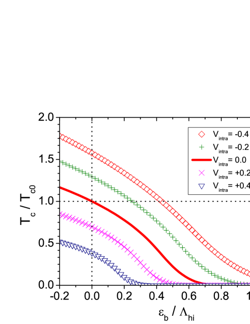
Figure 1: (Color online) Numerically calculated $T_{c}$ of the two band model vs the bottom of the electron band $\epsilon_{b}$ for different values of the intra-band interaction $V_{intra}/V_{inter}=-0.4,-0.2,0.0,+0.2,$ and $+0.4$. $T_{c}$ values are normalized by $T_{c0}(V_{intra}=0.0,\epsilon_{b}=0.0)$. We assumed a repulsive interaction for $V_{inter}=V_{he}=V_{eh}>0$ but considered both repulsive and attractive interactions for $V_{intra}$. For simplicity but without loss of generality, we also chose $N_{h}=N_{e}$ and $V_{intra}=V_{ee}=V_{hh}$.

In Fig.1, we show the numerical results of the exact $T_{c}(\epsilon_{b})$ calculated with Eq.(2) and Eq.(3) including both interband interaction ($V_{eh}$) and intraband interactions ($V_{ee}$ and $V_{eh}$). The positive $\epsilon_{b}>0$ value is the distance of the bottom of the electron band above the Fermi level; therefore no FS exists for the electron band. The negative $\epsilon_{b}<0$ value means that the electron band slightly sinks below the Fermi level, hence has a small FS. We assumed the repulsive inter-band interaction $V_{inter}=V_{eh}=V_{he}>0$ to induce the $\Delta_{\pm}$ gap solutionBang-model . However, for the intra-band interaction, we considered both repulsive and attractive interaction for generality. The attractive intra-band interaction can be possibly caused by phonons Bang-phonon or by the orbital fluctuationsKontani . The overall behavior of $T_{c}(\epsilon_{b})$ as a function of $\epsilon_{b}$ is similar for all cases; linear decrease for small $\epsilon_{b}$ value and then exponential decrease for large $\epsilon_{b}$ value in accord with Eq.(10). This behavior is qualitatively in agreement with the $T_{c}$ variation with K doping of (Ba_1-xK_x)Fe₂As₂ compoundH Ding 2 ; Avci ; S Shin ; Budko and we can understand that the main reason of the decrease of $T_{c}$ in (Ba_1-xK_x)Fe₂As₂ compound is the lifting of the bottom of the electron band $\epsilon_{b}$ with K doping. Furthermore it shows that even when $\epsilon_{b}$ is lifted up above the Fermi level and hence the FS of the electron band completely disappears, the pairing mechanism mediated by the repulsive interband scattering $V_{inter}$ between the hole and electron bands continues to operate. When the intra-band interaction $V_{intra}$ is sufficiently attractive (the case $V_{intra}=-0.4V_{inter}$ in Fig.1), the $T_{c}$ finally converges to the limit where the only the hole band forms a SC transition with the attractive interaction.

Shadow Gap of the electron band: Here we solved the coupled gap equations Eq.(2) and Eq.(3) with the realistic tight binding bands Bang-model and the fully momentum dependent phenomenological pairing interaction of Eq.(1). Although it is not crucial for the results of this paper in the following, we also employed the incommensurability ($\delta=0.32\pi$) of the spin fluctuations which is recently measured by the neutron experiment in KFe₂As₂ by Yamada and coworkers Yamada . We used two model bands: $\epsilon_{h}(k)=t_{1}^{h}(\cos k_{x}+\cos k_{y})+t_{2}^{h}\cos k_{x}\cos k_{y}+\epsilon_{h}$ and $\epsilon_{e}(k)=t_{1}^{e}(\cos k_{x}+\cos k_{y})+t_{2}^{e}\cos\frac{k_{x}}{2}\cos\frac{k_{y}}{2}+\epsilon_{e}$ with the band parameters as (0.30,0.24,-0.6) for hole band and (1.14,0.74,$\epsilon_{e}$) for electron band with the notation ($t_{1},t_{2},\epsilon$). The electron bands located in the $M$ points ($(\pi,\pi)$ in the folded BZ) is artificially lifted by shifting the parameter $\epsilon_{e}$. For example, we need $\epsilon_{e}=2.28$ to set $\epsilon_{b}=0.0$ which is the case when the bottom of the electron band just touches the Fermi level. With these parameters, the DOS of hole band near FS $N_{h}(0)$ and the DOS of the electron band near the bottom $N_{e}(0)$ are $\sim 0.45/eV$ and $\sim 0.19/eV$, respectively. Other parameters such as the coupling strength and the pairing cut-off energy $\omega_{AFM}$, etc need not be accurate since all results are renormalized by the gap values. With the above parameters, the ratio of gap sizes is $|\Delta_{e}|/|\Delta_{h}|\sim 3.4$.

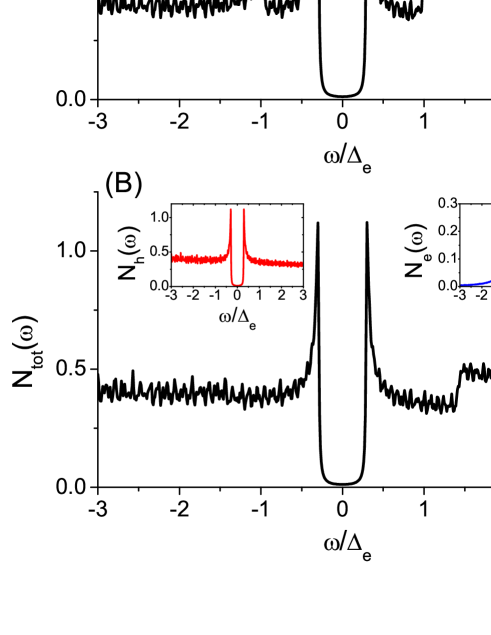
Figure 2: (Color online) Calculated density of states, $N_{h}(\omega)$, $N_{e}(\omega)$, and the total $N_{total}(\omega)$ of the two band model in the SC state. (A) is the case of $\epsilon_{b}=0.0$ and (B) is the case of $\epsilon_{b}=|\Delta_{e}|$.

In Fig.2, we show the calculated DOSs, $N_{h}(\omega)$, $N_{e}(\omega)$, and the total $N_{total}(\omega)$. Figure 2.(A) is the case when $\epsilon_{b}=0.0$. The electron band exists only above the Fermi level. Nevertheless, in the SC state, the Bogoliubov quasiparticles are formed above and below the Fermi level, hence the DOS $N_{e}(\omega)$ is created both for $\omega>0$ and for $\omega<0$. However, the shape of $N_{e}(\omega)$ is very asymmetric for above and below $\omega=0$ as seen in the right inset of Fig.2(A). It should be contrasted with $N_{h}(\omega)$ in the left inset which is symmetric as a typical SC DOS. The total DOS $N_{total}(\omega)$ displays this clear signature of the asymmetric DOS due to the shadow gap formed in the electron band above the Fermi level. Fig.2(B) is the case $\epsilon_{b}=|\Delta_{e}|$. In this case the gap size in $N_{e}(\omega)$ becomes $\sqrt{\epsilon_{b}^{2}+\Delta_{e}^{2}}$ and the shapes of $N_{e}(\omega)$ and $N_{tot}(\omega)$ become even more asymmetric than the $\epsilon_{b}=0$ case. This predicted asymmetric DOS should be easily detected by the STM measurement.

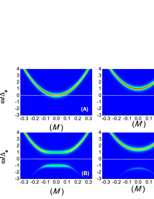
Figure 3: (Color online) The quasiparticle spectral density of the electron band $\epsilon_{e}(k)$ near the $M$ point. (A) and (B) are the normal state and the SC state of the case $\epsilon_{b}=0.0$, respectively. (C) and (D) are the corresponding results of the case $\epsilon_{b}=|\Delta_{e}|$.

In Fig.3, we showed the one particle spectral density of the electron band near the $M$ point. This is calculated by $\frac{1}{\pi}ImG_{e}(\omega,k)=\frac{1}{\pi}Im\frac{\omega+\epsilon_{e}(k)}{\omega^{2}-[\epsilon_{e}^{2}(k)+\Delta_{e}^{2}]}$. These results are another manifestation of the shadow gap feature of the electron band which does not have the FS. Fig.3(A) and (B) are the normal state and the SC state of the case $\epsilon_{b}=0.0$, respectively, and Fig.3(C) and (D) are the corresponding results of the case $\epsilon_{b}=|\Delta_{e}|$. In the normal state, the quasiparticles do not appear below the Fermi level simply because the band does not exist there. However, when temperature decreases below $T_{c}$, the quasiparticle spectral density appears below the Fermi level. This dramatic effect should be easy to be detected by the ARPES measurement and in fact it seems already detected in other Iron-based superconducting compound FeTe_0.6Se_0.4 by Shin and coworkers BCS-BEC although the interpretation of the authors BCS-BEC is somewhat different than ours.

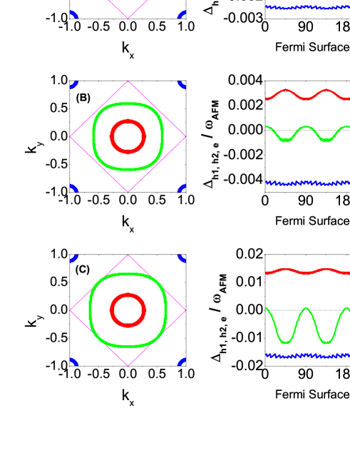
Figure 4: (Color online) (Left panel) The FS evolution of three band model; only the $h2$-band (green line) varies and the $e$-band FS is only for showing and in real calculations it has zero size with $\epsilon_{b}=0$. (Right panel) The corresponding gap solutions $\Delta_{h1}$ (red line), $\Delta_{h2}$ (green line), $\Delta_{e}$ (blue line), respectively.

Evolution of nodal gap in (Ba_1-xK_x)Fe₂As₂: The end member of (Ba_1-xK_x)Fe₂As₂ compound, KFe₂As₂, has been considered as the most strong candidate for a nodal gap superconductor among the Iron-based superconductors K122-nodal . And the optimal doped Ba_0.6K_0.4Fe₂As₂ is well confirmed to have the isotropic full s-wave gaps Stewart ; optimal . Therefore the evolution from a full gap to a nodal gap in (Ba_1-xK_x)Fe₂As₂ compound has been a keen interest in the past years H Ding 2 ; Avci ; S Shin ; Budko .

In this section, in order to study the gap evolution in (Ba_1-xK_x)Fe₂As₂, we introduce the minimal three band model. In particular, we focus on the relation between the FS size and the anisotropic gap or nodal gap evolution. We add one more hole band $\epsilon_{h2}(k)=t_{1}^{h2}(\cos k_{x}+\cos k_{y})+t_{2}^{h2}\cos k_{x}\cos k_{y}+t_{3}^{h3}(\cos 2k_{x}+\cos 2k_{y})+\epsilon_{h2}$ to the previous studied two band model, so that we have two hole bands $h1$ and $h2$ and one electron band $e$. The second hole band $h2$ is tuned to have a larger FS than the one of $h1$-band; we used parameters $(0.7,-0.1,0.3,\epsilon_{h2})$ and varied $\epsilon_{h2}$ to change the FS size. For systematic study of the FS evolution, we fix the sizes of the FS of $h1$-band and $e$-band. In the case of $e$-band, in fact, we chose to have $\epsilon_{b}=0$, i.e. the FS size of $e$-band is zero. The spin fluctuation interaction $V_{AFM}({\bf q})$ given by Eq.(1) is also fixed with $\kappa=0.3\pi$ and $\delta=0.32\pi$.

In Fig.4, we showed the gap solutions for the several different size of the $h2$-hole pocket. In the left panel, the FSs of three bands are drawn for different values of $\epsilon_{h2}$ in the folded BZ. As said above, $h1$-band and $e$-band are fixed while only the FS size of $h2$-band varies. Also the $e$-band pocket is drawn only for showing but in real calculations its size is zero because we chose $\epsilon_{b}=0$. As expected, when the $h2$-hole pocket is close to the $h1$-hole pocket as in Fig.4(A), the gap solution is basically a $\pm$s-wave state: the hole bands have all $+\Delta$ and electron band has all $-\Delta$ despite some degree of anisotropy. The degree of anisotropy is determined by the sharpness of the pairing interaction $V_{AFM}({\bf q})$ in momentum space, which is determined by $\kappa\sim\xi^{-1}$, and the FS sizes. The reason why the average sign of $h2$-band gap is ”$+$” is because the distance between $h2$-band pocket and $e$-band pocket in the BZ is closer to $(\pi\pm\delta,\pi\pm\delta)$ than what the distance between $h2$-band pocket and $h1$-band pocket is to $(\pi\pm\delta,\pi\pm\delta)$.

With increasing the $h2$-pocket, the $h2$-band gap $\Delta_{h2}$ obtains the ”$+$” section and ”$-$” section, hence becomes a nodal gap with $A_{1g}$ symmetry. In our simple toy model with a simple phenomenological interaction Eq.(1) between all bands – both intra and inter – and without any orbital degrees of freedom, this dramatic gap evolution only with a small increase of the FS size, fixing all other parameters, is demonstrating that the subtle balance of the repulsive and attractive interactions between bands is the crucial mechanism to induce and stabilize the nodal gap solution. In the case of Fig.4(B), both $+\Delta$ gap of the $h1$-band and $-\Delta$ gap of the $e$-band exert a similar strength of the repulsive and attractive interactions, respectively, to the $h2$-band from the same $V_{AFM}({\bf q})$. Therefore the $h2$-band should maximize the condensation energy gain by properly distributing $+$ OP and $-$ OP, hence developing accidental nodes but keeping $A_{1g}$ symmetry because of the crystal symmetry. Further increasing the $h2$-pocket size in Fig.4(C), the average repulsive interaction from the $h1$-band is larger than the average attractive interaction from the $e$-band, hence $\Delta_{h2}$ develops more negative lobes; here the average interactions $<V_{AFM}({\bf q})>_{h1,h2}$ and $<V_{AFM}({\bf q})>_{e,h2}$ depend on the weighting of DOSs $N_{h1}$, $N_{h2}$ and $N_{e}$ and the average ${\bf q}$ value in comparison to $(\pi\pm\delta,\pi\pm\delta)$.

Assuming that the $h2$-pocket size increases in (Ba_1-xK_x)Fe₂As₂ with the K doping, the overall gap anisotropy of the $h2$-band and the systematic development of the nodal gap structure shown in Fig.4 is surprisingly consistent with the recent ARPES observation by Shin and coworkersShin-2 . Our $h2$-band should be compared to the outer hole band and our $h1$-band represents the inner and middle bands in Ref.Shin-2 . Of course, there is a discrepancy, that is, the overall gap size(s) increases with the $h2$-pocket size in our calculations which is clearly opposite to the experimental observation. However, in our calculations in Fig.4, we fixed the $\epsilon_{b}$ and $V_{AFM}({\bf q})$ both of which should change with K doping in (Ba_1-xK_x)Fe₂As₂ toward the direction reducing $T_{c}$ and the gap sizes, so that this discrepancy can naturally be cured with a more realistic model.

Conclusion: We showed that the absence of the FS does not ruin the FS instability of the SC transition in the multi-band pairing model mediated by the interband scattering. We demonstrated that the $T_{c}$ evolution with the bottom of the electron band $\epsilon_{b}$ can consistently explain the experimental $T_{c}$ evolution of (Ba_1-xK_x)Fe₂As₂ compound. As a smoking-gun evidence of this hidden band pairing proposed in this paper, we predicted the shadow gap features both in ARPES and STM measurements. Finally, we demonstrated that the hidden electron band should continue to play an crucial role for the pairing mechanism as well as the nodal gap development in (Ba_1-xK_x)Fe₂As₂ compound.

Acknowledgement – This work was supported by Grants No. NRF-2011-0017079 funded by the National Research Foundation of Korea.

References

- (1) J. Bardeen, L. N. Cooper, and J. R. Schrieffer, Phys. Rev. 108, 1175 (1957).
- (2) Y. Kamihara et al., J. Am. Chem. Soc., 130, 3296 (2008); G. F. Chen, Z. Li, D. Wu, G. Li, W.Z. Hu, J. Dong, P. Zheng, J.L. Luo, N.L. Wang, Phys. Rev. Lett. 100, 247002 (2008); X. H. Chen, T. Wu, G. Wu, R. Liu, H. Chen, and D. Fang, Nature (London) 453, 761 (2008).
- (3) G. R. Stewart, Rev. Mod. Phys. 83, 1589 (2011).
- (4) T. Sato, K. Nakayama, Y. Sekiba, P. Richard, Y.-M. Xu, S. Souma, T. Takahashi, G. F. Chen, J. L. Luo, N. L. Wang, and H. Ding, Phys. Rev. Lett. 103, 047002 (2009).
- (5) K. Kuroki, S. Onari, R. Arita, H. Usui, Y. Tanaka, H. Kontani, and H. Aoki , Phys. Rev. Lett. 101, 087004 (2008);
- (6) I.I. Mazin, D.J. Singh, M.D. Johannes, M.H. Du, Phys. Rev. Lett. 101, 057003 (2008).
- (7) P. J. Hirschfeld, M. M. Korshunov, I. I. Mazin, Rep. Prog. Phys. 74, 124508 (2011).
- (8) Y. Bang and H.-Y. Choi, Phys. Rev. B, 78, 134523 (2008).
- (9) K. Nakayama et al., Phys. Rev. B 83, 020501(R) (2011).
- (10) Avci et al., Phys. Rev. B 85, 184507 (2012).
- (11) S. L. Bud’ko, M. Sturza, D. Y. Chung, M. G. Kanatzidis, P. C. Canfield, arXiv:1303.2010 (unpublished).
- (12) K. Okazaki et al., Science 337, 1314 (2012).
- (13) C. H. Lee et al., Phys. Rev. Lett. 106, 067003 (2011).
- (14) It is a good approximation that the DOS near the bottom of the electron band is a constant because the band has a quasi two dimensional parabolic dispersion.
- (15) Y. Bang, Phys. Rev. B 79, 092503 (2009).
- (16) H. Kontani and S. Onari Phys. Rev. Lett. 104, 157001 (2010).
- (17) K. Okazaki et al., arXiv:1307.7845 (unpublished).
- (18) K. Hashimoto et al., Phys. Rev. B, 82 014526 (2010); J. K. Dong et al., Phys. Rev. Lett. 104, 087005 (2010); J.-Ph. Reid et al., Phys. Rev. Lett. 109, 087001 (2012); Y. Bang, Supercond. Sci. Technol. 25, 084002 (2012).
- (19) G. Mu, H. Luo, Z. Wang, L. Shan, C. Ren, and Hai-Hu Wen, Phys. Rev. B 79, 174501 (2009).
- (20) Y. Ota et al., arXiv:1307.7922 (unpublished).