Tunable non-Gaussian resources for continuous-variable quantum technologies

Abstract

We introduce and discuss a set of tunable two-mode states of continuous-variable systems, as well as an efficient scheme for their experimental generation. This novel class of tunable entangled resources is defined by a general ansatz depending on two experimentally adjustable parameters. It is very ample and flexible as it encompasses Gaussian as well as non-Gaussian states. The latter include, among others, known states such as squeezed number states and de-Gaussified photon-added and photon-subtracted squeezed states, the latter being the most efficient non-Gaussian resources currently available in the laboratory. Moreover, it contains the classes of squeezed Bell states and even more general non-Gaussian resources that can be optimized according to the specific quantum technological task that needs to be realized. The proposed experimental scheme exploits linear optical operations and photon detections performed on a pair of uncorrelated two–mode Gaussian squeezed states. The desired non-Gaussian state is then realized via ancillary squeezing and conditioning. Two independent, freely tunable experimental parameters can be exploited to generate different states and to optimize the performance in implementing a given quantum protocol. As a concrete instance, we analyze in detail the performance of different states considered as resources for the realization of quantum teleportation in realistic conditions. For the fidelity of teleportation of an unknown coherent state, we show that the resources associated to the optimized parameters outperform, in a significant range of experimental values, both Gaussian twin beams and photon-subtracted squeezed states.

I Introduction

Quantum information with Gaussian states of continuous variable systems has been investigated thoroughly and with startling success both theoretically and experimentally (for comprehensive reviews of different aspects see, e.g., Refs. Adesso2007 ; Braunstein2005 ; Kok2007 ; Eisert2003 ; Dellanno2006 ). At the same time, there has been growing awareness of some important limitations intrinsic to working entirely within the framework of Gaussian states and/or Gaussian operations, so that at some point it becomes both desirable and necessary to start exploring the vast ocean of continuous-variable non-Gaussian states and non-Gaussian operations. The first pioneering and paradigmatic example of this need is given by the by now classic proof that distillation of Gaussian entangled states resorting only to Gaussian operations is impossible Scheel2002 .

In fact, various compelling reasons suggest a thorough investigation of the properties of continuous-variable non-Gaussian states. Gaussian states are indeed extremal in the sense that at fixed covariance matrix several nonclassical properties such as entanglement, when measured by the entanglement of formation, and distillable secret key rates are minimized by Gaussian states Wolf2006 . Specific families of non-Gaussian entangled resources lead to significant improvements in the performance of existing continuous-variable quantum information protocols such as teleportation Dellanno2007 ; Dellanno2010 . Measurement-based quantum computation with continuous variables eventually needs both non-Gaussian operations and non-Gaussian resource states in order to be universal Ohliger2010 ; Ohliger2012 . Preliminary investigations of the interplay of non-Gaussian inputs and different types of Gaussian and non-Gaussian channels unveils the clear advantages, in general, of non-Gaussianity for state estimation and metrology Adesso2009 ; Monras2010 ; Monras2011 ; Datta2012 ; Genoni2013 . Stronger violations of Bell inequalities and better performing entanglement swapping protocols are also expected using non-Gaussian resources and strategies beyond the currently available ones Obermaier2011 ; Banaszek1999 ; Son2009 ; Sciarrino2012 ; Sciarrino2013 . While so-called Gaussifier protocols of entanglement distillation have been proposed that convert noisy non-Gaussian states into Gaussian ones through converging iterative procedures Distillery2012 ; Campbell2013 , general optimal strategies for the distillation of highly entangled non-Gaussian states are still lacking. Finally, the interplay of non-Gaussianity, non-classicality, and non-Markovianity is expected to lead to further new phenomena when addressing the dynamics of open continuous-variable systems.

Among the many families of continuous-variable non-Gaussian states that can be of interest for fundamental quantum physics as well as for quantum information and related quantum technologies one should mention squeezed cat states Dellanno2006 ; multiphoton squeezed states, that is states that generalize the usual two-photon Gaussian squeezed states by considering nonlinear extensions of the linear Bogoliubov squeezing transformations, either single-mode Dellanno2004 or two-mode Dellanno2004bis ; and especially squeezed Bell states Dellanno2007 . Indeed, the latter include squeezed Fock and de-Gaussified squeezed coherent states as particular cases, as we shall review below. Non-Gaussian and De-Gaussified states can be generated either by introducing higher-order nonlinearities in the source, and/or by performing conditional measurements.

Many theoretical and experimental efforts have been concentrated on the engineering of nonclassical, non-Gaussian states of the radiation field Za ; We ; Ta ; Our ; Lv ; Da ; dauria05 . In particular, concerning quantum teleportation with continuous variables Vaidman ; BrauKimb ; Furusawa98 ; Lee11 , it has been demonstrated that the fidelity of teleportation can be improved using various families of non-Gaussian resources Opa ; Co ; Oli . At present, the best experimentally realized non-Gaussian resource for continuous-variable teleportation is the photon-subtracted squeezed state We ; Ta ; Our . On the other hand, as already mentioned, a new class of continuous-variable non-Gaussian states, the Squeezed Bell states, has been introduced recently Dellanno2007 . These states interpolate between different de-Gaussified states, and can be fine tuned by acting on an independent free parameter in addition to the squeezing.

From a theoretical point of view, entangled Gaussian and de-Gaussified states are defined by applying squeezing and ladder operators on the two-mode vacuum. Within this theoretical context the teleportation fidelity for the Braunstein-Kimble-Vaidman protocol is improved, in a significant range of the parameters, by replacing Gaussian and de-Gaussified resources by optimized squeezed Bell states Dellanno2007 . This has been verified for different inputs (including coherent states, squeezed states, and squeezed number states), also in the presence of losses and other realistic sources of imperfections Dellanno2010 . This effect can be understood by remarking a crucial difference existing between the case of teleportation protocols relying on entangled Gaussian resources and the case allowing for more general entangled states. In the former it is known that the fidelity of teleportation and the entanglement of the shared entangled Gaussian resource are in one-to-one correspondence Adesso2005 . In the latter this is no longer true and the fidelity of teleportation becomes a highly complicated function of three (in general conflicting) variables: degree of entanglement, degree of non-Gaussianity, and degree of Gaussian affinity Dellanno2007 . In particular, the third variable (Gaussian affinity) is crucial. It quantifies the overlap with the two-mode squeezed vacuum. Loosely speaking, it assures that an efficient entangled resource must contain a contribution, with a relevant weight, given by the two-mode squeezed vacuum plus symmetric non Gaussian corrections. The optimized squeezed Bell states realize indeed the best possible compromise for the simultaneous maximization over all these three properties of the fidelity of teleportation Dellanno2007 .

Going beyond these preliminary theoretical results, the desired goal would be to construct experimental platforms capable of generating classes of highly tunable non-Gaussian resources with enhanced performances for protocols of quantum technology based on continuous variables. In order to proceed towards concrete experimental realizations, one needs to introduce a basic scheme of generation that takes into account all the relevant sources of noise and imperfections in realistic instances. Thereafter, one must verify that in these realistic scenarios the performance of the new resource in the framework of a given quantum protocol provides an appreciable advancement that justifies the experimental effort. After this preliminary analysis, one needs to work out carefully the details of the experimental setup and, finally, one needs to provide reliable methods for the reconstruction of the experimentally generated states.

In the present work we introduce the basic scheme of generation for a large class of tunable two-mode entangled non-Gaussian states and we present a preliminary analysis on their performance as resources for continuous-variable quantum technologies. The experimental scheme that we are going to introduce has the advantage of being flexible and versatile, in the sense that a variation of the freely adjustable experimental parameters allows for the generation of different non-Gaussian states including, besides the squeezed Bell states, photon-added squeezed states Li02 , photon-subtracted squeezed states Ta , squeezed number states and, obviously, also Gaussian twin beams dauria09 ; Buono10 . The relative performance of different states will will be investigated in detail for the protocol of quantum teleportation of unknown coherent states Vaidman ; BrauKimb . We will show that the optimized states in realistic conditions provide, in a significant range of physical parameters, a superior performance compared to all existing de-Gaussified states.

II Experimental scheme with adjustable free parameters for the generation of non-Gaussian states

The pure (normalized) squeezed Bell states originally introduced in Refs. Dellanno2007 ; Dellanno2010 are of the form

$$|\Psi>_{\text{{SB}}}\equiv S_{12}\left(-r\right)\left\{\cos\delta|0,0>_{12}+\sin\delta|1,1>_{12}\right\}\;,$$ (1)

where $|0,0>_{12}$ and $|1,1>_{12}$ denote, respectively, the tensor product of two single-mode vacua and two one-photon states, while $S_{ij}\left(-r\right)=\exp\left\{ra_{i}^{{\dagger}}a_{j}^{{\dagger}}-ra_{i}a_{j}\right\}$ is the two-mode squeezing operator, and $\delta$ is a free parameter allowing for optimization. A more general form of the squeezed Bell states could include a relative phase, but this inclusion would not improve the performance of the squeeze Bell states when considered as entangled resources. At some suitably chosen values of the $\delta$ parameter, the squeezed Bell superposition coincides with de-Gaussified photon-added states, photon-subtracted states, with squeezed number states, and with Gaussian twin beams Dellanno2007 , where addition/subtraction operations, as well as the number state, are referred to the case of a single photon. For a reminder, we list in Table 1 the theoretical definitions of all the states considered.

State	Definition
Photon-subtracted squeezed state	$N_{PS}\;a_{1}a_{2}S_{12}(\zeta)|0,0>_{12}$
Photon-added squeezed state	$N_{PA}\;a_{1}^{\dagger}a_{2}^{\dagger}S_{12}(\zeta)|0,0>_{12}$
Squeezed number state	$S_{12}(\zeta)|1,1>_{12}$
Gaussian twin beam	$S_{12}(\zeta)|0,0>_{12}$

Table 1: Theoretical definition of some states of particular interest that are included in the class of squeezed Bell states. $N_{PS}$ and $N_{PA}$ denote, respectively, the normalization of de-Gaussified photon-subtracted and photon-added squeezed states.

In this section we introduce a scheme capable to generate two-mode non-Gaussian states of the electromagnetic field that provide the best experimental approximation to the form and/or to the performance of the theoretically defined squeezed Bell states. The idea is to manipulate an overall four-mode system described by two independent Gaussian twin beams, one of which will play the role of an ancillary two-mode state, and then exploit linear optical components and conditional measurements. In this respect, we recall that twin beams are routinely generated in type II Optical Parametric Oscillators (OPOs) Fornaro08 . Therefore, in our scheme, no higher-order nonlinearities are either needed or desirable. The basic generation scheme is illustrated in Fig. (1).

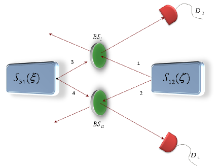
Figure 1: Sketch of the ideal scheme for the experimental generation of the states defined theoretically in Eq. (4). Two Gaussian twin beams, generated independently, respectively $\left|\zeta\right\rangle_{12}$ and $\left|\xi\right\rangle_{34}$, impinge on two beam splitters $BS_{I}$ and $BS_{II}$ of transmissivity $T_{1}$ and $T_{2}$. The generation of the output two-mode state is triggered by two simultaneous detections realized by the single-photon projective detectors $D_{3}$ and $D_{4}$.

In this scheme we exploit two independent Gaussian twin beams, $|\zeta>_{12}=S_{12}(\zeta)|0,0>_{12}$ and $|\xi>_{34}=S_{34}(\xi)|0,0>_{34}$, so that we start with an initial four-mode ”proto-state”

$$|\zeta>_{12}|\xi>_{34}=S_{12}(\zeta)S_{34}(\xi)|\mathbf{0}>_{1234}\;,$$ (2)

where $|\mathbf{0}>_{1...n}=\bigotimes\nolimits_{k=1}^{n}|0>_{k}$ denotes the tensor product of $n$ single-mode vacuum states. The twin beams feed the input ports of two beam splitters, respectively of transmissivity $T_{1}$ and $T_{2}$. Modes $1,3$ mix at the beam splitter $BS_{I}$, while modes $2,4$ mix at the beam splitter $BS_{II}$. The resulting state is a four-mode entangled state $|\Phi>_{1234}$ of the form

$$|\Phi>_{1234}=U_{13}(\kappa_{1})U_{24}(\kappa_{2})|\zeta>_{12}|\xi>_{34}$$ (3)

$$= U_{13}(\kappa_{1})U_{24}(\kappa_{2})S_{12}(\zeta)S_{34}(\xi)|\mathbf{0}>_{1234}\,,$$

where $S_{12}(\zeta)$ and $S_{34}(\xi)$ are the squeezing operators with complex squeezing parameters $\zeta=r\exp\left\{i~{}\phi_{\zeta}\right\}$ and $\xi=s\exp\left\{i~{}\phi_{\xi}\right\}$ respectively. The beam splitter operators read $U_{lk}(\kappa_{l})=\exp\left\{\kappa_{l}\left(a_{l}^{{\dagger}}a_{k}-a_{l}a_{k}^{{\dagger}}\right)\right\}$, where $l=1,k=2$ for the first beam splitter, and $l=3,k=4$ for the second one. Finally, $\tan\kappa_{l}=\sqrt{\left(1-T_{l}\right)/T_{l}}$.

Starting with the four-mode state $|\Phi>_{1234}$, the conditional measurements provided by the simultaneous clicks of the detectors $D_{3},D_{4}$, and the restriction to suitable ranges of the beam splitters parameters and of the squeezing parameters, will lead to the generation of two-mode states which, as we will discuss, provide an approximate realization of the theoretical squeezed Bell states Eq. (1). Obviously, the experimental generation implies non ideal conditions, including losses and detection inefficiency. We will proceed in steps. We will consider the ideal situation first, with perfect single-photon conditional measurements. This first step is useful in order to describe the basic elements of the scheme and the connection to the theoretical squeezed Bell states. In a second step, we will discuss the full realistic instance: we will include losses and detection inefficiency, with numerical figures well within the range of those accessible in current experiments.

II.1 Single-photon conditional measurements

Here we will consider detectors that are perfectly photon-resolving with perfect coincidence in the simultaneous detections of single photons in modes $3$ and $4$. Within this idealization, simultaneous detections project the state of Eq. (3) onto the tunable state $|\Psi_{\text{{T}}}\rangle$:

$$|\Psi_{\text{{T}}}\rangle={\mathcal{N}}_{34}\langle 1,1|U_{13}(\kappa_{1})U_{24}(\kappa_{2})S_{12}(\zeta)S_{34}(\xi)|\mathbf{0}{\rangle}_{1234}\;,$$ (4)

where $\mathcal{N}$ denotes the normalization constant.

Varying the six free parameters, $\kappa_{1}$, $\kappa_{2}$, $r$, $s$, $\phi_{\zeta}$, $\phi_{\xi}$ the setup can produce different two-mode states: fully non-Gaussian, de-Gaussified, and Gaussian. Let us start by fixing $\phi_{\zeta}=\pi$; then $S_{12}(\zeta)\equiv S_{12}(-r)$. On the other hand, if we fix also $\phi_{\xi}=\pi$ (as it indeed will be later forced by optimization, see next section) it is straightforward to realize that the two beam splitters become indistinguishable:

$$T_{1}=T_{2}\equiv T\;,$$

and thus

$$\kappa_{1},\kappa_{2}\equiv\kappa\;.$$

Moreover, it is immediate to see that $\xi=-s$ and $S_{34}(\xi)\equiv S_{34}(-s)$. This simplified instance is sufficient for the purpose of generating the general class of squeezed Bell states. Further, we consider the situation in which $\kappa^{2}<<1$, while the amplitude $|\xi|(\equiv s)$ of the ancillary squeezing $S_{34}$ is chosen to be at most of the same order of $\kappa^{2}$ (the significance of this choice will be clarified below). Therefore, we are considering beam splitters with a high transmissivity $T=\cos^{2}|k|$, and an ancillary squeezing $S_{34}$ with a weak relative squeezing amplitude. As a consequence of these choices, the unitary operators $U_{13}(\kappa),\;U_{24}(\kappa)$ can be expanded in a power series truncated at the order $\kappa^{2}$, while $S_{34}(\xi)$ can be truncated at the order $|\xi|\equiv s$. Wrapping up, under these conditions one finds that

$$|\Phi\rangle_{1234}\approx$$

$$\left[1+\kappa(a_{1}^{{\dagger}}a_{3}-a_{1}a_{3}^{{\dagger}})+\frac{\kappa^{2}(a_{1}^{{\dagger}}a_{3}-a_{1}a_{3}^{{\dagger}})^{2}}{2}+\mathcal{O}(\kappa^{3})\right]\times$$

$$\left[1+\kappa(a_{2}^{{\dagger}}a_{4}-a_{2}a_{4}^{{\dagger}})+\frac{\kappa^{2}(a_{2}^{{\dagger}}a_{4}-a_{2}a_{4}^{{\dagger}})^{2}}{2}+\mathcal{O}(\kappa^{3})\right]\times$$

$$\left[1+(s(a_{3}^{{\dagger}}a_{4}^{{\dagger}}-a_{3}a_{4})+\mathcal{O}(s^{2}))\right]\times$$

$$S_{12}(-r)|0,0,0,0\rangle_{1234}\;.$$ (5)

Next, we apply a postelection strategy (see Appendix A for more details). By using photo-detection in coincidence, the conditional measurements of simultaneous detections of single photons in modes $3$ and $4$ project the non-normalized state Eq. (II.1) onto the reduced overlap two-mode state $\,{}_{34}<1,1|\Phi>_{1234}$:

$$\,{}_{34}<1,1|\Phi>_{1234}\approx(s+\kappa^{2}a_{1}a_{2})S_{12}(-r)|0,0>_{12}\;.$$ (6)

Due to our assumptions on the relative amplitude of the parameters $\kappa^{2}$ and $|\xi|$, in the above equation we have neglected terms proportional to $|\xi|\kappa^{2}$, that is all contributions of the form $-s\kappa^{2}(a_{1}^{{\dagger}}a_{1}+a_{2}^{{\dagger}}a_{2})S_{12}(-r)|0,0>_{12}$, as well as all those of higher order. Exploiting the two-mode Bogoliubov transformations

$$S_{12}^{{\dagger}}(-r)\,a_{i}\,S_{12}(-r)=\cosh r\,a_{i}+\sinh r\,a_{j}^{{\dagger}}\,,$$

$$(i\neq j=1,2)\;,$$ (7)

we finally obtain the non-normalized two-mode state

$$S_{12}(-r)\,\left\{(s+\kappa^{2}\sinh r\cosh r)|0,0\rangle_{12}\right.$$

$$\left.+\kappa^{2}\sinh^{2}r|1,1>_{12}\right\}\;,$$ (8)

whose form, apart from normalization, coincides with that of the theoretical squeezed Bell state Eq. (1). Normalizing, we obtain finally

$$|\psi_{\text{{T}}}>_{12}=S_{12}(-r)\,\left\{c_{00}|0,0>_{12}+c_{11}|1,1>_{12}\right\}\,,$$ (9)

$$c_{00}=\frac{-\lambda+\sinh r\cosh r}{[(-\lambda+\sinh r\cosh r)^{2}+(\sinh^{2}r)^{2}]^{1/2}}\,,$$ (10)

$$c_{11}=(1-c_{00}^{2})^{1/2}\;,$$ (11)

where $\lambda=-s/\kappa^{2}$. The form Eq. (1) is recovered observing that

$$\delta=\arctan\left(\frac{\kappa^{2}\sinh^{2}r}{s+\kappa^{2}\sinh r\cosh r}\right)\;.$$ (12)

Photon-added and photon-subtracted squeezed states, squeezed number states, twin beams, and other particular states in the class Eq. (9) can then be obtained by choosing the experimental parameters in such a way that the free parameter $\delta$, see Eq. (12), takes the corresponding special values Dellanno2007 . Including terms of higher order in the expansion, the ensuing family of states still realizes close approximations to the theoretical squeezed Bell states. For instance, suppose that one truncates at order $\kappa^{4}$ in the beam splitter operators. By consistency, one needs then to truncate at order $|\xi|^{3}$ in the squeezing operator. By imposing the constraint that $|\xi|^{2}$ be at most of order $\kappa^{3}$, one recovers again the squeezed Bell states with the same rate of approximation. Therefore, one is always justified in considering only truncations at lowest order in $\kappa^{2}$.

The discussion of the ideal experimental setup allows a clear understanding of the general idea, by showing that the basic scheme can generate, in a controlled manner, states arbitrarily close to the theoretical squeezed Bell states. On the other hand, we can relax to some extent the constraint that the shape of the generated states be exactly that of the squeezed Bell states, given that the main aim is to generate states with enhanced performances with respect to Gaussian twin beams and de-Gaussified squeezed states. Therefore, in the subsequent analysis of realistic schemes, while retaining the condition $\kappa^{2}<<1$, we will allow $s$ to vary arbitrarily.

II.2 Generation under realistic conditions

In realistic experimental conditions the state $|\Psi_{\text{{T}}}\rangle$ will be affected by unavoidable sources of decoherence such as cavity output couplings and losses during propagation DAuria06 ; Buono12 .

In this context, the four-mode proto-state $|\zeta>_{12}|\xi{\rangle}_{34}$, Eq. (2), turns into a four-mode squeezed thermal state described by the following input density matrix (see appendix B for details):

$$\rho_{1234}=S_{12}\left(\zeta\right)S_{34}\left(\xi\right)\rho_{1234}^{th}S_{12}^{{\dagger}}\left(\zeta\right)S_{34}^{{\dagger}}\left(\xi\right)\;,$$ (13)

where $\rho_{1234}^{th}=\bigotimes_{k=1}^{4}\rho_{k}^{th}$ and $\rho_{k}^{th}$ is the density matrix of the thermal state associated to mode $k$. On the other hand, at typical room temperatures, the thermal density matrix $\rho_{1234}^{th}$ tends to the vacuum state, so that $\rho_{1234}$ coincides for all practical purposes with the projection operator associated to the pure state $|\Phi>_{1234}$ (see Appendix B for details).

Figure 2: Scheme of generation of tunable two-mode states under realistic conditions: two independently produced Gaussian twin beams, $\left|\zeta\right\rangle_{12}$ and $\left|\xi\right\rangle_{34}$, are mixed at the two beam splitters $BS_{I}$ and $BS_{II}$ of transmissivity $T_{1}$ and $T_{2}$. Four fictitious beam splitters with transmissivity $T_{\ell}$ mimic the various decoherence mechanisms. The single-photon projective measurements are replaced by the positive-operator valued measures (POVMs) $\Pi_{3}^{(on)}$ and $\Pi_{4}^{(on)}$ with quantum efficiencies $\eta<1$.

In Fig. (2) we illustrate the scheme of generation under realistic conditions. The decoherence mechanisms are modeled by introducing four fictitious beam splitters (one for every input mode) with equal transmissivity $T_{\ell}\left(=1-R_{\ell}\right)$. Each beam splitter is illuminated at the empty port by a single-mode vacuum $\upsilon_{k}$. As already mentioned, at room temperature the thermal contribution is negligible, and thus one simply needs to replace the state $|\Phi>_{1234}$ of Eq. (3) with the state

$$|\Phi^{\prime}>_{1234}=\bigotimes\limits_{k=1}^{4}U_{k}\left(T_{\ell}\right)|\Phi>_{1234}\;,$$ (14)

where the beam splitter operator that mixes mode $a_{k}$ with the vacuum $v_{k}$ is given by $U_{k}\left(T_{\ell}\right)=\exp\left\{\kappa_{\ell}a_{k}^{{\dagger}}v_{k}-\kappa_{\ell}^{\ast}a_{k}v_{k}^{{\dagger}}\right\}$, and $\kappa_{\ell}$ is such that $\tan\kappa_{\ell}=\sqrt{\left(1-T_{\ell}\right)/T_{\ell}}$. The postselection procedure is implemented as follows (see appendix A for further details). The detection associated to modes $k=3,4$ is now modeled by the positive-operator valued measure (POVM) $\Pi_{k}^{(on)}(\eta_{k})$ that takes into account the threshold detection of $n\geq 1$ photons:

$$\Pi_{k}^{(on)}(\eta_{k})=\mathbb{I}_{k}-\Pi_{k}^{(off)}(\eta_{k})\;,$$ (15)

where

$$\Pi_{k}^{(off)}(\eta_{k})=\sum_{m=0}^{\infty}\left(1-\eta_{k}\right)^{m}|m>_{k\text{ \ }k}<m|\;,$$ (16)

and $\eta_{k}$ is the non-unit detection efficiency for mode $k$. The corresponding density matrix reads

$$\rho_{\text{{T}}}^{(on)}\left(T_{\ell},\eta_{3},\eta_{4}\right)=\frac{\text{Tr}_{34}\left[\rho_{1234}^{\prime}\otimes\Pi_{3}^{(on)}(\eta_{k})\otimes\Pi_{4}^{(on)}(\eta_{k})\right]}{\mathcal{N}_{\text{{T}}}^{(on)}\left(\eta_{3},\eta_{4}\right)}\;,$$ (17)

where $\rho_{1234}^{\prime}$ is the density matrix relative to the state $|\Phi^{\prime}>_{1234\text{ }}$. The normalization constant reads

$$\mathcal{N}_{\text{{T}}}^{(on)}\left(\eta_{3},\eta_{4}\right)=\text{Tr}_{1234}\left[\rho_{1234}\otimes\Pi_{3}^{(on)}(\eta_{k})\otimes\Pi_{4}^{(on)}(\eta_{k})\right]\;.$$ (18)

It depends on $\eta_{3},\eta_{4}$ and represents the success rate for entanglement distillation in a realistic scenario vanLock2011 . In the presence of losses $\left(T_{\ell}<1\right)$ and of imperfect quantum efficiencies ($\eta_{3},\eta_{4}<1$), the corresponding approximations to squeezed Bell states, photon-subtracted squeezed states, and Gaussian twin beams are obtained by inserting the values of the ancillary parameters that yield these states in the theoretical instance Dellanno2007 :

$$\rho_{\text{{PS}}}^{(on)}\left(T_{\ell},\eta_{3},\eta_{4}\right) = \left.\rho_{\text{{T}}}^{(on)}\left(T_{\ell},\eta_{3},\eta_{4}\right)\right|_{s=0,\kappa\simeq 0},$$

$$\rho_{\text{{SB}}}^{(on)}\left(T_{\ell},\eta_{3},\eta_{4}\right) = \left.\rho_{\text{{T}}}^{(on)}\left(T_{\ell},\eta_{3},\eta_{4}\right)\right|_{s\simeq\kappa^{2}\ll 1,\phi=\pi},$$

$$\rho_{\text{{TB}}}^{(on)}\left(T_{\ell},\eta_{3},\eta_{4}\right) = \left.\rho_{\text{{T}}}^{(on)}\left(T_{\ell},\eta_{3},\eta_{4}\right)\right|_{\xi=\zeta\equiv\varepsilon}\;.$$

A further practical restriction, due to decoherence, comes from the fact that the effective value of the squeezing parameters is reduced. In Appendix A we show in detail that the actual squeezing parameter $r^{\prime}$ is related to the loss-free ideal parameter $r$ according to the following correspondence:

$$r^{\prime}=-\frac{1}{2}\ln\left[1-T_{\ell}\left(1-e^{-2r}\right)\right]\;.$$ (19)

For instance, if in the block scheme of Fig. (1) the squeezing is fixed at $r=2$ ($\simeq 17.4$ dB), in realistic conditions, with a $15\%$ level of losses ($T_{\ell}=0.85$), it corresponds to a beam with $r^{\prime}$ of about $0.90$ ($\simeq 7.81$ dB).

In the following, we will discuss the performance of non-Gaussian entangled resources in implementing quantum teleportation protocols, as measured by the teleportation fidelity. Given that the photon-added squeezed states and the squeezed number states, due to their very low degree of Gaussian affinity, can never outperform Gaussian twin beams with the same covariance matrix, as already discussed, e.g., in Ref. Dellanno2007 , in the following we will compare optimized squeezed Bell states, photon-subtracted squeezed states, and Gaussian twin beams.

III Tunable non-Gaussian resources and quantum teleportation

Preliminaries – In this Section we seek to optimize the fidelity of the Braunstein-Kimble-Vaidman teleportation protocol of unknown coherent states Vaidman ; BrauKimb using, as two-mode entangled resources, the states generated using the realistic scheme introduced in the previous section. To this end, it is convenient to exploit the formalism of the characteristic function Marian , which is particularly suited for the analysis of non-Gaussian states, because it greatly simplifies the computational strategies Dellanno2007 .

For an $n$-mode state described by a density matrix $\rho$ the characteristic function is defined as

$$\chi(\beta_{1},...,\beta_{n})=\text{Tr}[\rho D_{1}(\beta_{1})\otimes...\otimes D_{n}(\beta_{n})]\;,$$ (20)

where $D_{i}(\beta_{i})$ denotes the Glauber displacement operator for the mode $i$ ($i=1,...,n$).

In Appendix A we show in detail that, given a four–mode state represented by the characteristic function $\chi_{1234}\left(\beta_{1};\beta_{2};\beta_{3};\beta_{4}\right)$, the state achieved after conditional measurements on the two ancillary modes $3$ and $4$, see Fig. (1), is given by the characteristic function

$$\chi_{\text{{T}}}^{\left(D\right)}\left(\beta_{1};\beta_{2}\right)=\frac{1}{\mathcal{N}\pi^{2}}\times$$

$$\int d^{2}\beta_{3}d^{2}\beta_{4}\chi_{1234}\left(\beta_{1};\beta_{2};\beta_{3};\beta_{4}\right)$$

$$\times\chi_{3}^{\left(D\right)}\left(\beta_{3}\right)\chi_{4}^{\left(D\right)}\left(\beta_{4}\right)\;,$$ (21)

where $d^{2}\beta_{k}=d\beta_{k}d\beta_{k}^{\ast}$ with $\beta_{k}$ complex coherent amplitude, and $\chi_{1234}\left(\beta_{1};\beta_{2};\beta_{3};\beta_{4}\right)$ is the characteristic function of the initial state. It corresponds to $|\Phi>_{1234}$, see Eq. (3), for the ideal scheme, and to $|\Phi^{\prime}>_{1234}$, see Eq. (14), for the realistic scheme. In the above, $\chi_{k}^{\left(D\right)}\left(\beta_{k}\right)$ denotes the characteristic function of the conditional measurement realized by detectors $D_{3}$ and $D_{4}$ on the modes $k=3,4$. For more details, see Appendix A, in which $D=\left|1\right\rangle\left\langle 1\right|$ when postselection is applied using single-photon projectors and $D=on$ when postselection is applied using realistic on-off operators (POVMs).

We will consider the following states:

• Theoretical states – These are the ideal states defined in Table 1. They are not always exactly attainable within our scheme of generation, not even in ideal conditions. Their performances as entangled resources have been investigated in Dellanno2007 ; Dellanno2010 .

• States generated experimentally: ideal conditions – These are the states generated by our scheme when we assume that losses are absent, detectors are perfectly photon-resolving, and measurements are perfectly projective.

• States generated experimentally: realistic conditions – These are the states generated by our scheme when losses are considered, and only on/off measurements, described by non–ideal POVMs, are allowed.

In the formalism of the characteristic function, the fidelity of teleportation is defined as

$$\mathcal{F}=\frac{1}{\pi}\int d^{2}\lambda\chi_{in}(\lambda)\chi_{out}(-\lambda)\;,$$ (22)

where $d^{2}\lambda=d\lambda d\lambda^{\ast}$with $\lambda$ the vector of complex coherent amplitude for a generic state. For an input coherent state $|\alpha>$, the characteristic function $\chi_{in}\equiv\chi_{coh}$ is

$$\chi_{coh}(\lambda)=e^{-\frac{1}{2}|\lambda|^{2}+2i\Im\left[\lambda\alpha^{\ast}\right]}\;,$$ (23)

while the characteristic function $\chi_{out}$ of the output state is Dellanno2007

$$\chi_{out}(\lambda)=\chi_{coh}(\lambda)\chi_{res}(\lambda^{\ast};\lambda)\;,$$ (24)

where $\chi_{res}\left(\lambda^{\ast};\lambda\right)$ denotes the characteristic function of the entangled state used as resource for the protocol. Before proceeding further, we recall that the generation scheme is based on the condition $\kappa^{2}<<1$ and on the possibility of optimizing over largely tunable parameters. The only unconditioned parameter is the amplitude $r$ of the squeezing operator $S_{12}(\xi)$. Once $r$ is fixed, the fidelity of the state generated in the scheme will depend on the two squeezing parameters and on transmissivities, therefore, from now on, we will redefine the fidelity $\mathcal{F}$ as: $\mathcal{F}_{\text{{T}}}(\zeta,\xi,T)$.

This notation allows to see clearly that the optimization has to be performed with respect to the phases $\phi_{\zeta},\phi_{\xi}$ of the two squeezing operators, the transmissivity $T$ (recall that $T_{1}=T_{2}=T$), and the squeezing amplitude $s$ of the ancillary squeezing operator $S_{34}(\xi)$. In the following we will show that optimization with respect to phases and transmissivities is compatible with the assumptions imposed in order to generate experimentally the class of squeezed Bell states. In general, at fixed squeezing amplitude $|\zeta|=r$ for modes $1$ and $2$, see Fig. (1), the optimal fidelity is defined as

$$\mathcal{F}_{opt}(r)=\underset{\phi_{\zeta},\xi,T}{\max}\mathcal{F}_{\text{{T}}}(\zeta,\xi,T)\;.$$ (25)

Starting from this general relation, one has to solve the optimization problem with respect to the phases of the complex squeezing amplitudes. A thorough analysis shows that the optimization procedure always yields $\phi_{\zeta}=\phi_{\xi}=\pi$, thus implying that the optimal building blocks of the generation scheme, see Fig. (1), are always two independent two–mode squeezed states with $\zeta=-r$, and $\xi=-s$. This finding is in agreement with and justifies a posteriori the a priori position assumed in the previous section. Therefore, from now on we will fix for the squeezing operators the notations: $S_{12}(-r),S_{34}(-s)$.

The optimization with respect to $T$ must take into account the role that the transmissivity plays in setting the distillation success rate, see Eq. (18). Furthermore, the result of this analysis must be congruent with the assumption $\kappa^{2}<<1$, implying the high transmissivity $T=\cos^{2}|k|$ needed to implement the generation scheme.

The fidelity turns out to be a monotonically increasing function of $T$. The optimal value is thus obtained asymptotically for $T$ approaching unity. Since the limiting value $T=1$ corresponds, obviously, to a vanishing success rate, in the following we will set $T=0.99$ (a value that is perfectly reachable in a real experiment) and remove the dependence on the transmissivity. In this way, one satisfies the assumption $\kappa^{2}\sim 0.01<<1$ and, simultaneously, achieves de facto the optimization with respect to the transmissivity.

Finally, one is left with the optimization with respect to the ancillary squeezing parameter $s$. For each case one can identify the explicit value of $s$ that, at each given $r$, maximizes the fidelity. We will see that for very small values of $r$ the optimization selects non-Gaussian states that coincide essentially with the de-Gaussified photon-subtracted squeezed states. In a regime of intermediated values of $r$ the optimization selects non-Gaussian states that coincide essentially with the squeezed Bell states. Finally, for large values of $r$ all states converge to the continuous-variable Einstein-Podolsky-Rosen state and therefore the performance of Gaussian twin beams is indistinguishable from that of non-Gaussian squeezed Bell states.

III.1 Ideal single-photon measurements

To begin with, let us consider the teleportation fidelity in the ideal case where the detectors $D_{3}$ and $D_{4}$, see Fig. (1), realize simultaneous projective single-photon measurements, and there are no losses. Under these conditions, the output state is pure and of the form given by Eq. (4).

Figure 3: Fidelity of teleportation, as a function of the ancillary squeezing parameter $s$ ($\leq r$), obtained using as shared entangled resources, in the Braunstein-Kimble-Vaidman teleportation protocol, the tunable states generated by our ideal scheme (perfect single-photon conditional measurements). The fidelity is plotted parametrically for different values of the main squeezing parameter $r$: (a) $r=0.6$ (brown full line); (b) $r=0.8$ (purple dashed line); (c) $r=1$ (red large–dashed line); (d) $r=1.2$ (blue dotted line); (e) $r=1.4$ (green large–dotted line); (f) $r=1.6$ (black dotted–dashed line); (g) $r=1.8$ (magenta double dotted–dashed line); (h) $r=2$ (orange triple dotted–dashed line). The point at $s=0$ corresponds to the fidelity achieved with a photon-subtracted squeezed state generated in ideal conditions, while at $s=r$ one recovers the fidelity achieved with an ideal twin beam.

In Fig. (3) we analyze the fidelity $\mathcal{F}_{\text{{T}}}$ for the teleportation of an unknown single-mode coherent state using, as shared entangled resource, the ideal states of Eq. (4). The teleportation fidelity is plotted as a function of the ancillary squeezing $s$, for all values of $s\leq r$ and for eight different values of $r$. For each curve, the entangled resource corresponding to $s=0$ is a de-Gaussified photon-subtracted squeezed state, while for $s=r$ the corresponding entangled resource is a Gaussian twin beam.

It can be seen that the maximum of the teleportation fidelity moves toward higher values of $s$ as $r$ increases; at the same time the maximum becomes less pronounced. The results can be summarized as follows:

• For small values of the main squeezing $r$ the optimal resource for teleportation is obtained for a vanishingly small ancillary squeezing $s$. In particular, for the sequence of values $r=0.6,0.8,1$ the approximate squeezed Bell state, as realized by our generation scheme, yields the best performance, and the ancillary squeezing $s$ does not exceed, in order of magnitude, $\kappa^{2}\sim 0.01$ (see Table 2).

• For values of $r$ greater than $1$ the state produced by the generation scheme and corresponding to the maximum fidelity, as $r$ grows moves away increasingly from the squeezed Bell state (the value of $s$ exceeds sensibly the order of magnitude of $\kappa^{2}\sim 0.01$, see Table 2). However, this state still provides a better performance than that of a twin beam and of an (experimentally generated) photon-subtracted squeezed state.

• In this same last region a Gaussian twin beam provides a better performance than that of the photon-subtracted squeezed states and approximate squeezed Bell states generated by our scheme in ideal conditions.

$r$	$s$
0.6	0.00057
0.8	0.0046
1.0	0.011
1.2	0.022
1.4	0.036
1.6	0.056
1.8	0.082
2.0	0.12

Table 2: Values of the ancillary squeezing $s$ corresponding to the maximum performance of the states produced by our scheme in the ideal case for the given values of the principal squeezing $r$.

We will now compare the optimal fidelity of teleportation, Eq. (25, that can be achieved using as entangled resources the states in the class produced by our scheme, i.e. the value of the maximum in Fig. (3), with the ideal fidelity of teleportation obtained when the entangled resources are the theoretical states listed in Table 1. In Fig. (4) we report, as a function of the principal squeezing $r$, the behavior of the optimal fidelity corresponding to the resource states generated by our ideal scheme, and we compare it with that associated to the theoretical states listed in Table 1 (twin beams, photon-subtracted squeezed states, and squeezed Bell states). In the same figure we report also the fidelity of the photon-subtracted squeezed states ($s=0$) generated by the ideal scheme.

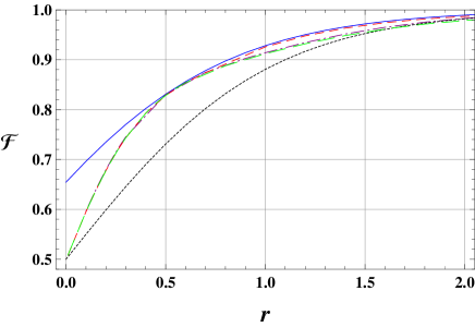
Figure 4: Comparison among the optimized fidelity of teleportation, Eq. (25), obtained using as entangled resources the class of optimized tunable states produced by our scheme in ideal conditions (red dashed line), the fidelity of teleportation obtained using as entangled resources the photon-subtracted squeezed state generated in ideal conditions (green large–dashed line), the ideal optimized fidelity obtained using as entangled resources the theoretical squeezed Bell states (cyan solid line), the fidelity obtained using as entangled resources the theoretical photon-subtracted squeezed states (purple dotted–dashed line), and the fidelity obtained using as entangled resources the theoretical Gaussian twin beams (black dotted line).

From this analysis, it emerges that in the ideal contest of state generation, the ideal optimized fidelity of teleportation is achieved, in the entire range of the considered values of $r$, by using as entangled resources the (optimized) theoretical squeezed Bell states Dellanno2007 . On the other hand, the optimal fidelity achievable using the class of states that can be generated by our experimental scheme in ideal conditions approximates remarkably well the ideal one associated to the theoretical squeezed Bell states for large enough values of the principal squeezing $r$.

It is also important to notice that while the fidelities associated to the theoretical states and to the photon-subtracted squeezed states generated in ideal conditions can be computed analytically as functions of $r$, the optimal fidelities associated to the entire class of states produced by our scheme in ideal conditions must be determined numerically point by point, so that the plots of these optimized fidelities, if seen in greater detail, would look as discrete, broken lines. In the plot range $0<$ $r\lesssim 2$ that represents the current levels of squeezing that are experimentally feasible Schnabel1 , we can then identify two distinct regimes:

a) $r\lesssim 0.5$ – the procedure of maximization Eq. (25) yields $s\simeq 0$, i.e. the best entangled resources generated by our scheme in ideal conditions coincide with states that approximate the photon-subtracted squeezed states generated in ideal conditions. On the other hand, the three curves corresponding, respectively, to the the optimized fidelity of teleportation, Eq. (25, obtained using as entangled resources the class of states produced by our scheme in ideal conditions, to the fidelity of teleportation obtained using as entangled resources the photon-subtracted squeezed state generated in ideal conditions, and to the fidelity of teleportation obtained using as entangled resources the theoretical photon-subtracted squeezed states, are superimposed and lie in between an upper limit given by the fidelity of teleportation obtained using as entangled resources the optimized theoretical squeezed Bell states and a lower limit given by the fidelity of teleportation obtained using as entangled resources the theoretical Gaussian twin beams.

b) $r>0.5$ – the optimized resources generated by our scheme outperform both the theoretical photon-subtracted squeezed states and those generated in ideal conditions, at the same time providing a performance very close to that of the optimized theoretical squeezed Bell states. In Fig. (5) we report their behaviors in the range $1\leq r\leq 2$. As an example, if we fix $r=1.6$, we obtain the value $0.974$ (at $s=0.056$) for the optimized fidelity of teleportation, Eq. (25, obtained using as entangled resources the photon-subtracted squeezed state generated in ideal conditions. At the same value of $r$, the teleportation fidelities obtained using as entangled resources the theoretical states are, respectively, $0.977$ for the optimized theoretical squeezed Bell state; $0.965$ for the theoretical photon-subtracted squeezed state; and $0.961$ for the theoretical Gaussian twin beam. Therefore, within the ideal conditions considered so far, the level of performance of the states generated by our scheme as entangled resources for quantum teleportation is remarkably close to that of the ideal theoretical states.

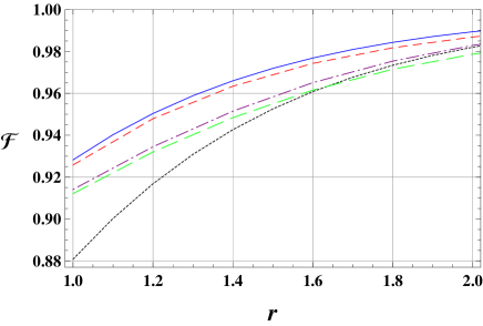
Figure 5: Zoom of Fig. (4) in the range $1\leq r\leq 2$ for: the optimized fidelity of teleportation obtained considering as entangled resources the optimized tunable states generated by our scheme in ideal conditions (red dashed line); the fidelity of teleportation obtained considering as entangled resources the photon-subtracted squeezed states generated in ideal conditions (green large–dashed line); the optimized fidelity of teleportation obtained considering as entangled resources the theoretical squeezed Bell states (cyan solid line); the fidelity of teleportation obtained considering as entangled resources the theoretical photon-subtracted squeezed states (purple dotted–dashed line); and the fidelity of teleportation obtained considering as entangled resources the theoretical Gaussian twin beams (black dotted line).

III.2 Realistic conditions

A realistic scenario of state generation within our scheme must include inefficient photon detection and a lossy environment for the input pair of two–mode squeezed states. In what follows we have considered the value $\eta=0.15$ for the detection efficiency (that is the value currently obtainable in real experiments). Moreover, we remark that the values of the squeezing amplitude $r$ which appear in the plots are referred to the theoretical principal squeezing, but the reduction to the effective squeezing $r^{{}^{\prime}}$ has been taken into account when displaying the final results.

In Fig. (6) we have plotted the optimized fidelity of teleportation, that depends on the squeezing amplitudes $r$ and $s$, assuming an overall transmissivity $T_{\ell}=0.85$, i. e. a level of loss equal to $0.15$, in Eq. (14). For consistency in the comparison between ideal and realistic conditions, in the figure we have plotted the optimized fidelity as a function of the ancillary squeezing $s$ ($\leq r$), assuming for the principal squeezing $r$ the same values as in Fig. (3). We can observe that:

a) The overall behavior of the fidelities does not change qualitatively, apart from a smoothing of the curves around their maximum.

b) As expected, the fidelities suffer a further deterioration due to the combined effect of losses and non–ideal single photon detection processes.

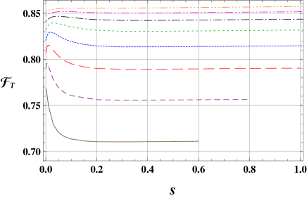
Figure 6: Fidelity of teleportation in a realistic lossy scenario (level of losses equal to $0.15$, i. e. $T_{\ell}=0.85$, and $\eta=0.15$), as a function of the ancillary squeezing $s$ ($\leq r$) for the same values of the principal squeezing $r$ of Fig. (3): (a) $r=0.6$ (brown solid line); (b) $r=0.8$ (purple dashed line); (c) $r=1$ (red large–dashed line); (d) $r=1.2$ (blue dotted line); (e) $r=1.4$ (green large–dotted line); (f) $r=1.6$ (black dotted–dashed line); (g) $r=1.8$ (magenta double dotted–dashed line); (h) $r=2$ (orange triple dotted–dashed line).

In this first plot the level of losses equals $0.15$. At present, this level is experimentally accessible by properly choosing optical components for the source of squeezing. On the other hand, very recently an outstanding source of squeezing with an overall loss of less than $0.08$ has been reported Schnabel2 . In view of this result, we have considered the behavior of the fidelities when the level of losses is varied.

Fixing the detection efficiency at $\eta=0.15$ and the principal squeezing parameter at $r=1.6$, in Fig. (7) we report the optimized fidelity of teleportation, Eq. (25, obtained considering as entangled resources the optimized tunable states generated by our scheme in realistic conditions, as a function of the loss parameter, denoted by $\ell$. In the same plot the optimal fidelity is compared with the fidelity of teleportation obtained considering as entangled resources the photon-subtracted squeezed states and the Gaussian twin beams generated in the same realistic conditions, i.e. with $\eta=0.15$ and $r=1.6$. As it can be seen, for losses up to $\ell=0.30$ the optimized tunable states generated by our scheme in realistic conditions always yield the largest fidelity of teleportation. It has to be noted that, at fixed principal squeezing $r$, the value of the ancillary squeezing $s$ corresponding to the maximum value of the optimized fidelity remains essentially constant. Indeed, in the case considered, this value varies in the interval $[0.048,0.050]$.

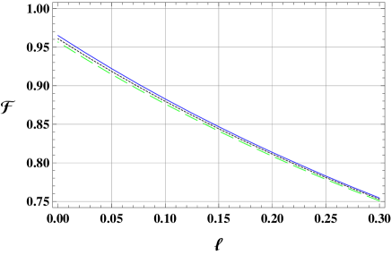
Figure 7: Optimized fidelity of teleportation (blue solid line) obtained considering as entangled resources the optimized tunable states generated by our scheme in realistic conditions, with $\eta=0.15$, plotted as a function of the loss parameter $\ell$, at fixed principal squeezing $r=1.6$. The optimized fidelity is compared with those obtained considering as entangled resources the photon-subtracted squeezed states ($s=0$, black dotted line)) and the Gaussian twin beams ($s=r$, green large–dashed line), generated in the same realistic conditions.

From Fig. (7) we see that in realistic conditions and for values of the principal squeezing $r$ varying in the interval $[1.2,1.6]$ the optimized tunable states yield fidelities of teleportation sizeably larger than those provided by photon-subtracted squeezed states and Gaussian twin beams. Furthermore, the behavior reported in Fig. (7) implies that foreseeable improvements in the control of losses could lead to levels of performance of the tunable non-Gaussian states comparable to those of the theoretical squeezed Bell states.

IV Discussion and outlook

In the present work we have introduced a scheme of state generation able to produce a class of tunable two-mode non-Gaussian states that approximate closely the class of theoretical squeezed Bell states introduced in Refs. Dellanno2007 ; Dellanno2010 . A thorough analysis yields that the states generated by our scheme in realistic conditions, when properly optimized by tuning two experimentally adjustable free parameters, provide, as entangled resources, the maximum fidelity of teleportation in the Braunstein-Kimble-Vaidman teleportation protocol of an unknown coherent state. Indeed, the optimized tunable non-Gaussian resources yield, in the most interesting range of the currently accessible experimental values of the principal squeezing amplitude $r$, a better performance both with respect to Gaussian twin beams and to photon-subtracted squeezed states, the latter being at present the best performing continuous-variable entangled resource that can be produced experimentally. This result holds true both in ideal and in realistic conditions. In particular, in ideal conditions of generation (no losses, perfect photon-resolving detection, perfect projections), for values of the principal squeezing $r>0.5$, the optimized tunable states show a level of performance very close to that of the optimized theoretical squeezed Bell states. In realistic conditions (presence of losses, only on/off measurements allowed), the optimized tunable states provide again, in a wide interval of values of the principal squeezing $r$, the best performance with respect to that yielded by Gaussian twin beams state and photon-subtracted squeezed states.

It is interesting to note that even a slight improvement, with respect to the current experimental situation, in reducing the level of losses and in increasing the detection efficiency would lead to a significant improvement in the performance of the optimal tunable states generated by our scheme in realistic conditions. As remarked in subsection III.B, a sizeable reduction of losses to very low levels seems at hand. Regarding the problem of improving the efficiency in photon-resolving procedures, detectors based on superconducting devices could lead to important progress in the near future Hadfield .

The theoretical study carried out in the present work proves that our scheme of state generation can produce a large class of two-mode non-Gaussian states that, when operated as entangled resources, can outperform both the currently available entangled two-mode Gaussian and de-Gaussified states. In forthcoming works, the experimental set up needed to realize our scheme of generation will be designed, analyzed, and discussed in all its technical details. To this end, we will consider two possible working regimes: continuous-wave regime and pulsed regime. We will also consider at length the problem of efficient detection in coincidence of two photons in two different modes, as this is one of the crucial requirements of our scheme, and we will show how the generated states can be reconstructed by performing suitable tomographic homodyne detections. Finally, further aspects of tunable non-Gaussian states will be investigated, in particular concerning protocols of entanglement swapping and distillation, as well as their properties with respect to Bell’s nonlocality and Einstein-Podolsky-Rosen steering.

V Acknowledgement

Daniela Buono, Fabio Dell’Anno, Silvio De Siena, and Fabrizio Illuminati acknowledge support from the EU STREP Project iQIT, Grant Agreement No. 270843.

VI Appendix A

Postselection: single-photon projector –

In the ideal scheme of state generation, Fig. (1), the post-selection strategy is based on ideal conditional measurements, i.e. simultaneous detections of single photons in mode $3$ and $4$. Such coincidence detections of single photons project the density matrix $\rho_{1234}$ into the tunable state $\rho_{\text{{T}}}^{\left(|1><1|\right)}$, which reads

$$\rho_{\text{{T}}}^{\left(|1><1|\right)}$$

$$\equiv\frac{\text{Tr}_{34}\left[\rho_{1234}\otimes\text{ }_{3}|1><1|_{3}\otimes\text{ }_{4}|1><1|_{4}\right]}{\mathcal{N}_{\text{{T}}}^{\left(|1><1|\right)}}$$

$$=\frac{1}{\mathcal{N}_{\text{{T}}}^{\left(|1><1|\right)}\pi^{4}}\int d^{2}\beta_{1}d^{2}\beta_{2}d^{2}\beta_{3}d^{2}\beta_{4}$$

$$\times\chi_{1234}\left(\beta_{1};\beta_{2};\beta_{3};\beta_{4}\right)D_{1}\left(-\beta_{1}\right)D_{2}\left(-\beta_{2}\right)$$

$$\times\text{Tr}_{\text{ }34}\left[D_{3}\left(-\beta_{3}\right)D_{4}\left(-\beta_{4}\right)_{3}|1><1|_{3\text{ }4}|1><1|_{4}\right]\text{ }$$

$$=\frac{\int d^{2}\beta_{1}d^{2}\beta_{2}\mathcal{M}^{\left(|1><1|\right)}\left(\beta_{1};\beta_{2}\right)D_{1}\left(-\beta_{1}\right)D_{2}\left(-\beta_{2}\right)}{\mathcal{N}_{\text{{T}}}^{\left(|1><1|\right)}\pi^{2}}\,.$$

In the above,

$$\mathcal{M}^{\left(|1><1|\right)}\left(\beta_{1};\beta_{2}\right)$$

$$\equiv\frac{1}{\pi^{2}}\int d^{2}\beta_{3}d^{2}\beta_{4}\chi_{1234}\left(\beta_{1};\beta_{2};\beta_{3};\beta_{4}\right)$$

$$\times\chi_{3}^{\left(|1>\right)}\left(\beta_{3}\right)\chi_{4}^{\left(|1>\right)}\left(\beta_{4}\right)\,.$$

Recalling that

$$<m|D\left(-\alpha\right)|n>=\left(\frac{n!}{m!}\right)^{1/2}\alpha^{m-n}e^{-|\alpha|^{2}/2}L_{n}^{m-n}\left(|\alpha|^{2}\right)\;,$$

and that $L_{1}^{0}\left(x\right)=L_{1}\left(x\right)=1-x$, one has

$$\chi_{k}^{\left(|1><1|\right)}\left(\beta_{k}\right) =\text{Tr}_{k}\left[\hat{D}_{l}\left(-\beta_{l}\right)_{3}|1><1|_{3}\right]$$

$$=\left(1-|\beta_{k}|^{2}\right)e^{-|\beta_{k}|^{2}/2}\text{ \ \ for }k=3,4\;,$$

which is the characteristic function of the single-photon projector, ${}_{k}|1><1|_{k}$, acting on the $k-$th mode. Moreover, the normalization constant $\mathcal{N}_{\text{{T}}}^{\left(|1><1|\right)}$ is given by

$$\mathcal{N}_{\text{{T}}}^{\left(\left|1\right\rangle\left\langle 1\right|\right)}\mathcal{=}\text{Tr}_{1234}\left[\rho_{1234}\otimes\text{ }_{3}\left|1\right\rangle\left\langle 1\right|_{3}\otimes\text{ }_{4}\left|1\right\rangle\left\langle 1\right|_{4}\right]\;.$$

In conclusion, we have

$$\chi_{\text{{T}}}^{\left(\left|1\right\rangle\left\langle 1\right|\right)}\left(\gamma_{1},\gamma_{2}\right)$$

$$=\frac{\text{Tr}_{12}\left[\rho_{12}D_{1}\left(\gamma_{1}\right)D_{2}\left(\gamma_{2}\right)\right]}{\mathcal{N}_{\text{{T}}}^{\left(\left|1\right\rangle\left\langle 1\right|\right)}}$$

$$=\frac{1}{\mathcal{N}_{\text{{T}}}^{\left(\left|1\right\rangle\left\langle 1\right|\right)}\pi^{2}}\int d^{2}\beta_{1}d^{2}\beta_{2}\mathcal{M}^{\left(|1><1|\right)}\left(\beta_{1};\beta_{2}\right)$$

$$\times\text{Tr}_{12}\left[D_{1}\left(\gamma_{1}\right)D_{1}\left(-\beta_{1}\right)D_{2}\left(\gamma_{2}\right)D_{2}\left(-\beta_{2}\right)\right]$$

$$=\frac{1}{\mathcal{N}_{\text{{T}}}^{\left(\left|1\right\rangle\left\langle 1\right|\right)}}\mathcal{M}^{\left(|1><1|\right)}\left(\gamma_{1};\gamma_{2}\right)\;.$$

Postselection: realistic on/off operator (POVM)–

In the realistic case, see Fig. (2), the post-selection strategy is based on realistic conditional measurements made by realistic on/off detectors. They are described by positive operator-valued measures (POVMs), Eq. (17). The detection $on-$POVM yields the state

$$\rho_{\text{{T}}}^{\left(on\right)} =\frac{\text{Tr}_{34}\left[\rho_{1234}\otimes\Pi_{3}^{(on)}\left(\eta_{3}\right)\otimes\Pi_{4}^{(on)}\left(\eta_{4}\right)\right]}{\mathcal{N}_{\text{{T}}}^{\left(on\right)}}$$

$$=\frac{1}{\mathcal{N}_{\text{{T}}}^{\left(on\right)}\pi^{4}}\int d^{2}\beta_{1}d^{2}\beta_{2}d^{2}\beta_{3}d^{2}\beta_{4}$$

$$\times\chi_{1234}\left(\beta_{1};\beta_{2};\beta_{3};\beta_{4}\right)D_{1}\left(-\beta_{1}\right)D_{2}\left(-\beta_{2}\right)$$

$$\times\text{Tr}_{34}\left[D_{3}\left(-\beta_{3}\right)D_{4}\left(-\beta_{4}\right)\Pi_{3}^{(on)}\left(\eta_{3}\right)\Pi_{4}^{(on)}\left(\eta_{4}\right)\right]$$

$$=\frac{1}{\mathcal{N}_{\text{{T}}}^{\left(on\right)}\pi^{4}}\int d^{2}\beta_{1}d^{2}\beta_{2}\mathcal{M}^{\left(on\right)}\left(\beta_{1};\beta_{2}\right)$$

$$\times D_{1}\left(-\beta_{1}\right)D_{2}\left(-\beta_{2}\right)\;,$$

where

$$\mathcal{M}^{\left(on\right)}\left(\beta_{1};\beta_{2}\right)$$

$$=\frac{1}{\mathcal{N}_{\text{{T}}}^{\left(on\right)}\pi^{2}}\int d^{2}\beta_{3}d^{2}\beta_{4}\chi_{1234}\left(\beta_{1};\beta_{2};\beta_{3};\beta_{4}\right)$$

$$\times\chi_{3}^{on}\left(\beta_{3}\right)\chi_{4}^{on}\left(\beta_{4}\right)\;.$$

Here

$$\chi_{k}^{on}\left(-\beta_{l}\right) \equiv\text{Tr}_{k}\left[D_{k}\left(-\beta_{k}\right)\Pi_{k}^{(on)}\right]$$

$$=\pi\delta^{(2)}\left(\beta_{k}\right)-\frac{1}{\eta_{k}}\exp\left\{-\frac{2-\eta_{k}}{2\eta_{k}}|\beta_{k}|^{2}\right\}$$

$$=\chi_{k}^{on}\left(\beta_{k}\right)$$

is the characteristic function of the POVM of the photo-detector of the modes $3$ and $4$, and the normalization reads

$$\mathcal{N}_{\text{{T}}}^{\left(on\right)}=\text{Tr}_{1234}\left[\rho_{1234}\otimes\Pi_{3}^{(on)}\left(\eta_{3}\right)\otimes\Pi_{4}^{(on)}\left(\eta_{4}\right)\right]\;.$$

The characteristic function corresponding to the density matrix $\rho_{\text{{T}}}^{\left(on\right)}$ is

$$\chi_{\text{{T}}}^{(on)}\left(\gamma_{1};\gamma_{2}\right) =\frac{1}{\mathcal{N}_{\text{{T}}}^{\left(on\right)}}\text{Tr}_{12}\left[\rho_{12}D_{1}\left(\gamma_{1}\right)D_{2}\left(\gamma_{2}\right)\right]$$

$$=\frac{1}{\mathcal{N}_{\text{{T}}}^{\left(on\right)}\pi^{2}}\int d^{2}\beta_{1}d^{2}\beta_{2}\mathcal{M}^{\left(on\right)}\left(\beta_{1};\beta_{2}\right)$$

$$\times\text{Tr}_{12}\left[D_{1}\left(-\beta_{1}\right)D_{2}\left(-\beta_{2}\right)D_{1}\left(\gamma_{1}\right)D_{2}\left(\gamma_{2}\right)\right]$$

$$=\frac{1}{\mathcal{N}_{\text{{T}}}^{\left(on\right)}\pi^{2}}\mathcal{M}^{\left(on\right)}\left(\gamma_{1};\gamma_{2}\right)\;.$$

In terms of the complex amplitudes $\beta_{1}$ and $\beta_{2}$, the characteristic function reads

$$\chi_{\text{{T}}}^{(on)}\left(\beta_{1};\beta_{2}\right)$$

$$=\frac{1}{\mathcal{N}_{\text{{T}}}^{\left(on\right)}\pi^{2}}\int d^{2}\beta_{3}d^{2}\beta_{4}\chi_{1234}\left(\beta_{1};\beta_{2};\beta_{3};\beta_{4}\right)$$

$$\times\chi_{3}^{on}\left(\beta_{3}\right)\chi_{4}^{on}\left(\beta_{4}\right)$$

$$=\frac{1}{\mathcal{N}_{\text{{T}}}^{\left(on\right)}}\left[\chi_{1234}\left(\beta_{1};\beta_{2};0;0\right)\right.$$

$$+\frac{1}{\pi}\int d^{2}\beta_{4}\chi_{1234}\left(\beta_{1};\beta_{2};0;\beta_{4}\right)\mathcal{G}_{4}\left(\beta_{4}\right)$$

$$+\frac{1}{\pi}\int d^{2}\beta_{3}\chi_{1234}\left(\beta_{1};\beta_{2};\beta_{3};0\right)\mathcal{G}_{3}\left(\beta_{3}\right)$$

$$\left.+\frac{1}{\pi^{2}}\int d^{2}\beta_{3}d^{2}\beta_{4}\chi_{1234}\left(\beta_{1};\beta_{2};\beta_{3};\beta_{4}\right)\mathcal{G}_{3}\left(\beta_{3}\right)\mathcal{G}_{4}\left(\beta_{4}\right)\right]\;,$$

where

$$\mathcal{G}_{k}\left(\beta_{k}\right) = -\frac{1}{\eta_{k}}\exp\left\{-\frac{2-\eta_{k}}{2\eta_{k}}|\beta_{k}|^{2}\right\}\;.$$

$$\left(k=3,4\right)\;.$$

Effective values of the squeezing amplitudes –

The values of the principal squeezing $r$ and of the ancillary squeezing $s$ are referred to the pure input parameters, before decoherence and losses affect the incoming beams and decrease the amplitudes to the real values $r^{\prime}$ and $s^{\prime}$. In the following we determine the relation holding between the squeezing parameters before and after the action of decoherence and losses. For this purpose, we express the two-mode squeezing operator $S_{ab}\left(-|\lambda|\right)$ in terms of single-mode squeezing operators $S_{c}\left(-|\lambda|\right),S_{d}\left(|\lambda|\right)$. These are obtained by introducing the transformed annihilation operators $c$ and $d$ defined by the linear superpositions

$$c = \frac{a+b}{\sqrt{2}}\;,$$

$$d = \frac{-a+b}{\sqrt{2}}\;.$$

Under this transformation, the two-mode squeezed state $S_{ab}\left(-|\lambda|\right)|\mathbf{0}>_{ab}$ goes into the two-mode squeezed state

$$S_{c}\left(-|\lambda|\right)S_{d}\left(|\lambda|\right)|\mathbf{0}>_{cd}\;,$$ (26)

where $S_{k}\left(\lambda\right)=\exp\left[-\frac{1}{2}\lambda k^{{\dagger}2}+\frac{1}{2}\lambda^{\ast}k^{2}\right],\left(k=c,d\right)$ denotes the single-mode squeezing operator. Introducing the fictitious beam splitters that simulate losses and decoherence, the original, decoherence-free state Eq. (26) becomes

$$|\psi>_{cd}=U_{c}\left(T_{\ell}\right)U_{d}\left(T_{\ell}\right)S_{c}\left(r\right)S_{d}\left(-r\right)|00>_{cd}\;,$$

where $U_{k}\left(T_{\ell}\right)$ is the beam splitter operator corresponding the $k$-th mode. Consequently, the characteristic function that describes the state $|\psi>_{cd}$ reads

$$\chi_{cd}\left(\beta_{c};\beta_{d}\right)=\text{Tr}\left[\rho_{cd}D_{c}\left(\alpha_{c}\right)D_{d}\left(\alpha_{d}\right)\right]\;,$$

where $\rho_{cd}=|\psi>_{cd\text{ }cd}<\psi|$. The variances of the modes $c$ and $d$ can be evaluated using the following property of the characteristic function:

$$\left(-\right)^{q}\frac{\partial^{p+q}}{\partial\alpha_{k}^{p}\partial\alpha_{l}^{\ast q}}\chi\left(\alpha\right)|_{\alpha,\alpha^{\ast}=0}=\text{Tr}\left[\rho_{cd}\left[\left(k^{{\dagger}}\right)^{p}l^{q}\right]_{\text{symmetric}}\right]\;,$$ (27)

with $k,l=c,d$. From this relation we can obtain the following variances:

$$\mathrm{Var}_{X_{c}}\left(T_{\ell}\right) = \mathrm{Var}_{Y_{d}}\left(T_{\ell}\right)=\frac{1-T_{\ell}\left(1-e^{2r}\right)}{2},$$ (28)

$$\mathrm{Var}_{X_{d}}\left(T_{\ell}\right) = \mathrm{Var}_{Y_{c}}\left(T_{\ell}\right)=\frac{1-T_{\ell}\left(1-e^{-2r}\right)}{2},$$ (29)

where

$$X_{k}=\frac{k+k^{{\dagger}}}{\sqrt{2}},\text{ \ \ \ \ \ \ }Y_{k}=i\frac{-k+k^{{\dagger}}}{\sqrt{2}}\text{\ ,}$$

are the quadrature operators corresponding to the $k$-th mode. Therefore, in realistic conditions, the lower limit for the variance $\mathrm{Var}_{X_{d}}\left(T_{\ell}\right)$ is $\left(1-T_{\ell}\right)/2$, corresponding to $r\rightarrow\infty$. When $T_{\ell}$ tends to $1$ (ideal case), the variances (28) and (29) tend, respectively, to the ideal values $e^{2r}/2$ and $e^{-2r}/2$, while the lower limit for the variance $\mathrm{Var}_{X_{d}}\left(T_{\ell}\right)$ vanishes.

If we denote by $r^{\prime}$ the effective, actually observed principal squeezing parameter, we have

$$\mathrm{Var}_{X_{d}}\left(T_{\ell}\right)=\frac{1}{2}e^{-2r^{\prime}}\;.$$

The inverse relation is

$$r^{\prime} = -\frac{1}{2}\ln\left[2\mathrm{Var}_{X_{d}}\left(T_{\ell}\right)\right]$$

$$= -\frac{1}{2}\ln\left[1-T_{\ell}\left(1-e^{-2r}\right)\right]\;.$$

Similar relations hold for the ancillary squeezing $s$. We may notice that if one lets the actually observed principal squeezing parameter $r^{\prime}$ go to zero, then the ideal squeezing parameter $r$ goes to zero as well $\forall$ $T_{\ell}$. There is no finite value of $r>0$ and $T_{\ell}$ such that the observed squeezing vanishes. This fact implies that decoherence can never attenuate the squeezing to vanishingly small values.

VII Appendix B

Formalism of the characteristic function –

In this appendix we describe in some detail the tunable states in terms of the characteristic function formalism.

The state $|\zeta>_{12}|\xi>_{34}$, Eq. (2), is the product of a pair of two independent two-mode squeezing states. Therefore, the characteristic function associated to the overall four-mode density matrix $\rho_{1234}$ corresponding to $|\zeta>_{12}|\xi>_{34\text{ }}$ reads as follows:

$$\chi^{\prime\prime}\left(\alpha_{12}^{\prime\prime};\alpha_{34}^{\prime\prime}\right)=\chi_{12}\left(\alpha_{12}^{\prime\prime}\right)\chi_{34}\left(\alpha_{34}^{\prime\prime}\right)\;,$$

where

$$\chi_{ij}\left(\alpha_{ij}^{{}^{\prime\prime}}\right)=\exp\left\{-\frac{1}{2}\left(\left|\varsigma_{i}\right|^{2}+\left|\varsigma_{j}\right|^{2}\right)\right\}\;,$$

and $\varsigma_{i,j}=\alpha_{i,j}^{\prime\prime}\cosh|\lambda|+\alpha_{j,i}^{\prime\prime\ast}e^{i\phi_{\lambda}}\sinh|\lambda|$, with $\lambda=\zeta$ if $i=1\wedge j=2$, and $\lambda=\xi$ if $i=3\wedge j=4$. In order to simulate the effect of decoherence, see Fig. (2), we have introduced four thermal beam splitters $TBS$ (one for each beam), with transmissivity $T_{th}\left(=1-R_{th}\right)$, in which each second port is impinged by the thermal state described by the following characteristic function:

$$\chi_{k}^{th}\left(\tau_{k}^{\prime}\right)=\exp\left\{-\frac{1}{2}\left(2\bar{n}_{k}^{th}+1\right)|\tau_{k}^{\prime}|^{2}\right\}\;,$$

where $\bar{n}_{th}$ is the average number of thermal quanta at equilibrium in the $k-$th mode:

$$\bar{n}_{k}^{th}=\left(e^{\hbar\omega/k_{B}T}-1\right)^{-1}\;.$$

The overall characteristic function before entering the thermal beam splitters, $\chi_{preTBS}$, describes the following eight-mode state:

$$\chi_{preTBS}\left(\alpha^{\prime\prime};\tau^{\prime}\right)=\chi^{\prime\prime}\left(\alpha^{\prime\prime}\right)\chi_{th}\left(\tau^{\prime}\right)\;,$$ (30)

where $\chi_{th}\left(\tau^{\prime}\right)=\prod\nolimits_{k=1}^{4}\chi_{k}^{th}\left(\tau_{k}^{\prime}\right)$. The beam splitters act on the state through a $SU(2)$ transformation that yields the following relation among the variables of the input and output modes:

$$\left\{\begin{array}[]{c}\alpha^{\prime}=\sqrt{T_{th}}\alpha^{\prime\prime}+\sqrt{R_{th}}\tau^{\prime}\;,\\ \tau=\sqrt{T_{th}}\tau^{\prime}-\sqrt{R_{th}}\alpha^{\prime\prime}\;.\end{array}\right.$$

Therefore the input modes are related to the output modes by the following linear transformation:

$$\left\{\begin{array}[]{c}\alpha^{\prime\prime}=\sqrt{T_{th}}\alpha^{\prime}-\sqrt{R_{th}}\tau\;,\\ \tau^{\prime}=\sqrt{T_{th}}\tau+\sqrt{R_{th}}\alpha^{\prime}\;.\end{array}\right.$$ (31)

Using the transformations Eq. (31), the characteristic function Eq. (30) describing the state after the passage through the four thermal beam splitters $BS_{th}$, depends on $\alpha^{\prime}$ and $\tau$, and reads:

$$\chi_{postTBS}\left(\alpha^{\prime};\tau\right) =\chi^{\prime\prime}\left(\sqrt{T_{th}}\alpha^{\prime}-\sqrt{R_{th}}\tau\right)$$

$$\times\chi_{th}\left(\sqrt{T_{th}}\tau+\sqrt{R_{th}}\alpha^{\prime}\right)\;.$$ (32)

Tracing out the thermal state by putting $\tau=0$, we are left with

$$\chi^{\prime}\left(\alpha^{\prime}\right) = \chi_{postTBS}\left(\alpha^{\prime};0\right)$$ (33)

$$= \chi^{\prime\prime}\left(\sqrt{T_{th}}\alpha^{\prime}\right)\chi_{th}\left(\sqrt{R_{th}}\alpha^{\prime}\right)\;.$$

The photon losses are introduced through four further beam splitters, $VBS$ ($V$ for “vacuum”), with transmissivity $T_{\ell}\left(=1-R_{\ell}\right)$, in which each second port is occupied by a vacuum mode:

$$\chi_{k}^{vac}\left(\upsilon_{k}^{\prime}\right)=\exp\left\{-\frac{1}{2}|\upsilon_{k}^{\prime}|^{2}\right\}\;,$$ (34)

with $\upsilon_{k}^{\prime}$ complex coherent amplitudes. Hence, the overall vacuum characteristic function is $\chi_{vac}\left(\upsilon^{\prime}\right)=\prod\nolimits_{k=1}^{4}\chi_{k}^{vac}\left(\upsilon_{k}^{\prime}\right)$. The overall characteristic function before the vacuum beam splitters, $\chi_{preVBS}$, reads

$$\chi_{preVBS}\left(\alpha^{\prime};\upsilon^{\prime}\right)=\chi^{\prime}\left(\alpha^{\prime}\right)\chi_{vac}\left(\upsilon^{\prime}\right)\;.$$ (35)

In this case, the $SU(2)$ transformation defines the relations

$$\left\{\begin{array}[]{c}\alpha=\sqrt{T_{\ell}}\alpha^{\prime}+\sqrt{R_{\ell}}\upsilon^{\prime}\;,\\ \upsilon=\sqrt{T_{\ell}}\upsilon^{\prime}-\sqrt{R_{\ell}}\alpha^{\prime}\;,\end{array}\right.$$ (38)

$$\left\{\begin{array}[]{c}\alpha^{\prime}=\sqrt{T_{\ell}}\alpha-\sqrt{R_{\ell}}\upsilon\,,\\ \upsilon^{\prime}=\sqrt{T_{\ell}}\upsilon+\sqrt{R_{\ell}}\alpha\,.\end{array}\right.$$ (41)

Thus, at the output of the beam splitters $VBS$, under the transformations Eq. (41), the characteristic function Eq. (35) has evolved into

$$\chi_{postVBS}\left(\alpha;\upsilon\right)$$

$$=\chi^{\prime}\left(\sqrt{T_{\ell}}\alpha-\sqrt{R_{\ell}}\upsilon\right)\chi_{vac}\left(\sqrt{T_{\ell}}\upsilon+\sqrt{R_{\ell}}\alpha\right)\;.$$

Tracing out the vacuum state ($\upsilon=0$), we are left with

$$\chi\left(\alpha\right) =\chi^{\prime}\left(\sqrt{T_{\ell}}\alpha\right)\chi_{vac}\left(\sqrt{R_{\ell}}\alpha\right)$$

$$=\chi^{\prime\prime}\left(\sqrt{T_{th}T_{\ell}}\alpha\right)\chi_{th}\left(\sqrt{R_{th}T_{\ell}}\alpha\right)$$

$$\times\chi_{vac}\left(\sqrt{R_{\ell}}\alpha\right)\;.$$

Considering the transformations produced by $BS_{I\text{ }}$ and $BS_{II\text{ }}$, for the complex variables $\alpha_{1};\alpha_{2};\alpha_{3};\alpha_{4}$, see Fig. (2), we have

$$\left\{\begin{array}[]{c}\alpha_{1}=\sqrt{T_{1}}\beta_{1}-\sqrt{R_{1}}\beta_{3}\;,\\ \alpha_{3}=\sqrt{T_{1}}\beta_{3}+\sqrt{R_{1}}\beta_{1}\;,\end{array}\right.$$

$$\left\{\begin{array}[]{c}\alpha_{2}=\sqrt{T_{2}}\beta_{2}-\sqrt{R_{2}}\beta_{4}\;,\\ \alpha_{4}=\sqrt{T_{2}}\beta_{4}+\sqrt{R_{2}}\beta_{2}\;,\end{array}\right.$$

so that the four-mode characteristic function $\chi\left(\alpha\right)$ is given by

$$\chi_{1234}\left(\beta_{1};\beta_{2};\beta_{3};\beta_{4}\right)$$ (44)

$$= \chi\left(\sqrt{T_{1}}\beta_{1}-\sqrt{R_{1}}\beta_{3};\sqrt{T_{2}}\beta_{2}-\sqrt{R_{2}}\beta_{4};\right.$$

$$\left.\sqrt{T_{1}}\beta_{3}+\sqrt{R_{1}}\beta_{1};\sqrt{T_{2}}\beta_{4}+\sqrt{R_{2}}\beta_{2}\right)\;.$$

Finally, the density matrix corresponding to the characteristic function $\chi_{1234}\left(\beta_{1};\beta_{2};\beta_{3};\beta_{4}\right)$ is

$$\rho_{1234}$$

$$=\frac{1}{\pi^{4}}\int d^{2}\beta_{1}d^{2}\beta_{2}d^{2}\beta_{3}d^{2}\beta_{4}\chi_{1234}\left(\beta_{1};\beta_{2};\beta_{3};\beta_{4}\right)$$

$$\times D_{1}\left(-\beta_{1}\right)D_{2}\left(-\beta_{2}\right)D_{3}\left(-\beta_{3}\right)D_{4}\left(-\beta_{4}\right)\;.$$

At optical frequencies, the characteristic field energy $\hbar\omega$ lies always in the range between $1.5$ and $2.5eV$, so that at room temperature $T\simeq 300K$, the average number of thermal photons $\bar{n}_{th}$ is of the order of $10^{-30}$. Therefore, the value of $\bar{n}_{th}$ is orders of magnitude smaller than the the mean number of photons associated to the various quantum sources and operators. For this reason, we have neglected throughout the thermal contribution to decoherence. In all cases, the ideal, decoherence-free state is recovered by putting $T_{\ell}=1$.

References

- (1) G. Adesso and F. Illuminati, J. Phys. A: Math. Theor. 40, 7821 (2007).
- (2) S. L. Braunstein and P. van Loock, Rev. Mod. Phys. 77, 513 (2005).
- (3) P. Kok, W. J. Munro, K. Nemoto, T. C. Ralph, J. P. Dowling, and G. J. Milburn, Rev. Mod. Phys. 79, 135 (2007).
- (4) J. Eisert and M. B. Plenio, Int. J. Quant. Inf. 1, 479 (2003).
- (5) F. Dell’Anno, S. De Siena, and F. Illuminati, Phys. Rep. 428, 53 (2006).
- (6) J. Eisert, S. Scheel, and M. B. Plenio, Phys. Rev. Lett. 89, 137903 (2002).
- (7) M. M. Wolf, G. Giedke, and J. I. Cirac, Phys. Rev. Lett. 96, 080502 (2006).
- (8) F. Dell’Anno, S. De Siena, L. Albano, and F. Illuminati, Phys. Rev. A 76, 022301 (2007).
- (9) F. Dell’Anno, S. De Siena, and F. Illuminati, Phys. Rev. A 81, 012333 (2010).
- (10) M. Ohliger, K. Kieling, and J. Eisert, Phys. Rev. A 82, 042336 (2010).
- (11) M. Ohliger and J. Eisert, Phys. Rev. A 85, 062318 (2012).
- (12) G. Adesso, F. Dell’Anno, S. De Siena, F. Illuminati, and L. A. M. Souza, Phys. Rev. A 79, 040305(R) (2009).
- (13) A. Monras and F. Illuminati, Phys. Rev. A 81, 062326 (2010).
- (14) A. Monras and F. Illuminati, Phys. Rev. A 83, 012315 (2011).
- (15) P. J. D. Crowley, A. Datta, M. Barbieri, and I. A. Walmsley, arXiv:1206.0043 (2012).
- (16) M. G. Genoni, M. G. A. Paris, G. Adesso, H. Nha, P. L. Knight, and M. S. Kim, Phys. Rev. A 87, 012107 (2013).
- (17) J. Hoelscher-Obermaier and P. van Loock, Phys. Rev. A 83, 012319 (2011).
- (18) K. Banaszek and K. Wodkiewicz, Acta Phys. Slov. 49, 491 (1999).
- (19) W. Son, J. Kofler, M. S. Kim, V. Vedral, and Ĉ. Brukner, Phys. Rev. Lett. 102, 110404 (2009).
- (20) A. Cabello and F. Sciarrino, Phys. Rev. X 2, 021010 (2012).
- (21) G. Cañas, J. F. Barra, E. S. Gómez, G. Lima, F. Sciarrino, and A. Cabello, Phys. Rev. A 87 012113 (2013).
- (22) A. Datta, L. Zhang, J. Nunn, N. K. Langford, A. Feito, M. B. Plenio, and I. A. Walmsley, Phys. Rev. Lett. 108, 060502 (2012).
- (23) E. T. Campbell, M. G. Genoni, and J. Eisert, Phys. Rev. A 87, 042330 (2013).
- (24) F. Dell’Anno, S. De Siena, and F. Illuminati, Phys. Rev. A 69, 033812 (2004).
- (25) F. Dell’Anno, S. De Siena, and F. Illuminati, Phys. Rev. A 69, 033813 (2004).
- (26) A. Zavatta, A. Viciani, and M. Bellini, Science 306, 660 (2004).
- (27) J. Wenger, R. Tualle-Brouri, and P. Grangier, Phys. Rev. Lett. 92, 153601 (2004).
- (28) K. Wakui, H. Takahashi, A. Furusawa, and M. Sasaki, Opt. Express 15, 3568 (2007).
- (29) A. Ourjoumtsev, A. Dantan, R. Tualle-Brouri, and P. Grangier, Phys. Rev. Lett. 98, 030502 (2007).
- (30) A. I. Lvovsky and S. A. Babichev, Phys. Rev. A 66, 011801 (2002).
- (31) V. D’Auria, C. de Lisio, A. Porzio, S. Solimeno, J. Anwar, and M. G. A. Paris, Phys. Rev. A 81, 033846 (2010).
- (32) V. D’Auria, A. Chiummo, M. De Laurentis, A. Porzio, and S. Solimeno, Opt. Express 13, 948 (2005).
- (33) L. Vaidman, Phys. Rev. A 49, 1473 (1994).
- (34) S. L. Braunstein and H. J. Kimble, Phys. Rev. Lett. 80, 869 (1998).
- (35) A. Furusawa, J. L. Sørensen, S. L. Braunstein, C. A. Fuchs, H. J. Kimble, and E. S. Polzik, Science 282, 706 (1998).
- (36) N. Lee, H. Benichi, Y. Takeno, S. Takeda, J. Webb, E. Huntington, and A. Furusawa, Science 332, 330 (2011).
- (37) T. Opatrny, G. Kurizki, and D.-G. Welsch, Phys. Rev. A 61, 032302 (2000).
- (38) P. T. Cochrane, T. C. Ralph, and G. J. Milburn, Phys. Rev. A 65, 062306 (2002).
- (39) S. Olivares, M. G. A. Paris, and R. Bonifacio, Phys. Rev. A 67, 032314 (2003).
- (40) G. Adesso and F. Illuminati, Phys. Rev. Lett. 95, 150503 (2005).
- (41) G. Li, S. Wu, and G. Huang, Phys. Lett. A 303, 11 (2002).
- (42) V. D’Auria, S. Fornaro, A. Porzio, S. Solimeno, S. Olivares, and M. G. A. Paris, Phys. Rev. Lett. 102, 020502 (2009).
- (43) D. Buono, G. Nocerino, V. D’Auria, A. Porzio, S. Olivares, and M. G. A. Paris, J. Opt. Soc. Am. B 27, A110 (2010).
- (44) V. D’Auria, S. Fornaro, A. Porzio, E. A. Sete and S. Solimeno, Appl. Phys. B 91, 309 (2008).
- (45) V. D’Auria, C. de Lisio, A. Porzio, S. Solimeno and M. G. A. Paris, J. Phys. B: At. Mol. Opt. 39, 1187 (2006).
- (46) D. Buono, G. Nocerino, A. Porzio and S. Solimeno, Phys. Rev. A86, 042308 (2012).
- (47) S.-L. Zhang and P. van Loock, Phys. Rev. A 84, 062309 (2011).
- (48) P. Marian and T. A. Marian, Phys. Rev. A 74, 042306 (2006).
- (49) T. Eberle, S. Steinlechner, J. Bauchrowitz, V. Händchen, H. Vahlbruch, M. Mehmet, H. Müller-Ebhardt, and R. Schnabel, Phys. Rev. Lett. 104, 251102 (2010).
- (50) S. Steinlechner, J. Bauchrowitz, T. Eberle, and R. Schnabel, Phys. Rev. A 87, 022104 (2013).
- (51) R. H. Hadfield, Nature Photonics 3, 696 (2009).