IMPACT OF TEMPERATURE DEPENDENT RESISTIVITY AND THERMAL CONDUCTION ON PLASMOID INSTABILITIES IN CURRENT SHEETS IN SOLAR CORONA

Abstract

In this paper we investigate, by means of two-dimensional magnetohydrodynamic simulations, the impact of temperature-dependent resistivity and thermal conduction on the development of plasmoid instabilities in reconnecting current sheets in the solar corona. We find that the plasma temperature in the current sheet region increases with time and it becomes greater than that in the inflow region. As secondary magnetic islands appear, the highest temperature is not always found at the reconnection $X$-points, but also inside the secondary islands. One of the effects of anisotropic thermal conduction is to decrease the temperature of the reconnecting $X-$points and transfer the heat into the $O-$points, the plasmoids, where it gets trapped. In the cases with temperature-dependent magnetic diffusivity, $\eta\sim T^{-3/2}$, the decrease in plasma temperature at the $X-$points leads to: (i) increase in the magnetic diffusivity until the characteristic time for magnetic diffusion becomes comparable to that of thermal conduction; (ii) increase in the reconnection rate; and, (iii) more efficient conversion of magnetic energy into thermal energy and kinetic energy of bulk motions. These results provide further explanation of the rapid release of magnetic energy into heat and kinetic energy seen during flares and coronal mass ejections. In this work, we demonstrate that the consideration of anisotropic thermal conduction and Spitzer-type, temperature-dependent magnetic diffusivity, as in the real solar corona, are crucially important for explaining the occurrence of fast reconnection during solar eruptions.

1 INTRODUCTION

Recent advanced solar observations suggest that plasmoids are ejected from reconnection sites in the solar corona both away and toward the Sun during Coronal Mass Ejections (CMEs), or solar eruptions Savage et al. (2010); Nishizuka et al. (2010); Milligan et al. (2010); Lin et al. (2005). Stemming from these observations, we can assume that the CME’s current sheet is not a single layer of enhanced current density, but it contains many fine structures within, including multiple reconnection X-points Lin et al. (2008). Since the majority of space plasma systems are collisionless, it is important to study the reconnection dynamics via the kinetic approach. The complexity of the underlying physics limits kinetic models and simulations of reconnection in these space environments to relatively small regions (size of ion-inertia length), which are currently under resolved with the existing observational facilities. The collisional theory, however, can still be used in numerous space plasma physics circumstances in order to calculate the reconnection rate, as well as the rate at which the magnetic energy is dissipated. Magnetohydrodynamic (MHD) reconnection solutions exist where the rate of reconnection is largely independent of the magnitude of the electric resistivity Priest & Forbes (2000). In physical circumstances high Lundquist numbers ($S\gtrsim 10^{4}$), existing numerical simulations have already demonstrated that a single reconnecting current sheet can break up into multiple interacting reconnection sites even on the MHD scale Biskamp (1986); Bhattacharjee et al. (2009); Huang et al. (2010); Shen et al. (2011); Barta et al. (2011); Mei et al. (2012). It was also found that, should the aspect ratio of the secondary current sheet exceed some critical value ($\gtrsim 60$), then higher orders of magnetic islands (or O-points) and thinner current sheets begin to develop Ni et al. (2010, 2012). As a result, the local value of current density at the X-points and the global reconnection rate can be increased significantly during the reconnection process involving plasmoid instabilities. This yields fast reconnection dynamics in the physical environment of the solar corona, as required to explain solar observations of flares and CMEs.

In the majority of existing MHD numerical studies of plasmoid instabilities, for simplicity, the magnetic diffusivity coefficient is assumed to be either uniform, or a function of position. For collisional space plasma on the MHD scale, it is well established, however, that the magnetic diffusivity varies with the plasma temperature approximately as: $\eta\sim T^{3/2}$ Spitzer (1962); Schmidt (1966). Since the plasma temperature in reconnecting current sheets is generally not uniform (varies with time and location), studying the reconnection process with a realistic, temperature-dependent magnetic diffusion is very important. Furthermore, the effects of thermal conduction on the reconnection dynamics in current sheets have also been ignored in the existing numerical 2-D (and 3-D) MHD models. Some previous studies, however, indicate that this term could be very important Takaaki & Kazunari (1997); Chen et al. (1999); Botha et al. (2011), should the temperature and its spatial gradient be high enough in the underlying physical environment, such as that of the solar corona.

On the choice of resistivity model in our simulations, note that there are numerous MHD models in the literature that adopt some (either ad-hoc, or physics-based) form of anomalous resistivity to obtain fast reconnection. For example, the MHD works of Roussev et al.Roussev et al. (2002) and Bárta et al.Barta et al. (2011) adopt physics-based models of anomalous resistivity to investigate the dynamics of fast reconnection in current sheets. In these studies, the anomalous resistivity is triggered by the drift velocity or electric currents exceeding some critical values. Some other studies Buchner & Elkina (2006); Nishikawa & Neubert (1996) have utilized particle-in-cell (PIC) codes to explore the nature of anomalous resistivity in reconnecting current sheets. What has been found so far is that the exact form(s) of anomalous resistivity used in the MHD models are not directly deducible from the kinetic theory and simulations of real physical systems, and therefore some simplifying assumptions are still required for the model of anomalous resistivity. For these reasons, we have refrained from using any model of anomalous resistivity in our high-$S$-number studies, and we demonstrate here that fast reconnection in the solar corona can be achieved even with the classical Spitzer-type resistivity.

In this paper, we investigate numerically the physical effects of temperature-dependent magnetic diffusivity and anisotropic thermal conduction on the evolution of plasmoid instabilities in reconnecting current sheets in the low solar corona. We analyze in great detail the spatial and temporal evolution of the current density, magnetic flux, reconnection rate, and temperature structure of reconnecting current sheet during the development of plasmoid instability process. The energy conversion process is also studied in great length and compared in the cases with and without thermal conduction. The organization of the paper is as follows. In Section 2, we present the resistive 2-D MHD equations utilized in this work, as well as the chosen initial and boundary conditions for the numerical experiments. Our scientific findings are presented and discussed in Section 3. Lastly, in Section 4, we summarize the results of our work and we outline future plans for research relevant to the subject.

2 FRAMEWORK OF NUMERICAL MODELS

The MHD equations describing the physical evolution of the low solar corona, including the effects of magnetic diffusion and anisotropic thermal conduction, are given by:

$$\partial_{t}\rho=-\nabla\cdot(\rho\textbf{v}),$$ (1)

$$\partial_{t}e=-\nabla\cdot[(e+p+\frac{1}{2}|\textbf{B}|^{2})\textbf{v}-(\textbf{v}\cdot\textbf{B})\textbf{B}]+\nabla\cdot[\eta\textbf{B}\times(\nabla\times\textbf{B})-\textbf{F}_{cond}],$$ (2)

$$\partial_{t}(\rho\textbf{v})=-\nabla\cdot[\rho\textbf{v}\textbf{v}+(p+\frac{1}{2}|\textbf{B}|^{2})I-\textbf{B}\textbf{B}],$$ (3)

$$\partial_{t}\textbf{B}=\nabla\times(\textbf{v}\times\textbf{B}-\eta\nabla\times\textbf{B}),$$ (4)

$$e=p/(\Gamma_{0}-1)+\rho\textbf{v}^{2}/2+\textbf{B}^{2}/2,$$ (5)

$$p=\rho T,$$ (6)

$$\textbf{F}_{cond}=-\kappa_{\parallel}(\nabla{T}\cdot\hat{\textbf{B}}){\hat{\textbf{B}}}-\kappa_{\perp}(\nabla{T}-(\nabla{T}\cdot\hat{\textbf{B}})\hat{\textbf{B}}).$$ (7)

The above equations are solved in 2-D space using the NIRVANA code (version 3.5) Ziegler (2008), and all the variables therein are dimensionless. The simulation domain ranges from $0$ to $1$ $(l_{x}=1)$ in the $x$-direction, and from $0$ to $4$ ($l_{y}=4$) in the $y$-direction. Here, $\rho$ is the plasma mass density, $e$ is the total energy density, v is the flow velocity, B is the magnetic field, $\hat{\textbf{B}}={\textbf{B}}/{|\textbf{B}|}$ is the unit vector in the direction of the magnetic field, $T$ is the temperature, $p$ is the plasma thermal pressure, and $\eta$ is the normalized magnetic diffusivity. Note here that $\eta$ can be chosen to be either uniform, or temperature-dependent in our models. The Lundquist number is defined by: $S=l_{y}v_{Ad}/\eta$, where $v_{Ad}$ is the initial normalized asymptotic Alfvén speed at the upstream boundary, which is set to 1.0 in all our models. The plasma is considered to be a fully ionized hydrogen gas, and the kinetic temperatures of ions and electrons are assumed to be equal. The ratio of specific heats, $\Gamma_{0}$, is set to $5/3$ (ideal gas). The parallel, $\kappa_{\parallel}$, and perpendicular, $\kappa_{\perp}$, thermal conductivity coefficients, in normalized form, are given by the Spitzer theory Spitzer (1962):

$$\kappa_{\parallel}=c_{1}\cdot\kappa_{SP},$$ (8)

$$\kappa_{\perp}=c_{2}\cdot 8.04\times 10^{-33}(\frac{\ln{\Lambda}}{m_{u}})^{2}\frac{{\rho}^{2}}{T^{3}B^{2}}\kappa_{SP}.$$ (9)

Here, $\kappa_{SP}=1.84\times 10^{-10}/({\ln{\Lambda}}T^{5/2})$ is the Spitzer’s thermal conductivity coefficient, $\ln{\Lambda}$ is the Coulomb logarithm set to $30$, $m_{u}=1.66057\times 10^{-27}kg$ is the atomic mass unit, $c_{1}=\mu_{0}T_{N}^{7/2}/(B_{N}^{2}L_{N}v_{A})$, and $c_{2}=\mu_{0}T_{N}^{1/2}\rho_{N}^{2}/(B_{N}^{4}L_{N}v_{A})$. Also, $T_{N}$, $B_{N}$, $L_{N}$ and $\rho_{N}$ are the normalization units for temperature, magnetic field, length, and mass density, respectively, of the system. The Alfvén speed is defined by $v_{AN}=B_{N}/\sqrt{\mu_{0}\rho_{N}}$, where $\mu_{0}=4\pi\times 10^{-7}$. Normally, the choice of normalization units is unimportant for resistive MHD, and the equations can be solved in normalized form for any values for $T_{N}$, $B_{N}$, $L_{N}$ and $\rho_{N}$. This is not true, however, for simulations that include the thermal conduction. From the expression of the heat conduction term, one can see that the physical values of the normalization units, along with the temperature gradient, determine the importance of this physical process. The importance of the cross-field thermal conduction coefficient, $\kappa_{\perp}$, is restricted to the strong magnetic field case. In the limit of vanishing field strength, the heat conduction becomes isotropic and $\kappa_{\perp}$ = $\kappa_{\parallel}$. In our model, this is accounted for by modifying $\kappa_{\perp}$ to be: $\kappa_{\perp}=min(\kappa_{\perp},\kappa_{\parallel})$. As a result, the cross-field heat conduction coefficient cannot be greater than the parallel one.

In our models, we consider a Harris current sheet as the initial condition for the magnetic field:

$$B_{y0}=b_{0}\tanh(\frac{x-0.5}{\lambda}),\quad B_{x0}=0.$$ (10)

Here $\lambda$ is the width of the current sheet set to $0.05$, and $b_{0}=1$. Note that the Harris current sheet should be thin enough to enable tearing instabilities to develop according to the criteria : $\frac{2}{\lambda}(\frac{1}{k\lambda}-k\lambda)>0$, where $k=2\pi/l_{y}$ is the wave number of the initial perturbations. The initial velocity is set to zero in all simulations. From Eq. 3, the plasma pressure must satisfy the initial equilibrium condition, which reads:

$$\nabla\cdot(p_{0}\textbf{I})=-\nabla\cdot[\frac{1}{2}|\textbf{B}_{0}|^{2}\textbf{I}-\textbf{B}_{0}\textbf{B}_{0}].$$ (11)

Since $\textbf{B}_{0}=B_{y0}\hat{\textbf{y}}$, where $\hat{\textbf{y}}$ is the unit vector in the $y$-direction, the initial equilibrium plasma pressure is calculated as:

$$p_{0}=-\frac{1}{2}B_{y0}^{2}+C_{0},$$ (12)

where $C_{0}$ is a constant. From Eq. 10, we know that $B_{y0}=1$ at the $x$-boundary. Since the kinetic gas pressure is related to the magnetic pressure by $\beta=\frac{p}{B^{2}/2}$, we obtain $C_{0}=\frac{\beta_{0}+1}{2}$, where $\beta_{0}$ is the initial plasma $\beta$ at the $x$-boundary. Thus:

$$p_{0}=\frac{1+\beta_{0}-B_{y0}^{2}}{2}.$$ (13)

The initial equilibrium value of the total energy is:

$$e_{0}=p_{0}/(\Gamma_{0}-1)+B_{y0}^{2}/2.$$ (14)

The initial temperature is assumed to be uniform in the entire simulation domain. From the ideal gas law $T=p/\rho$, the initial equilibrium mass density and temperature can be derived as:

$$\rho_{0}=p_{0}/T_{0}=\frac{1+\beta_{0}-B_{y0}^{2}}{\beta_{0}},\quad T_{0}=\frac{\beta_{0}}{2}.$$ (15)

In order to trigger plasmoid instabilities in the current sheet, we impose small initial perturbations for the magnetic field of the kind:

$$b_{x1}=-\epsilon\cdot 0.5\sin(\pi x/l_{x})\cos(2\pi y/l_{y}),$$ (16)

$$b_{y1}=\epsilon\cdot\cos(\pi x/l_{x})\sin(2\pi y/l_{y}).$$ (17)

In our simulations, we used a constant value of $\epsilon=0.05$. The introduced perturbation has a half-period in the $x$-direction and a full period in the $y$-direction. This type of perturbation yields the development of tearing-mode instabilities in the current sheet and it produces a large primary magnetic island. Eventually, a much thinner Sweet-Parker-type current sheet develops, and secondary magnetic islands appear if the Lundquist number is sufficiently large ($\gtrsim 10^{4}$). In all our simulations we impose periodic boundary conditions in the $y$-direction and Neumann boundary conditions in the the $x$-direction.

We have simulated five different physical scenarios (models M0-M4 hereafter), which are discussed in this paper. In models M0 and M1, the magnetic diffusivity is considered to be uniform everywhere. In Models M2-M4, the Lundquist number scales with the temperature as $S\sim T^{3/2}(x,y,t)$. We choose $S=\frac{4}{6}\times 10^{7}\times T^{3/2}$ in order to make the Lundquist number sufficiently high to yield the occurrence secondary plasmoid instabilities in the current sheet. The heat conducting term is included in models M1, M3 and M4, and the choice of the normalization units affects the significance of thermal conduction in the these cases. Table 1 summarizes the five different models. Note that the initial plasma $\beta_{0}$ is set to 0.2 in all the models. The normalization unit for temperature is set to $T_{N}=10^{7}$ K, and the initial temperature in the dimensional space is $T_{I}=\frac{\beta_{0}T_{N}}{2}=10^{6}$ K for cases M1, M3 and M4, which is similar to the temperature in the solar corona. In the real solar corona, the temperature could be higher than $10^{6}$ K, especially within current sheets. The magnetic field is of the order of $0.01$ T, and the mass density is around 1-2 orders of magnitude smaller than $9.576\times 10^{-10}\,kg/m^{3}$, so that the value of $c_{1}=\mu_{0}T_{N}^{7/2}/(B_{N}^{2}L_{N}v_{A})=\mu_{0}^{3/2}T_{N}^{7/2}\rho_{N}^{1/2}/(B_{N}^{3}L_{N})$ in the real solar corona could be close to, or even greater than the value of $c_{1}$ calculated for all the models. For the choice of normalization units in cases M1 and M3, we find that the magnitude of the cross-field thermal conduction coefficient is around $10^{8}$ times smaller than the parallel one at the boundaries $x=0$ and $x=1$. The thermal conduction, however, is nearly isotropic initially in the middle of the current sheet, because the magnetic field is weak there.

We perform the simulations on a base-level Cartesian grid of $80\times 320$. The highest refinement level in our simulations is 10, which corresponds to a grid resolution of $\delta x=1/81920$. In order to ensure that this resolution is sufficient, we have carried out convergence studies starting with twice lower resolution. In specific, we have tested the case M3 by setting the highest refinement level equal to 9, which corresponds to a grid resolution of $\delta_{x}=1/40960$. We find that the reconnection rate is very similar in both the high and the low resolution run. Hence, the grid resolution in our simulations is sufficiently high to suppress the effects of the numerical resistivity.

3 NUMERICAL RESULTS AND DISCUSSIONS

In this paper, the time-dependent reconnection rate is defined as $\gamma(t)=\partial(\psi_{X}(t)-\psi_{O}(t))/\partial t$, where $\psi_{X}$ and $\psi_{O}$ are the magnetic flux functions at the main reconnection $X$-point (where the separatrices separating the two open field line regions intersect) and the $O$-point. Here, the magnetic flux function is defined through the relations: $B_{x}=-\partial\psi/\partial y$, $B_{y}=\partial\psi/\partial x$. The $O$-point is always inside the primary island, and the corresponding $\psi_{O}$ is the minimum value of $\psi$ over the whole simulation domain. In the case when there are several $X$-points, the one which has the maximum value of $\psi$ dictates the reconnection rate. Calculated this way, the reconnection rate is the global one over the entire reconnecting current sheet.

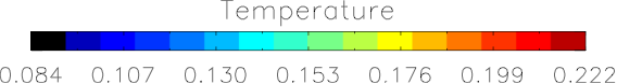
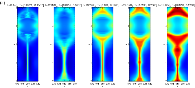
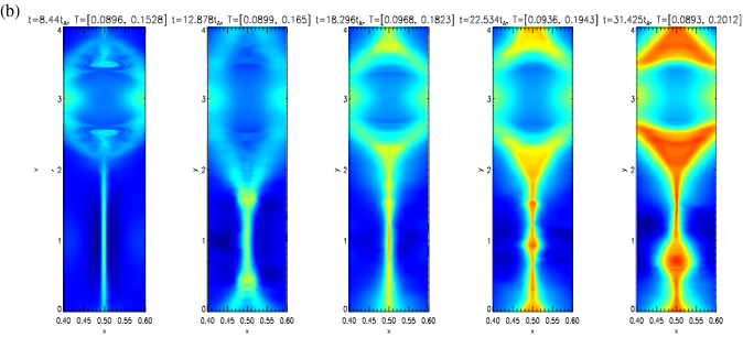
Figure 1: The spatial distribution of plasma temperature in the case M0 (a), case M2 (b), and case M3 (c) at different time instants.

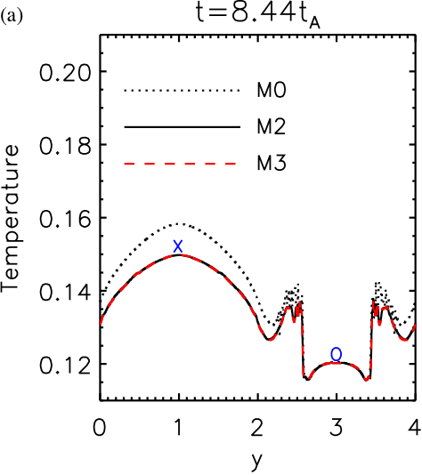
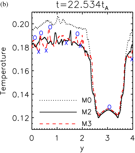
Figure 2: The distribution of the plasma temperature along the current sheet at $x=0.5$. The dotted black line is for case M0, the solid black line corresponds to the case M2, and the dashed red line is for the case M3. The blue ’O’ signs indicate the locations of the $O$-points in case M3, whereas the blue ’X’ signs mark the position of the reconnection $X$-points. Panel (a) represents a time instant before the secondary islands appear, and panel (b) is for a time instant when the secondary islands are present.

While analyzing the data, we find the following key observations. First, the temperature increases with time at the center of the current sheet, especially at the reconnection $X$-point in the beginning. Since the plasma is ejected away from the $X$-point during the development of plasmoid instability process, an increasing amount of hot plasma gets trapped inside the magnetic islands. The location of maximum temperature is sometimes found not to be at the reconnection $X$-point, but inside the secondary islands. The temperature in the current sheet region, however, is always higher than in the inflow region. Once can see this characteristic evolution of the temperature in Fig. 1 and Fig. 2.

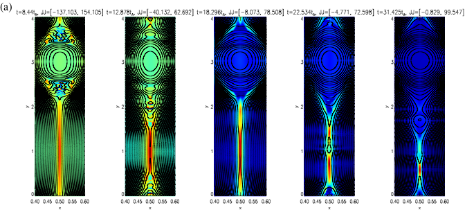
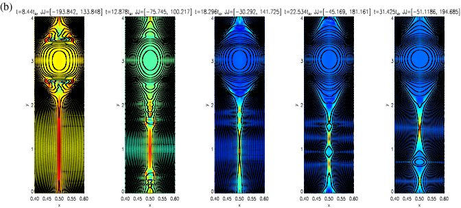
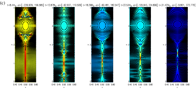
Figure 3: The spatial distributions of the current density and the magnetic flux in the case M0 (a), the case M2 (b), and the case M3 (c) at different time instants.

For a temperature-dependent magnetic diffusivity ($\eta\sim T^{-3/2}$), $\eta$ decreases with increasing temperature. Fig. 3(a) and Fig. 3(b) illustrate the distributions of the current density and the magnetic flux at different time instants for the case of uniform magnetic diffusivity (M0), and the case of temperature-dependent magnetic diffusivity (M2), respectively. Since the initial temperature, $T_{0}$, is set to 0.1 in all the cases we have simulated here, the initial value of magnetic diffusivity is the same in all cases. As the plasmoid instability develops with time in the case M2, the magnetic diffusivity inside the current sheet decreases with increasing temperature. This makes the initial thick Harris sheet evolve into a thinner Sweet-Parker current sheet, when compared with the M0 case (with uniform magnetic diffusivity). There also appear more secondary islands and thinner secondary current sheets in the case M2 than in the case M0. The maximum current density at the $X$-point in the case M2 can increase to higher values during the secondary instabilities. At the same time, however, the reconnection rate and the maximum temperature in the simulation domain are somewhat smaller than in the case M0. These key observations can be seen clearly in Fig. 2, Fig. 3(a), Fig. 3(b), Fig. 4(a) and Fig. 4(b). Fig. 2 also shows that the temperature distribution along the current sheet is relatively smoother for the case of uniform magnetic diffusivity (M0). According to the normalization units chosen for cases M1 and M3, the ion-inertia length is calculated to be around $100$ m in these models. The narrowest width of the secondary current sheets can reach around 0.001 in our simulations, which corresponds to $0.001L_{C}=10^{4}$ m in the real space. This is much greater than the ion-inertia length, meaning that our simulations are in the collisional regime. Therefore, the adopted form of temperature-dependent magnetic diffusivity is well justified in our models.

In the following we discuss the physical effects of thermal conduction on the development of the plasmoid instabilities. The numerical results for the reconnection rate, the current density distribution, the temperature distribution, and the energy conversion are presented and compared for the cases with and without thermal conduction.

In the case with uniform magnetic diffusivity (M1), the heat conduction (see Table 1 for characteristic parameters) does not affect significantly the evolution of the plasmoid instability. The reconnection rate, the distribution of the current density, and the magnetic field structure at each time step for the case M1 are very similar to those for the case M0. The cases M2, M3, and M4 have the same form of magnetic diffusivity, which evolves with temperature as $\eta\sim T^{-3/2}$. The thermal conduction term, however, is switched on only in cases M3 and M4 (and turned off for M2). Also, the normalization units are the same in the cases M1 and M3, unlike the case M4 where the normalization units for magnetic field strength and mass density are chosen smaller. This makes the value of $c_{1}$ greater in the case M4 than in the cases M1 and M3, which is why the thermal conduction effects more pronounced in the former. We find that the spatial and temporal evolution of the current density and the magnetic flux to be almost identical for the cases M2-M4 prior to the occurrence of secondary magnetic islands. As the plasma temperature and its gradient increase in the current sheet during secondary instability processes, the heat conduction effects become more pronounced in the case M4 than in the other cases. Note that the time-step becomes very small after $t=22t_{A}$ in the case M4, which is why the simulation was terminated at this time.

As far as the time-dependent current-sheet structure and reconnection rate are concerned, one can see In Fig. 3(b) and Fig. 3(c) that the secondary current sheets are thinner in the case M3 than in the case M2 at the same time instant. We also find that in the former case the maximum current density at the reconnection $X$-point increases up to a value is twice greater than in the latter case. Fig. 4(a) reveals that the reconnection rate is also almost twice greater in the case M3 than in the case M2 during the later stages of the secondary instability process. In the case of M4, the reconnection rate can increase to an even higher value compared to the cases M2-M3. As seen in Fig. 2(b), when there are secondary plasmoids present in the current sheet, the temperature distribution along the current sheet is not smooth anymore, and there are several temperature peaks inside the secondary plasmoids. This makes the temperature gradients along the current sheet become large enough to render the heat conduction important. This leads to a further increase in the reconnection rate, as seen in the case of M4.

In order to demonstrate the significance of thermal conduction, we calculate the characteristic time-scale of heat conduction , $t_{TH}\sim E_{th}/(\kappa_{\parallel}\partial^{2}T/\partial x^{2})$ along the current sheet in the case M3 at $t=22.534t_{A}$. Here, $E_{th}$ is the thermal energy density, $\kappa_{\parallel}$ is the field-aligned thermal conduction coefficient, and $\partial^{2}T/\partial x^{2}$ is the second derivative of plasma temperature. We find that $t_{TH}$ is significantly shorter ($\sim 0.1t_{A}$) than the Alfvén crossing time at the reconnection $X$-point locations, as well as the $O$-point locations than elsewhere in the current sheet. Note, however, that at the locations of the $O$-points the temperature gradient is across the magnetic field, meaning that it is $\kappa_{\perp}$ that determines the $t_{TH}$ in the above expression. Since $\kappa_{\perp}\ll\kappa_{\parallel}$, the thermal conduction will be inefficient in getting heat out of the plasmoids, hence their plasma temperature will grow in time. When comparing the cases with and without thermal conduction, we find that the significance of this process is in lowering the plasma temperature (and heat content) at the locations of the $X-$points, while increasing the temperature (and heat content) of the adjacent plasmoids (or the $O-$point locations). The drop in temperature at the locations of the $X-$points means higher value of the magnetic diffusion coefficient ($\sim T^{-3/2}$) there, hence: (i) more efficient conversion of magnetic energy into heat and kinetic energy; and, (ii) enhanced reconnection rate, as in the case M4. We find that in the temperature-dependent magnetic diffusivity cases, the plasma temperature increases from 0.1 (initially) to around 0.25 inside the current sheet region, which leads to a decrease in the magnetic diffusivity by a factor of 4 from its initial value of $1.89\times 10^{-5}$ down to $4.8\times 10^{-6}$. As the temperature rises at the locations of the $X-$points, however, the effects of thermal conduction increase, leading to a drop in plasma temperature on a characteristic time-scale of $t_{TH}$, which is shorter than the characteristic time of magnetic diffusion, $t_{MD}\sim{d_{X}}^{2}/\eta$ (where $d_{X}$ is the characteristic size of the diffusion region). As a consequence, the drop in temperature at the $X-$points results in an enhanced $\eta$ therein which, in turn, leads to a decrease in $t_{MD}$. This negative-feedback-loop proceeds until $t_{MD}$ becomes comparable with $t_{TH}$, which is achieved at enhanced values of $\eta$. This ultimately leads to an enhanced reconnection rate at the $X-$points due to the presence of thermal conduction. This is also the reason why the thermal conduction is more effective in the case M3 with temperature-dependent resistivity than in the case M1 with uniform resistivity.

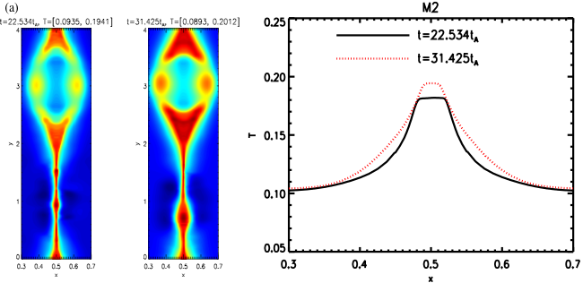
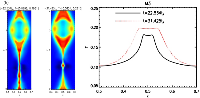
Figure 5: The spatial distribution of the plasma temperature at time instants $t=22.534t_{A}$ and $t=31.425t_{A}$. These are shown in the region from $x=0.3$ to $x=0.7$ for the case M2 (a) and the case M3 (b). The third plot to the right in both cases illustrate the plasma temperature distribution at $y=4$ along the $x$-direction in the primary magnetic island.

The time-dependent temperature distributions in the cases M2 and M3 are found to be different during the later stages of the secondary instability process. One can see in Fig. 1(b) , Fig. 1(c), Fig. 2(a), and Fig. 2(b) that the plasma temperature distributions inside the current sheet for these two cases are almost identical prior to the secondary islands appearance. From the discussion above, the appearance of secondary islands enhances the effects of thermal conduction, as in the case M3, which makes the temperature distribution along the current sheet different than that in the case without thermal conduction (case M2). The first and the second plots from left to right in Fig. 5(a) and Fig. 5(b) reveal the temperature distribution for the case M2 and the case M3, respectively, $t=22.534t_{A}$ and $t=31.425t_{A}$. In these figures, one can see that the hot plasma trapped in the primary plasmoid is more spread out in the $x$-direction (at the same $y$ location) in the case M3 than in the case M2 at $t=31.425t_{A}$. The third plots to the right in Fig. 5(a) and Fig. 5(b) show the temperature distribution in the $x$-direction at $y=4$ for the case M2 and the case M3, respectively. During the time period from $t=22.534t_{A}$ to $t=31.425t_{A}$, the highest temperature region spreads out in the $x$-direction to a larger extent in the case M3 than in the case M2. This is because a thermal, front-like structure propagates away from the center-line of the current sheet along the x-axis in the case M3. The enhanced heat content (and plasma pressure) inside the plasmoid (more enhanced in the case M3 than in the case M2 due to the heat conduction) causes a new pressure balance to be reached at a greater width of the plasmoid in the $x$-direction.

Note here that we have utilized anisotropic thermal conduction in the models discussed here, and the cross-field conduction coefficient ($\kappa_{\perp}$) is much smaller than the field-aligned conduction coefficient ($\kappa_{\parallel}$) inside the entire current sheet. We find that $\kappa_{\perp}$ is comparable in value to $\kappa_{\parallel}$ (and hence isotropic) only inside a narrow region ranging from $x=0.4998$ to $x=0.5002$ where the magnetic field is negligible. The width of this region is even more narrower that the width of the secondary current sheets that are present in our models. Therefore, the heat conduction is anisotropic almost everywhere in the simulation domain, and it changes the distribution of plasma temperature only along the magnetic field. This is the reason why the heat can not be conducted away in the direction perpendicular to the current sheet.

In order to quantify the differences between the cases with (M3) and without (M2) thermal conduction during the development of plasmoid instabilities, we calculate the various energy contents (and fluxes) inside the region given by: $0.4\leq x\leq 0.6$ and $0\leq y\leq 4$. Due to the non-vanishing energy fluxes through the boundaries at $x_{b}=0.4$ and $x_{e}=0.6$, the total magnetic, thermal, and kinetic energy inside this region changes in time during the plasmoid instability process. The magnetic, thermal, and kinetic energy flowing into this region through the boundaries at $x_{b}=0.4$ and $x_{e}=0.6$ from the beginning of the simulation ($t=0$) to time $t$ is denoted as $E_{MF}(t)$, $E_{TF}(t)$, and $E_{KF}(t)$, respectively. (Note that these quantities may have negative signs if energy flows out of the region.) The magnetic, thermal, and kinetic energy confined to this region at time $t$ is denoted as $E_{ML}(t)$, $E_{TL}(t)$, and $E_{KL}(t)$, respectively. The initial magnetic, thermal, and kinetic energy at $t=0$ is denoted as $E_{MI}$, $E_{TI}$, and $E_{KI}$, respectively. In these notations, the dissipated magnetic energy in the region defined by $0.4\leq x\leq 0.6$ and $0\leq y\leq 4$, is given by: $E_{MD}(t)=E_{MI}+E_{MF}(t)-E_{ML}(t)$. In the same region, the generated thermal energy is $E_{TG}(t)=E_{TL}(t)-E_{TF}(t)-E_{TI}$, and the generated kinetic energy is $E_{KG}(t)=E_{KL}{t}-E_{KF}(t)-E_{KI}$. The explicit expressions for these quantities are:

$$E_{MF}(t)=\int_{0}^{t}\!\!\!\int_{0}^{4}[v_{x}(0.4,y,t)B_{y}(0.4,y,t)-v_{y}(0.4,y,t)B_{x}(0.4,y,t)-{}$$

$$\eta(0.4,y,t)(\partial_{x}B_{y}(0.4,y,t)|_{x=0.4}-\partial_{y}B_{x}(0.4,y,t))]B_{y}(0.4,y,t)\,\mathrm{d}y\,\mathrm{d}t-{}$$

$$\int_{0}^{t}\!\!\!\int_{0}^{4}[v_{x}(0.6,y,t)B_{y}(0.6,y,t)-v_{y}(0.6,y,t)B_{x}(0.6,y,t)-{}$$

$$\eta(0.6,y,t)(\partial_{x}B_{y}(0.6,y,t)|_{x=0.6}-\partial_{y}B_{x}(0.6,y,t))]B_{y}(0.6,y,t)\,\mathrm{d}y\,\mathrm{d}t,$$ (18)

$$E_{TF}(t)=\int_{0}^{t}\!\!\!\int_{0}^{4}(\frac{\Gamma_{0}p(0.4,y,t)}{\Gamma_{0}-1}v_{x}(0.4,y,t)+F_{cond}|_{x=0.4})\,\mathrm{d}y\,\mathrm{d}t-{}$$

$$\int_{0}^{t}\!\!\!\int_{0}^{4}(\frac{\Gamma_{0}p(0.6,y,t)}{\Gamma_{0}-1}v_{x}(0.6,y,t)+F_{cond}|_{x=0.6})\,\mathrm{d}y\,\mathrm{d}t$$ (19)

$$E_{KF}(t)=\int_{0}^{t}\!\!\!\int_{0}^{4}\rho(0.4,y,t)\frac{(v_{x}^{2}(0.4,y,t)+v_{y}^{2}(0.4,y,t))}{2}v_{x}(0.4,y,t)\,\mathrm{d}y\,\mathrm{d}t-{}$$

$$\int_{0}^{t}\!\!\!\int_{0}^{4}\rho(0.6,y,t)\frac{(v_{x}^{2}(0.6,y,t)+v_{y}^{2}(0.6,y,t))}{2}v_{x}(0.6,y,t)\,\mathrm{d}y\,\mathrm{d}t,$$ (20)

$$E_{ML}(t)=\int_{0}^{4}\!\!\!\int_{0.4}^{0.6}\frac{B_{x}^{2}(x,y,t)+B_{y}^{2}(x,y,t)}{2}\,\mathrm{d}x\,\mathrm{d}y,$$ (21)

$$E_{TL}(t)=\int_{0}^{4}\!\!\!\int_{0.4}^{0.6}\frac{p(x,y,t)}{\Gamma_{0}-1}\,\mathrm{d}x\,\mathrm{d}y,$$ (22)

$$E_{KL}(t)=\int_{0}^{4}\!\!\!\int_{0.4}^{0.6}\frac{\rho(x,y,t)(v_{x}^{2}(x,y,t)+v_{y}^{2}(x,y,t))}{2}\,\mathrm{d}x\,\mathrm{d}y$$ (23)

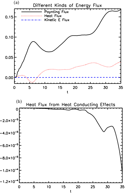
Figure 6: (a) The time-dependent evolution of the different types of energy fluxes flowing into the dissipation region through the boundaries at $x=0.4$ and $x=0.6$ for the case M3. (b) Time-dependent evolution of the heat flux conducted into the dissipation region for the case M3.

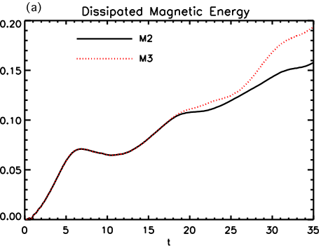
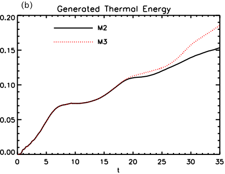
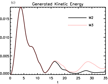
Figure 7: The time-dependent evolution of the dissipated magnetic energy, the thermal energy, and the kinetic energy in the dissipation domain defined in the main text.

The thermal energy flowing into this region consists of two parts. The first part comes from the inward enthalpy flux through the boundaries at $x=0.4$ and $x=0.6$. The second part comes from the thermal conduction effects in the $x$-direction. The integral calculations of the different types of energy fluxes have been performed in IDL. We have doubled the spatial and temporal resolutions to check the results and make sure that they have converged. In Fig. 6(a) we show the time-dependent evolution of the different kinds of energy fluxes through the $x$-boundaries. One can see that a substantial amount of magnetic energy flows into the region during the period from $t=0$ to $t=35t_{A}$ during the development of the plasmoid instability process. On the contrary, we find that a relatively smaller amount of thermal and kinetic energy have flown into the region for the same time period. Fig. 6(b) reveals that the thermal energy conducted out of this region in the $x$-direction due to the thermal conduction can be ignored in the case M3. The thermal energy flux in the $x$-direction is basically brought in by the enthalpy flux from the inflow region. Fig.7(a), Fig.7(b), and Fig.7(c) visualize the time-evolution of the dissipated magnetic energy, the generated thermal energy, and the generated kinetic energy, respectively, for the cases M2 and M3. In these figures, one can see that the dissipated magnetic energy is not always increasing with time, but it decreases slightly from $t=6.5t_{A}$ to $t=11t_{A}$. That is because the advection of magnetic flux from the inflow region is more dominant that the dissipation of magnetic flux during this time period, which leads to the slight increase in magnetic energy during this time period. We find that the generated thermal energy increases monotonically with time during the secondary instability process. The generated kinetic energy is much less than the generated thermal energy during the entire instability process, and we find that the former is not always increasing with time. In the cases M2 and M3 there are several peaks in the kinetic energy from $t=0$ to $t=35t_{A}$, with the maximum peak reached at around $t=3.8t_{A}$ (before the secondary instabilities occur). Therefore, there is more kinetic energy generated during the primary tearing instability process than during the secondary instability process. In other words, some portion of the generated kinetic energy has been converted to other forms of energy (thermal) after $t=3.8t_{A}$. The magnetic energy is found to be dissipated faster in the case M3 than in the case M2 during the later stages of the secondary instability process. There is also more thermal energy generated in the case M3 than in the case M2 during the advanced stages of secondary instabilities. The secondary peaks seen in the case M3 are more pronounced (higher amplitude) than in the case M2. Although approximately 99% of the magnetic energy has been eventually transformed into thermal energy, we find that the energy conversion process during the development of the plasmoid instabilities is rather complex. Another key result is that there has been more magnetic energy transformed into thermal and kinetic energy in the case M3 than in the case M2, because the reconnection rate is higher in the former (see discussion above). This demonstrates once again that the thermal conduction acts to accelerates the reconnection rate during the plasmoid instabilities process. Should the simulation in the case M4 be run further to $t=35t_{A}$, then one can also calculate the energy transformation processes for this case and compare them to those in the cases M2 and M3. Since the thermal conduction effects are stronger in the case M4 than in the case M3, during the same time period, there should be more magnetic energy transformed into thermal and kinetic energy in the case M4 than in the case M3.

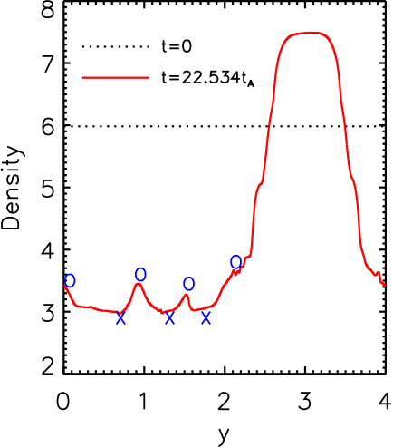
Figure 8: The distribution of the plasma density along the current sheet at $x=0.5$. The dotted black line corresponds to $t=0$, and the solid red line is for $t=22.534t_{A}$. The blue ’O’ signs indicate the locations of the $O$-points of the secondary plasmoids, whereas the blue ’X’ signs mark the position of the reconnection $X$-points.

Note here that the purpose of this paper was to investigate the effects of thermal conduction alone on the reconnection dynamics, as well as on the dynamics of the secondary instability processes. However, should the radiative cooling be included along with some ad-hoc volumetric heating to achieve initial energy balance in our model, here is what we would observe over the course of the simulation. First, the temperature variations ($1.0-2.5\times 10^{6}K$) within the current sheet in our simulation are in the regime where the radiative loss function is weakly dependent (and rather uniform) on the electron temperature. Therefore, the differences in radiative cooling will be entirely due to the electron density (squared) fluctuations. As can be seen in Fig. 8, the electron density along the mid-line of the current sheet (at $x=0.5$) has dropped almost by a factor of 2 everywhere at $t=22.5t_{A}$, except for the primary magnetic island where it has increased by $20-30\%$. Therefore, in the former region, the radiative cooling rate will drop by a factor of 4, whereas in the latter region it will increase by $1.45-1.7$ times. In other words, the primary magnetic island will experience some enhanced radiative cooling, which will directly compete with the time-dependent heat increase inside the island due to the thermal conduction. In the region where the electron density drops almost twice compared to the initial value, the radiative cooling rate will drop by a factor of 4, but at the same time, the background volumetric heating (for which there is no sensible model of how to evolve in time) will provide excessive heating in this region. Hence, the temperature of the secondary current sheets, including the secondary plasmoids, will increase with time. Note that, although the electron density along the mid-line of the current sheet drops with time, it is still around $16\%$ higher at the $O$-points inside the secondary islands than the $X$-points of the secondary current sheets, as seen in Fig. 8. Therefore, the radiation cooling will be around $35\%$ stronger at the $O$-points inside the secondary islands than the $X$-points of the secondary current sheets. Hence, due to the excessive volumetric heating in the latter than in the former, the maximum temperature would be observed at the reconnection $X$-points. In summary, the thermal conduction and the radiative cooling will act in a competing fashion on the dynamics of the reconnecting current sheet. It should be noted here, however, that the biggest uncertainty in a model that includes the radiative cooling is in the assumed form of the volumetric heating rate. This heating can be constructed such that there is an energy balance initially in the model, but then we cannot assume any physically meaningful temporal evolution of this heating function in time.

Here, we would like to discuss briefly the relationship between the Lundquist number, $S$, in our simulations and the obtained rate of reconnection. The highest $S$ in our simulations is found to around $10^{6}$ as the temperature is increased to $2.5\times 10^{6}K$. In order to ensure that the numerical resistivity is much smaller than the physical (Spitzer-type) resistivity adopted in our models, high numerical resolution is needed when the Lundquist number is high. As is known, the Lundquist number in the real solar corona is around $10^{12}$, which is beyond our computational capabilities at present. Some recent simulation studies Bhattacharjee et al. (2009); Huang et al. (2010); Ni et al. (2010, 2012) have indicated, however, that the reconnection rate weakly depends on the Lundquist number as secondary instabilities appear and $S$ exceeds a critical value. Therefore, in some sense, $S=10^{6}$ can represent the physical conditions seen in reconnecting current sheets in the solar corona. These previous studies also demonstrate that the reconnection rate can increase up to a high value of $\gamma\sim 0.01$ during the secondary instability processes. There are also independent theoretical calculationsGuo et al. (2012), which have shown that the hyper-diffusivity could be an important physical process yielding fast reconnection during the secondary instability processes. In order to make the reconnection environment more similar to the real solar corona, the plasma $\beta$ at the inflow boundaries in our models is chosen to be smaller than $1.0$, and the mass density inside the current sheet in the center is around $6$ times higher than the inflow regions, so the plasmas in our simulations are compressible. One of our recent worksNi et al. (2012) has demonstrated that the plasma $\beta$ at the inflow boundary can make the plasmoid instability process and the reconnection rate very different, the reconnection rate for the higher $\beta$ case is greater than the lower $\beta$ case. The plasmas $\beta$ is high ($\beta=6$) in the model of Bhattachajee et al. (2009), and the plasmas densiy is uniform and incompressible in their simulations. Therefore, the average magnetic reconnection rate in our simulations ($0.002\sim 0.003$) during the secondary instability process appears lower than the reconnection rate measured by them. On one hand, it can be seen in Fig. 4(a) that the heat conduction in the physical environment similar to the solar corona will make the reconnection rate higher up to a value that exceeds $0.003$ during the plasmoid instability process. On the other hand, according to the observational evidence Nagashima & Yokoyama (2006); Isobe & Shibata (2009), the estimated reconnection rate is in the range $0.001-0.07$. Therefore, the global reconnection rate measured from our simulations should be fast enough to explain the solar flares observed in the solar corona.

4 CONCLUSIONS

In this paper, we have investigated the physical effects of temperature-dependent magnetic diffusivity and anisotropic thermal conduction on the dynamics of plasmoid instabilities in reconnecting current sheets in the environment of the solar corona. For the reasons presented above, we have excluded the radiative cooling and ad-hoc volumetric heating from our simulations. We have conducted five numerical experiments in 2-D MHD systems, as presented in Table 1. The main conclusions of this work are summarized below. First, we have found that the plasma temperature in the current sheet region increases with time and it becomes greater than that in the inflow region. Second, as secondary magnetic islands appear, the highest temperature is not always found at the reconnection $X$-points, but also inside the secondary islands. One of the effects of anisotropic thermal conduction is to decrease the temperature of the reconnecting $X-$points and transfer the heat into the $O-$points, the plasmoids, where it gets trapped. Third, in the cases with temperature-dependent magnetic diffusivity, $\eta\sim T^{-3/2}$, the decrease in plasma temperature at the $X-$points leads to: (i) increase in the magnetic diffusivity until the characteristic time for magnetic diffusion becomes comparable to that of thermal conduction; (ii) increase in the reconnection rate; and, (iii) more efficient conversion of magnetic energy into thermal energy and kinetic energy of bulk motions. These results provide further explanation of the rapid release of magnetic energy into heat and kinetic energy seen during flares and CMEs. We conclude that the consideration of anisotropic thermal conduction and Spitzer-type, temperature-dependent magnetic diffusivity, as in the real solar corona, are crucially important for explaining the occurrence of fast reconnection during solar eruptions.

We have also investigated the energy budget of the reconnecting current sheets during the primary and the secondary instability processes. We have found that the magnetic energy is converted more efficiently into thermal and kinetic energy during the later stages of secondary instability process, and that the conversion process is rather complex then.

In the future, we would like to implement open boundary conditions in the $y$-direction along the current sheet, and to introduce a guide field in the third dimension. The former is necessary in order to let the heat flow leave through boundary without being reflected back in. The inclusion of guide magnetic field is also important, because it will enable us to investigate how the heat trapped inside the plasmoids ($O$-points) is carried away by the thermal conduction in the direction of the guide field. This type of study was not possible in the current version of the models.

Table 1: Summary of Models with Used Normalization Parameters and Initial Equilibrium Conditions

	$T_{N}$	$L_{N}$	$B_{N}$	$\rho_{N}$	$S$	Heat Conduction
Model	$(10^{7}\,K)$	$(10^{7}\,m)$	$(0.01\,T)$	$(9.576\times 10^{-10}\,kg/m^{3})$
M0					$\frac{4}{6}\times 10^{7}\times T_{0}^{3/2}$	NO
M1	1	1	1	1	$\frac{4}{6}\times 10^{7}\times T_{0}^{3/2}$	YES
M2					$\frac{4}{6}\times 10^{7}\times T^{3/2}$	NO
M3	1	1	1	1	$\frac{4}{6}\times 10^{7}\times T^{3/2}$	YES
M4	1	1	0.4	0.16	$\frac{4}{6}\times 10^{7}\times T^{3/2}$	YES

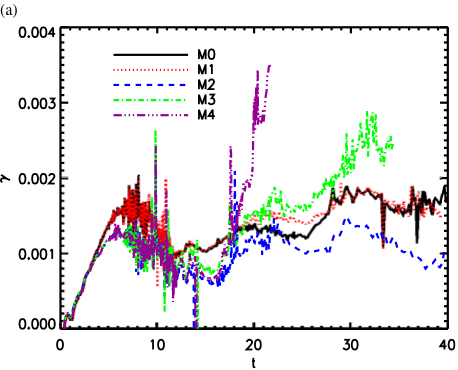
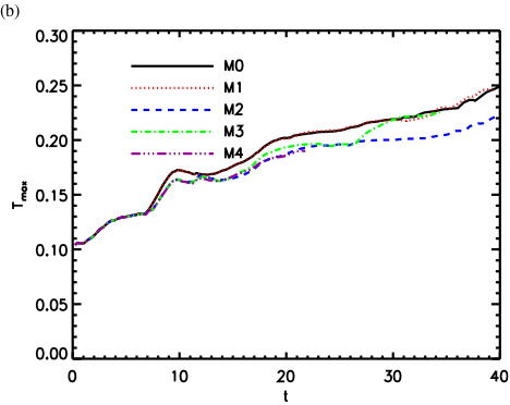
Figure 4: (a) The time-dependent reconnection rate in all five cases. (b) The time-dependent evolution of the maximum plasma temperature in the simulation domain in all five cases.

References

- Barta et al. (2011) Bárta, M., Büchner, J., Karlicky, M., & Kotrc, P., ApJ, 730, 47, 2011.
- Bhattacharjee et al. (2009) Bhattacharjee, A., Huang, Y.-M., Yang, H., & Rogers, B., Phys. Plasmas, 16, 112102, 2009.
- Biskamp (1986) Biskamp, D., Phys. Fluids, 29, 1520, 1986.
- Botha et al. (2011) Botha, G. J. J., Arber, T. D., & Hood, A. W., A&A, 525, A96, 2011.
- Buchner & Elkina (2006) Büchner, J., & Elkina, N., Phys. Plasmas, 13(8),082304.I-082304.9, 2006.
- Chen et al. (1999) Chen, P. F., Fang, C., Ding, M. D., & Tang, Y. H., ApJ, 520, 85, 1999.
- Guo et al. (2012) Guo, Z.B., Diamond , P.H., & Wang, X.G., has been submitted to ApJ, 2012.
- Huang et al. (2010) Huang, Y.-M., & Bhattacharjee, A., Phys. Plasmas, 17, 062104, 2010.
- Isobe & Shibata (2009) Isobe, H., & Shibata, K., Journal of Astrophysics and Astronomy, Volume30, 79-85, 2009.
- Lin et al. (2005) Lin, J., Ko, Y.-K., Sui, L., Raymond, J. C., Stenborg, G. A., Jiang, Y., Zhao, S., & Mancuso, S., ApJ, 622, 1251, 2005.
- Lin et al. (2008) Lin, J., Cranmer, S. R., & Farrugia, C. J., JGRA, 113, 11107, 2008.
- Mei et al. (2012) Mei, Z., Shen, C., Wu, N., Lin, J., Murphy, N. A., & Roussev, I. I., MNRAS, submitted, 2012.
- Milligan et al. (2010) Milligan, R. O., McAteer, R. T. J., Dennis, B. R., & Young, C. A., ApJ, 713, 1292, 2010.
- Nagashima & Yokoyama (2006) Nagashima, K., & Yokoyama, T., ApJ, 647:654-661, 2006.
- Ni et al. (2010) Ni, Lei, Germaschewski, Kai, Huang, Yi-Min, Sullivan, Brian. P., Yang, Hongang, & Bhattacharjee, A., Phys. Plasmas, 17, 052109, 2010.
- Ni et al. (2012) Ni, Lei, Ziegler, Udo, Huang, Yi-Min, Lin, Jun, & Mei, Zhixing, Phys. Plasmas, Phys. Plasmas, 19, 072902, 2012.
- Nishikawa & Neubert (1996) Nishikawa, K.-I., & Neubert, T., Adv. Space Res., 18, 263, 1996.
- Nishizuka et al. (2010) Nishizuka, N., Takasaki, H., Asai, A., & Shibata, K., ApJ, 711, 1062, 2010.
- Priest & Forbes (2000) Priest, E. R., & Forbes, T. G., Magnetic Reconnection: MHD theory and applications, Cambridge University Press, Cambridge, 2000.
- Roussev et al. (2002) Roussev, I., Galsgaard, K., & Judge, P.G., A&A, 382, 639-649, 2002.
- Savage et al. (2010) Savage, S. L., McKenzie, D. E., Reeves, K. K., Forbes, T. G., & Longcope, D. W., ApJ, 722, 329, 2010.
- Schmidt (1966) Schmidt, G., Physics of High-Temperature Plasmas, Academic Press, London, 1966.
- Shen et al. (2011) Shen, C., Lin, J., & Murphy, N. A., ApJ, 737, 14, 2011.
- Spitzer (1962) Spitzer, L., Physics of Fully Ionized Gases, Interscience, New York, 1962.
- Takaaki & Kazunari (1997) Takaaki, Y., & Shibata, K., Magnetic Reconnection in the Solar Atmosphere, ASP Conference Series, 111, 1997.
- Ziegler (2008) Ziegler, U., Comp. Phys. Commun.,179, 227, 2008.