Convex Regularization of Local Volatility Estimation in a Discrete Setting

Abstract

We apply convex regularization techniques to the problem of calibrating the local volatility surface model of Dupire taking into account the practical requirement of discrete grids and noisy data. Such requirements are the consequence of bid and ask spreads, quantization of the quoted prices and lack of liquidity of option prices for strikes far way from the at the money level.

We obtain convergence rates and results comparable to those obtained in the idealized continuous setting. Our results allow us to take into account separately the uncertainties due to the price noise and those due to discretization errors. Thus allowing better discretization levels both in the domain and in the image of the parameter to solution operator.

We illustrate the results with simulated as well as real market data. We also validate the results by comparing the implied volatility prices of market data with the computed prices of the calibrated model.

Keywords: Convex regularization, local volatility surfaces, regularization convergence rates, numerical methods for volatility calibration.

AMS subject classifications: 91G60 (65M32 91B70)

1 Introduction

During the last two decades we have witnessed an explosion of interest on mathematical models in Finance. Indeed, the need for tools to understand risk and volatility in equity and commodity prices is crucial for the financial industry. A well accepted class of models consists of an extension of the Black-Scholes model known as local-volatility models. It was pioneered by B. Dupire in [22] for the continuous case and has been a standard in many financial applications.

Local volatility models subsume that the volatility coefficient in the stochastic differential equation that determines the dynamics of the underlying is a function of time and of the underlying at that time. The calibration of such surface becomes fundamental for the consistent pricing of more complex derivatives.

In this article we are concerned with the calibration of local-volatility models from option market data in a realistic setting that incorporates the availability of noisy and discrete financial data. Mathematically, it is connected to the identification of a (nonconstant) diffusion coefficient in a parabolic equation. It is well known that such calibration problem, as many important ones in Mathematical Finance, is highly ill-posed. In particular, small changes and noise in the data may lead to substantial changes in the results. Yet, good volatility surface calibration is crucial in a plethora of applications, including risk management, hedging, and the evaluation of exotic derivatives. In order to tackle the ill-posedness of the calibration we make use of (non quadratic) Tikhonov-type regularization techniques and extend previous work [19, 20]. More precisely, we extend the results presented in [19, 20] for a discrete setting, under less restrictive assumptions than the ones used in [37].

The introduction of regularization techniques in order to stabilize the problem leads to a crucial question: If the noise in the data goes to zero, does the corresponding regularized solution converge to the true volatility? If this is the case, it would be also natural to inquire about the rate of convergence.

In the sequel, we shall respond such questions by recalling some results present in literature [17, 18, 19]. Such results concern existence and stability of the regularized solutions as well as convergence and convergence rate in terms of the noise level.

The novelty and main contributions of the present article

While keeping the underlying model in a context of partial differential equations and continuous variables, we apply a discretization process that determines the level of regularization in the coarse grid associated to the available data. This brings the problem from a context of infinite dimensional identification to a finite dimensional one in a regularized way. At this point, our contribution is the proof of results concerning the regularizing properties of finite dimensional solutions, the noise level and the levels of discretization in the range and in the domain of the forward operator. In particular, the convergence rate result, under this setting, shows that there is an intrinsic relation between the level of discretization in the domain and the noise of the observed prices. More precisely, given the noise level and the level of discretization in the range of the forward operator, there is an optimal level of discretization in the domain $\mathcal{D}(F)$ of $F$ that minimizes the distance between the regularized solution and the true local volatility surface.

It can be intuitively interpreted as follows:
If we use very few elements in the discretization of ${\cal D}({F})$, the resulting surface could not capture the variability of the original local volatility, i.e., the regularized solution would be almost constant. On the other hand, if we use too many elements, the inverse problem would be under-determined. Thus, given the level of uncertainties associated to the data, there should be an optimal choice for the discretization level of ${\cal D}({F})$.
This can be seen as a discrepancy principle w.r.t the level of discretization in the domain of $F$. Therefore, choosing an appropriate level of discretization in the domain of the operator $F$ is crucial for achieving reliable solutions. One way of obtaining this is by accounting separately for the uncertainty contributions in the discretization levels for the domain and image, and the noise level from market bid and ask spread when implementing the inverse problem analysis. The convergence rate result in Section 3, is, in certain sense, a theoretical evidence of this feature, since it states how distant, in an appropriate sense, a reconstructed local volatility surface is from the true solution in terms of the three quantities above mentioned.

This discrete setting gives us sufficient conditions to explore better the third main point of the present work, the numerical implementation of different regularization approaches, that allows us to illustrate the theoretical results presented in Section 3. This contribution is presented in Section 4.

The Setting and the Inverse Problem:

We are concerned with the problem of local volatility calibration from European call options. Different versions of the calibration problem have been addressed by many authors using techniques different from those described here. See [1, 6, 7, 8, 9, 10, 11, 12, 16, 21, 24, 27, 28, 29, 30, 33, 34, 35, 42].

We recall that, an European call is a contract that gives the right, but not the obligation, of paying a fixed amount, known as strike price, for one share of its underlying asset at maturity. To price such contract in the context of complete markets, we consider a filtered probability space $(\Omega,\mathcal{G},\mathbb{F},\mathbb{Q})$, where $\mathbb{F}$ is a filtration and $\mathbb{Q}$ is the risk neutral measure. Denote by $S_{t}=S(t,\omega)$, with $\omega\in\Omega$ and $t>0$, the price at time $t$ of the above mentioned asset. We assume that $S_{t}$ follows the Itô’s dynamics

$$dS_{t}=rS_{t}dt+\sqrt{\nu_{t}}S_{t}dW^{\mathbb{Q}}_{t},~{}~{}~{}t>0,~{}~{}~{}S(0)=S_{0}>0,$$ (1)

where $W^{\mathbb{Q}}$ is a $\mathbb{Q}$-Brownian motion and $\nu_{t}$ is the stochastic volatility.

In the present context, the price at time $t$ of an European call with strike $K>0$ and maturity $T\geq t>0$, written on the asset $S_{t}$, can be represented as the discounted expectation of the payoff $\max\{0,S_{T}-K\}$ in the risk neutral measure $\mathbb{Q}$, i.e.,

$$C(t,S_{t},T,K)=\mathbb{E}^{\mathbb{Q}}\left[\left.\text{e}^{-r(T-t)}\max\left\{0,S_{T}-K\right\}\right|\mathcal{F}_{t}\right],$$ (2)

where $r\geq 0$ is the annualized risk free interest rate.

We assume that the volatility term in Equation (1) is a deterministic function of time and asset price:

$$\sqrt{\nu_{t}}=\sigma(t,S_{t}).$$ (3)

It follows that, when we fix the current time and the current stock price, by setting $t=0$ and $S(t=0)=S_{0}$, the option price $C=C(T,K)$, as a function of its maturity and strike, satisfies Dupire’s equation [22]. More precisely, making the change of variables $y=\log(K/S_{0})$ and $\tau=T-t$, and defining

$$u(\tau,y)=C(t+\tau,S_{0}\text{e}^{y})~{}~{}\text{ and }~{}~{}a(\tau,y)=\sigma^{2}(\tau,S_{0}\text{e}^{y})/2,$$

the option prices $u(\tau,y)$ satisfy:

$$\left\{\begin{array}[]{rcll}-u_{\tau}+a(u_{yy}-u_{y})-ru_{y}&=&0,&0<\tau\leq T,~{}y\in I\subset\mathbb{R}\\ \\ u(\tau=0,y)&=&S_{0}(\text{e}^{y}-1)^{+},&y\in I\subset\mathbb{R}\\ \\ \displaystyle\lim_{y\rightarrow-\infty}u(\tau,y)&=&S_{0},&0<\tau\leq T,\\ \\ \displaystyle\lim_{y\rightarrow+\infty}u(\tau,y)&=&0,&0<\tau\leq T,\end{array}\right.$$ (4)

where $I\subset\mathbb{R}$ is an interval. Note that $I$ may be unbounded.

Note that, in the present setup (1)-(4), local volatility is non-observable and determines the distribution of the underlying asset. Thus, developing reliable calibration methods for this quantity is crucial in a plethora of applications, such as, hedging strategies based on pricing exotic derivatives.

Denote by $D:=(0,T]\times I$ the domain of the definition of Equation (4). In order to address the volatility calibration problem in a general and rigorous manner, we define below the parameter-to-solution operator:

$$\begin{array}[]{rcl}F:{\cal D}({F})\subset H^{1+\varepsilon}(D)&\longrightarrow&L^{2}(D),\\ a&\longmapsto&F(a)=u(a)-u(a_{0})\end{array}$$ (5)

where ${\cal D}({F}):=\{a\in a_{0}+H^{1+\varepsilon}(D):\underline{a}\leq a\leq\overline{a}\}$, with $0<\underline{a}<\overline{a}$ constants and $a_{0}\in H^{1+\varepsilon}(D)$ given. This operator associates each local volatility $a\in{\cal D}({F})$ to the difference $u(a)-u(a_{0})$, where $u(a)$ and $u(a_{0})$ are the unique solutions for Problem (4) with local volatilities $a$ and $a_{0}$, respectively. The set $H^{1+\varepsilon}(D)$ with $\varepsilon\in(0,1]$ is a fractional Sobolev space [2]. We also assume that we observe the solutions of Problem (4) in $L^{2}(D)$.

Note that, originally a solution for Problem (4) is only locally summable. Thus, the introduction of $u(a_{0})$ in the definition of $F$ is necessary since $u(a)-u(a_{0})$ lies in $W^{1,2}_{p}(D)$. This is the space of functions with weak derivatives up to order one in time and up to order two in space, all them in $L^{p}(D)$. For results concerning the existence and uniqueness of solutions for Problem (4) and regularity properties of the operator defined in (5), see [16, 17, 24] and references therein.

As above mentioned, in this article we are concerned with the problem of calibrating the local volatility surface from traded European call option prices. This so-called inverse problem can be stated as:
Given a set of traded option prices $\widetilde{u}\in L^{2}(D)$, find the associated local volatility surface $a^{\dagger}\in{\cal D}({F})$ satisfying the following operator equation:

$$\widetilde{u}=F(a^{\dagger})+u(a_{0}).$$ (6)

One solution for this inverse problem was proposed by Dupire [22], where, under no-arbitrage conditions, we could find local volatility through the formula (in log-moneyness variables):

$$a(\tau,y)=\displaystyle\frac{ru_{y}-u_{\tau}}{u_{yy}-u_{y}}.$$ (7)

Unfortunately, this formula is not applicable in practice, since it implies in differentiating a noisy data, which is given in a sparse grid.

Note that, when stating Problem (6), we have assumed that the data $\widetilde{u}$ is known with infinite precision in the whole domain. In order to be more realistic, we consider that, when measuring the data we have some sources of uncertainties and noise, which arise specially from the sparsity of data, bid-ask spread, delays and interpolation. In addition, it is well known that the forward operator $F$, defined in (8), is compact. See [18, 19, 24]. It implies that small perturbations in the data may lead to substantial changes in the reconstructed solution. Therefore, we state the local volatility calibration problem in more mundane setting as follows:
Given the set of traded prices $u^{\delta}$, find its corresponding local volatility surface $a^{\dagger}\in{\cal D}({F})$ from the operator equation

$$u^{\delta}=\widetilde{u}+E=F(a^{\dagger})+u(a_{0})+E,$$ (8)

where $\widetilde{u}$ represents the unobservable noiseless data and $E$ is a quantity compiling and quantifying some of the uncertainties concerned with the model. The set of noiseless prices are associated to $a^{\dagger}\in{\cal D}({F})$ through Problem (6).

Denote by $\eta>0$ an upper bound for the magnitude of $E$. In what follows, we assume that $\eta$ is known a priori and $E$ satisfies:

$$\|\widetilde{u}-u^{\delta}\|_{L^{2}(D)}=\|E\|_{L^{2}(D)}\leq\eta.$$ (9)

In Section 3, we shall express $\eta$ in terms of the following three different quantities:

1. The discretization level on the domain of $F$, which we denote by $\gamma_{n}\geq 0$;

2. The discretization level on the range of $F$, which we denote by $\rho_{m}\geq 0$;

3. The noise level concerning the financial market uncertainties, which we denote by $\delta>0$, where $n$ and $m$ are, respectively, the number of elements in the discretization of the domain and range of $F$.

Notation, Definition and Assumptions

In the remaining part of this section we introduce some important assumptions and tools in order to proceed with the inverse problem analysis under the convex regularization framework [13, 19, 27, 38, 40].

Assumption 1.

The regularization functional $f_{a_{0}}:{\cal D}({f})\subset H^{1+\varepsilon}(D)\longrightarrow[0,\infty]$ is convex, proper and weakly lower semi-continuous. Its domain ${\cal D}({f})$ contains ${\cal D}({F})$.

Another important tool is the Bregman distance with respect to the functional $f_{a_{0}}$:

Definition 1.

Let the functional $f$ satisfy Assumption 1. For a given $a\in{\cal D}({f})$, let $\partial f(a)\subset H^{1+\varepsilon}(D)^{*}$ denote the sub-differential of the functional $f$ at $a$. We denote by

$${\cal D}(\partial f)=\{\tilde{a}:\partial f(\tilde{a})\neq\emptyset\}$$

the domain of the sub-differential $\partial f(a)$ [15]. The Bregman distance with respect to $\zeta\in\partial f(a_{1})$ is defined on ${\cal D}({f})\times{\cal D}(\partial f)$ by

$$D_{\zeta}(a_{2},a_{1})=f(a_{2})-f(a_{1})-\langle\zeta,a_{2}-a_{1}\rangle\;.$$

In particular, if $f$ is differentiable, $\zeta=f^{\prime}(\cdot)$.

It is also important to define the Fenchel conjugate:

Definition 2.

Let the functional $f$ satisfy Assumption 1. The function $f^{*}:H^{1+\varepsilon}(D)^{*}\to\mathbb{R}$ given by

$$f^{*}(x^{*}):=\sup_{x\in H^{1+\varepsilon}(D)}\{\langle x,x^{*}\rangle-f(x)\}$$

is called the Fenchel conjugate of $f$ [41].

Finally, the concept defined below is strongly related to the convergence rates results of Section 2:

Definition 3.

Let $1\leq q<\infty$ be fixed. The Bregman distance $D_{\zeta}(\cdot,\tilde{a})$ of $f:H^{1+\varepsilon}(D)\to\mathbb{R}\cup\{+\infty\}$ at $\tilde{a}\in\mathcal{D}_{B}(f)$ and $\zeta\in\partial f$ is said to be $q$-coercive with constant $\underline{c}>0$ if

$$D_{\zeta}(a,\tilde{a})\geq\underline{c}{\left\lVert a-\tilde{a}\right\rVert}^{q}_{H^{1+\varepsilon}(D)}\mbox{, }\quad\forall a\in{\cal D}({f}).$$ (10)

2 Convex Regularization: A Review of Literature on Local Volatility Calibration

It is well known, theoretically as well as in practice [19, 16, 24, 28, 27], that the local volatility calibration is a highly ill-posed inverse problem. In other words, small changes and noise in the data may lead to substantial changes in the reconstructions. Given the importance of good model selection for the volatility surface, a great amount of effort had been made in order to tackle the ill-posedness of the calibration [19, 16, 24, 28, 27, 29].

For notational simplicity we formulate this calibration problem in an infinite dimensional framework. Hereafter, we shall assume again that $D$ is a bounded subdomain of $\mathbb{R}^{2}$. Within this framework, we remark that ${\cal D}({F})\subset H^{1+\varepsilon}(D)\cap L^{\infty}_{>0}(D)\subset L^{1}(D)$, where $L^{\infty}_{>0}(D)$ is the set of functions that are (essentially) bounded from below and above by some positive constants.

Successful strategies to stabilize the problem are connected to the introduction of regularization techniques. In particular, many regularization techniques have been proposed in order to overcome the stability difficulties, e.g. [19, 16, 24, 28, 27] and references therein. The most common regularization strategy for volatility calibration in the literature includes entropy based regularization [10], or convex type regularization [19, 16, 24, 28, 27]. A unified approach of those Tikhonov-type regularization was derived in [19] by means of the minimization of the Tikhonov functional

$$\mathcal{F}_{\beta,u^{\delta}}(a):=\|F(a)-u^{\delta}\|^{2}_{L^{2}(D)}+\beta f_{a_{0}}(a)$$ (11)

over ${\cal D}({F})$. In (11), $\beta>0$ is the regularization parameter and $f_{a_{0}}(\cdot)$ is the regularization functional that is assumed to satisfy the Assumption 1. In particular, we have the following examples:

Example 2 (Standard Quadratic Regularization).

Here we consider:

$$f_{a_{0}}(a)={\left\lVert a-a_{0}\right\rVert}^{2}_{L^{2}(\Omega)}\;,$$ (12)

A particular example that we are interested in is the finite dimensional version of the Tikhonov-type functional (12) that reads as follows: Let $\{\phi_{n}\}$ be an orthonormal basis for $L^{2}(\Omega)$. Then, consider the minimization of the functional

$$a\longmapsto\mathcal{F}_{\beta,u^{\delta}}(a):={\left\lVert F(a)-u^{\delta}\right\rVert}_{L^{2}(\Omega)}^{2}+\beta\sum_{j=1}^{n}|\langle a-a_{0},\phi_{j}\rangle|^{2}\,.$$ (13)

This Tikhonov functional can be interpreted as a finite dimensional version of the quadratic regularization. In particular, this is an interesting penalization functional to consider in the discrete regularization approach in Section 3 and for numerical purposes in Section 4.

Example 3 (Kullback-Leibler Regularization).

Let us now consider:

$$f_{a_{0}}(a)={\text{KL}}({a_{0}},{a})\;,$$ (14)

where

$${\text{KL}}({a_{0}},{a})=\int_{D}a\log(a_{0}/a)-(a_{0}-a)\,dx\;\mbox{ .}$$

Note that the Kullback-Leibler distance is the Bregman distance associated to the Boltzmann-Shannon entropy

$${\cal G}(a):=\int_{D}a\log(a)\,dx\;.$$ (15)

One important motivation for convex regularization follows from the fact that, in some cases, if the sequence $\{a_{k}\}$ converges weakly to $a$ and also satisfies that $f_{a_{0}}(a_{k})\longrightarrow f_{a_{0}}(a)$ as $k\rightarrow\infty$ then it convergences strongly. This property is known as the Radon-Riesz, Kadec-Klee property, or yet H-property [45]. In particular, for locally uniformly convex and reflexive Banach spaces and some Besov spaces, such a property is fulfilled when $f_{a_{0}}={\left\lVert\cdot\right\rVert}^{p}$, for $1<p<\infty$. See [2, 25, 45]. Moreover, when we consider $L^{1}$ with its weak topology and $f_{a_{0}}$ as the Boltzmann-Shannon entropy, such property is satisfied. See [45].

Remark 1.

The domains of ${\cal G}$, ${\cal D}({{\cal G}})$, and of the subgradient of ${\cal G}$, ${\cal D}({\partial{\cal G}})$, are $L_{\geq 0}^{\infty}(D)$ (the set of bounded non-negative functions) and $L_{>0}^{\infty}(D)$, respectively.

The Kullback-Leibler distance, which is the Bregman distance of the Boltzmann-Shannon entropy, is defined on the Bregman domain ${\cal D}_{B}({\cal G})$, that is a subset of $L_{>0}^{\infty}(D)$. Moreover, the Kullback-Leibler distance is lower semi-continuous with respect to the $L^{1}$-norm [39]. Based on this property we extend the Kullback-Leibler distance, to take value $+\infty$ if either $a\notin{\cal D}({\cal{G}})$ or $b\notin{\cal D}_{B}({\cal G})$.

Note that, there are exceptional cases, when the integral

$$\int_{D}a\log(a/a_{0})-(a-a_{0})\,dx$$

is actually finite, but ${\text{KL}}({a},{a_{0}})=\infty$. This can be seen by taking for instance $a\in L_{>0}^{1}(D)$ which is not in $L^{\infty}(D)$ and $a_{0}=Ca$, where $C$ is a constant. The reason here, is that $a$ is not an element of the subgradient of the Boltzmann-Shannon entropy. This follows directly from the definition of the domain of the convex functionals and their subgradients.

2.1 Stability and Convergence

In this section we shall present the result on well-posedness, stability and convergence of minimizers of the Tikhonov functional $\mathcal{F}_{\beta,u^{\delta}}$ defined in (11).

Consider the forward operator $F$ defined in (8) and the spaces $H^{1+\varepsilon}(D)$ and $L^{2}(D)$ with its weak topologies. It follows from [19] that for any $\beta>0$ and $u^{\delta}\in L^{2}(D)$, there exists a minimizer of $\mathcal{F}_{\beta,u^{\delta}}$. In other words, the regularized problem has a solution. In addition, we have that such minimizers are stable in the following sense: If $(u_{k})$ is a sequence converging to $u$ in $L^{2}(D)$ with respect to the norm topology, then every sequence $(a_{k})$ with

$$a_{k}\in\text{argmin}\bigl{\{}\mathcal{F}_{\beta,u_{k}}(a):a\in{\cal D}\bigr{\}}$$

has a subsequence which converges weakly. The limit of every weak convergent subsequence $(a_{k^{\prime}})$ of $(a_{k})$ is a minimizer $\tilde{a}$ of $\mathcal{F}_{\beta,u}$. We also have that, when the noise level vanishes, the regularized solutions converge to the true local volatility surface in the following sense: Let also the map $\beta:(0,\infty)\to(0,\infty)$ satisfy

$$\beta(\delta)\to 0\text{ and }\delta^{2}/\beta(\delta)\to 0\,,\text{ as }\delta\to 0\;.$$

Moreover, let the sequence $(\delta_{k})$ converge to $0$. Assume that $(u_{k})$ with $u_{k}:=u^{\delta_{k}}$ is a sequence in $L^{2}(D)$ satisfying ${\left\lVert\bar{u}-u_{k}\right\rVert}\leq\delta_{k}$. Set $\beta_{k}:=\beta(\delta_{k})$. Then, every sequence $(a_{k})$ of minimizers of $\mathcal{F}_{\beta_{k},u_{k}}$, has a subsequence $(a_{k^{\prime}})$ converging weakly. Each limit $a^{\dagger}$ of such subsequences is an $f_{0}$-minimizing solution of (8), i.e., a solution of (8) that is a minimum of $f_{a_{0}}(\cdot)$. In other words, when the uncertainty level $\delta$ goes to zero and the parameter of regularization $\beta=\beta(\delta)$ is properly chosen, then the approximate solutions converge to the solution of (8). An illustration of this theorem is given in Section 4.

From the above discussion it is easy to see that the convex Tikhonov-type functional defined in Example 2 has stable minimizers that converge to the true local volatility surface when the noise level vanishes. However, for the Kullback-Leibler regularization approach of Example 3, it is necessary to make additional assumptions. Indeed, in order to state the convergence analysis for the Kullback-Leibler regularization, it is necessary to consider the weak-to-weak convergence of the forward operator (see Theorem 9 item (ii)) combined with the following inequality [39],

$${\left\lVert a-b\right\rVert}^{2}_{L^{2}(\Omega)}\leq 2^{-1}KL(a,b)\qquad\forall a,b\in\mathcal{D}(\mathcal{G})\,.$$ (16)

It guarantees the closedness of the graph of the Tikhonov functional (14) with Kullback-Leibler regularization. See [19, Theorem 27].

2.2 Convergence Rates

Under the same assumptions of the previous sections, we now recall a convergence rate result for the regularized solutions in terms of the noise level $\delta$. Such estimate is based on a prior knowledge about the true solution. This is the so-called source condition [26]. By [19, Lemma 14], for this specific problem, we can guarantee the existence of $w\in L^{2}(D)^{*}$ and $r\in H^{1+\varepsilon}(D)^{*}$ such that, the following approximated source condition holds

$$\zeta^{\dagger}=F^{\prime}(a^{\dagger})^{*}w+r\qquad\mbox{for}\qquad\zeta^{\dagger}\in\partial f(a^{\dagger})\,.$$ (17)

Consider the forward operator $F$ defined in (8). Let the source condition (17) be satisfied with $w^{\dagger}$ and $r$ such that

$$\big{(}\underline{c}\|w^{\dagger}\|_{L^{2}(D)}+\|r\|_{L^{2}(D)}\big{)}:=\beta_{1}\in[0,1).$$

Let also the Bregman distance with respect to $f_{a_{0}}$ be $q$-coercive with constant $\underline{c}\geq e^{-2}$, as in Definition 3. Moreover, let $\beta:(0,\infty)\to(0,\infty)$ satisfy $\beta(\delta)\sim\delta$. Then, by [19, Theorem 12 and Lemma 16], it follows that

$$D_{\zeta^{\dagger}}(a_{\beta}^{\delta},a^{\dagger})=\mathcal{O}(\delta)\,,\quad\left\|F(a^{\delta}_{\beta})-u^{\delta}\right\|_{L^{2}(D)}=\cal O(\delta)\;,$$

and there exists $c>0$, such that $f(a_{\beta}^{\delta})\leq f(a^{\dagger})+\delta/c$ for every $\delta$ with $\beta(\delta)\leq\beta_{\text{max}}$. Thus, the results concerning the existence and stability of regularized solutions added to the convergence and convergence rate results imply the H-property of Remark 3. The latter, in turn, depends on the uncertainty level.

Note that the $q$-coercivity assumption of the Bregman distance implies that

$${\left\lVert a_{\beta}^{\delta}-a^{\dagger}\right\rVert}_{H^{1+\varepsilon}(D)}=\mathcal{O}((\delta)^{\frac{1}{q}})\;.$$ (18)

In particular, for the Kullback-Leibler regularization we have [19] (according to the choice of $f_{a_{0}}$):

$${\left\lVert a^{\delta}_{\beta}-a^{\dagger}\right\rVert}_{L^{2}(D)}=\mathcal{O}(\sqrt{\delta})\qquad\mbox{or}\qquad{\left\lVert a^{\delta}_{\beta}-a^{\dagger}\right\rVert}_{L^{1}(D)}=\mathcal{O}(\sqrt{\delta})\,.$$ (19)

In the next section we address the regularization of the volatility calibration problem in a discrete setting, providing convergence and convergence rates results in terms of the noise level and the discretization levels in domain and range of the forward operator.

3 The Discrete Setting

In order to obtain more practical error estimates for the numerical solution of the Inverse Problem (8), we analyze the Tikhonov-type regularization presented in Section 2 in a discrete setting. The discreteness is modeled by considering fixed nested sequences of finite-dimensional subspaces of $H^{1+\varepsilon}(D)$ and $L^{2}(D)$ respectively, $\{U_{n}\}^{\infty}_{n=0}$ and $\{V_{m}\}^{\infty}_{m=0}$ such that $\overline{\cup^{\infty}_{n=0}U_{n}}=H^{1+\varepsilon}(D)$ and $\overline{\cup^{\infty}_{m=0}V_{m}}=L^{2}(D)$. Now, define the sets $\mathcal{D}_{n}=U_{n}\cap\mathcal{D}(F)$ for $n\in\mathbb{N}$ and assume that they are nonempty.

We can now define the operators $F_{m}:\mathcal{D}(F)\subset H^{1+\varepsilon}(D)\longrightarrow V_{m}$ approximating $F$ and a discrete version of the parameter $a\in\mathcal{D}(F)$, that we call $a_{n}\in\mathcal{D}_{n}$, satisfying

$$\|F(a)-F_{m}(a)\|_{L^{2}(D)}\leq\rho_{m},\quad{\left\lVert a_{n}-a\right\rVert}_{H^{1+\varepsilon}(D)}\leq\gamma_{n}\,,$$ (20)

with $\lim_{m\rightarrow\infty}\rho_{m}=0$ and $\lim_{n\rightarrow\infty}\gamma_{n}=0$ for all $a\in\mathcal{D}(F)$. In the numerical experiments of Section 4, the spaces $U_{n}$ are generated by finite sets of finite element functions and the operators $F_{m}$ are suitable finite difference operators associated to the Problem (4).

In this setting the discrete version of the Tikhonov-type calibration inverse problem takes the form:

Find a solution for the minimization problem of the following Tikhonov functional

$$\mathcal{F}_{\beta,u^{\delta}}^{m,n}:=\|F_{m}(a)-u^{\delta}\|^{2}_{L^{2}(D)}+\beta f(a)\quad\mbox{subject to a }\,\in\mathcal{D}_{n},$$ (21)

where $u^{\delta}$ is a prices surface satisfying Equation (9).

As in Section 2, we use convex regularization techniques to ensure the existence, stability of solution and convergence rates of the approximate solution sequence of the inverse problem.

We remark that, in the discrete setting we account separately for the uncertainties originated by the discretization of the operator $F$ and its domain of definition, and the noise introduced by the market noise such as bid and ask spread.

We start with the following auxiliary lemma:

Lemma 4.

• For all $m\in\mathbb{N}$, the finite difference operator $F_{m}$ is sequentially weakly closed.

• For every $M>0,\beta>0$ and $m,n\in\mathbb{N}$, the sets $\{a\in\mathcal{D}(F)\,:\,\mathcal{F}_{\beta,u^{\delta}}(a)\leq M\}$ and $\{a\in\mathcal{D}_{n}(F)\,:\,\mathcal{F}_{\beta,u^{\delta}}^{m,n}(a)\leq M\}$ are sequentially weakly compact.

Proof.

Item i) follows from the weak sequential continuity of $F$ (see [17, Chapter 1]) and definition of the finite different methods [44]. To prove Item ii), we recall that, by definition, $\mathcal{D}(F)$ and $\mathcal{D}_{n}(F)$ are convex and closed. Hence, weakly closed. Therefore, coercivity and weak semi-continuity of $f_{a_{0}}$ and Item i) conclude the proof. ∎

We are now ready to present the analysis of the a priori choice of the regularization parameter $\beta$.

3.1 A Priori Choice for the Regularization Parameter

In this subsection, we state the well-posedness and perform a convergence analysis of the discrete version of the calibration problem using the Tikhonov functional of Equation (21).

Proposition 5.

Let $m,n\in\mathbb{N}$ and $\beta,\delta>0$ be fixed. Moreover, let (9) be satisfied. Then, for every $u^{\delta}\in L^{2}(D)$, there exists at least one minimizer of (21).

Furthermore, the minimizers of (21) are stable with respect to the data $u^{\delta}$ in the sense of Section 2.1

The proof is straightforward by the standard arguments presented in [43, Theorem 3.23] and [37, Proposition 2.3] jointly with Lemma 4 and the assumptions on $f_{a_{0}}$.

We prove now the auxiliary lemma:

Lemma 6.

Assume that an $f_{a_{0}}$-minimizing solution $a^{\dagger}$ belongs to the interior of $\mathcal{D}(F)$. Moreover, let $\rho>0$ be small enough so that the closed ball $B_{\rho}(a^{\dagger})$ is in the interior of $\mathcal{D}(F)$. Assume that $a_{n}\in\mathcal{D}_{n}(F)\cap B_{\rho}(a^{\dagger})$, for $n$ sufficiently large, satisfying (20).

Then, $f_{a_{0}}(a_{n})\longrightarrow f_{a_{0}}(a^{\dagger})$ as $n\rightarrow\infty$.

Proof.

Since $\mathcal{D}(F)$ is convex and closed, the convexity and weak lower semi-continuity of $f_{a_{0}}$ implies that $f_{a_{0}}$ is lower semi-continuous [25, Corolary 2.2]. Assumption 20 implies that $a_{n}\rightarrow a$ as $n\rightarrow\infty$. Now, [25, Corolary 2.5] implies that $f_{a_{0}}$ is continuous in the interior of $\mathcal{D}(F)$. ∎

The next theorem ensures that the minimizing solutions of Equation (21) are also regularized solutions of Equation (8), given a suitable choice for the regularization parameter when $m,n\rightarrow\infty$. We remark that in [37] a similar result was obtained. However they need to assume stronger conditions. One of the main differences between our proof and that in [37] is the validity of the tangential cone condition in our case. Such condition is reviewed in Theorem 11 of Appendix A.

Theorem 7.

Let (9), (20) and the assumptions on Lemma 6 be satisfied. Moreover, let $\beta=\beta(\rho_{m},\gamma_{n},\delta)$ be such that

$$\beta\rightarrow 0\,,\qquad\frac{(\max(\rho_{m},\gamma_{n},\delta))^{2}}{\beta}\rightarrow 0\,,\qquad\mbox{as}\,\,\delta\rightarrow 0\,\,\mbox{and }\,\,m,n\rightarrow\infty\,.$$

Then, every sequence $\{a_{k}\}_{k\in\mathbb{N}}$, with $a_{k}:=a_{m_{k},n_{k}}^{\beta_{k},\delta_{k}}$ and $\beta_{k}:=\beta(\rho_{m_{k}},\gamma_{n_{k}},\delta_{k})$ such that $\delta_{k}\rightarrow 0$, $m_{k}\rightarrow\infty$, $n_{k}\rightarrow\infty$ as $k\rightarrow\infty$ and $a_{k}$ is a correspondent minimizer of (21), has a weakly convergent subsequence $\{a_{l}\}_{l\in\mathbb{N}}$ to an $f_{a_{0}}$-minimizing solution $a^{\dagger}$ of (8) and for which $\{f_{a_{0}}(a_{l})\}_{l\in\mathbb{N}}$ converges to $f_{a_{0}}(a^{\dagger})$. Moreover, if $a^{\dagger}$ is the unique solution of (8), then the entire sequence $\{a_{k}\}$ converges weakly to $a^{\dagger}$.

Proof.

(Sketch) We make use of standard arguments in the minimization theory of nonlinear Tikhonov regularization [43].

Let $a_{m,n}^{\beta,\delta}$ be a minimizer of (21) (the existence is guaranteed by Proposition 5). From the definition of $a_{m,n}^{\beta,\delta}$, it follows that

$$\begin{array}[]{rcl}{\left\lVert F_{m}(a_{m,n}^{\beta,\delta})-u^{\delta}\right\rVert}^{2}+\beta f_{a_{0}}(a_{m,n}^{\beta,\delta})&\leq&{\left\lVert F_{m}(a_{n})-u^{\delta}\right\rVert}^{2}+\beta f_{a_{0}}(a_{n})\\ &\leq&\left(\rho_{m}+{\left\lVert F(a_{n})-u\right\rVert}+\delta\right)^{2}+\beta f_{a_{0}}(a_{n})\,.\end{array}$$

From the continuity of $F$, the definition of $a_{n}$ and the tangential cone condition (see Theorems 9 and 11 in the Appendix A), we have

$${\left\lVert F_{m}(a_{m,n}^{\beta,\delta})-u^{\delta}\right\rVert}^{2}+\beta f_{a_{0}}(a_{m,n}^{\beta,\delta})\leq C(\max(\rho_{m},\gamma_{n},\delta))^{2}+\beta f_{a_{0}}(a_{n})\,.$$ (22)

Therefore,

$$f_{a_{0}}(a_{m,n}^{\beta,\delta})\leq C\frac{(\max(\rho_{m},\gamma_{n},\delta))^{2}}{\beta}+f_{a_{0}}(a_{n})\,.$$ (23)

Lemma 6 and the assumptions on $\beta$ guarantee that

$$\displaystyle\limsup_{\stackrel{{\scriptstyle\delta\rightarrow 0}}{{m,n\rightarrow\infty}}}f_{a_{0}}(a_{m,n}^{\beta,\delta})\leq f_{a_{0}}(a^{\dagger})\quad\mbox{and}\quad\displaystyle\lim_{\stackrel{{\scriptstyle\delta\rightarrow 0}}{{m,n\rightarrow\infty}}}{\left\lVert F_{m}(a_{m,n}^{\beta,\delta})-u\right\rVert}=0\,.$$ (24)

Let now $\beta_{k}:=\beta(\rho_{m_{k}},\gamma_{n_{k}},\delta_{k})$ and $a_{k}:=a_{m_{k},n_{k}}^{\beta_{k},\delta_{k}}$. Since $\{\mathcal{F}_{\alpha_{k},u^{\delta_{k}}}^{m_{k},n_{k}}(a_{k})\}$ is bounded, the coercivity of $f_{a_{0}}$ implies that $\{{\left\lVert a_{k}\right\rVert}\}$ is bounded. From Lemma 4, there exists a subsequence $\{a_{l}\}_{l\in\mathbb{N}}$ weakly convergent to some $\tilde{a}\in\mathcal{D}_{n}(F)$. Due to the weak lower semi-continuity of $f_{a_{0}}$ and (24), we get that

$$f_{a_{0}}(\tilde{a})\leq\liminf_{l\rightarrow\infty}f_{a_{0}}(a_{l})\leq\limsup_{l\rightarrow\infty}f_{a_{0}}(a_{l})\leq f_{a_{0}}(a^{\dagger})\,.$$

Continuity of $F$ implies that $F(\tilde{a})=u$. Therefore, $\tilde{a}$ is an $f_{a_{0}}$-minimizing solution of (8). ∎

3.2 Convergence Rates

We now state results concerning the convergence rates for the regularized solutions in the discrete setting. As in the continuous version presented in Section 2, we need some a priori knowledge about the true solution, which leads us to impose some source condition. Thus, we make use of the same source condition used in the continuous case, which is given by (17). Therefore, we are ready to prove the following theorem:

Theorem 8.

Suppose that $f_{a_{0}}$ satisfies the Definition 3. Let (9) and the source condition (17) be satisfied. If $\beta\sim\max(\rho_{m},\gamma_{n},\delta)$ and $\beta\beta_{2}<1$, then

$$D_{\zeta^{\dagger}}(a_{m,n}^{\beta,\delta},a^{\dagger})=\mathcal{O}(\max(\rho_{m},\gamma_{n},\delta))\,.$$ (25)

Proof.

Let $\{a_{n}\}_{n\in\mathbb{N}}$ be as in Theorem 7. From the definition of $a_{m,n}^{\beta,\delta}$ and estimate analogous to (3.1), it follows that

$${\left\lVert F_{m}(a_{m,n}^{\beta,\delta})-u^{\delta}\right\rVert}^{2}+\beta f_{a_{0}}(a_{m,n}^{\beta,\delta})\leq C(\max(\rho_{m},\gamma_{n},\delta))^{2}+\beta f_{a_{0}}(a_{n})\,.$$ (26)

Now, using (26) and the definition of the Bregman distance we have that

$${\left\lVert F_{m}(a_{m,n}^{\beta,\delta})-u^{\delta}\right\rVert}^{2} +\beta D_{\zeta^{n}}(a_{m,n}^{\beta,\delta},a_{n})$$

$$={\left\lVert F_{m}(a_{m,n}^{\beta,\delta})-u^{\delta}\right\rVert}^{2}+\beta\left(f_{a_{0}}(a_{m,n}^{\beta,\delta})-f_{a_{0}}(a_{n})-\langle\zeta^{n},a_{m,n}^{\beta,\delta}-a_{n}\rangle\right)\qquad$$

$$={\left\lVert F_{m}(a_{m,n}^{\beta,\delta})-u^{\delta}\right\rVert}^{2}+\beta f_{a_{0}}(a_{m,n}^{\beta,\delta})-\beta\left(f_{a_{0}}(a_{n})+\langle\zeta^{k},a_{m,n}^{\beta,\delta}-a_{n}\rangle\right)$$

$$\leq C(\max{\rho_{m},\gamma_{n},\delta})^{2}-\beta\langle\zeta^{k},a_{m,n}^{\beta,\delta}-a_{n}\rangle$$ (27)

$$=C(\max{\rho_{m},\gamma_{n},\delta})^{2}-\beta\langle\zeta^{k},a_{m,n}^{\beta,\delta}-a^{\dagger}\rangle-\beta\langle\zeta^{k},a^{\dagger}-a_{n}\rangle$$

$$=C(\max(\rho_{m},\gamma_{n},\delta))^{2}\underbrace{-\beta\langle\zeta^{k}-\zeta^{\dagger},a_{m,n}^{\beta,\delta}-a^{\dagger}\rangle}_{(A)}\underbrace{-\beta\langle\zeta^{\dagger},a_{m,n}^{\beta,\delta}-a^{\dagger}\rangle}_{(B)}$$

$$\qquad\quad\qquad\underbrace{-\beta\langle\zeta^{k}-\zeta^{\dagger},a^{\dagger}-a_{n}\rangle}_{(C)}\underbrace{-\beta\langle\zeta^{\dagger},a^{\dagger}-a_{n}\rangle}_{(D)}\,.$$

To conclude the proof, it remains to estimate the terms $(A)$, $(B)$, $(C)$ and $(D)$ in Equation (3.2) in terms of Bregman distance. At this point we will strongly use the existence of the source condition (17).

From [14, Lemma 1.3.9 iv)], it follows that

$$(A)\,\,=\,-\beta\left[D_{\zeta^{\dagger}}(a_{m,n}^{\beta,\delta},a^{\dagger})+D_{\zeta^{n}}(a^{\dagger},a_{n})-D_{\zeta^{n}}(a_{m,n}^{\beta,\delta},a_{n})\right]\,.$$ (28)

From the convergence rates of Section 2.2, it follows that

$$(B)\,\, \leq\beta|\langle\zeta^{\dagger},a_{m,n}^{\beta,\delta}-a^{\dagger}\rangle|\leq\beta\beta_{1}D_{\zeta^{\dagger}}(a_{m,n}^{\beta,\delta},a^{\dagger})+\beta\beta_{2}{\left\lVert F(a_{m,n}^{\beta,\delta})-F(a^{\dagger})\right\rVert}$$ (29)

$$\leq\beta\beta_{1}D_{\zeta^{\dagger}}(a_{m,n}^{\beta,\delta},a^{\dagger})+\beta\beta_{2}\left({\left\lVert F(a_{m,n}^{\beta,\delta})-F_{m}(a_{m,n}^{\beta,\delta})\right\rVert}+{\left\lVert F_{m}(a_{m,n}^{\beta,\delta})-u^{\delta}\right\rVert}+{\left\lVert u^{\delta}-F(a^{\dagger})\right\rVert}\right)\,.$$

Using Cauchy-Schwartz inequality, and the result in Reference [14, Proposition 1.1.7 ii)], it follows that

$$(C)\,\,\leq\beta{\left\lVert\zeta^{n}-\zeta^{\dagger}\right\rVert}{\left\lVert a_{n}-a^{\dagger}\right\rVert}\leq\beta C{\left\lVert a_{n}-a^{\dagger}\right\rVert}\,.$$ (30)

Finally, from the source representation (17) and the Lipschitz continuity of $F^{\prime}(a^{\dagger})$, we have that

$$(D)\,\, =\beta\left(\langle r-\zeta^{\dagger},a^{\dagger}-a_{n}\rangle+\langle r,a_{n}-a^{\dagger}\rangle\right)=\beta\left(\langle F^{\prime}(a^{\dagger})^{*}w,a^{\dagger}-a_{n}\rangle+\langle r,a_{n}-a^{\dagger}\rangle\right)$$

$$\leq\beta\left({\left\lVert w\right\rVert}{\left\lVert F^{\prime}(a^{\dagger})(a^{\dagger}-a_{n})\right\rVert}+{\left\lVert r\right\rVert}{\left\lVert a_{n}-a^{\dagger}\right\rVert}\right)\leq\beta\left(C{\left\lVert w\right\rVert}+{\left\lVert r\right\rVert}\right){\left\lVert a_{n}-a^{\dagger}\right\rVert}\,.$$ (31)

Putting together (3.2), and the estimates $(A)$, $(B)$, $(C)$ and $(D)$, the assumptions on the parameters and the fact that $D_{\zeta}(a,\tilde{a})\geq 0$, we get the conclusion. ∎

It is worth noticing that under different assumptions from the ones we have in Theorem 8, a similar result was proved in [37]. However, we have weaker assumptions than those in [37]. Moreover, all the assumptions are verified for the calibration problem under consideration.

Remark 2.

The estimate (25) accounts separately for the contributions of different sources of uncertainties. It improves the error estimates when performing numerical tests, making more reliable the solutions obtained by these techniques.

In particular, the estimate (25) implies an upper bound for the discretization level of $\mathcal{D}(F)$ w.r.t. the quality of the observation and the quantity of data. In other words, a discrepancy principle is obtained (as a function of the discretization level in $\mathcal{D}(F)$) at the first iteration for which $\rho_{m}\leq\max\{\gamma_{n},\delta\}$. This discrepancy principle will be verified numerically in Section 4. A rigorous proof is the subject of [4].

4 Numerical Results

We numerically solve the minimization problem in Equation (21) connected to Tikhonov regularization of the inverse problem of local volatility calibration. It is done by a gradient method. See [3, 5]. The direct problem of Equation (4), as well as, its related adjoint, arising in the calculation of the Tikhonov’s functional gradient, are numerically solved by a Crank-Nicholson scheme. See [3, 5, 17, 44]. Some of the theoretical statements of past sections, such as convergence analysis and rates as well as the proposed discrepancy principle in the choice of the discretization level, are now illustrated. We also present some reconstructions of the local volatility surface from traded option data.

4.1 Synthetic Examples

We generate the synthetic data of option prices as follows: We first choose a very fine mesh and calculate the option prices by the numerical solution of Problem (4) with the local volatility given in Equation (32). We apply to the resulting prices a zero-mean additive Gaussian white noise with variance $1\%$ of the maximum value of such option prices. Then, we choose the resulting perturbed data in a coarser grid contained in the first one. This is done in order to avoid the so-called inverse crime [32].

The local volatility surface used in the present set of numerical experiments is defined by:

$$\sigma(\tau,y)=\left\{\begin{array}[]{ll}\displaystyle\frac{2}{5}-\frac{4}{25}\text{e}^{-\tau/2}\cos\left(\displaystyle\frac{4\pi y}{5}\right),&\text{ if }-2/5\leq y\leq 2/5\\ \\ 2/5,&\text{ otherwise.}\end{array}\right.$$ (32)

Recall that the diffusion parameter of Problem 4 is $a=\sigma^{2}/2$. Note also that, Problem (4) is numerically solved in the domain $D=[0,1]\times[-5,5]$.

We choose the standard two-dimensional linear basis for the domain of the forward operator, since it is smooth. Such smoothness is a feature favored by practitioners [23]. In order to find its appropriate level of discretization, we also assume that the uncertainty levels $\delta$ and $\rho_{m}$ are given and proceed as follows:

1. Chose different meshes that correspond to different levels of discretization of $\mathcal{D}(F)$ with the spline basis. We require that the coarser mesh is contained in the finner one.

2. For each mesh, solve the inverse problem with the parameter of regularization $\beta$ chosen by the related Morozov’s discrepancy principle. See [5, 36].

3. Choose the coarser grid which satisfies the discrepancy criterion:

   $$\tau_{1}\max(\delta,\rho_{m})\leq\|F_{m}(a^{\beta,\delta}_{m,n})-u^{\delta}\|\leq\tau_{2}\max(\delta,\rho_{m}),$$ (33)

   where, $m$ and $\delta$ are fixed and $\tau_{1}$ and $\tau_{2}$ are given constants.

The intuitive justification of the above procedure is that:
If the level of discretization is too small, the reconstructed local volatility does not capture the variability of the original one. On the other hand, if we choose a level of discretization finer than necessary, we start to reproduce noise.
Such a conclusion can be partially motivated by the convergence rates of Theorem 8.

For the present examples, we chose $\tau_{1}=1.05$ and $\tau_{2}=1.5$. Furthermore, we consider that $\rho_{m}=0$, since we use a fine mesh in the numerical solution of Problem (4). Figure 1 illustrates the above mentioned discrepancy principle to find the appropriate level of discretization for ${\cal D}({F})$.

The data was generated using the step sizes, $\Delta t=0.0025$ and $\Delta y=0.01$. After adding noise, we collected the data in a mesh with step sizes $\Delta t=0.02$ and $\Delta y=0.1$. The direct problem in Equation (4) and its adjoint were numerically solved with $\Delta t=0.02$ and $\Delta y=0.1$. The reconstruction of Figures 1 and 2 were calculated with meshes in ${\cal D}({F})$ with the following step sizes:

$$\Delta t=0.1,0.08,0.07,0.06,0.05,0.04,0.03,0.02,0.01,0.0075,0.005,0.0025$$

and

$$\Delta y=0.1,0.08,0.07,0.06,0.05,0.04,0.03,0.02,0.01,0.0075,0.005,0.0025.$$

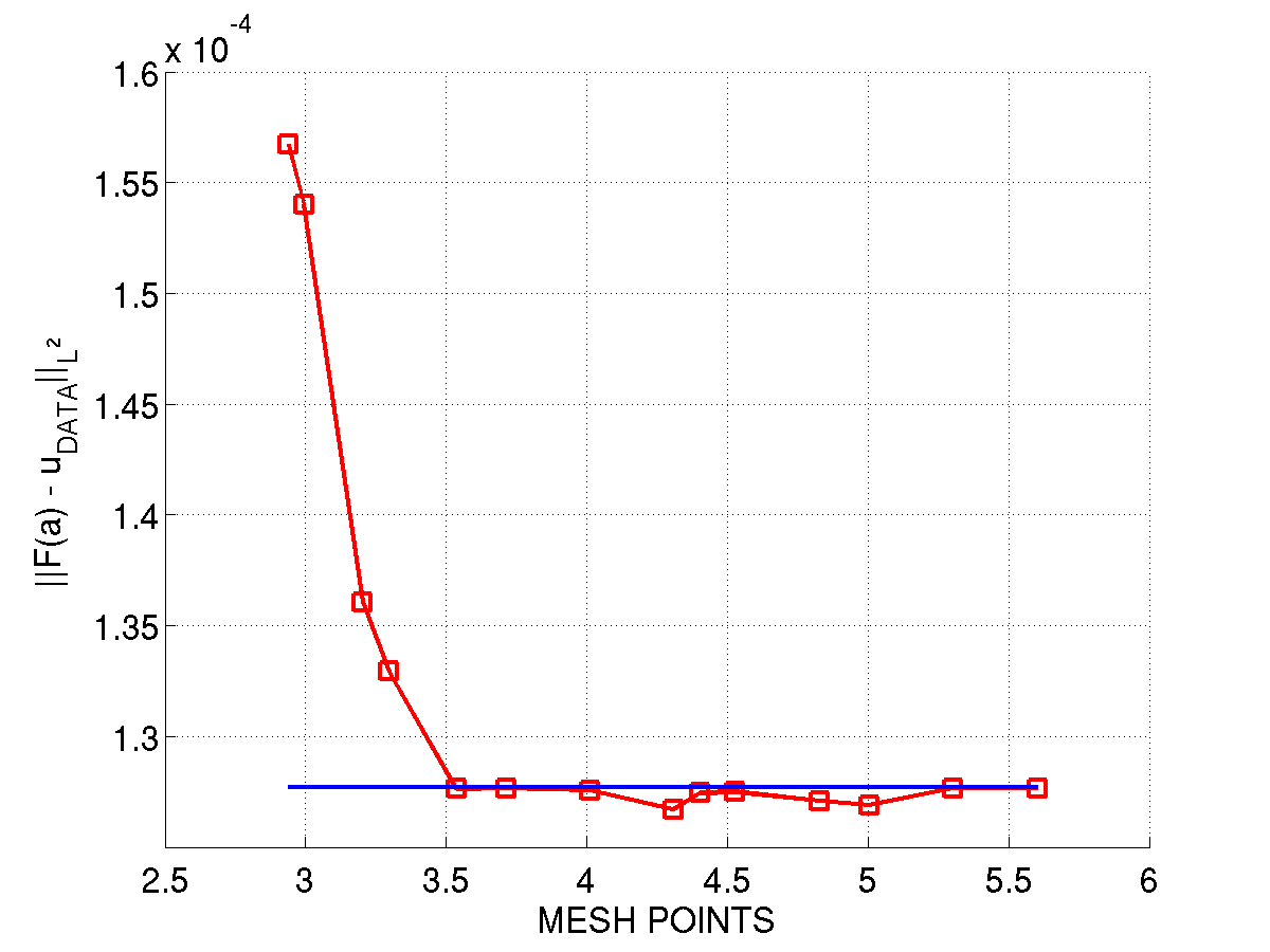
Figure 1: Evolution of the residual as a function of the number of mesh points. A discrepancy principle was used to find the appropriate level of discretization of $\mathcal{D}(F)$. In the presence of noise, its minimum is attained for a coarser mesh.The horizontal line corresponds to $\tau_{1}\delta$.

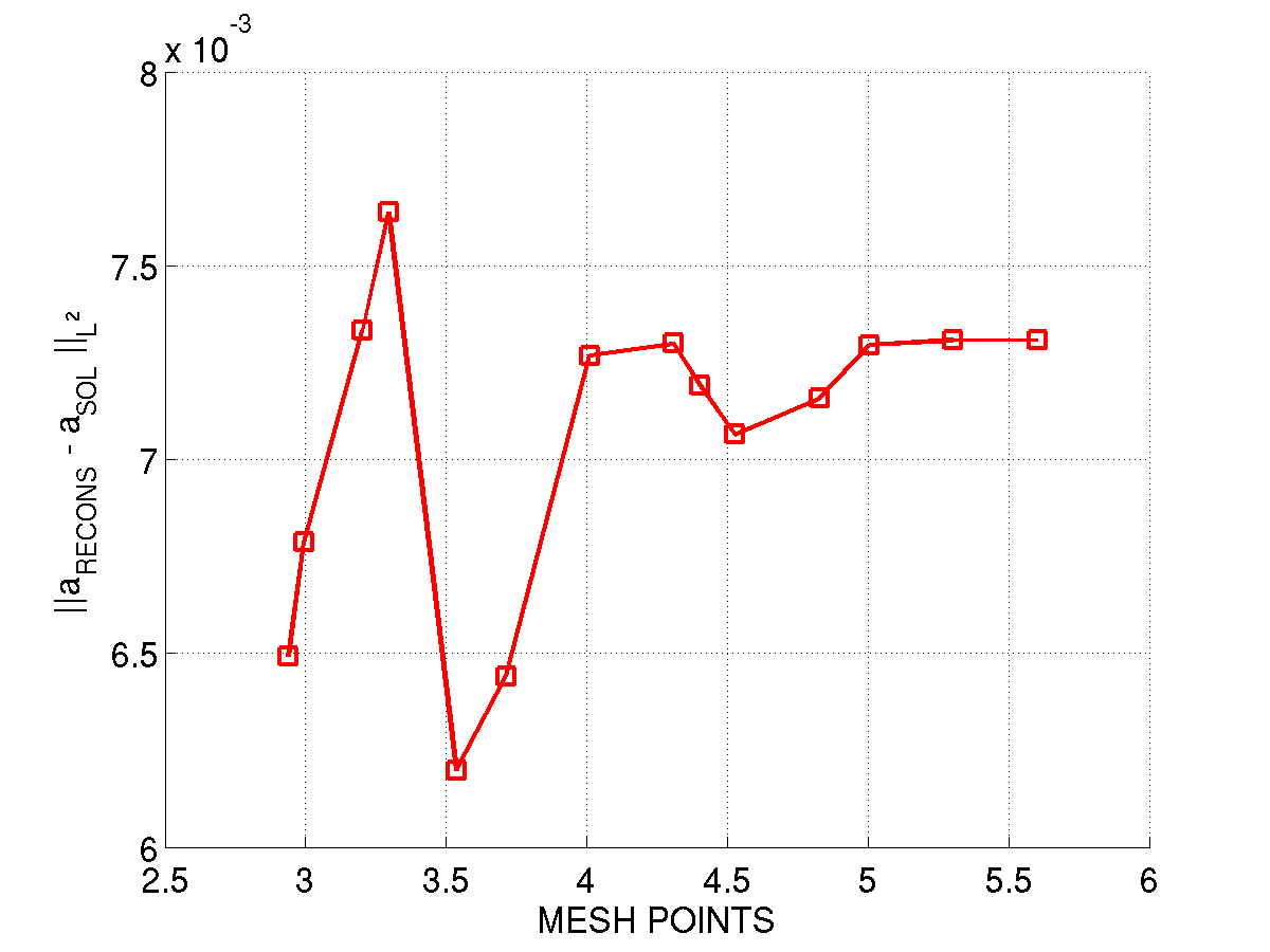
Figure 2: Evolution of the $L^{2}$-error. In the presence of noise, its minimum is attained for a coarser mesh.

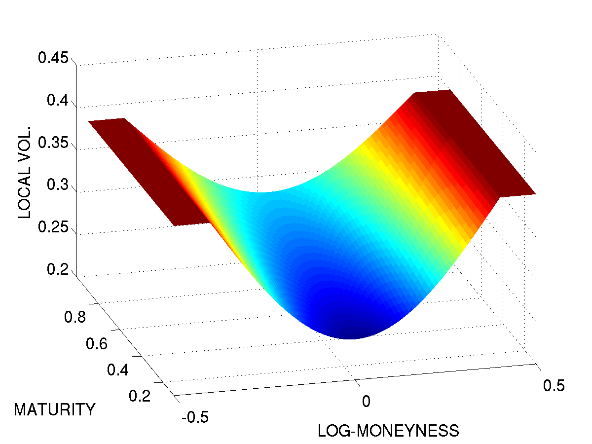
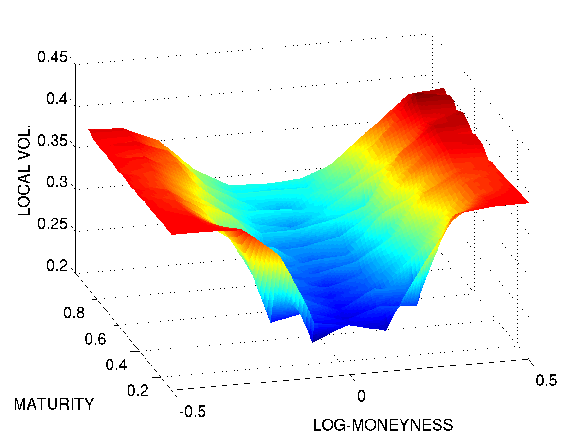
Figure 3: Left: original surface. Center and right: reconstructions corresponding to the first and second points satisfying the discrepancy principle of Figure 1, respectively.

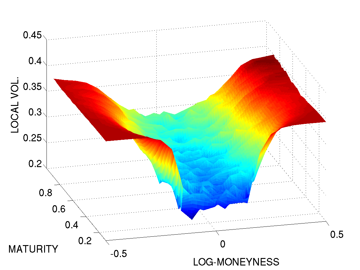
Figure 4: Left: original surface. Center and right: reconstructions satisfying the discrepancy principle of Figure 1.

We also calculate the $L^{2}$-error, i.e., the $L^{2}(D)$ distance between the regularized solution and the original local volatility surface. The resulting $L^{2}$-error for the regularized solutions used in Figure 1 can be found in Figure 2. Note that, as expected, the first two reconstructions satisfying the discrepancy principle above minimize the $L^{2}$-error, as we can see in Figures 1 and 2. It is an empirical evidence that the discrepancy principle in Equation (33) is a reliable way of finding the appropriate level of discretization of ${\cal D}({F})$.

We used the standard regularizing functional

$$f_{a_{0}}(a)=\|a-a_{0}\|^{2}_{H^{1}(D)},$$

since it imposes smoothness in both time and space variables. As mentioned above, smoothness is an expected feature of local volatility. We also performed some tests using Kullback-Leibler regularization.

Figures 3 and 4 present reconstructions of local volatility satisfying the discrepancy principle. Note that the reconstructions that first satisfy the discrepancy principle of Figure 1 present better $L^{2}$-errors (as expected). Moreover, we can see that the surfaces of Figure 3, as it has a smaller number of unknowns, is smoother than the surfaces of Figure 4.

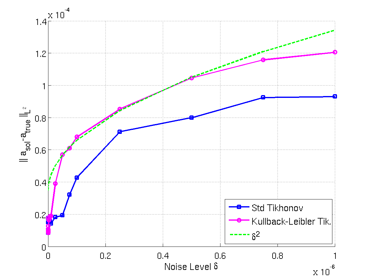
Figure 5: The $L^{2}$-error $r(\delta)=\|a_{\beta}(\delta)-a^{\dagger}\|_{L^{2}(D)}$ as a function of the noise level $\delta$ satisfies the convergence rates of Theorem 8. The dashed line is the function $g(\delta)=\sqrt{\delta}$.

One illustration of Theorem 8 is given in Figure 5, whereby, for different convex regularization approaches, we calculated the $L^{2}$-error as a function of the noise level $\delta$, as it goes to zero. Note that the estimates of Theorem 8 are satisfied. In this specific example, for simplicity, we kept $\rho_{m}$ and $\gamma_{n}$ constant.

4.2 Market Data: Henry Hub

We present below some reconstructions of the local volatility from call option prices on futures of the Henry Hub natural gas price traded in the CME stock exchange. In the present examples we use a uniform mesh with step sizes given by $\Delta t=0.005$ and $\Delta y=0.05$. We interpolate the data with a two-dimensional cubic spline. We also used a two-dimensional cubic spline basis for $\mathcal{D}(F)$ in the present set of experiments. We chose the appropriate discretization level for ${\cal D}({F})$ by the discrepancy principle of Equation (33).

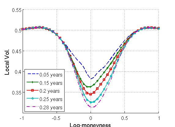
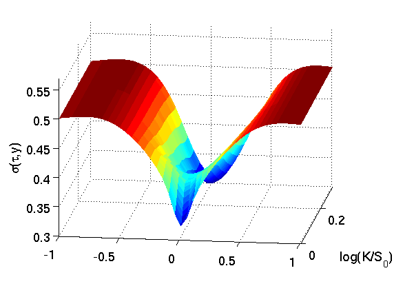
Figure 6: Left: Reconstructed local volatility for some fixed maturities. Right: Reconstructed local volatility surface.

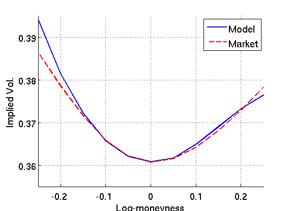
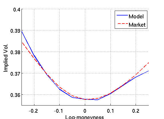
Figure 7: Implied (Black-Scholes) Volatility for market prices (dashed line) and prices generated by the reconstructed volatility of Figure 6 (continuous line)for two different maturities.

We used the standard $H^{1}(D)$ functional in these experiments with Tikhonov regularization, as in the above examples. It is important to note that, we used the traded price data as in [3, Chapter 4]. In the latter, the authors have assumed that option prices were given as a function of the unknown commodity spot price, instead of the underlying future prices.

Figure 6 presents the reconstructed local volatility for call option prices on Henry Hub future prices. Observe that the required smoothness is satisfied by the reconstructions. Figure 7 presents the implied volatility for the traded prices and the prices generated by the reconstructed local volatility surface of Figure 6 for two different maturities. Note that they become more similar as we get closer to the so-called “at-the-money” values, i.e., $y=0$. This turns out to be the region of the most liquid prices and thus less subjected to noise.

4.3 Market Data: S&P 500

The reconstructions of local volatility presented in Figures 8, 9, 10, 11 and 12 were obtained from call option prices on the S&P500 index traded at the NYSE on 05/09/2013. We used a uniform mesh with step sizes given by $\Delta t=0.005$ and $\Delta y=0.05$. We interpolate the data with the method proposed by N. Kahale in [31]. The main feature of this method is to avoid arbitrage opportunities by keeping the option prices convex functions of the strike. We also used a two-dimensional linear basis for $\mathcal{D}(F)$ in the present set of experiments. We chose the appropriate discretization level for ${\cal D}({F})$ by the discrepancy principle of Equation (33). Again, we used the standard $H^{1}(D)$ functional in the Tikhonov regularization.

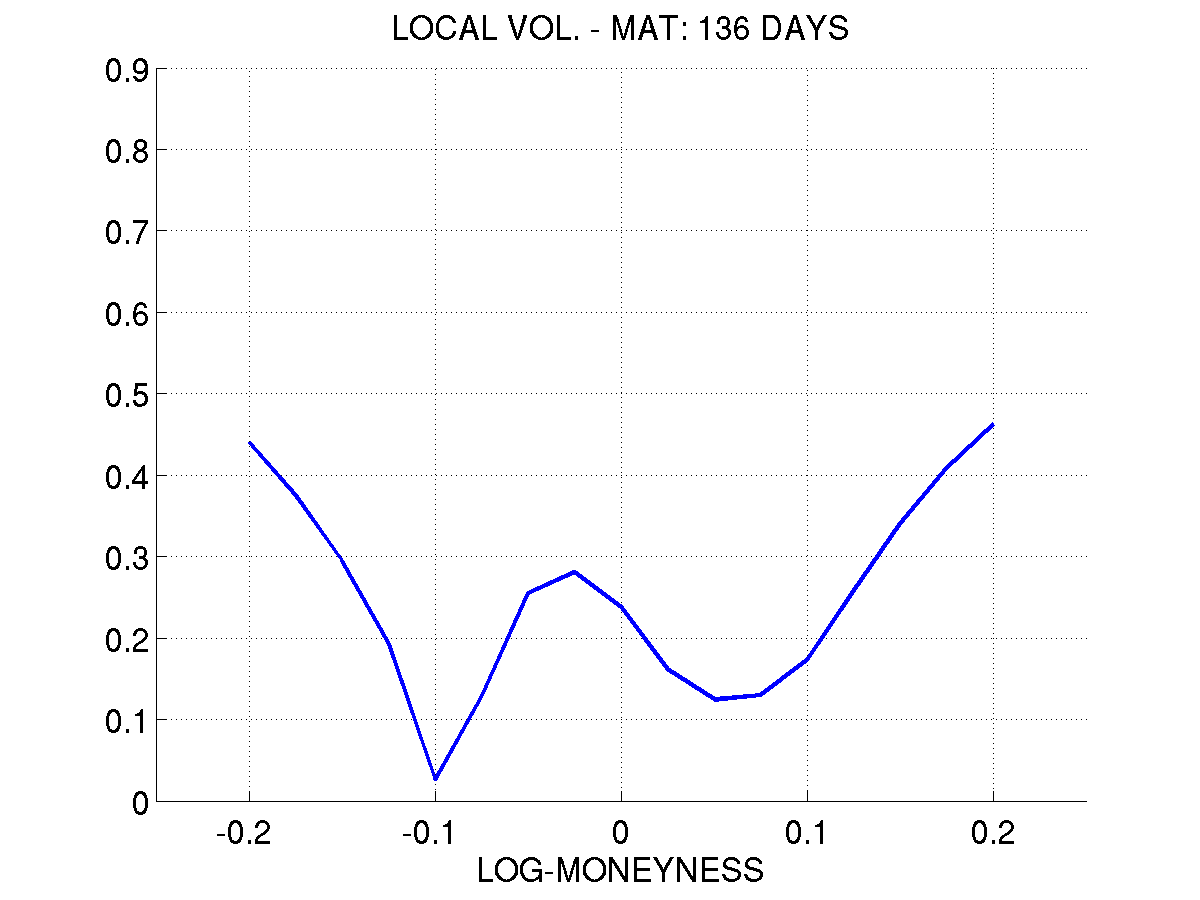
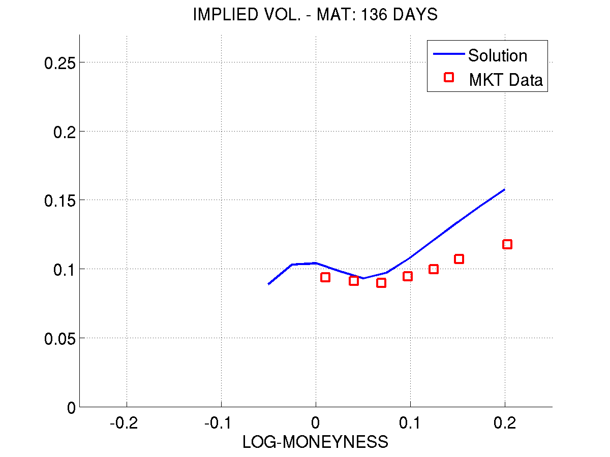
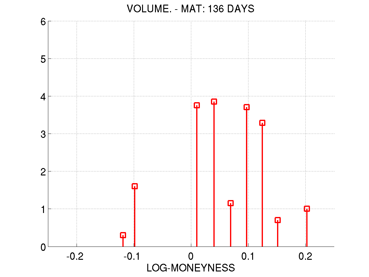
Figure 8: Left: Local volatility reconstructed from S&P500 call option prices traded on 05/09/2013 maturing on 09/21/2013. Center: Implied volatility of market data (squares) and implied volatility of the local volatility of the first figure (continuous line). Right: Volume of the prices used in this reconstruction in a $\log_{10}$ scale.

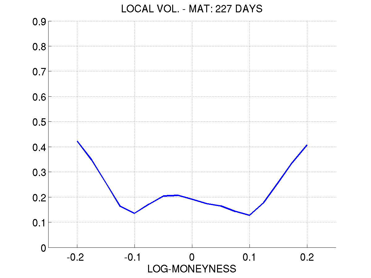
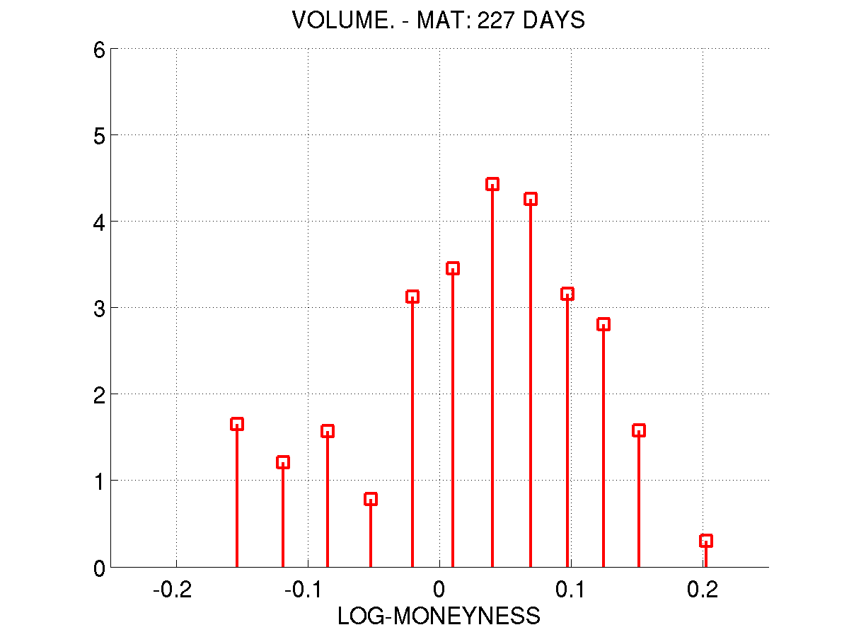
Figure 9: Left: Local volatility reconstructed from S&P500 call option prices traded on 05/09/2013 maturing on 12/21/2013. Center: Implied volatility of market data (squares) and implied volatility of the local volatility of the first figure (continuous line). Right: Volume of the prices used in this reconstruction in a $\log_{10}$ scale.

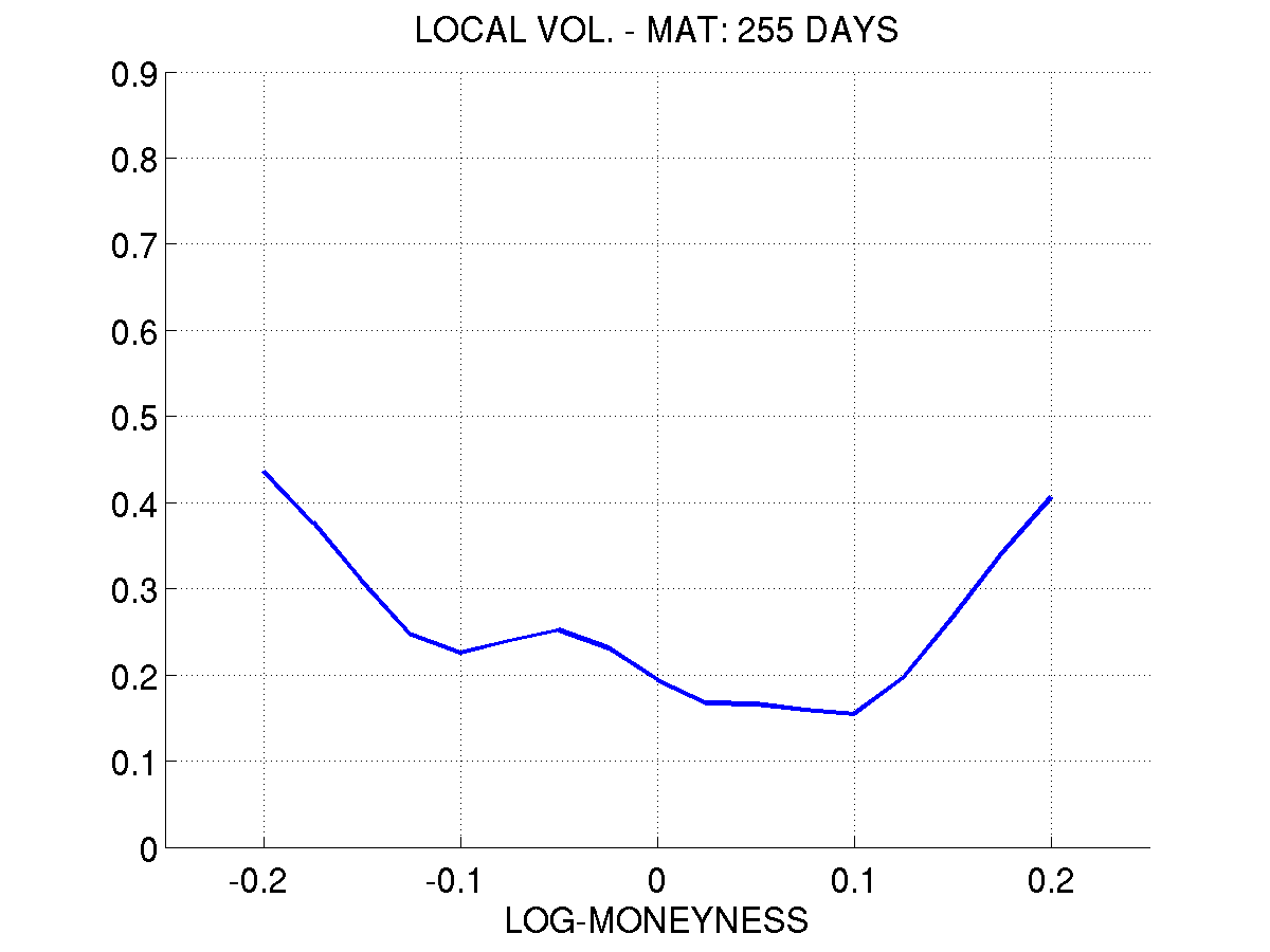
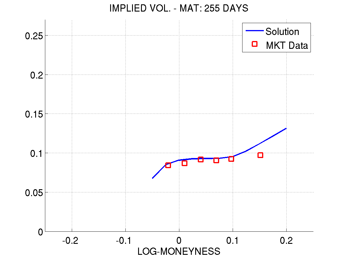
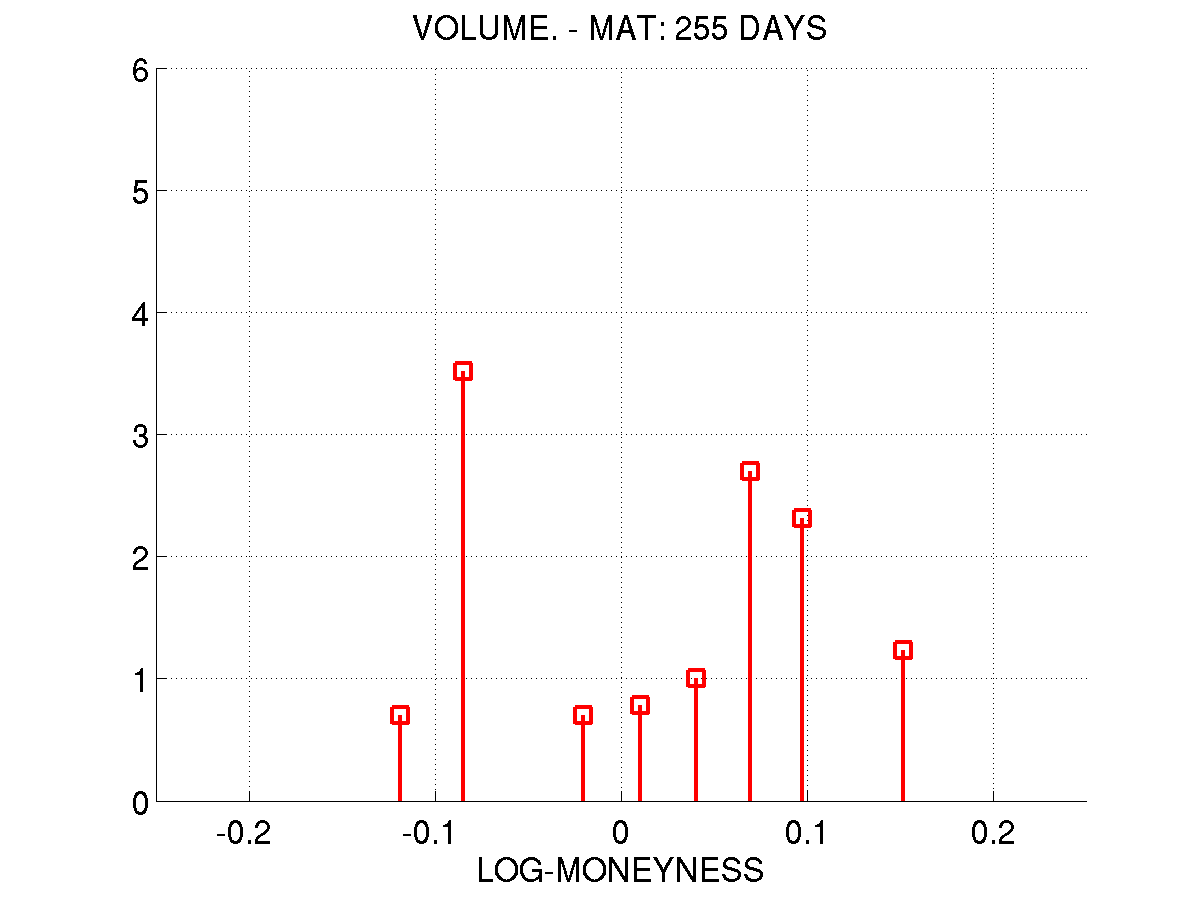
Figure 10: Left: Local volatility reconstructed from S&P500 call option prices traded on 05/09/2013 maturing on 01/18/2014. Center: Implied volatility of market data (squares) and implied volatility of the local volatility of the first figure (continuous line). Right: Volume of the prices used in this reconstruction in a $\log_{10}$ scale.

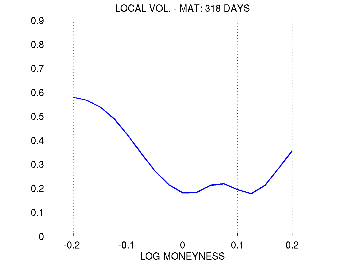
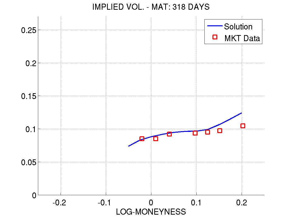
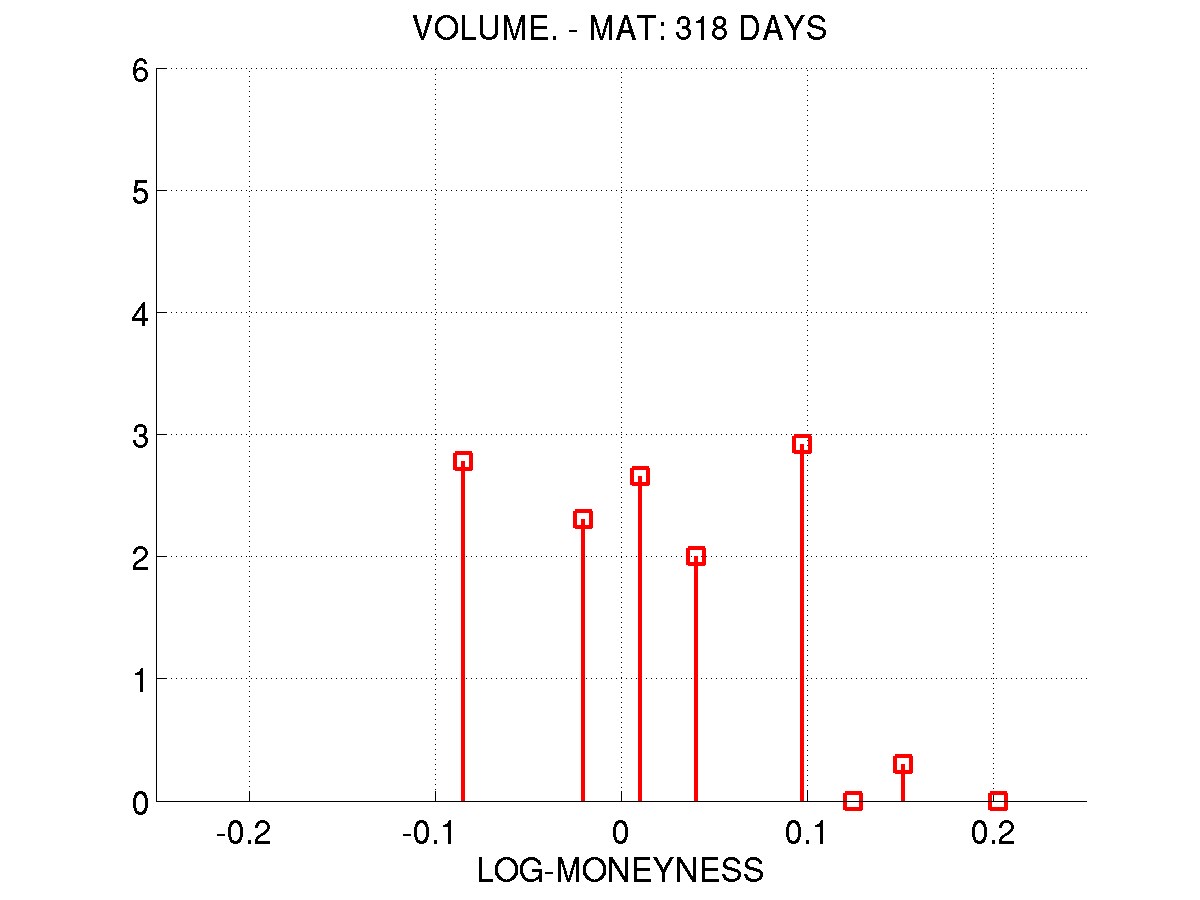
Figure 11: Left: Local volatility reconstructed from S&P500 call option prices traded on 05/09/2013 maturing on 03/22/2014. Center: Implied volatility of market data (squares) and implied volatility of the local volatility of the first figure (continuous line). Right: Volume of the prices used in this reconstruction in a $\log_{10}$ scale.

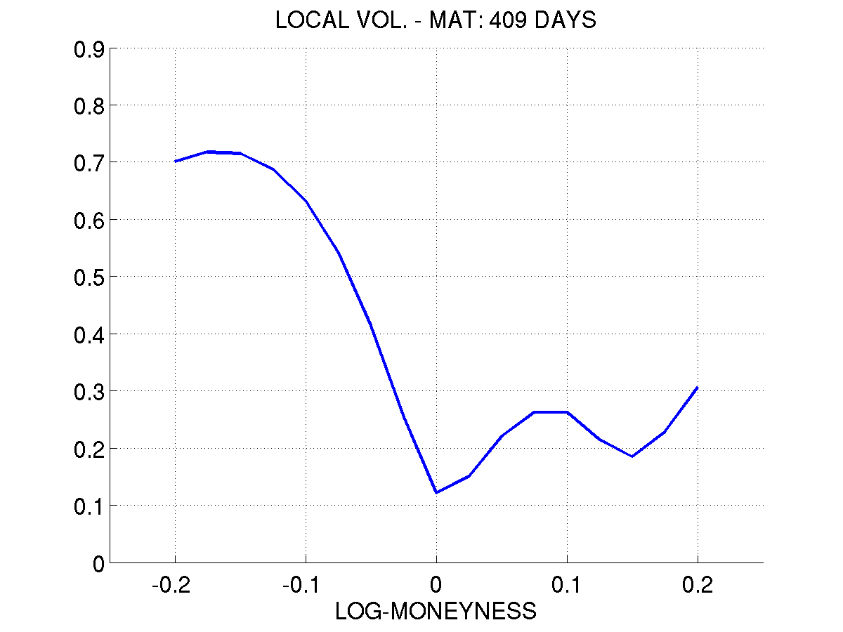
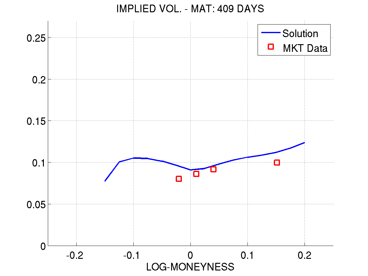
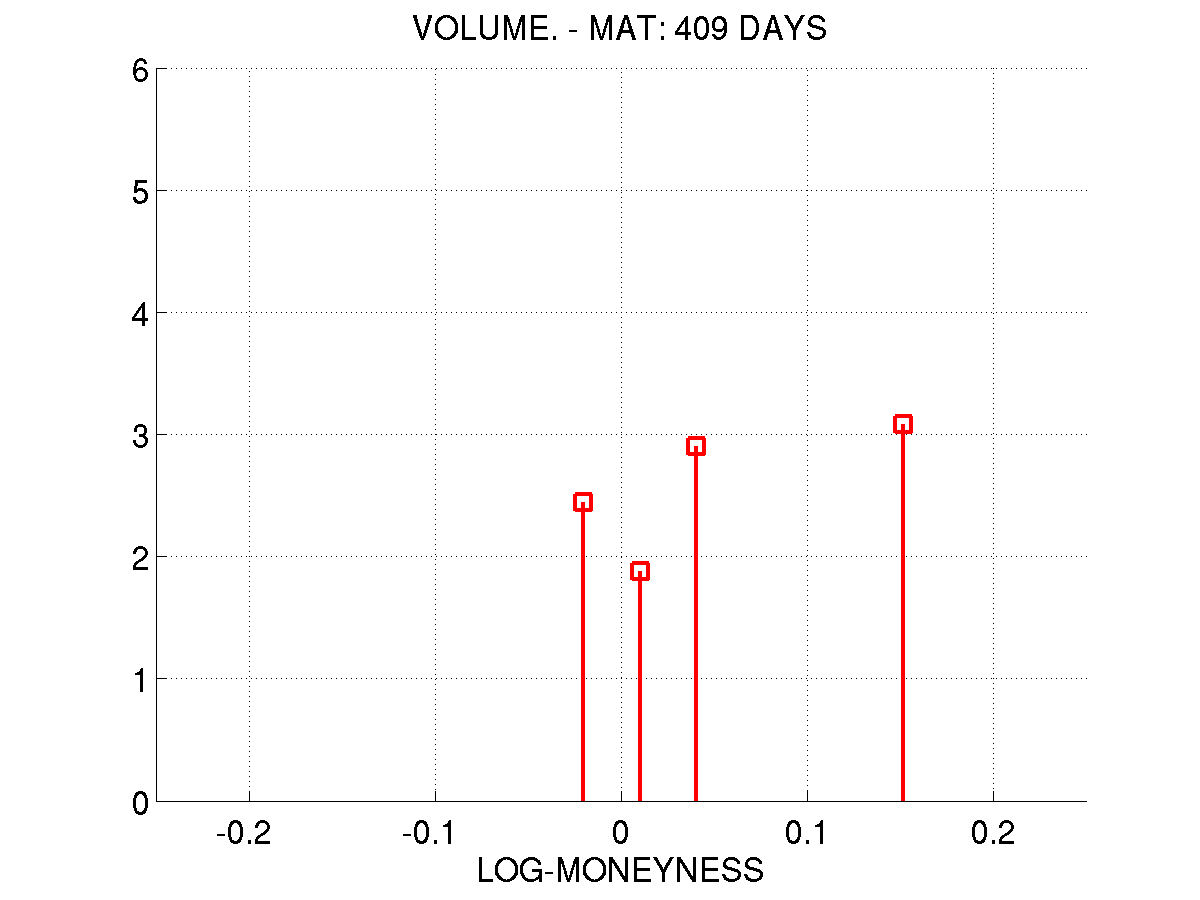
Figure 12: Left: Local volatility reconstructed from S&P500 call option prices traded on 05/09/2013 maturing on 06/21/2014. Center: Implied volatility of market data (squares) and implied volatility of the local volatility of the first figure (continuous line). Right: Volume of the prices used in this reconstruction in a $\log_{10}$ scale.

The left picture in Figures 8, 9, 10, 11 and 12, presents the calibrated local volatility curves from S&P500 call option data for different maturities. Although we have used a piecewise linear basis, the required smoothness was satisfied by the reconstructions. The center picture presents the implied volatility of market data (squares) and implied volatility of the prices related to the local volatility of the left picture (continuous line). Note that these two implied volatility are very close, specially when the trading volume of prices, presented in the right picture, is high, i.e., the prices are more liquid.

Note that, intuitively, more liquid prices are less subject to noise introduced by trading. Then, such numerical results show a strong agreement with our theoretical results of previous sections.

5 Conclusions and Final Remarks

Although our approach emphasizes the discreteness of the data and of the domain where the reconstruction is taking place, it does not rely on a binomial tree approach or a discrete stochastic process. Thus the approach differs substantially from attempts to calibrate the transition probability of the binomial tree of previous works such as [30]

As mentioned in the introduction, one of the novelties of our approach to this subject is that of establishing convergence and convergence rate results of the discrete approximation. Such a result allows us to take into account different levels of uncertainties in the traded prices and convert it into estimates for the choice of the discretization level of the volatility calibration.

In particular, our theoretical and numerical results show that there exists an intrinsic connection between different levels of uncertainty in the data and the corresponding calibrated volatility surface. Furthermore, if the uncertainty level goes to zero, then the calibrated volatility converges to the true volatility. Finally, if we have an upper bound on the financial data uncertainty, then there exists an optimal choice for the discretization level of the volatility surface. Although we do not present a theoretical proof, we proposed a discrepancy principle to determine the optimal discretization level. This claim is illustrated by the results of Section 4.1. The theoretical aspects concerning the implementation of this discrepancy principle are beyond the scope of the present work and shall be discussed in [4].

We also presented reconstructions of the local volatility surface with market data. Using S&P500 data as a validation criteria, we compared the implied volatility obtained from traded data and the prices given by the model. This was compared to the volume information in the validation of results. As expected, the more liquid the traded contracts, the better the results. In other words, the implied volatilities almost coincided for highly traded option strikes and maturities. These results can be found in Section 4.3.

We also applied our technique to Henry Hub natural gas data. In this case, we used the same criteria for validating the results, but we did not have volume information. However, for prices near or at the money, we also had a good match of the implied volatilities of market and model prices. This is justified by the natural higher liquidity of the prices around the at-the-money level. These results can be found in Section 4.2.

Appendix A Properties of the forward operator and ill-posedness of the inverse problem

We now summarize some properties of the operator $F$ that have appeared in the literature [19, 16, 24, 28, 27]. Such properties were used to prove some regularizing aspects of the approximate solutions of the inverse problem under consideration.

Theorem 9.

1. The operator $F\,:\,{\cal D}({F})\subset H^{1+\varepsilon}(D)\longrightarrow W^{1,2}_{2}(D)$ is compact. Moreover, $F$ is weakly (sequentially) continuous and thus weakly closed.

2. Let $D$ be a bounded subset of $\mathbb{R}^{2}$ with Lipschitz boundary. Moreover, let $a_{n}\in\mathcal{D}(F)$ with $a_{n}\rightharpoonup a$ in $L^{2}(D)$. Then $F(a_{n})\rightharpoonup F(a)$ in $L^{2}(D)$.

3. $F$ is differentiable at $a\in{\cal D}({F})$ in the direction $h$ such that $a+h\in{\cal D}({F})$. The derivative $F^{\prime}(a)$ satisfies

   $$-(u^{\prime}\cdot h)_{\tau}+a((u^{\prime}\cdot h)_{yy}-(u^{\prime}\cdot h)_{y})=-h(u_{yy}-u_{y})$$ (34)

   with homogeneous boundary and initial conditions. Also, $F^{\prime}(a)$ is extendable to a bounded linear operator on $H^{1+\varepsilon}(D)$, i.e.,

   $$||F^{\prime}(a)h||_{W^{1,2}_{2}(D)}\leq C||h||_{H^{1+\varepsilon}(D)}.$$ (35)

   Moreover, $F^{\prime}(a)$ satisfies the Lipschitz condition

   $${\left\lVert F^{\prime}(a)-F^{\prime}(a+h)\right\rVert}_{\mathcal{L}(H^{1+\varepsilon}(D);W^{1,2}_{2}(D))}\leq c{\left\lVert h\right\rVert}_{H^{1+\varepsilon}(D)}\,,$$ (36)

   for $a+h\in{\cal D}({F})$.

Proof.

Items (1) and (3) were proved in [19, 24]. Item 2 was proved in [19]. ∎

Remark 3.

An immediate consequence of the compactness and weak closedness of the operator $F$ (see Theorem 9) is the local ill-posedness of the volatility calibration problem. See [19, 24].

The next lemma was already known in [19], however, we present it here for sake of completeness.

Lemma 10.

The Fréchet derivative of the operator $F$,

$$F^{\prime}(a):H^{1+\varepsilon}(D)\longrightarrow W^{1,2}_{2}(D)\,,$$

is injective and compact.

A consequence of Lemma 10 is the fact that $F$ cannot be constant along any affine subspace through $a$ and parallel to $\mathcal{N}(F^{\prime}(a))$. Hence, the tangential cone condition, presented in the theorem below, does not represent a severe assumption in the present context. See the comments in [26, Chapter 11]. The proof of the following theorem can be found in [17, 20].

Theorem 11.

The parameter-to-solution map $F\,:\,{\cal D}({F})\subset H^{1+\varepsilon}(D)\longrightarrow W^{1,2}_{2}(D)$ satisfies the local tangential cone condition, there exists $0<\eta<1/2$ s.t.

$${\left\lVert F(a)-F(\tilde{a})-F^{\prime}(\tilde{a})(a-\tilde{a})\right\rVert}_{W^{1,2}_{2}(D)}\leq\eta{\left\lVert F(a)-F(\tilde{a})\right\rVert}_{W^{1,2}_{2}(D)}\,,$$ (37)

for all $a,\tilde{a}$ in a ball $B_{\rho}(a^{*})\subset\mathcal{D}(F)$ with some $\rho>0$.

In particular, there exists $0<\widetilde{\eta}<1/2$ s.t.

$${\left\lVert F(a)-F(\tilde{a})-F^{\prime}(\tilde{a})(a-\tilde{a})\right\rVert}_{W^{1,2}_{2}(D)}\leq\widetilde{\eta}{\left\lVert a-\tilde{a}\right\rVert}_{H^{1+\varepsilon}(D)}{\left\lVert F(a)-F(\tilde{a})\right\rVert}_{W^{1,2}_{2}(D)}\,,$$ (38)

for all $a,\tilde{a}$ in a ball $B_{\rho}(a^{*})\subset\mathcal{D}(F)$ with some $\rho>0$.

References

- [1] Y. Achdou and O. Pironneau, Computational Methods for Option Pricing, Frontiers in Applied Mathematics, SIAM, 2005.
- [2] R. A. Adams, Sobolev spaces, Academic Press [A subsidiary of Harcourt Brace Jovanovich, Publishers], New York-London, 1975. Pure and Applied Mathematics, Vol. 65.
- [3] V. V. L. Albani, Volatility Calibration in Equity and Commodity Markets by Convex Regularization, PhD thesis, IMPA, 2012.
- [4] V. V. L. Albani, A. De Cezaro, and J. Zubelli, A discrepancy-based choice for domain discretization level and parameter in Tikhonov-type regularization, Working Paper, (2013).
- [5] V. V. L. Albani and J. P. Zubelli, Online Local Volatility Calibration by Convex Regularization with Morozov’s Principle and Convergence Rates, Submitted, (2012).
- [6] M. Avellaneda, The minimum-entropy algorithm and related methods for calibrating asset-pricing model, in Trois applications des mathématiques, vol. 1998 of SMF Journ. Annu., Soc. Math. France, Paris, 1998, pp. 51–86.
- [7] , The minimum-entropy algorithm and related methods for calibrating asset-pricing models, in Proceedings of the International Congress of Mathematicians, Vol. III (Berlin, 1998), no. Extra Vol. III, 1998, pp. 545–563 (electronic).
- [8] , Minimum-relative-entropy calibration of asset-pricing models, International Journal of Theoretical and Applied Finance, 1 (1998), pp. 447–472.
- [9] M. Avellaneda, R. Buff, C. Friedman, N. Grandchamp, L. Kruk, and J. Newman, Weighted Monte Carlo: A new technique for calibrating asset-pricing models. Spigler, Renato (ed.), Applied and industrial mathematics, Venice-2, 1998. Selected papers from the ‘Venice-2/Symposium’, Venice, Italy, June 11-16, 1998. Dordrecht: Kluwer Academic Publishers. 1-31 (2000)., 2000.
- [10] M. Avellaneda, C. Friedman, R. Holmes, and D. Samperi, Calibrating volatility surfaces via relative-entropy minimization., Appl. Math. Finance, 4 (1997), pp. 37–64.
- [11] H. Berestycki, J. Busca, and I. Florent, An inverse parabolic problem arising in finance, Journal of Financial and Quantitative Analysis, 31 (2000), pp. 143–159.
- [12] I. Bouchouev and V. Isakov, The inverse problem of option pricing, Inverse Problems, 13 (1997), pp. L11–L17.
- [13] M. Burger and S. Osher, Convergence rates of convex variational regularization, Inverse Problems, 20 (2004), pp. 1411–1421.
- [14] D. Butnariu and A. N. Iusem, Totally convex functions for fixed points computation and infinite dimensional optimization, vol. 40 of Applied Optimization, Kluwer Academic Publishers, Dordrecht, 2000.
- [15] F.H. Clarke, Optimization and Nonsmooth Analysis, Wiley-Interscience, Vancouver, 1983. 1th edition.
- [16] S. Crépey, Calibration of the local volatility in a generalized Black-Scholes model using Tikhonov regularization, SIAM J. Math. Anal., 34 (2003), pp. 1183–1206 (electronic).
- [17] A. De Cezaro, On a Parabolic Inverse Problem Arising in Quantitative Finance: Convex and Iterative Regularization, in IMPA Thesis, C111 / 2010, IMPA, Rio de Janeiro, 2010, pp. 1–117.
- [18] A. De Cezaro, O. Scherzer, and J.P. Zubelli, A Convex Regularization Framework for Local Volatility Calibration in Derivative Markets: The Connection with Convex Risk Measures and Exponential Families, 6th World Congress of the Bachelier Finance Society, (2010), pp. 1–19.
- [19] A. De Cezaro, O. Scherzer, and J. P. Zubelli, Convex regularization of local volatility models from option prices: convergence analysis and rates, Nonlinear Analysis, 75 (2012), pp. 2398–2415.
- [20] A. De Cezaro and J. P. Zubelli, The tangential cone condition for the iterative calibration of local volatility surfaces, IMA Journal of Applied Mathematics, To Appear.
- [21] E. Derman, I. Kani, and J. Z. Zou, The local volatility surface: Unlocking the information in index option prices, Financial Analysts Journal, 52 (1996), pp. 25–36.
- [22] B. Dupire, Pricing with a smile, Risk, 7 (1994), pp. 18– 20.
- [23] , Private communication, December 2012.
- [24] H. Egger and H. W. Engl, Tikhonov regularization applied to the inverse problem of option pricing: convergence analysis and rates, Inverse Problems, 21 (2005), pp. 1027–1045.
- [25] I. Ekeland and R. Temam, Convex Analysis and Variational Problems, North-Holland, Amsterdam, 1976.
- [26] H. W. Engl, M. Hanke, and A. Neubauer, Regularization of inverse problems, vol. 375 of Mathematics and its Applications, Kluwer Academic Publishers Group, Dordrecht, 1996.
- [27] B. Hofmann, B. Kaltenbacher, C. Pöschl, and O. Scherzer, A convergence rates result for Tikhonov regularization in Banach spaces with non-smooth operators, Inverse Problems, 23 (2007), pp. 987–1010.
- [28] B. Hofmann and R. Krämer, On maximum entropy regularization for a specific inverse problem of option pricing, J. Inverse Ill-Posed Probl., 13 (2005), pp. 41–63.
- [29] J. Jackson, E. Suli, and S. Howison, Computation of deterministic volatility surfaces, J. Comput. Finance, 2 (1998), pp. 5–32.
- [30] J. C. Jackwerth and M. Rubinstein, Recovering stochastic processes from option prices, 1998.
- [31] N. Kahalé, An arbitrage-free interpolation of volatilities, Risk Magazine, (2004), pp. 102–106.
- [32] J. Kaipio and E. Somersalo, Statistical and Computational Inverse Problems, Applied Mathematical Sciences, Springer, 2005.
- [33] R. Lagnado and S. Osher, A Techinque for Calibrating Derivative Security Pricing Models: Numerical Solution of an Inverse Problem, Journal of Computational Finance, 1 (1997), pp. 13–25.
- [34] R. Lee, Implied and local volatilities under stochastic volatility, International Journal of Theoretical and Applied Finance, 4 (2001), pp. 45–89.
- [35] , Implied Volatility: Statics, Dynamics, and Probabilistic Interpretation, Springer, 2005, pp. 241–269.
- [36] V. A. Morozov, Methods for solving incorrectly posed problems, Springer-Verlag, New York, 1984. Translated from the Russian by A. B. Aries, Translation edited by Z. Nashed.
- [37] C. Pöschl, E. Resmerita, and O. Scherzer, Discretization of variational regularization in Banach spaces, Inverse Problems, 26 (2010), pp. 105017, 18.
- [38] E. Resmerita, Regularization of ill-posed problems in Banach spaces: convergence rates, Inverse Problems, 21 (2005), pp. 1303–1314.
- [39] E. Resmerita and R. S. Anderssen, Joint additive Kullback–Leibler residual minimization and regularization for linear inverse problems, 30 (2007), pp. 1527–1544.
- [40] E. Resmerita and O. Scherzer, Error estimates for non-quadratic regularization and the relation to enhancement, Inverse Problems, 22 (2006), pp. 801–814.
- [41] R. T. Rockafellar, Conjugate duality and optimization, Society for Industrial and Applied Mathematics, Philadelphia, Pa., 1974. Lectures given at the Johns Hopkins University, Baltimore, Md., June, 1973, Conference Board of the Mathematical Sciences Regional Conference Series in Applied Mathematics, No. 16.
- [42] D. Samperi, Model calibration using entropy and geometry. 2001.
- [43] O. Scherzer, M. Grasmair, H. Grossauer, M. Haltmeier, and F. Lenzen, Variational Methods in Imaging, vol. 167 of Applied Mathematical Sciences, Springer, New York, 2008.
- [44] P. Wilmott, S. Howison, and J. Dewynne, The mathematics of financial derivatives, Cambridge University Press, Cambridge, 1995. A student introduction.
- [45] C. Zălinescu, Convex analysis in general vector spaces, World Scientific Publishing Co. Inc., River Edge, NJ, 2002.