Independent constraints on local non-Gaussianity from the peculiar velocity and density fields

Abstract

Primordial, non-Gaussian perturbations can generate scale-dependent bias in the galaxy distribution. This in turn will modify correlations between galaxy positions and peculiar velocities at late times, since peculiar velocities reflect the underlying matter distribution, whereas galaxies are a biased tracer of the same. We study this effect, and show that non-Gaussianity can be constrained by comparing the observed peculiar velocity field to a model velocity field reconstructed from the galaxy density field assuming linear bias. The amplitude of the spatial correlations in the residual map obtained after subtracting one velocity field from the other is directly proportional to the strength of the primordial non-Gaussianity. We construct the corresponding likelihood function and use it to constrain the amplitude of the linear flow $\beta$ and the amplitude of local non-Gaussianity $\,f^{\rm{local}}_{\rm{NL}}$. Applying our method to two observational data sets, the Type-Ia supernovae (A1SN) and Spiral Field I-band (SFI++) catalogues, we obtain constraints on the linear flow parameter consistent with the values derived previously assuming Gaussianity. The marginalised 1-D distribution of $\,\left|f^{\rm{local}}_{\rm{NL}}\right|$ does not show strong evidence for non-zero $\,f^{\rm{local}}_{\rm{NL}}$, and we set $95\%$ upper limits $\,\left|f^{\rm{local}}_{\rm{NL}}\right|<51.4$ from A1SN and $\,\left|f^{\rm{local}}_{\rm{NL}}\right|<92.6$ from SFI++. These limits on $\,f^{\rm{local}}_{\rm{NL}}$ are as tight as any set by previous large-scale structure measurements. Our method can be applied to any survey with radial velocities and density field data, and provides an independent check of recent CMB constraints on $\,f^{\rm{local}}_{\rm{NL}}$, extending these to smaller spatial scales.

1 Introduction

In the standard cosmological model, the large-scale structure of the universe has its origin in quantum fluctuations generated during inflation. The simplest single-field, slow-roll inflation model is predicted to generate primordial scalar perturbations that are close to Gaussian and scale-invariant (Bardeen et al., 1986). There exist, however, a large class of alternative models of inflation that can generate significant non-Gaussian components of the gravitational potential (e.g. , 2010). The degree of non-Gaussianity is usually expressed as the amplitude of the bispectrum $B$ normalized by the power spectrum $P$, that is

$$f_{\mathrm{NL}}\equiv\frac{B(k_{1},k_{2},k_{3})}{2\left[P(k_{1})P(k_{2})+P(k_{2})P(k_{3})+P(k_{1})P(k_{3})\right]},$$ (1)

where $k_{1},k_{2}$ and $k_{3}$ are three $k-$space modes. If one assumes that the final evolved potential $\Phi$ is a local function of a primordial Gaussian field $\phi$, then the final potential can be approximated to second order as

$$\Phi=\phi+f_{\mathrm{NL}}^{\mathrm{local}}(\phi^{2}-\langle\phi^{2}\rangle).$$ (2)

This corresponds to the “squeezed” limit ($k_{1}^{2}\ll k_{2}^{2}+k_{3}^{2}$) of the triangle configuration. In this specific case, non-Gaussianity is scale independent, but more generally $f_{\mathrm{NL}}$ as defined in Eq. (1) could depend on scale and on the configuration of the triangle.

The large-scale clustering of galaxies provides an important observational test of primordial non-Gaussianity. Galaxies should trace fluctuations in the underlying matter field to some degree, but may be more or less clustered than the matter distribution as a whole. If, for instance, galaxies form only in the densest peaks of the matter field, which collapse into bound dark matter haloes, these peaks will cluster more strongly than the field on average. In the limit of small amplitude fluctuations, fluctuations in the galaxy distribution $\delta_{\mathrm{g}}$ and fluctuations in the matter distribution $\delta_{\mathrm{m}}$ can be assumed to be proportional and related by a (linear) bias parameter $b$: $\delta_{\mathrm{g}}=b\delta_{\mathrm{m}}$. For peaks in a Gaussian random field, the properties of this halo bias are well understood (Bardeen et al., 1986). In the case of (local) non-Gaussianity, however, 2008 and Matarrese & Verde 2008 have shown that the halo distribution is affected by an additional, scale-dependent bias factor. In particular, a large value of $f_{\mathrm{NL}}^{\mathrm{local}}$ implies that the amplitude of the two-point correlation function is larger on large scales than would be expected in the Gaussian case. A definitive detection of this excess clustering signal could rule out the single-field slow-roll inflation models, and yield insight into the mechanism that drove the inflaton field in the early Universe.

Several studies have used observed clustering to constrain non-Gaussianity. (2011) found $\,f^{\rm{local}}_{\rm{NL}}=48\pm 20$ [$1\sigma$ confidence level (CL)], using radio sources from the NRAO VLA Sky Survey (NVSS), the quasar and MegaZ-LRG (DR7) catalogues of the Sloan Digital Sky Survey (SDSS, York et al. 2000), and the final SDSS II Luminous Red Galaxy (LRG) photometric redshift survey. Nikoloudakis et al. (2013) found $f_{\mathrm{NL}}^{\mathrm{local}}=90\pm 30$ at $1\sigma$ CL using photometric SDSS data , but suggested that this result may be better interpreted as $f_{\mathrm{NL}}^{\mathrm{local}}<120$ at $84\%$ CL, due to the concern over systematics. In addition, (2013) used SDSS-III Baryon Oscillation Spectroscopic Survey (BOSS) data, which were included in the SDSS data release nine (DR9) to constrain the $f_{\mathrm{NL}}^{\mathrm{local}}$ value, and found $-45<f^{\mathrm{local}}_{\mathrm{NL}}<195$ at $2\sigma$ CL, and $P(f^{\mathrm{local}}_{\mathrm{NL}}>0)=91\%$.

Currently, however, the most stringent constraints on non-Gaussianity, at least in a scale-independent form, come from measurements of the bispectrum of the Cosmic Microwave Background (CMB). In 2011, the 7-year Wilkinson Microwave Background Probe (WMAP) data were used to obtain $-10<f_{\mathrm{NL}}^{\mathrm{local}}<74$ at $95\%$ CL (Komatsu et al., 2011). Later, the 9-year WMAP data (, 2013) were used to provide a similar constraint $-3<f_{\mathrm{NL}}^{\mathrm{local}}<77$ at $95\%$ CL. Most recently, Planck released its nominal mission survey results, which constrain local non-Gaussanity to be $f_{\mathrm{NL}}^{\mathrm{local}}=2.7\pm 5.8$ at $68\%$ CL (, 2013). Although these constraints have already placed tight limits on many variant models of inflation, they only probe non-Gaussianity over a limited range of scales and geometries. Thus in principle it remains interesting to develop complementary tests of non-Gaussianity based on large-scale structure. In this paper we introduce a new method for constraining primordial non-Gaussianity by using measurements of the local peculiar velocity field.

In the standard gravitational instability picture, the peculiar velocity field is induced by the gravitational pull of inhomogeneities in the matter distribution, and can be expressed as ${\rm\pi}$ (, 1980)

$$\mathbf{v}_{\mathrm{g}}(\mathbf{r})=\frac{H_{0}f_{0}}{4\pi}\int d^{3}\mathbf{r}^{\prime}\delta_{\mathrm{m}}(\mathbf{r}^{\prime},t_{0})\frac{(\mathbf{r}^{\prime}-\mathbf{r})}{\left|\mathbf{r}^{\prime}-\mathbf{r}\right|^{3}},$$ (3)

where $H_{0}=H(t_{0})$ is the Hubble parameter at the present epoch, $f_{0}$ is the present day growth rate (henceforth we drop the subscript $0$) and $\delta_{\mathrm{m}}$ is the underlying dark matter perturbation, i.e. $\delta_{\mathrm{m}}\equiv(\rho-\overline{\rho})/\overline{\rho}$. Assuming galaxies roughly trace the underlying matter distribution on large scales, then the density contrasts of the two should be related by a linear, deterministic bias factor, $\delta_{\mathrm{g}}=b\delta_{\mathrm{m}}$. On the other hand, if primordial non-Gaussianity exists, the relationship between $\delta_{\mathrm{g}}$ and $\delta_{\mathrm{m}}$ is no longer a single constant bias factor, but depends on scale. This scale-dependent bias may in turn cause a scale-dependence in the relationship between the velocity and density fields. A measurement of this relationship would therefore constrain primordial non-Gaussianity.

Before we move on, we should mention that if $\delta_{\rm g}$ and $\delta_{\rm m}$ are related by a constant bias factor, one can replace the growth rate of density fluctuations $f$ with the dimensionless “linear flow" parameter $\beta\equiv f/b$ (e.g. 2012). The amplitude of the peculiar velocity field scales linearly with $\beta$; its value can be estimated by comparing peculiar velocities derived from distances and redshifts with a model velocity field reconstructed from the density distribution using Eq. (3). The estimated value for the linear flow parameter is $\beta\simeq 0.54$ (, 2012). Many previous studies have performed this “$v$-$v$” analysis, comparing the observed and reconstructed velocity fields; the two match each other fairly well, which constitutes good observational evidence for the gravitational instability paradigm (, 1996, 2001, 2001, 2001, 2002, 2012). In this paper, we want to extend this method to include the contribution from primordial non-Gaussianity, and use state-of-art peculiar velocity field data sets to constrain $f^{\mathrm{local}}_{\mathrm{NL}}$.

This paper is organized as follows. In Sect. 2, we will model the non-Gaussianity, establish its relation to the measured and reconstructed velocity fields, and construct the likelihood function. In Sect. 3, we present the observed and modelled peculiar velocity data, which we will use to constrain the primordial non-Gaussianity. We then present and discuss the results of the likelihood analysis in Sect. 4, and compare the models with and without non-Gaussianity. The conclusions will be presented in the last section.

Throughout the paper, we assume a spatially flat cosmology with Planck parameter values (, 2013), i.e. fractional matter density $\Omega_{\rm m}=0.3183$, fractional baryon density multiplied by Hubble constant squared $\Omega_{\rm b}h^{2}=0.022$, fractional cold dark matter density with Hubble constant squared $\Omega_{\rm c}h^{2}=0.12038$, Hubble constant $h=0.67$ (in unit of $100\,{\rm km}\,{\rm s^{-1}}\,{\rm Mpc^{-1}}$), spectral index of primordial power spectrum $n_{\rm s}=0.962$, and amplitude of fluctuations $\sigma_{8}=0.83$.

2 Method

In this section, we first discuss the physics of the density and velocity fields of galaxies (Sect. 2.1), and then construct a likelihood method to quantify the non-Gaussianity present in the local density field (Sect. 2.2).

2.1 Scale-dependent bias from non-Gaussianity

As shown in both Matarrese et al. (2000) and later in (2008), Matarrese & Verde (2008) and (2009), primordial non-Gaussianity changes the mass function of dark matter haloes, with positive $f^{\mathrm{local}}_{\mathrm{NL}}$ increasing the abundance of high-mass haloes. Non-Gaussianity also changes the bias of the halo distribution relative to the matter distribution, however.

In the Gaussian case, this bias has two components (, 2008): the Lagrangian bias ($b_{\rm L}=b-1$), which reflects the contribution of long-wavelength modes to boosting peaks over the threshold for collapse, and the Eulerian bias, an extra factor of unity which reflects the net excess of matter in over dense regions, or equivalently the motions of primordial peaks at later times. Primordial non-Gaussianity affects the initial conditions (which peaks in the primordial density field become haloes), but not the subsequent gravitational evolution as peaks get advected along with bulk matter flows. Thus the quantity that determines the non-Gaussian bias correction is the Lagrangian bias $b_{\rm L}$, not the Eulerian bias $b$.

The non-Gaussian contribution causes a scale-dependent bias in the power spectrum of dark matter haloes. If one expresses the (Gaussian) dark matter halo bias as a constant factor $b$, the total additional bias is (, 2008; Matarrese & Verde, 2008; , 2013)

$$\Delta b(k)=(b-1)f_{\mathrm{NL}}^{\mathrm{local}}A(k),$$ (4)

where the function $A(k)$ is

$$A(k)=\frac{3\delta_{\rm c}(z)\Omega_{\rm m}h^{2}}{k^{2}T(k)}\left(\frac{H_{0}}{c}\right)^{2}.$$ (5)

Here $k$ is in units of $h\,\text{Mpc}^{-1}$, $T(k)$ is the transfer function, and $\delta_{\rm c}(z)=1.686/D(z)$ is the critical over-density for dark matter haloes to collapse at redshift $z$ from the spherical collapse model, while $D(z)$ is normalized to unity at $z=0$ (, 2013). In our case, since most samples are within $100\,{h^{-1}{\rm Mpc}}$, we take $D(z=0)=1$ in our analysis. We calculate the transfer function and linear matter power spectrum $P_{\mathrm{m}}(k)$ by using the public software package camb (, 2000). We plot the function $A(k)$ in Fig. 1. One can see that the effect of local non-Gaussianity is to increase bias preferentially on large scales. If there is large local non-Gaussianity, it means that there is a correlation between short- and long-wavelength modes, since the geometry of local non-Gaussianity is a triangle with two very long $k$-vectors and one short one ($k_{1}\simeq k_{2}\gg k_{3}$). This means that the locations of massive haloes will be correlated (or anti-correlated) with peaks in the very long wavelength modes of the matter distribution. The function $A(k)$ describes how much enhancement is obtained from this correlation on different scales.

Figure 1: Scale-dependence $A(k)$ of the non-Gaussian bias factor $\Delta b(k)$ (cf. Eq. (5)).

The total bias is a combination of Gaussian linear bias and the additional non-Gaussian bias (Eq. (4)):

$$b_{\mathrm{tot}}=b+\Delta b(k).$$ (6)

Then because $\delta_{\rm g}=b_{\rm{tot}}(k)\delta_{\rm m}$, the galaxy power spectrum $P_{\mathrm{g}}(k)$ is related to the underlying matter power spectrum through

$$P_{\mathrm{g}}(k) = b^{2}_{\mathrm{tot}}(k)P_{\mathrm{m}}(k)$$ (7)

$$= b^{2}P_{\mathrm{m}}(k)+2b\Delta b(k)P_{\mathrm{m}}(k)+\Delta b^{2}(k)P_{\mathrm{m}}(k).$$

The cross-correlation spectrum of density $\delta$ with velocity divergence $\theta=\nabla\cdot\mathbf{v}$ becomes

$$P_{\theta\delta} = \langle(Hf\delta_{\rm m}(k))\delta_{\rm g}(k)\rangle$$ (8)

$$= b_{\mathrm{tot}}(k)HfP_{\rm m}(k).$$

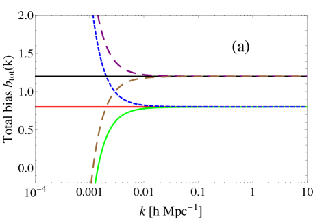
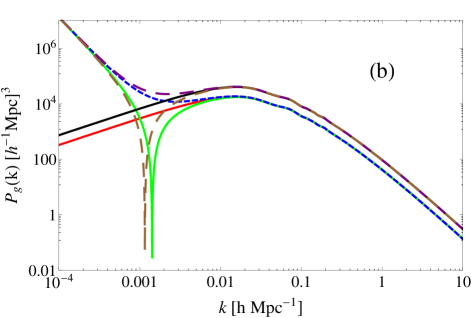
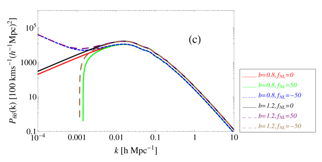
Figure 2: (a): Total bias (Eq. (6)) as a function of $k$. (b): Galaxy power spectrum. (c): Galaxy and velocity divergence cross-correlation power spectrum. The legend for the colour scheme is shown on the right-hand side of panel (c).

In Figs. 2(a)–(c), we plot the total bias and galaxy power spectrum as a function of $k$ over the range $10^{-4}$ to $10h\,\text{Mpc}^{-1}$. In Fig. 2a, comparing to the case of $f^{\mathrm{local}}_{\mathrm{NL}}=0$, one can see that either positive or negative $\,f^{\rm{local}}_{\rm{NL}}$ tends to bias the galaxy power spectrum on very large scales, but whether the bias is positive or negative depends also on the value of $b$. Note that the non-Gaussian correction to the bias [the function $A(k)$ in Fig. 1] can completely dominate the Gaussian bias at large scales. Therefore in Fig. 2, we choose six sets of parameters to represent different values of Eulerian bias $b$ and non-Gaussianity $\,f^{\rm{local}}_{\rm{NL}}$ for different initial conditions of the fluctuations. We describe each of these below.

1. $\,f^{\rm{local}}_{\rm{NL}}=0$ and $b>1$ (black solid lines). The primordial perturbations are Gaussian, and $b>1$ so the objects are more clustered than matter, and as a result they more easily form large-scale overdensities.

2. $\,f^{\rm{local}}_{\rm{NL}}=0$ and $b<1$ (red solid lines). Here the primordial perturbations are Gaussian, but the objects are anti-correlated with respect to the matter fluctuations. The haloes with anti-Lagrangian bias ($b_{\rm L}<0$) are always low mass objects, well below the typical halo mass ($\sim 10^{10}{\rm M}_{\odot}$). Such low-mass haloes only survive today if they have avoided being incorporated into more massive objects, and thus they preferentially avoid high-density regions and therefore they are anti-biased. Such an anti-bias can suppress the strength of the galaxy power spectrum at all scales (red solid line in Fig. 2b).

3. $\,f^{\rm{local}}_{\rm{NL}}>0$ and $b>1$ (purple long-dashed lines). In this case, objects such as galaxies are more clustered than the matter distribution, and small-scale fluctuations in the galaxy distribution are positively correlated with large-scale fluctuations, so that $b_{\rm{tot}}$ at large scales becomes a large positive number. This enhances the galaxy power spectrum ($P_{\rm gg}$) and galaxy-velocity divergence ($P_{\theta\delta}$) power spectrum at large scales.

4. $\,f^{\rm{local}}_{\rm{NL}}>0$ and $b<1$ (green lines). When $b<1$ this means that the primordial haloes and peaks are anti-biased with respect to matter fluctuations. Non-Gaussianity with positive $\,f^{\rm{local}}_{\rm{NL}}$ generates a correlation between the small-scale modes that form haloes and large-scale modes. The second term of Eq. (6) therefore suppresses the clustering of haloes on some certain scales. In addition, one can see that at $k\sim 0.0015\,{h{\rm Mpc}^{-1}}$, the total bias $b_{\rm{tot}}(k)$ (Eq. (6)) vanishes, so that haloes are uncorrelated with matter, producing a nearly-vanishing galaxy power spectrum at this scale (the spike in Fig. 2b).

5. $\,f^{\rm{local}}_{\rm{NL}}<0$ and $b>1$ (brown long-dashed lines). This corresponds to the case where the galaxies formed are related to peaks in the primordial matter fluctuation, but the negative $\,f^{\rm{local}}_{\rm{NL}}$ means that those small peaks are associated with large-scale troughs of matter fluctuations. The total bias is therefor suppressed at large scales.

6. $\,f^{\rm{local}}_{\rm{NL}}<0$ and $b<1$ (blue dashed lines). Here the galaxy overdensities are anti-correlated with the matter fluctuations, so the galaxies form in the troughs of the primordial density field. However since $\,f^{\rm{local}}_{\rm{NL}}<0$, these troughs are associated with the large-scale peaks of the galaxy distribution. Therefore, the fact that galaxy small-scale overdensities and large-scale modes are both anti-correlated with small-scale density fluctuations mean that they are positively correlated with each other. Therefore one obtains a positive total bias factor between $\delta_{\rm g}$ and $\delta_{\rm m}$.

No matter which subcases that the initial conditions fall into, on the very large scales ($k\lesssim 10^{-4}\,{h{\rm Mpc}^{-1}}$) the galaxy power spectra with $\,f^{\rm{local}}_{\rm{NL}}\neq 0$ all converge with each other. This indicates that at very large scales, the primordial non-Gaussianity induced correlation always dominates the clustering properties of galaxies.

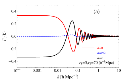
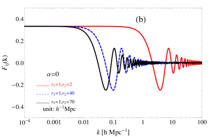
Figure 3: Angular dependence function $F_{ij}(k)$ for different choices of the length of vectors $r_{i}=r_{1},r_{j}=r_{2}$ and their angular separation $\alpha$. In panel (a), we fix the lengths of two vectors and plot $F_{ij}(k)$ with three values of the separation angle $\alpha$, while in panel (b), we fix $\alpha=0$ and vary the length of the second vector $r_{2}$.

2.2 Constraining $\,f^{\rm{local}}_{\rm{NL}}$ with peculiar velocities

Now let us calculate the peculiar velocity field and reconstructed density field in the framework of non-Gaussian initial fluctuations. The real-space 3D velocity field (Eq. (3)) can also be expressed in Fourier space as

$$\mathbf{v}(\mathbf{r})=\frac{iH_{0}f}{(2\pi)^{3}}\int{\rm d}^{3}\mathbf{k}\delta_{\rm m}(\mathbf{k})\frac{\mathbf{k}}{k^{2}}\exp\left(i\mathbf{k\cdot r}\right).$$ (9)

Now we substitute $\delta_{\rm g}(\mathbf{k})=b_{\rm{tot}}(k)\delta_{\rm m}(\mathbf{k})$ into the above equation, and after some arrangement, we have

$$\mathbf{v}(\mathbf{r}) = \frac{iH_{0}f}{(2\pi)^{3}}\int{\rm d}^{3}\mathbf{k}\frac{\delta_{\rm g}(\mathbf{k})}{b_{\rm{tot}}(k)}\frac{\mathbf{k}}{k^{2}}\exp\left(i\mathbf{k\cdot r}\right)$$ (10)

$$= \frac{iH_{0}f}{(2\pi)^{3}}\int{\rm d}^{3}\mathbf{k}\left(\frac{1}{b}+\frac{1}{b_{\rm{tot}}(k)}-\frac{1}{b}\right)\delta_{\rm g}(\mathbf{k})\frac{\mathbf{k}}{k^{2}}\exp\left(i\mathbf{k}\cdot\mathbf{r}\right)$$

$$= \frac{iH_{0}f}{(2\pi)^{3}}\int{\rm d}^{3}\mathbf{k}\frac{1}{b}\delta_{\rm g}(\mathbf{k})\frac{\mathbf{k}}{k^{2}}\exp\left(i\mathbf{k}\cdot\mathbf{r}\right)$$

$$+ \frac{iH_{0}f}{(2\pi)^{3}}\int{\rm d}^{3}\mathbf{k}\left(\frac{b-b_{\rm{tot}}(k)}{b\cdot b_{\rm{tot}}(k)}\right)\delta_{\rm g}(\mathbf{k})\frac{\mathbf{k}}{k^{2}}\exp\left(i\mathbf{k}\cdot\mathbf{r}\right).$$

Absorbing the linear reconstruction $\beta=f/b$ into the first term, performing a Fourier transform, and substituting Eq. (6) into the second term, we obtain

$$\mathbf{v}(\mathbf{r}) = \frac{H_{0}\beta}{4\pi}\int{\rm d}^{3}\mathbf{r^{\prime}}\delta_{\rm g}(\mathbf{r^{\prime}})\frac{\mathbf{r^{\prime}}-\mathbf{r}}{|\mathbf{r^{\prime}}-\mathbf{r}|^{3}}$$ (11)

$$- \frac{iH_{0}(f/b)}{(2\pi)^{3}}\int{\rm d}^{3}\mathbf{k}(\Delta b(k))\delta_{\rm m}(\mathbf{k})\frac{\mathbf{k}}{k^{2}}\exp\left(i\mathbf{k}\cdot\mathbf{r}\right),$$

in which we can see that the primordial non-Gaussianity produces an additional term in the velocity field.

Now we consider the meaning of the two terms in Eq. (11). The first term is the linear peculiar velocity field reconstruction from observed galaxy distribution, which in the following section, will be represented by the IRAS 1.2 Jy and PSC$z$ (Point Source Catalogue redshift) samples (, 1995, 2000). The second part is the additional 3D velocity term coming from the non-Gaussian structures which arise from the presence of local non-Gaussianity. This will appear as a residual velocity field $v^{\rm res}=v^{\rm mea}-\beta v^{\rm rec}$ if we subtract the linearly reconstructed field from the observed one. Since we can only measure the line-of-sight velocity of distant galaxies, we need to project Eq. (11) on to the radial direction. We define the projected left-hand-side of Eq. (11) as $v^{\rm{mea}}_{i}=\mathbf{v}(\mathbf{r})\cdot\hat{r}_{i}$ for the $i\rm{th}$ object, since this represents the measured line-of-sight velocity. We then define the projected first term in the right-hand-side as $\beta v^{\rm{rec}}_{i}$ for the reconstructed velocity for the $i\rm{th}$ object, where $v^{\rm{rec}}_{i}$ is the reconstructed velocity with normalization $\beta=1$. Now we can move the first term from the right hand side to the left and calculate the covariance matrix for the residual velocities $v^{\rm res}_{i},v^{\rm res}_{j}$:

$$C_{ij} = \left\langle v^{\rm res}_{i}v^{\rm res}_{j}\right\rangle$$

$$= \left\langle(v^{\rm{mea}}_{i}-\beta v^{\rm{rec}}_{i})(v^{\rm{mea}}_{j}-\beta v^{\rm{rec}}_{j})\right\rangle$$

$$= \frac{H_{0}^{2}(f/b)^{2}}{(2\pi)^{6}}\int{\rm d}^{3}\mathbf{k_{1}}{\rm d}^{3}\mathbf{k_{2}}(\Delta b(k))^{2}\langle\delta_{\rm m}(\mathbf{k}_{1})\delta_{\rm m}(\mathbf{k}_{2})\rangle$$

$$\times \frac{(\mathbf{k_{1}}\cdot\hat{r}_{i})(\mathbf{k_{2}}\cdot\hat{r}_{j})}{(k_{1}k_{2})^{2}}\exp\left(i(\mathbf{k_{1}}\cdot\mathbf{r}_{i}-\mathbf{k_{2}}\cdot\mathbf{r}_{j})\right)$$

$$\ +\ \delta_{ij}(\sigma^{2}_{i}+\sigma^{2}_{\ast}),$$

where $\sigma_{i}$ is the measurement error of the $i\rm{th}$ object, $\delta_{ij}$ is the kronecker delta symbol, and $\sigma_{\ast}$ is the intrinsic small-scale velocity dispersion. Substituting the ensemble average of the matter density contrast $\langle\delta_{\rm m}(\mathbf{k}_{1})\delta_{\rm m}(\mathbf{k}_{2})\rangle=(2\pi)^{3}\delta^{3}(\mathbf{k}_{1}-\mathbf{k}_{2})P_{\rm{m}}(k)$, and Eq. (4), we obtain

$$C_{ij}=\frac{H^{2}_{0}}{2\pi^{2}}\left(f-\beta\right)^{2}I_{ij}+\delta_{ij}(\sigma^{2}_{i}+\sigma^{2}_{\ast}),$$ (13)

where

$$I_{ij}=\left(f^{\rm{local}}_{\rm{NL}}\right)^{2}\int{\rm d}kP_{\rm{m}}(k)A^{2}(k)F_{ij}(k),$$ (14)

and $F_{ij}(k)$ is the integral of angle over the full-sky

$$F_{ij}(k)=\frac{1}{4\pi}\int{\rm d}\Omega_{k}(\hat{k}\cdot\hat{r}_{i})(\hat{k}\cdot\hat{r}_{j})\exp\left(i\mathbf{k}\cdot\left(\mathbf{r}_{i}-\mathbf{r}_{j}\right)\right),$$ (15)

which can be calculated analytically. In the appendix of (2011) it is shown that

$$F_{ij}(k)=\frac{1}{3}\cos\alpha(j_{0}(k\tilde{r})-2j_{2}(k\tilde{r}))+\frac{1}{\tilde{r}^{2}}j_{2}(k\tilde{r})r_{i}r_{j}\sin^{2}\alpha,$$ (16)

with

$$\tilde{r}=\left|\mathbf{r}_{i}-\mathbf{r}_{j}\right|=\left[r^{2}_{i}+r^{2}_{j}-2r_{i}r_{j}\cos(\alpha)\right]^{1/2}.$$ (17)

From Eqs. (16) and (17), one can see that $F_{ij}(k)$ only depends on three values: the length of vectors $\mathbf{r}_{i}$ and $\mathbf{r}_{j}$ (i.e. $r_{i}$ and $r_{j}$), and their separation angle $\alpha$ ($\cos(\alpha)=\hat{r}_{i}\cdot\hat{r}_{j}$). In Fig. 3, we plot the function $F_{ij}(k)$ by taking different sets of parameter values. In Fig. 3a, we fix the length of the two vectors $r_{1}=5\,{h^{-1}{\rm Mpc}}$ and $r_{2}=70\,{h^{-1}{\rm Mpc}}$, and vary the separation angle $\alpha$. One can see that different $\alpha$ values determine the amplitude of the function $F_{ij}$. As $\alpha$ increases from $0$ to $\pi$, the amplitude of $F_{ij}$ in the low-$k$ plateau flips from positive to negative, and its value is close to zero if $\alpha\rightarrow\pi/2$. However, no matter what $\alpha$ value is taken, $F_{ij}(k)$ oscillates very quickly and converges to zero at $k>0.02\,{h{\rm Mpc}^{-1}}$. In Fig. 3b, we fix $\alpha=0$ and plot $F_{ij}(k)$ by varying the length of the second vector $r_{2}$. One can see that if $r_{1}$ is close to $r_{2}$, the function starts to dominate at larger $k$ (basically $k>1\,{h{\rm Mpc}^{-1}}$); on the other hand, if $r_{1}$ and $r_{2}$ differ by a large value, then the function will only be constant for $k<0.02\,{h{\rm Mpc}^{-1}}$ and will oscillate quickly and converge to zero at large $k$ values.

The shape of the function $F_{ij}(k)$ is important because the covariance between velocities of different objects on the sky (Eqs. (13) and (14)) is the matter power spectrum filtered by the functions $F_{ij}(k)$ and $A^{2}(k)$. $F_{ij}(k)$ oscillates and converges to zero very quickly at large $k$, and $A(k)$ also decays very rapidly when the value of $k$ becomes larger (Fig. 1). Therefore, the total covariance $I_{ij}$ is sensitive to the large-scale behaviour of the filtered function $P_{\rm{m}}(k)$, i.e. $I_{ij}$ is sensitive to scales $k<0.02\,{h{\rm Mpc}^{-1}}$ and does not depend on the small-scale modes of the matter power spectrum very much. In this sense, the covariance matrix method proposed above is valid for the detection of non-Gaussianity because as we see in Fig. 2, the major signature of primordial non-Gaussianity is in the very large-scale galaxy density power spectrum.

Although most of the effect of non-Gaussianity is on large scales, our filter function retains some sensitivity to smaller scales. Fig. 3a, for instance, shows that the correlation between two galaxies is larger for small values of the separation angle $\alpha$. In Fig. 3b, we see that for small separation angle and small difference in the radial distance ($r_{1}\sim r_{2}$), the correlation signal can extend down to $k=1$–$2\,{h{\rm Mpc}^{-1}}$, although non-linear corrections and errors in distance and velocity will become important on these small scales. In comparison, the CMB probes non-Gaussianity to $\ell=1500$, which corresponds to structures with scales $0.0264$ Mpc at the last scattering surface, evolving to $\sim 30$ Mpc at the present day. This CMB sensitive scale corresponds to $k\sim 0.03\,{h{\rm Mpc}^{-1}}$, while we can go down to $1\,{h{\rm Mpc}^{-1}}$, so we can extend these constraints by an order of magnitude in $k$, albeit with poor sensitivity.

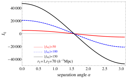
Figure 4: Velocity condition quantity $I_{ij}$ (Eq. (14)) as a function of separation angle $\alpha$ when choosing different $\,f^{\rm{local}}_{\rm{NL}}$ parameters. One can see that if the separation angle between two objects is less (greater) than $\pi/2$, the correlation is positive (negative), and the amplitude of the correlation is proportional to the magnitude of the local non-Gaussianity.

We also plot (in Fig. 4) the quantity $I_{ij}$ as a function of separation angle $\alpha$, while varying the $\,f^{\rm{local}}_{\rm{NL}}$ parameter. One can see that if $\alpha<\pi/2$, the two separated objects tend to be correlated, while if $\alpha>\pi/2$, they tend to be anti-correlated. The amplitude of the correlation is proportional to the magnitude of local non-Gaussianity $\,f^{\rm{local}}_{\rm{NL}}$. In addition, the shape of the correlation function $I_{ij}$, as a function of $\alpha$, is very similar to a cosine function. This important feature will allow us to obtain robust estimates of the $\,f^{\rm{local}}_{\rm{NL}}$ value, for the following reason. In the case of ordinary spiral galaxies, the dispersion $\sigma_{\ast}$ accounts for the small-scale non-linear motions which are believed to have a variance around $300\,{\rm km}\,{\rm s}^{-1}$ (, 2007). We will assume this value in the following likelihood analysis procedure. However, we can see that the assumption of this particular value does not make much difference in estimating the absolute magnitude of $\,f^{\rm{local}}_{\rm{NL}}$. This is because, as seen in Fig. 4, $I_{ij}$ is only sensitive to the angular separation of the two objects in different directions, so this modulation function is close to a first order polynomial function $P_{1}(\alpha)=\cos(\alpha)$, which is orthogonal to the “monopole” moments of the correlation ($\sigma_{\ast}$). Therefore, it is the spatial correlation between different directions of the objects that really constrains $\,f^{\rm{local}}_{\rm{NL}}$.

Therefore returning to Eq. (13), one can see that if we subtract the density-reconstructed $v^{\rm{rec}}_{i}$ from the observed peculiar velocity field, covariance in the residual field will consist of three parts: the primordial non-Gaussianity induced cross-correlation between different velocities, which is proportional to $I_{ij}$; the measurement error of the line-of-sight velocity $\sigma_{ij}$; and the intrinsic small-scale velocity dispersion $\sigma_{*}$. If there is no non-Gaussianity, i.e. $\,f^{\rm{local}}_{\rm{NL}}=0$, then $I_{ij}=0$ and the first term of the right-hand-side of Eq. (13) vanishes, so there is no correlation between different directions of the residual velocity field. This corresponds to the Gaussian case, where the residual field is absolutely randomly distributed across the whole sky. The covariance matrix is then diagonal and is determined only by the measurement errors and the small-scale velocity and intrinsic dispersion terms.

On the other hand, if the residual map shows correlations in velocity from one region of the sky to another, it may indicate the presence of primordial non-Gaussianity at some level. Thus the covariance of the residual map will provide a quantitative measure of the effects of local non-Gaussianity. To constrain $f_{NL}^{\rm local}$, we can formulate a likelihood function

$$L(\beta,\,f^{\rm{local}}_{\rm{NL}})=\frac{1}{\sqrt{\det(C)}}\times$$

$$\exp\bigg{\{}-\frac{1}{2}\left(v^{\rm{mea}}_{i}-\beta v^{\rm{rec}}_{i}\right)C_{ij}^{-1}\left(v^{\rm{mea}}_{j}-\beta v^{\rm{rec}}_{j}\right)\bigg{\}},$$ (18)

where $\,f^{\rm{local}}_{\rm{NL}}$ is contained in $C$ and $\beta$ is contained in both $C$ and the data vector. In the following, we will apply this likelihood function to a peculiar velocity field data set to constrain the values of $\beta$ and $\,f^{\rm{local}}_{\rm{NL}}$.

3 Data

From the derivation above we see that in order to quantify the primordial non-Guassianity present in the primordial density field, we need to subtract from the observed peculiar velocity field a model reconstructed from the density field assuming linear bias, and measure the variance of the residual velocities in different directions. In this section, we first introduce the observed peculiar velocity field data sets and then the model velocity field data set.

3.1 The observed peculiar velocity field

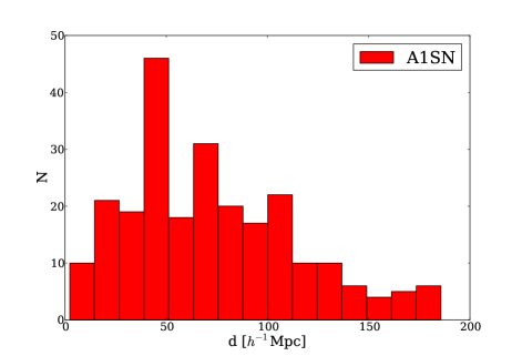
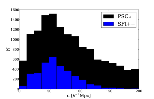
Figure 5: Distance distributions for the A1SN (left-hand panel), SFI++ and PSC$z$ (right-hand panel) catalogues.

The observed peculiar velocity field data set is of course the most important ingredient of the data analysis. In this work we focus on two different catalogues, A1SN and SFI++. There are several reasons for choosing these two catalogues. First, they are high-quality and recently assembled peculiar velocity data sets that deeply sample our local volume. Secondly, they both have full-sky coverage, which allows us to constrain the correlation of objects in different directions. Thirdly, the distance estimators for the two data sets are completely independent of each other, therefore minimizing the chance of systematic error, and providing us a self-consistent check of the results.

The A1SN catalogue is known as the “First Amendment” supernovae sample, and consists of $245$ Type-Ia supernovae compiled by (2012). The data set is merged from three different Type-Ia supernovae data sets: (1) $106$ samples from (2007) and (2009); (2) another $113$ objects collected by (2009); and (3) the $28$ objects observed by the “Carnegie Supernovae project” (, 2010). Supernovae observations use the luminosity-distance relation as the “standard candle”, so the distance error is typically $7$ per cent, much smaller than for the other galaxy Fundamental Plane or Tully–Fisher-relation-determined distances. The characteristic depth of the whole catalogue is $58\,{h^{-1}{\rm Mpc}}$.

The Spiral Field I-band (SFI++) catalogue is the largest and densest survey of peculiar velocities available to date (, 2007), and consists of $3456$ spiral galaxies with peculiar velocities derived from the Tully–Fisher relation (, 1977). Most of the galaxies are in the field (2675) or in groups (726) (, 2009). The distribution of the galaxies across the sky is remarkably homogeneous, as shown in fig. 1 of (2010) and (2012). Since distances in the catalogue are derived by using the Tully–Fisher relation, the typical distance errors are around $23$ per cent. The characteristic depth of the SFI++ catalogue is around $40$-$50\,{h^{-1}{\rm Mpc}}$, as is shown in the right-hand panel of Fig. 5.

In the left-hand panel of Fig. 5, we show the distribution of distances in the A1SN sample, while in the right-hand panel we plot the distributions for the PSC$z$ and SFI++ samples. By comparing these three samples, we can see that the distribution of A1SN and SFI++ is very close to a scaled down version of the PSC$z$ sample, so that the shape of the distance distribution is quite self-similar in each case. The three data sets also have similar depths. This is another reason we choose the A1SN and SFI++ data sets to compare with the PSC$z$ model velocities.

In general, these samples become sparser and errors increase at large distances. If we include the “outliers” in the range of $70$-$130\,{h^{-1}{\rm Mpc}}$, for instance, the scatter among $\beta$ values increases, indicating there may be systematic errors in either the measured or model velocity field (, 2012). To be conservative, we exclude galaxies outside $70\,{h^{-1}{\rm Mpc}}$ and just use the samples within this range. With this cut, we retain $126$ A1SN samples, and $2044$ SFI++ samples for the final data set.

As a last step, since we perform the likelihood analysis in the Local Group frame, we transform the velocities provided in the CMB frame by subtracting the line-of-sight component of the Local Group velocity determined from the CMB dipole, i.e. $v=611\,{\rm km}\,{\rm s}^{-1}$ towards $(l,b)=(269^{\circ},+28^{\circ})$ (see Scott & Smoot 2010).

3.2 Model density and velocity fields

In order to search for the effects of non-Gaussianity, we also need a model velocity field. In this paper we use the model velocity field obtained (, 1999) from the IRAS PSC$z$ catalogue (, 2000). The spatial distribution of PSC$z$ galaxies is fairly homogeneous across the sky [cf. 2012, fig. 1, panels (a) and (b)], which is ideal for studying the cross-correlation with galaxies in different directions.

PSC$z$ redshift catalogues were used to trace the underlying mass distribution within $300\,{h^{-1}{\rm Mpc}}$, with the assumption of linear and deterministic bias (, 2004, 2012). The reconstructed velocity field was obtained by performing the integration of the first term of right hand side of Eq. (11) by using the iterative technique of (1991). The iteration procedure includes only objects within $130\,{h^{-1}{\rm Mpc}}$, since at larger distances the samples are very sparse and do not strongly affect peculiar velocities within the $70\,{h^{-1}{\rm Mpc}}$ volume. In this way, we obtain the final reconstructed peculiar velocities for $8995$ PSC$z$ galaxies within $130\,{h^{-1}{\rm Mpc}}$ that were not collapsed into galaxy clusters (, 2012).

The distribution of distances in the PSC$z$ catalogue is plotted in the right-hand panel of Fig. 5. Note that we only use the $d<70\,{h^{-1}{\rm Mpc}}$ galaxies for the likelihood analysis, but use the samples out to $130\,{h^{-1}{\rm Mpc}}$ to model the gravitational pull of the distant structures.

Since the PSC$z$ predicted velocities outnumber the observed peculiar velocities, we need to interpolate the predicted velocities at the position of the galaxies in the peculiar velocity data sets (, 2012). We perform such “smoothing” by applying a Gaussian kernel of the same radius $R_{j}\simeq 5\,{h^{-1}{\rm Mpc}}$ to the predicted velocity field, i.e. we calculate

$$\mathbf{v}_{\rm{smo}}(\mathbf{r}_{i})=\frac{\sum_{j=1}^{N}\mathbf{v}_{\rm{rec}}(\mathbf{r}_{j})\exp\left(-\frac{(\mathbf{r}_{j}-\mathbf{r}_{i})^{2}}{2R_{j}^{2}}\right)}{\sum_{j=1}^{N}\exp\left(-\frac{(\mathbf{r}_{j}-\mathbf{r}_{i})^{2}}{2R_{j}^{2}}\right)},$$ (19)

where we sum over $N$ PSC$z$ galaxies at position $\mathbf{r}_{j}$ to interpolate to the position of galaxy ($\mathbf{r}_{i}$) in the peculiar velocity catalogue. We then project the smoothed velocities on to the line-of-sight direction to compare with the observed velocity.

As we pointed out in our previous work (, 2012), the typical random errors of the model velocity field are $130\,{\rm km}\,{\rm s}^{-1}$ (, 1999), much smaller than the observed velocities. In our earlier $v$–$v$ comparison, we initially gnored this random error, but eventually found a relatively large value of a “hyper-parameter” which indicates the amplitude of underestimated errors. In this work, we group all of these random errors and unaccounted systematics into one parameter, $\sigma_{\ast}$ (see Eqs. (LABEL:eq:variance1) and (13)). Since the random errors of the reconstructed velocities are around $130\,{\rm km}\,{\rm s}^{-1}$, the thermal velocities are typically $\sim 250\,{\rm km}\,{\rm s}^{-1}$ (, 2007), and there may be other systematics unaccounted for, we set the parameter $\sigma_{\ast}=300\,{\rm km}\,{\rm s}^{-1}$. Changing this parameter to be larger or smaller value does not strongly affect the constraints on $\,f^{\rm{local}}_{\rm{NL}}$, because these come mainly from the “dipole” modulation of the covariance matrix while the $\sigma_{\ast}$ is a monopole term.

4 Results

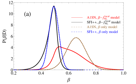
Figure 6: Left – marginalized distribution of the $\beta$ parameter with and without the correlation term in the covariance matrix (Eqs. (LABEL:eq:variance1) and (13)). Right – marginalized distribution of the $\,\left|f^{\rm{local}}_{\rm{NL}}\right|$ parameter for the model including non-Gaussianity-induced spatial correlations.

Data set	Model	$\beta$ value	$\,\left|f^{\rm{local}}_{\rm{NL}}\right|$ value	$-\log L_{\rm{min}}$
A1SN	$\beta$-$\,f^{\rm{local}}_{\rm{NL}}$	$0.53^{+0.15}_{-0.04}$	$0.0\pm 25.7$	$681.7$
	$\beta$-only	$0.65^{+0.07}_{-0.06}$		$681.7$
SFI++	$\beta$-$\,f^{\rm{local}}_{\rm{NL}}$	$0.49^{+0.03}_{-0.05}$	$26.6\pm 33.0$	$14159.1$
	$\beta$-only	$0.49^{+0.04}_{-0.03}$		$14159.1$

Table 1: The results of constraints from A1SN and SFI++ data sets. All of the errors quoted are $1\sigma$ CL.

By substituting the observed line-of-sight velocities $v^{\rm{mea}}_{i}$ and reconstructed velocities $v^{\rm{rec}}_{i}$ ($i=1,...N$) into Eq. (18), we can obtain the joint likelihood of $\beta$ and $\,\left|f^{\rm{local}}_{\rm{NL}}\right|$. Note that in Eq. (14), the covariance matrix is proportional to $\,\left|f^{\rm{local}}_{\rm{NL}}\right|$, so the likelihood can only determine the absolute magnitude of $\,f^{\rm{local}}_{\rm{NL}}$. In Fig. 6, we plot the probability distribution of $\beta$ (panel a) and $\,\left|f^{\rm{local}}_{\rm{NL}}\right|$ (panel b) by using the A1SN and SFI++ catalogues. We also list our results in Table 1.

In Fig. 6a, we plot the probability distribution of $\beta$. In this figure, we combine the results both from the model which includes correlations between different directions in the residual velocities (Eqs. (LABEL:eq:variance1) and (13)) and the model just with measurement errors and small-scale and intrinsic dispersion [i.e. only with second term in Eqs. (LABEL:eq:variance1) and (13)]. In Fig. 6 and the following, we refer to these as the $\beta$-$\,f^{\rm{local}}_{\rm{NL}}$ and the $\beta$-only models, respectively. One can see that for the SFI++ data set, the best-fitting value of $\beta$ is $0.49$, close to the value we obtained from the “hyper-parameter” method (, 2012). By neglecting the correlation term, the peak of the distribution does not change, but the width of the distribution is reduced. In this sense, the additive covariance term from primordial non-Gaussianity (Eqs. (LABEL:eq:variance1) and (13)) broaden the distribution of the $\beta$ parameter, without shifting the best-fitting value very much.

The same is true of the A1SN data set, except that the peak of the distribution shifts a little towards a slightly lower $\beta$ value. For both the data sets, the $\beta$ values found are consistent with each other, and are also consistent with the values found in (2012), indicating that the growth of structure rate ($f\sigma_{8}$) is consistent with the prediction of the $\Lambda$-Cold-Dark-Matter ($\Lambda$CDM) model.

In Fig. 6b, we plot the marginalized distribution of $\,f^{\rm{local}}_{\rm{NL}}$, using the likelihood function (Eq. (18)). One can see that both data sets prefer the $\,\left|f^{\rm{local}}_{\rm{NL}}\right|$ value to be very small, consistent with zero within $1\sigma$ CL. A1SN data prefers the $\,\left|f^{\rm{local}}_{\rm{NL}}\right|<27$ at $68\%$ CL, and SFI++ data suggest $\,\left|f^{\rm{local}}_{\rm{NL}}\right|<59.6$ at $68\%$ CL. These two upper bounds are the strongest upper limits we can obtain from current measurements of the local peculiar velocity field. Overall, our constraints on $\,f^{\rm{local}}_{\rm{NL}}$ are tighter than any derived previously from large-scale structure measurements (e.g. 2011, $\,f^{\rm{local}}_{\rm{NL}}=48\pm 20$ at $1\sigma$ CL.; Nikoloudakis et al. 2013, $\,f^{\rm{local}}_{\rm{NL}}=90\pm 30$ at $1\sigma$ CL.; and 2013, $\,f^{\rm{local}}_{\rm{NL}}<195$ at $1\sigma$ CL.). This constraint is still considerably weaker than the recent result from (2013) ($\,f^{\rm{local}}_{\rm{NL}}=2.7\pm 5.8$), but it does cover a slightly different range of scales, and in general provides an independent confirmation at low redshift. The peculiar velocity constraint could also be improved with more data from a future velocity survey.

If there really was a primordial non-Gaussian correlation between objects in different directions of the sky, the negative log-likelihood function of the full covariance matrix would be much lower than the diagonal one alone. This is not the case, however. In Table 1, we list the minimum value of $-\log L$ for both of the likelihoods, with and without spatial correlations. One can see that the two likelihood methods give the same value of $-\log L$, suggesting that the two models provide the same goodness of fit. However, since the full-covariance matrix has one more parameter than the $\beta$-only model, the current observational data from the peculiar velocity field and model velocity field do not support strong evidence of large $\,f^{\rm{local}}_{\rm{NL}}$.

5 Conclusion

Primordial cosmological perturbations are usually assumed to have Gaussian statistics, as expected in single-field inflation models. Many variants on single-field inflation predict deviations from Gaussianity, however, and there have been some tentative claims of non-Gaussianity from previous observations of large-scale structure (, 2011; Nikoloudakis et al., 2013; , 2013). Here we have shown that measurements of local peculiar velocities and density fields set strong constraints on departures from Gaussian initial conditions down to scales 10 times smaller than those probed by the CMB.

The peculiar velocity field of galaxies traces the underlying matter distribution directly, whereas the galaxy density distribution may have a scale-dependent bias with respect to the matter distribution if the initial conditions are (locally) non-Gaussian. The peculiar velocity field can be decomposed into two terms, the velocity field reconstructed assuming linear bias (i.e. the usual Gaussian term) and, a second, residual velocity field. For Gaussian initial conditions, the residual velocity field should be random, without any large-scale spatial correlations. If $\,f^{\rm{local}}_{\rm{NL}}$ is non-zero, however, scale-dependent bias in the galaxy distribution will induce large-scale spatial correlations in the residual velocity field. We construct a likelihood function to quantify the variance of angular correlations in the residual map, and thereby constrain $\,f^{\rm{local}}_{\rm{NL}}$.

Applying our likelihood function to the currently available deep, full-sky surveys of Type-Ia supernovae (A1SN) and spiral galaxies with Tully–Fisher determined distances (SFI++), we find that models with and without local non-Gaussianity give consistent constraints on $\beta$, constraints which are also consistent with our previous work (, 2012). This also confirms that the linear growth rate at the present time is consistent with the predictions for the $\Lambda$CDM model with WMAP and Planck determined cosmological parameters.

More importantly, we can also constrain the amplitude of local non-Gaussianity by comparing the log-likelihood for the models with and without an $\,f^{\rm{local}}_{\rm{NL}}$ term. This analysis provides an upper bound of $\,\left|f^{\rm{local}}_{\rm{NL}}\right|\leq 25.7$ (A1SN), and $\,\left|f^{\rm{local}}_{\rm{NL}}\right|\leq 59.6$ (SFI++) at $1\sigma$ CL. These limits are as tight as any set by previous large-scale structure studies. We find that models with or without non-Gaussianity provide the same “goodness” of fit, indicating that adding the spatial correlation parameter does not improve the fit to the residual velocity field.

Although we do not find any signature of primordial non-Gaussianity, our physical and statistical model is an independent constraint on the primordial initial conditions, complementary to the CMB measurements. This method is applicable to any data set with peculiar velocities and an overlapping estimate of the density. Since Planck has published a full-sky Sunyaev–Zeldovich (SZ) catalogue, for instance, this could be used to derive a full-sky peculiar velocity field for galaxy clusters and compared with large-scale maps of the galaxy distribution, refining the constraints presented here. In addition, if the bulk motion and density distribution of large-scale neutral hydrogen gas can be observed from future 21cm surveys (such as ), our method can also be applied to investigate non-Gaussianity in a higher redshift regime and therefore deeper cosmic volume.

References

- Bardeen et al. (1986) Bardeen, J. M., Bond, J. R., Kaiser, N., & Szalay, A. S. 1986, ApJ, 304, 15
- (2) Bennett C.L. et al., 2013, ApJS, 208, 20
- (3) Branchini E., et al., 1999, MNRAS, 308, 1
- (4) Branchini E., 2001, MNRAS, 326, 1191
- (5) Dalal, N., Doré, O., Huterer, D., & Shirokov, A. 2008, Phys. Rev. D, 77, 123514
- (6) Davis M., Nusser A.; Willick J. A., 1996, ApJ, 473, 22
- (7) Folatelli G. et al., 2010, AJ, 139, 120
- (8) Feldman H. A., Frieman J. A., Fry J. N., Scoccimarro R., 2001, Phys. Rev. Lett., 86, 1434
- (9) Feldman H., Watkins R., Hudson M. J., 2010, MNRAS, 407, 2328
- (10) Fisher K., Huchra J., Strauss M., Davis M., Yahil A., Schlegel D., 1995, ApJ, 100, 69
- (11) Hicken M. et al., 2009, ApJ, 700, 1097
- (12) Jha S., Riess A. G., Kirshner R. P., 2007, ApJ, 659, 122
- Komatsu et al. (2011) Komatsu E. et al. 2011, ApJS, 192, 18
- (14) Lewis A., Challinor A., & Lasenby A., 2000, ApJ, 538, 473
- (15) Ma Y.Z., Gordon C., & Feldman H., 2011, Phys. Rev. D 83, 103002.
- (16) Ma Y.Z., Branchini E., & Scott D., 2012, MNRAS, 425, 2880
- Matarrese et al. (2000) Matarrese, S., Verde, L., & Jimenez, R. 2000, ApJL, 541, 10
- Matarrese & Verde (2008) Matarrese, S., & Verde, L. 2008, ApJL, 677, L77
- Nikoloudakis et al. (2013) Nikoloudakis, N., Shanks, T., & Sawangwit, U. 2013, MNRAS, 429, 2032
- (20) Peebles P. J. E., The Large-Scale Structure of the Universe, Princeton Univ. Press (1980).
- (21) Planck 2013 results XVI, arXiv: 1303.5076 [astro-ph.CO].
- (22) Planck 2013 results XXIV, arXiv: 1303.5084 [astro-ph.CO].
- (23) Radburn-Smith D.J., Lucey J.R., Hudon M.J., 2004, MNRAS, 355, 1378
- (24) Ross A. et al., 2013, MNRAS, 428, 1116
- (25) Saunders W., et al., 2000, MNRAS, 317, 55
- (26) Scoccimarro R., Feldman H. A., Fry J. N., Frieman J. A., 2001, ApJ, 546, 652
- Scott & Smoot (2010) Scott D., Smoot G., Rev. Part. Phys. 2010, (arXiv: 1005.0555)
- (28) Square Kilometre Array: http://www.skatelescope.org
- (29) Springob C. M., Masters K. L., Haynes M. P., Giovanelli R., Marinoni C., 2007, ApJS, 172, 599
- (30) Tully R. B., & Fisher J. R., 1977 A&A, 54, 661
- (31) Turnbull S. J., Hudson M. J., Feldman H. A., Hicken M., Kirshner R. P., Watkins R., 2012, MNRAS, 420, 447
- (32) Verde L. et al., 2002, MNRAS, 335, 432
- (33) Wands D., & Slosar A., 2009, Phys. Rev. D, 79, 123507
- (34) Wands D., 2010, CQG, 27, 124002
- (35) Wang L., ApJ submitted (arXiv: 0705.0368)
- (36) Watkins R., Feldman H. A., Hudson M. J., 2009, MNRAS, 392, 743
- (37) Xia J. Q., Baccigalupi C., Matarrese S., Verde L., & Viel M., 2011, JCAP, 08, 033
- (38) Yahil A., Strauss M.A., Davis M., Huchra J.P., 1991, ApJ, 372, 380
- York et al. (2000) York, D.G., et al. 2000, AJ, 120, 1579