New Prospects for Higgs Compositeness in $h\to Z\gamma$

Aleksandr Azatov, Roberto Contino, Andrea Di Iura, Jamison Galloway 

Dipartimento di Fisica, Università di Roma “La Sapienza”
and INFN Sezione di Roma, I-00185 Rome, Italy

We discuss novel effects in the phenomenology of a light Higgs boson within the context of composite models. We show that large modifications may arise in the decay of a composite Nambu-Goldstone boson Higgs to a photon and a $Z$ boson, $h\to Z\gamma$. These can be generated by the exchange of massive composite states of a strong sector that breaks a left-right symmetry, which we show to be the sole symmetry structure responsible for governing the size of these new effects in the absence of Goldstone-breaking interactions. In this paper we consider corrections to the decay $h\to Z\gamma$ obtained either by integrating out vectors at tree level, or by integrating out vector-like fermions at loop level. In each case, the pertinent operators that are generated are parametrically enhanced relative to other interactions that arise at loop level in the Standard Model such as $h\to gg$ and $h\to\gamma\gamma$. Thus we emphasize that the effects of interest here provide a unique possibility to probe the dynamics underlying electroweak symmetry breaking, and do not depend on any contrivance stemming from carefully chosen spectra. The effects we discuss naturally lead to concerns of compatibility with precision electroweak measurements, and we show with relevant computations that these corrections can be kept well under control in our general parameter space.

1 Introduction

The LHC phase of data taking at 8 TeV is over and a large collection of experimental results on the Higgs boson has been derived. Although data still have to be fully analyzed, a clear picture seems to be emerging: the properties of the newly discovered particle closely resemble those of the Standard Model (SM) Higgs boson. Overall, the quantitative agreement between its measured couplings and the SM predictions is at the $20-30\%$ level [1, 2]. This strongly suggests that the new particle is indeed part of an $SU(2)_{L}$ doublet $H$, and that the scale of New Physics (NP) must be somewhat higher than the electroweak scale. From this perspective it is important to ask which observables or processes are most sensitive to NP effects and where we may be likely to see deviations from the SM pattern in the future.

It is well known that Higgs processes occurring at loop level in the SM, such as the decays $h\to\gamma\gamma$ and $h\to Z\gamma$, and the gluon-fusion production $gg\to h$, are particularly sensitive probes of weakly-coupled extensions of the SM. This is typically not true, however, in theories with a light Higgs where the electroweak symmetry breaking (EWSB) dynamics is strong. If the Higgs is a composite Nambu-Goldstone (NG) boson of a new strongly-interacting sector, parametrically large shifts are expected in the tree-level couplings, while $hgg$ and $h\gamma\gamma$ contact interactions violate the Higgs shift symmetry and are thus suppressed. On the other hand, a similar symmetry suppression does not hold for a $hZ\gamma$ contact interaction.

To make this point more quantitative, contributions to the $gg$, $\gamma\gamma$ and $\gamma Z$ decay rates induced by the exchange of new particles with mass much larger than the electroweak scale can be conveniently parametrized by local operators. For a Higgs doublet, the leading NP effects are parametrized by dimension-6 operators. A complete characterization of the Higgs effective Lagrangian at the dimension-6 level has been performed in previous studies [3, 4, 5]; see Ref. [6] for a recent review. In the basis of the Strongly Interacting Light Higgs (SILH) of Ref. [7], the CP-conserving operators relevant for the $gg$, $\gamma\gamma$ and $Z\gamma$ rates are: 

$$\begin{split}O_{g}&=\frac{g_{S}^{2}}{m_{W}^{2}}H^{\dagger}HG_{\mu\nu}^{a}G^{a\,\mu\nu},\\[5.69046pt] O_{\gamma}&=\frac{g^{\prime\,2}}{m_{W}^{2}}H^{\dagger}HB_{\mu\nu}B^{\mu\nu},\end{split}\qquad\begin{split}O_{HW}&=\frac{ig}{m_{W}^{2}}\,(D^{\mu}H)^{\dagger}\sigma^{i}(D^{\nu}H)W_{\mu\nu}^{i}\\[5.69046pt] O_{HB}&=\frac{ig^{\prime}}{m_{W}^{2}}\,(D^{\mu}H)^{\dagger}(D^{\nu}H)B_{\mu\nu}\,.\end{split}$$ (1.1)

The operators $O_{g}$ and $O_{\gamma}$ contribute respectively to the $gg$ and $\gamma\gamma$ rates, while $Z\gamma$ gets a contribution from both $O_{\gamma}$ and the linear combination $O_{HW}-O_{HB}$. The additional operators

$$O_{W}=\frac{ig}{2m_{W}^{2}}D^{\nu}W_{\mu\nu}^{i}(H^{\dagger}\sigma^{i}{\overleftrightarrow{D^{\mu}}}H)\,,\qquad O_{B}=\frac{ig^{\prime}}{2m_{W}^{2}}\partial^{\nu}B_{\mu\nu}(H^{\dagger}{\overleftrightarrow{D^{\mu}}}H)$$ (1.2)

do not mediate $h\to Z\gamma$ for on-shell photons, but their sum contributes to the $S$ parameter [8]. By working in unitary gauge and focussing on terms with one Higgs boson, the operators of Eq. (1.1) are rewritten as

$${\cal L}=\frac{c_{gg}}{2}\,G^{a}_{\mu\nu}G^{a\,\mu\nu}\frac{h}{v}+\frac{c_{\gamma\gamma}}{2}\,\gamma_{\mu\nu}\gamma^{\mu\nu}\frac{h}{v}+c_{Z\gamma}\,Z_{\mu\nu}\gamma^{\mu\nu}\frac{h}{v}\,,$$ (1.3)

where (by $\bar{c}_{i}$ we denote the coefficient of the operator $O_{i}$ of the SILH Lagrangian) [6]

$$\begin{gathered}c_{gg}=8(\alpha_{s}/\alpha_{2})\,\bar{c}_{g}\,,\quad c_{\gamma\gamma}=8\sin^{2}\!\theta_{W}\,\bar{c}_{\gamma}\,,\\[5.69046pt] c_{Z\gamma}=-\tan\theta_{W}\left[(\bar{c}_{HW}-\bar{c}_{HB})+8\sin^{2}\!\theta_{W}\,\bar{c}_{\gamma}\right]\,,\end{gathered}$$ (1.4)

and $\alpha_{2}=\sqrt{2}G_{F}m_{W}^{2}/\pi$. The expression of the partial decay width to $Z\gamma$, including the SM contribution and the correction from Eq. (1.3) is given in Appendix A.

Let us perform a naive estimate of the size of the effects mediated by the operators of Eq. (1.1). By simple dimensional analysis, the Wilson coefficients $\bar{c}_{i}$ scale as $1/M^{2}$, where $M$ is the characteristic NP scale. Their contribution to the Higgs decay rates is thus suppressed by a factor $\sim(m_{W}^{2}/M^{2})$, where $m_{W}\approx m_{h}$ is the energy scale of the process. If the operators $O_{i}$ are generated by the tree-level exchange of new particles with unsuppressed non-minimal couplings to photons and gluons, one naively expects a correction

$$\frac{\Delta\Gamma_{tree}}{\Gamma_{SM}}\approx\frac{m_{W}^{2}}{M^{2}}\,\frac{16\pi^{2}}{g^{2}}\,.$$ (1.5)

Unsuppressed non-minimal couplings can arise if the new heavy states are bound states of some new strong dynamics, see for example the recent discussion of Ref. [9]. On the other hand, in weakly-coupled UV completions of the SM as well as in some strongly-coupled constructions such as Holographic Higgs models, the massive states have suppressed higher-derivative couplings. In this case the operators $O_{i}$ are generated only at the cost of a loop factor ($g_{*}^{2}/16\pi^{2}$) [7], where $g_{*}$ denotes the coupling strength of the Higgs boson to the new states:

$$\frac{\Delta\Gamma_{loop}}{\Gamma_{SM}}\approx\frac{m_{W}^{2}}{M^{2}}\,\frac{g_{*}^{2}}{g^{2}}\sim\frac{v^{2}}{f^{2}}\,.$$ (1.6)

In the last identity we have defined $1/f\equiv g_{*}/M$. Large corrections are thus possible in strongly-coupled theories, where the Higgs boson is a composite of the new dynamics and $1\ll g_{*}<4\pi$. However, a composite Higgs is naturally light only if it is a NG boson of a spontaneously broken symmetry ${\cal G}\to{\cal H}$ of the strong sector. In this case the scale $f$ must be identified with the associated decay constant, and shifts of order $(v/f)^{2}$ are expected in the tree-level Higgs couplings to SM vector bosons and fermions from the Higgs non-linear $\sigma$-model Lagrangian. At the same time, exact invariance under ${\cal G}/{\cal H}$ transformations, which include a Higgs shift symmetry $H^{i}\to H^{i}+\zeta^{i}$, forbids the operators $O_{g}$ and $O_{\gamma}$. For the latter to be generated the shift symmetry must be broken by some weak coupling $g_{\not G}$, so that the naive estimate of $\bar{c}_{g}$, $\bar{c}_{\gamma}$, and hence their contribution to the decay rates to $gg$ and $\gamma\gamma$, is further suppressed by an extra factor $(g_{\not G}^{2}/g_{*}^{2})$. Conversely, the operators $O_{HW}$ and $O_{HB}$ are invariant under the Higgs shift symmetry, and the naive estimate (1.6) holds for the $h\to Z\gamma$ rate. It follows that for a composite NG Higgs the largest NP effects are expected to arise from shifts to the tree-level Higgs couplings and from the contact $hZ\gamma$ interaction [7]. From this perspective, a precise measurement of the $Z\gamma$ rate is of crucial importance.

It is the purpose of this paper to quantitatively study the $h\to Z\gamma$ decay rate in the context of composite Higgs models. As implied by the discussion above, the leading effects are captured by neglecting the explicit breaking of the Goldstone symmetry due to weak couplings of the elementary fields to the composite sector. We thus work in this limit in the following as it simplifies the calculations, and concentrate on the contributions of pure composite states within minimal $SO(5)/SO(4)$ theories. The next Section contains a brief discussion on the effective operator basis for $SO(5)/SO(4)$ theories and the role played by the $P_{LR}$ parity for the $h\to Z\gamma$ decay. In Section 3 we compute the effective $hZ\gamma$ vertex generated by the tree-level exchange of spin-1 resonances and by the 1-loop exchange of composite fermions. As a byproduct of our $hZ\gamma$ calculation we derive in Section 4 the correction to the $S$ parameter from loops of pure composite fermions. We report our numerical results and discuss them in Section 5. Useful formulas are collected in Appendices A-D, while Appendix E contains a discussion of different formalisms commonly adopted to describe fermionic resonances. Finally, in Appendix F we describe how the calculation of the 1-loop contribution to $h\to Z\gamma$ from heavy fermions can be performed in full generality in the basis of mass eigenstates, without resorting to the approximation made in the main text.

2 Effective Lagrangian for $SO(5)/SO(4)$ composite Higgs models and the role of $P_{LR}$

The effective Lagrangian for $SO(5)/SO(4)$ composite Higgs theories was discussed in Ref. [10], where a complete list of four-derivative operators was given in the formalism of Callan, Coleman, Wess, and Zumino (CCWZ) [11]. Here we closely follow the notation of Ref. [10], although we adopt a different operator basis which is more transparently matched onto the SILH basis of Ref. [7]. At $O(p^{4})$ in the derivative expansion there are seven independent CP-conserving operators 

$${\cal L} =\frac{f^{2}}{4}\text{Tr}\!\left[d_{\mu}d^{\mu}\right]+\sum_{i}c_{i}O_{i}$$ (2.2)

$$\begin{split}O_{1}&=\text{Tr}\!\left[d_{\mu}d^{\mu}\right]^{2}\\[2.84544pt] O_{2}&=\text{Tr}\!\left[d_{\mu}d_{\nu}\right]\text{Tr}\left[d^{\mu}d^{\nu}\right]\\[2.84544pt] O_{3}^{\pm}&=\text{Tr}\!\left[(E^{L}_{\mu\nu})^{2}\pm(E^{R}_{\mu\nu})^{2}\right]\\[2.84544pt] O_{4}^{\pm}&=\text{Tr}\!\left[\left(E^{L}_{\mu\nu}\pm E^{R}_{\mu\nu}\right)i[d^{\mu},d^{\nu}]\right]\\[2.84544pt] O_{5}&=\sum_{a_{L}=1}^{3}\text{Tr}\!\left(T^{a_{L}}[d_{\mu},d_{\nu}]\right)^{2}-\sum_{a_{R}=1}^{3}\text{Tr}\left(T^{a_{R}}[d_{\mu},d_{\nu}]\right)^{2}\,,\end{split}$$ (2.3)

where $d_{\mu}(\pi)=d_{\mu}^{\hat{a}}(\pi)T^{\hat{a}}$, $E^{L}_{\mu}(\pi)=E_{\mu}^{a_{L}}(\pi)T^{a_{L}}$, $E^{R}_{\mu}(\pi)=E_{\mu}^{a_{R}}(\pi)T^{a_{R}}$ are the CCWZ covariant functions—transforming respectively as an adjoint and gauge fields of $SO(4)$—of the NG field $\pi(x)=\pi^{\hat{a}}(x)T^{\hat{a}}$. Explicitly,

$$-iU^{\dagger}(\pi)D_{\mu}U(\pi)=d_{\mu}+E_{\mu}^{L}+E_{\mu}^{R}\,,$$ (2.4)

where $U(\pi)=\exp(i\sqrt{2}\,\pi(x)/f)$. The field strength $E_{\mu\nu}^{L,R}$ is constructed from a commutator of covariant derivatives $\nabla_{\mu}=\partial_{\mu}+i(E_{\mu}^{L}+E_{\mu}^{R})$; see Ref. [10] for further details. Here $T^{a_{L}}$, $T^{a_{R}}$ are the generators of the unbroken $SO(4)\sim SU(2)_{R}\times SU(2)_{R}$, while those of $SO(5)/SO(4)$ are denoted as $T^{\hat{a}}$. The SM electroweak vector bosons weakly gauge an $SU(2)_{L}\times U(1)_{Y}$ subgroup of $SO(5)\times U(1)_{X}$, where the $U(1)_{X}$ does not participate in the dynamical breaking, but is needed to correctly reproduce the hypercharges of the SM fermions. It is convenient to define the tree-level vacuum such that the electroweak group is fully contained in the unbroken $SO(4)\times U(1)_{X}$, with $Y=T^{3R}+T^{X}$. The true vacuum will in general be misaligned with this direction by an angle $\theta$ due to the radiatively induced potential of the NG bosons.

The operators in Eq. (2.3) have been conveniently defined to be even or odd under a parity $P_{LR}$ which exchanges the $SU(2)_{L}$ and $SU(2)_{R}$ comprising the unbroken $SO(4)$. Under $P_{LR}$ the NG bosons transform as $\pi^{\hat{a}}(x)\to-\eta^{\hat{a}}\pi^{\hat{a}}(x)$, with $\eta^{\hat{a}}=\{1,1,1,-1\}$, which implies $d_{\mu}^{\hat{a}}\to-\eta^{\hat{a}}d_{\mu}^{\hat{a}}$, $E^{L}_{\mu}\leftrightarrow E^{R}_{\mu}$ [10]. Ordinary parity is thus the product $P=P_{0}\cdot P_{LR}$, where $P_{0}\,$$:(t,\vec{x})\to(t,-\vec{x})$ is the usual spatial inversion. Under $P_{LR}$, the operators $O_{1,2}$ and $O^{+}_{3,4}$ are even, whereas $O^{-}_{3,4}$ and $O_{5}$ are odd. Expanding in the number of NG fields it is easy to match the operators of Eq. (2.3) with the dimension-6 operators of the SILH Lagrangian by noticing that

$$\begin{split}d_{\mu}&\sim D_{\mu}H+\dots\\ E_{\mu\nu}&\sim A_{\mu\nu}+\frac{1}{f^{2}}\left[D_{\mu}\!\left(H^{\dagger}i{\overleftrightarrow{D_{\nu}}}H\right)-(\mu\leftrightarrow\nu)\right]+\dots\end{split}$$ (2.5)

where the gauge fields entering into the field strength $A_{\mu\nu}$ and the covariant derivative $D_{\mu}$ are those of $SU(2)_{L}\times U(1)_{Y}$. From Eq. (2.5) one can see that $O_{3}^{\pm}$ and $O_{4}^{\pm}$ correspond respectively to $O_{W}\pm O_{B}$ and $O_{HW}\pm O_{HB}$. The leading terms in the expansion of $O_{1}$, $O_{2}$, and $O_{5}$ are instead of dimension 8, meaning that these operators do not have a counterpart in the SILH Lagrangian of Ref. [7]. The exact relations and the connection between our basis and that of Ref. [10] are reported in Appendix B. Notice that there is no operator in Eq. (2.3) corresponding to $O_{\gamma}$ and $O_{g}$, since the latter explicitly break the $SO(5)$ global symmetry. It then follows that the only (CP-conserving) operator which gives a $hZ\gamma$ contact coupling is $O_{4}^{-}$:

$$c_{Z\gamma}=g^{2}\sin^{2}\!\theta\,c_{4}^{-}\,.$$ (2.6)

Notice also that only $O_{3}^{+}$ contributes to the $S$ parameter:

$$S=-32\pi\sin^{2}\!\theta\,c_{3}^{+}\,.$$ (2.7)

It is not an accident that the $hZ\gamma$ coupling follows from a $P_{LR}$-odd operator. Since the abelian $U(1)_{X}$ subgroup factorizes with respect to the non-linearly realized $SO(5)$, the photon and $Z$ fields enter into the operators of Eq. (2.3) only through the weak gauging of the $U(1)_{L}\times U(1)_{R}$ subgroup. By formally assigning the transformation rules $W_{\mu}^{3}\leftrightarrow B_{\mu}$, $g\leftrightarrow g^{\prime}$, the $P_{LR}$ symmetry is exact even after turning on the neutral gauge fields. By the above rules, the $Z$ field is odd while the photon and the Higgs boson are even under $P_{LR}$, so that the decay $h\to Z\gamma$ can be mediated only by an odd operator. By the same argument, $S$ is an even quantity under $LR$ exchange (it is proportional to the coefficients of the unitary-gauge operator $W_{\mu\nu}^{3}B^{\mu\nu}$), and it is consistently induced by the $P_{LR}$-even operator $O_{3}^{+}$.

It is interesting to notice that in the limit of unbroken $SO(5)$ symmetry the RG running of $c_{4}^{-}$, as well as that of the coefficient of any $O(p^{4})$ odd operator, vanishes due to the $P_{LR}$ parity. While the effective operators are generated at some high-energy scale $M$ by the exchange of massive states, the Wilson coefficients appearing in the expressions of low-energy observables, like in Eq. (2.6) for the $Z\gamma$ decay rate, must be evaluated at the typical scale of the process, $\mu\ll M$. The running of the Wilson coefficients from $M$ down to $\mu$ originates from 1-loop logarithmically divergent diagrams constructed with $O(p^{2})$ vertices,

$$c_{i}(\mu)=c_{i}(M)+\frac{b_{i}}{16\pi^{2}}\log\frac{M}{\mu}\,,$$ (2.8)

where $b_{i}$ are $O(1)$ numbers. Since however $P_{LR}$ is an accidental symmetry of the $O(p^{2})$ Lagrangian [10], it follows that there cannot be any running from loops of NG bosons in the case of $P_{LR}$-odd operators, i.e. $b_{i}=0$.  An RG evolution is in general induced by loops of transverse vector bosons,  since the weak gauging explicitly breaks $P_{LR}$ at the $O(p^{2})$ level. This is however a subleading electroweak effect which we neglect for simplicity in this paper. One naively expects $c_{i}(M)\sim 1/16\pi^{2}$ for operators generated at the scale $M$ with an extra loop suppression, as in the case of $O_{4}^{-}$ for a minimally-coupled UV theory. Hence, if the RG running was non-vanishing, the leading contribution to the Wilson coefficient could come from long-distance (log-enhanced) effects rather than from high-energy threshold corrections. For $P_{LR}$-even operators generated at tree-level, like $O_{3}^{+}$ for example, one instead estimates $c_{i}(M)\sim 1/g_{*}^{2}$, so that the threshold contribution dominates over the RG evolution as long as $g_{*}\lesssim 4\pi/\sqrt{\log(M/\mu)}$.

If $P_{LR}$ is an exact invariance of the strong dynamics, then $c_{4}^{-}(M)$ vanishes for unbroken $SO(5)$. In this case the only source of $P_{LR}$ breaking stems from the couplings of the elementary gauge and fermion fields to the strong sector, and the $hZ\gamma$ contact interaction will be suppressed by a factor $(g_{\not G}/g_{*})^{2}$, as in the case of $h\gamma\gamma$ and $hgg$. We will thus focus on the case in which the strong dynamics explicitly breaks the $P_{LR}$ symmetry, so that $O_{4}^{-}$ is generated at the scale $M$ even in the limit of unbroken $SO(5)$. A $LR$-violating strong dynamics generically leads to dangerously large corrections to the $Zb\bar{b}$ vertex [14], but there are special cases where the $LR$ breaking is communicated to the $Zb\bar{b}$ coupling in a suppressed way. For example, it has been pointed out by the authors of Ref. [15] that if the fermionic resonances form (only) fundamental representations of $SO(5)$, as in the MCHM5 [16], then $P_{LR}$ is an accidental invariance of the lowest derivative fermionic operators relevant for $Zb\bar{b}$ (small $P_{LR}$-breaking effects suppressed by $m_{b}/m_{t}$ are present but can be neglected). In this case the spin-1 sector of resonances can be maximally $LR$ violating, and thus generate an unsuppressed $hZ\gamma$ interaction, without leading to excessively large shifts in the $Zb\bar{b}$ coupling. Another possibility is that the sector of fermionic resonances maximally breaks $P_{LR}$ but the shift of $Zb\bar{b}$ is suppressed by a small coupling. A minimal realization of this case can be obtained for example if the spectrum of fermionic resonances contains both fundamental and antisymmetric representations of $SO(5)$. In the following Section we will provide two explicit models realizing these possibilities and compute the contribution of the resonances to the $h\to Z\gamma$ decay rate.

3 $h\to Z\gamma$ from pure composite states

We calculate the contribution of pure composite states to $h\to Z\gamma$ by focusing on the lightest modes and describing their dynamics by means of a low-energy effective theory. For our description to be valid we assume that these states are lighter than the cutoff scale $\Lambda$ where other resonances occur, and that the derivative expansion of the effective theory is controlled by $\partial/\Lambda$. Notice however that whenever it arises at the 1-loop level, the contribution of the lightest modes to $h\to Z\gamma$ is parametrically of the same order as that of the cutoff states. These latter are heavier but are also expected to be more strongly coupled than the lighter modes, so that both effects are naively of order $(v/f)^{2}$, as shown by Eq. (1.6). In this case our calculation should be considered as a more quantitative estimate of the contribution of the strong dynamics rather than a precise prediction of a model. For a more detailed discussion about the validity of this effective description we refer the reader to Ref. [10], whose approach we follow in this paper (see also Ref. [17]).

In the fermionic sector we assume the existence of linear elementary-composite couplings, which leads to partial compositeness [18, 17]. We are however interested in the effects of pure composite states, hence in the following we work at lowest order in the elementary couplings and set them to zero. Before EWSB the composite states fill multiplets of the linearly-realized subgroup $SO(4)\times U(1)_{X}\sim SU(2)_{L}\times SU(2)_{R}\times U(1)_{X}$. We will consider spin-1 resonances in the $(\mathbf{3},\mathbf{1})_{0}$ and $(\mathbf{1},\mathbf{3})_{0}$ representations (denoted respectively $\rho^{L}$ and $\rho^{R}$), and fermionic resonances transforming as $(\mathbf{1},\mathbf{1})$, $(\mathbf{2},\mathbf{2})$, $(\mathbf{1},\mathbf{3})$ and $(\mathbf{3},\mathbf{1})$ representations with arbitrary $U(1)_{X}$ assignments.

In the following parts of this section we first derive the $hZ\gamma$ contact coupling by integrating out the composite states and matching to the low-energy theory. We will then illustrate two minimal models where maximal $P_{LR}$ breaking can occur without generating a large modification of the $Zb\bar{b}$ coupling.

3.1 Tree-level exchange of spin-1 resonances

We begin by considering the contribution from the tree-level exchange of spin-1 composites.  We follow the vector formalism where the $\rho$ transforms non-homogeneously under $SO(5)$ transformations. Neglecting CP-odd operators for simplicity, the effective Lagrangian for $\rho_{\mu}^{L}=\rho^{a_{L}}_{\mu}T^{a_{L}}$ and $\rho_{\mu}^{R}=\rho^{a_{R}}_{\mu}T^{a_{R}}$ can be written as follows (see Ref. [10] for more details): 

$$\begin{split}{\cal L}=&-\frac{1}{4g^{2}_{\rho_{L}}}\,\text{Tr}\!\left(\rho_{\mu\nu}^{L}\rho^{L\,\mu\nu}\right)+\frac{m_{\rho_{L}}^{2}}{2g_{\rho_{L}}^{2}}\,\text{Tr}\!\left(\rho^{L}_{\mu}-E_{\mu}^{L}\right)^{2}+\alpha_{1L}\,Q_{1L}+\alpha_{2L}\,Q_{2L}\\[5.69046pt] &-\frac{1}{4g^{2}_{\rho_{R}}}\,\text{Tr}\!\left(\rho_{\mu\nu}^{R}\rho^{R\,\mu\nu}\right)+\frac{m_{\rho_{R}}^{2}}{2g_{\rho_{R}}^{2}}\,\text{Tr}\!\left(\rho^{R}_{\mu}-E_{\mu}^{R}\right)^{2}+\alpha_{1R}\,Q_{1R}+\alpha_{2R}\,Q_{2R}\,,\end{split}$$ (3.2)

where we have neglected subleading terms in the derivative expansion and have defined

$$Q_{1r}=\text{Tr}\!\left(\rho^{r}_{\mu\nu}\,i[d^{\mu},d^{\nu}]\right)\,,\qquad Q_{2r}=\text{Tr}\!\left(\rho^{r\,\mu\nu}E^{r}_{\mu\nu}\right)\,,\qquad r=L,R\,.$$ (3.3)

It is straightforward to integrate out the spin-1 resonances at tree-level by using the equations of motion: $\rho_{\mu}=E_{\mu}+O(p^{3})$. One obtains the low-energy Lagrangian (2.3) with

$$c_{3}^{\pm}=\frac{1}{2}\left[\left(\alpha_{2L}-\frac{1}{4g_{\rho_{L}}^{2}}\right)\pm\left(\alpha_{2R}-\frac{1}{4g_{\rho_{R}}^{2}}\right)\right]\,,\qquad c_{4}^{\pm}=\frac{1}{2}\left(\alpha_{1L}\pm\alpha_{1R}\right)\,.$$ (3.4)

The $S$ parameter receives a correction both from the $\rho$ mass terms and from $Q_{2L}$, $Q_{2R}$ [10].  The vertex $hZ\gamma$, on the other hand, follows from the operators $Q_{1L}$, $Q_{1R}$ due to the $\rho$-photon mixing induced by the $\rho$ mass term:

$$c_{Z\gamma}=\frac{g^{2}}{2}\sin^{2}\!\theta\left(\alpha_{1L}-\alpha_{1R}\right)\,.$$ (3.6)

After rotating to the basis of mass eigenstates, $\rho_{\mu\nu}$ gives a photon field strength $\gamma_{\mu\nu}$, while $d_{\mu}d_{\nu}$ gives $Z_{\mu}\partial_{\nu}h$.  In this sense the operators $Q_{1r}$, unlike $Q_{2r}$, give non-minimal couplings of the photon to neutral particles.

The size of the correction to the $h\to Z\gamma$ decay rate depends on the value of the parameters $\alpha_{1r}$. By assuming Partial UV completion [10], so that the strength of the interactions mediated by $Q_{1r}$ becomes of order $g_{*}\equiv\Lambda/f$ at the cutoff scale $\Lambda$, one estimates $\alpha_{1r}\lesssim 1/(g_{\rho}g_{*})<1/g_{\rho}^{2}$. In a minimally-coupled theory, on the other hand, the operators $Q_{1r}$ carry a further loop suppression from which the more conservative estimate $\alpha_{1r}\sim 1/(16\pi^{2})$, and in turn Eq. (1.6), follow.

3.2 Loops of fermionic resonances

Composite fermions can generate the vertex $hZ\gamma$ at 1-loop level. Let us consider for example the case of fermions transforming as $(\mathbf{1},\mathbf{1})$, $(\mathbf{2},\mathbf{2})$, $(\mathbf{1},\mathbf{3})$ and $(\mathbf{3},\mathbf{1})$ under $SO(4)\sim SU(2)_{L}\times SU(2)_{R}$ and with arbitrary common $U(1)_{X}$ charge. At leading order in the derivative expansion, the Lagrangian reads

$$\begin{split}{\cal L}=\sum_{r}\,\bar{\chi}_{r}\!\left(i\not{\nabla}-m_{r}\right)\chi_{r}-\big{[}&\zeta_{11}\,\bar{\chi}_{(\mathbf{[},\mathbf{2})]{2}}\not{d}\,\chi_{(\mathbf{[},\mathbf{1})]{1}}+\zeta_{13}\,\bar{\chi}_{(\mathbf{[},\mathbf{2})]{2}}\not{d}\,\chi_{(\mathbf{[},\mathbf{1})]{3}}\\ &+\zeta_{31}\,\bar{\chi}_{(\mathbf{[},\mathbf{2})]{2}}\not{d}\,\chi_{(\mathbf{[},\mathbf{3})]{1}}+h.c.\big{]}\,,\end{split}$$ (3.7)

where $r$ runs over all $SO(4)$ representations, $\zeta_{11}$, $\zeta_{13}$, $\zeta_{31}$ are $O(1)$ complex coefficients, and $\nabla_{\mu}=\partial_{\mu}+i(E_{\mu}^{L}+E_{\mu}^{R})$ is the covariant derivative on $SO(5)/SO(4)$. By integrating out the fermions and matching with the low-energy Lagrangian (2.3), the contribution to $c_{4}^{\pm}$ comes from the one-loop diagram of Fig. 1 plus its crossing, where one has to sum over all possible representations $r$, $r^{\prime}$.

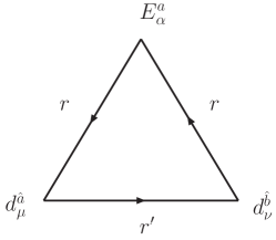
Figure 1: One-loop contribution to the Green function $\langle E^{a}_{\alpha}d^{\hat{a}}_{\mu}d^{\hat{b}}_{\nu}\rangle$ from composite fermions in the representations $r$ and $r^{\prime}$ of $SO(4)$.

For a given diagram with fermions in the representations $r$ and $r^{\prime}$ of $SO(4)$, the Feynman amplitude can be expressed as

$$M_{\alpha\mu\nu}^{a\hat{a}\hat{b}}=N_{\chi}\,\omega^{a\hat{a}\hat{b}}_{[r,r^{\prime}]}\,|\zeta_{[r,r^{\prime}]}|^{2}\,I_{\alpha\mu\nu}(p_{1},p_{2};m_{r},m_{r^{\prime}})\,,$$ (3.8)

where $p_{1}$ and $p_{2}$ are the momenta of $d_{\mu}^{\hat{a}}$ and $d_{\nu}^{\hat{b}}$ respectively (defined to be flowing into the corresponding vertices), the index $a$ runs over the adjoint of $SU(2)_{L}\times SU(2)_{R}$, and $N_{\chi}$ is the fermion multiplicity. For example, for three families of colored fermions (heavy quarks) one has $N_{\chi}=N_{c}N_{F}=9$ (with $N_{c}=3$, $N_{F}=3$), while $N_{\chi}=12$ if there are three additional families of colorless fermions (i.e. heavy leptons). Here $\zeta_{[r,r^{\prime}]}=\zeta_{[r^{\prime},r]}^{*}$ denotes the coupling strength of $d_{\mu}$ with fermions in the representations $r$ and $r^{\prime}$: $\zeta_{[(\mathbf{[},\mathbf{2})]{2},(\mathbf{[},\mathbf{1})]{1}]}=\zeta_{11}$, $\zeta_{[(\mathbf{[},\mathbf{2})]{2},(\mathbf{[},\mathbf{1})]{3}]}=\zeta_{13}$, and $\zeta_{[(\mathbf{[},\mathbf{2})]{2},(\mathbf{[},\mathbf{3})]{1}]}=\zeta_{31}$, as in Eq. (3.7). By $SO(4)$ covariance, the second factor of Eq. (3.8) is proportional to the $SO(4)$ generator $t^{a}_{\hat{a}\hat{b}}$,

$$\omega^{a_{L}\hat{a}\hat{b}}_{[r,r^{\prime}]}=l^{L}_{[r,r^{\prime}]}\,t^{a_{L}}_{\hat{a}\hat{b}}\,,\qquad\omega^{a_{R}\hat{a}\hat{b}}_{[r,r^{\prime}]}=l^{R}_{[r,r^{\prime}]}\,t^{a_{R}}_{\hat{a}\hat{b}}\,,$$ (3.9)

where the coefficients $l^{L,R}_{[r,r^{\prime}]}$ are reported in Table 1 for the fermion representations under study.

$[r,r^{\prime}]$	$[(\mathbf{[},\mathbf{2})]{2},(\mathbf{[},\mathbf{1})]{1}]$	$[(\mathbf{[},\mathbf{2})]{2},(\mathbf{[},\mathbf{1})]{3}]$	$[(\mathbf{[},\mathbf{1})]{3},(\mathbf{[},\mathbf{2})]{2}]$	$[(\mathbf{[},\mathbf{2})]{2},(\mathbf{[},\mathbf{3})]{1}]$	$[(\mathbf{[},\mathbf{3})]{1},(\mathbf{[},\mathbf{2})]{2}]$
$l^{L}_{[r,r^{\prime}]}$	$1$	$+3/4$	0	$-1/4$	$1$
$l^{R}_{[r,r^{\prime}]}$	$1$	$-1/4$	$1$	$+3/4$	0

Table 1: Value of the coefficients $l^{L,R}_{[r,r^{\prime}]}$ defined in Eq. (3.9) for diagrams with fermions in the $(\mathbf{[},\mathbf{1})]{1}$, $(\mathbf{[},\mathbf{2})]{2}$, $(\mathbf{[},\mathbf{1})]{3}$ and $(\mathbf{[},\mathbf{3})]{1}$ of $SO(4)\sim SU(2)_{L}\times SU(2)_{R}$. The coefficients not shown in the Table are vanishing.

The contribution to $c_{4}^{\pm}$ can be extracted by expanding the loop function $I_{\alpha\mu\nu}$ at first order in the external momenta. It is easy to show that $I_{\alpha\mu\nu}$ is antisymmetric under the exchange $\{\mu,p_{1}\}\leftrightarrow\{\nu,p_{2}\}$, so there are three possible Lorentz structures at linear order in the external momenta:

$$\begin{split}I_{\alpha\mu\nu}=\,&A(m_{r},m_{r^{\prime}})\,\eta_{\mu\nu}(p_{1}-p_{2})_{\alpha}+B(m_{r},m_{r^{\prime}})\left(p_{1\,\mu}\eta_{\nu\alpha}-p_{2\,\nu}\eta_{\mu\alpha}\right)\\[2.84544pt] &+C(m_{r},m_{r^{\prime}})\left[\eta_{\nu\alpha}(p_{1}+p_{2})_{\mu}-\eta_{\mu\alpha}(p_{1}+p_{2})_{\nu}\right]+O(p^{3})\,.\end{split}$$ (3.10)

The functions $A$, $B$, $C$ are logarithmically divergent and their expression is given in Appendix C. The terms proportional to $A$ and $B$ renormalize respectively the operators $O_{d1}=\text{Tr}[(\nabla_{\mu}d_{\nu})^{2}]$ and $O_{d2}=\text{Tr}[(\nabla_{\mu}d^{\mu})^{2}]$, which contain terms with zero, one and two $E_{\mu}$’s from the covariant derivative. In fact, the same function $I_{\alpha\mu\nu}$ accounts for the one-loop contribution to the three-point Green function $\langle J^{a}_{\alpha}d^{\hat{a}}_{\mu}d^{\hat{b}}_{\nu}\rangle$, where $J_{\mu}^{a}$ is the $SO(4)$ conserved current (see Eq. (D.3)). It is thus subject to the Ward identity

$$i(p_{1}+p_{2})^{\alpha}I_{\alpha\mu\nu}=G_{\mu\nu}(p_{1}^{2})-G_{\mu\nu}(p_{2}^{2})\,,$$ (3.11)

where $G_{\mu\nu}(p^{2})$ is the $d_{\mu}$ self-energy:

$$\langle d^{\hat{a}}_{\mu}d^{\hat{b}}_{\nu}\rangle|_{amp}\equiv\delta^{\hat{a}\hat{b}}G_{\mu\nu}(p^{2})=\delta^{\hat{a}\hat{b}}\eta_{\mu\nu}\,\Pi_{0}(p^{2})+\delta^{\hat{a}\hat{b}}p_{\mu}p_{\nu}\,\Pi_{1}(p^{2})\,.$$ (3.12)

From Eq. (3.11) it follows that

$$A(m_{r},m_{r^{\prime}})=\Pi_{0}^{\prime}(0)\,,\qquad B(m_{r},m_{r^{\prime}})=\Pi_{1}(0)\,.$$ (3.13)

We have checked these identities by explicitly computing the self-energy $G_{\mu\nu}$. The coefficients of the operators $O_{d1}$, $O_{d2}$ are given by

$$\begin{split}c_{d1}&=\frac{N_{\chi}}{4}\sum_{r,r^{\prime}}A(m_{r},m_{r^{\prime}})\left(l_{[r,r^{\prime}]}^{L}+l_{[r,r^{\prime}]}^{R}\right)\,|\zeta_{[r,r^{\prime}]}|^{2}\,,\\[4.26773pt] c_{d2}&=\frac{N_{\chi}}{4}\sum_{r,r^{\prime}}B(m_{r},m_{r^{\prime}})\left(l_{[r,r^{\prime}]}^{L}+l_{[r,r^{\prime}]}^{R}\right)\,|\zeta_{[r,r^{\prime}]}|^{2}\,,\end{split}$$ (3.14)

where the sums are over all possible fermion representations $r,r^{\prime}$ contributing to the 1-loop diagram of Fig. 1.  Neither of the operators $O_{d1}$, $O_{d2}$ contributes to $h\to Z\gamma$: $O_{d2}$ can be redefined away in terms of higher-derivative operators by using the equations of motion $\nabla_{\mu}d^{\mu}=0$, while $O_{d1}$ can be rewritten as

$$\text{Tr}[(\nabla_{\mu}d_{\nu})^{2}]\equiv O_{d1}=\frac{1}{2}\text{Tr}[F_{\mu\nu}^{2}]-\frac{1}{2}O_{3}^{+}+\frac{1}{4}\left(O_{2}-O_{1}\right)\,,$$ (3.15)

and thus contributes to the $S$ parameter. We will discuss this further in the next section, where we perform a detailed calculation of $S$.

Finally, the term proportional to $C$ in Eq. (3.10) renormalizes the operator $\text{Tr}[E_{\mu\nu}d^{\mu}d^{\nu}]$ and thus contributes to $c_{4}^{\pm}$. We find:

$$c_{4}^{\pm}=\frac{N_{\chi}}{4}\sum_{r,r^{\prime}}C(m_{r},m_{r^{\prime}})\left(l_{[r,r^{\prime}]}^{L}\pm l_{[r,r^{\prime}]}^{R}\right)\,|\zeta_{[r,r^{\prime}]}|^{2}\,.$$ (3.16)

Using the coefficients of Table 1 and Eqs. (C.3) and (2.6), one can derive the fermionic contribution to the $hZ\gamma$ vertex. In particular, in a theory with composite fermions only in the $(\mathbf{[},\mathbf{1})]{1}$ and $(\mathbf{[},\mathbf{2})]{2}$ representations, the contribution to $c_{4}^{-}$ (hence to $c_{Z\gamma}$) vanishes identically, since $l^{L}_{[(\mathbf{[},\mathbf{2})]{2},(\mathbf{[},\mathbf{1})]{1}]}=l^{R}_{[(\mathbf{[},\mathbf{2})]{2},(\mathbf{[},\mathbf{1})]{1}]}$ and $l^{L,R}_{[(\mathbf{[},\mathbf{1})]{1},(\mathbf{[},\mathbf{2})]{2}]}=0$. This is expected, since the fermionic sector in this case possesses an accidental $P_{LR}$ invariance. When fermions in the $(\mathbf{[},\mathbf{1})]{3}$ and $(\mathbf{[},\mathbf{3})]{1}$ are present, however, the contribution to $c_{4}^{-}$ is non-vanishing provided $P_{LR}$ is broken either by the couplings ($\zeta_{13}\not=\zeta_{31}$) or in the spectrum ($m_{(\mathbf{[},\mathbf{1})]{3}}\not=m_{(\mathbf{[},\mathbf{3})]{1}}$).

It is interesting to notice that although the function $C$ is logarithmically divergent, the contribution to $c_{4}^{-}$ from Eq. (3.16) is finite, since the coefficients $l_{[r,r^{\prime}]}^{L,R}$ satisfy the sum rule

$$\left(l_{[r,r^{\prime}]}^{L}-l_{[r,r^{\prime}]}^{R}\right)+\left(l_{[r^{\prime},r]}^{L}-l_{[r^{\prime},r]}^{R}\right)=0\hskip 28.45274pt\text{for any }r,r^{\prime}\,.$$ (3.17)

This identity can be directly checked on the coefficients of Table 1, and a simple argument shows that it holds in general for any pair $(r,r^{\prime})$. The proof goes as follows. When computing the 1-loop diagram of Fig. 1, it is useful to treat $E_{\mu}$ and $d_{\mu}$ as external backgrounds coupled to the fermions. Let us then turn on $E_{\mu}$ along the diagonal $U(1)_{L+R}$ subgroup of $SO(4)\sim SU(2)_{L}\times SU(2)_{R}$, under which $d_{\mu}^{1}\pm id_{\mu}^{2}$ has charge $\pm 1$ and $d_{\mu}^{3}$ and $d_{\mu}^{4}$ have charge $0$. By charge conservation there are only two possible diagrams (plus their crossings) as in Fig. 1: one with $d^{1}_{\mu}$ and $d^{2}_{\nu}$ at the two lower vertices, the other with $d^{3}_{\mu}$ and $d^{4}_{\nu}$. Since $d_{\mu}^{1,2,3}$ are odd while $d_{\mu}^{4}$ is even under $P_{LR}$, the second diagram contributes to $O_{4}^{-}$, while the first renormalizes $O_{4}^{+}$.  We thus concentrate on the diagram with $d^{3}_{\mu}d^{4}_{\nu}$ and notice that the fermions circulating in the loop must all have the same $U(1)_{L+R}$ charge. Let $\lambda_{ij}^{3}$ and $\lambda_{ij}^{4}$ be the coupling strengths of two same-charge fermions $i$ and $j$ respectively to $d_{\mu}^{3}$ and $d_{\mu}^{4}$ (in the fermions’ mass eigenbasis). For a given diagram with fermions $i$ and $j$ in the loop, the log-divergent part is thus proportional to $(\lambda^{3}_{ij}\lambda^{4}_{ji})$. Due to the antisymmetry of the loop function, $I_{\alpha\mu\nu}(p_{1},p_{2},m_{i},m_{j})=-I_{\alpha\nu\mu}(p_{2},p_{1},m_{i},m_{j})$, the log-divergent part of the crossed diagram is instead proportional to $-(\lambda^{4}_{ij}\lambda^{3}_{ji})$. The sum then vanishes after summing over all fermions $i$, $j$ with the same charge. This proves that there is no log-divergent contribution to $c_{4}^{-}$ from 1-loop fermion diagrams, hence the sum rule (3.17) must hold for any pair of $SO(4)$ representations $(r,r^{\prime})$. In general, a logarithmic divergence $\log(\Lambda/m)$ is associated with the running of a Wilson coefficient from the cutoff scale $\Lambda$ down to the fermion mass scale $m$. The above argument thus shows that there is no RG running of $c_{4}^{-}$ induced by 1-loop diagrams of fermions above their mass scale, while such running is present in general for $c_{4}^{+}$.

So far we have considered 1-loop diagrams with only composite fermions. There are also diagrams where both fermions and spin-1 resonances can circulate. At the 1-loop level, however, $\rho^{L,R}$ can only appear external to the loop due to the mixing with $E_{\mu}$ from its mass term and a coupling to the fermions of the form

$$\bar{\chi}_{r}\left(\rho_{\mu}-E_{\mu}\right)\gamma^{\mu}\chi_{r}\,.$$ (3.18)

The corresponding diagram is shown in Fig. 2.

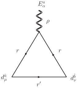
Figure 2: Mixed rho-fermion contribution to the Green function $\langle E^{a}_{\alpha}d^{\hat{a}}_{\mu}d^{\hat{b}}_{\nu}\rangle$ which arises at the one-loop level.

It is easy to see that its contribution to $c_{4}^{-}$ vanishes at leading order: integrating out the $\rho$ through the equations of motion generates only four-fermion operators, which in turn do not contribute at the 1-loop level. In general, the tree-level exchange of the $\rho$ in the diagram of Fig. 2 leads to a form-factor correction to the vertex of $E_{\mu}$ with the fermionic current. For $q^{2}=(p_{1}+p_{2})^{2}\ll m_{\rho}^{2}$ such a form factor correction is of order $q^{2}/m_{\rho}^{2}$ and is thus suppressed compared to the direct interaction from the fermions’ kinetic terms.

3.3 Two models

We have already alluded to the fact that a generic $P_{LR}$-violating strong dynamics can lead to unacceptably large corrections to the $Z\bar{b}b$ vertex [14]. Here we sketch two simple models where the breaking of $P_{LR}$ is communicated to the $Z\bar{b}b$ vertex in a suppressed way, such that a sizable correction to $h\to Z\gamma$ is phenomenologically allowed.

Model 1

In the first model, which is a low-energy simplified version of the MCHM5 [16], the composite fermions fill two fundamental representations of $SO(5)$, with $U(1)_{X}$ charge $+2/3$ and $-1/3$ respectively:

$$\begin{split}\chi_{5}&=(\mathbf{[},\mathbf{1})]{1}_{2/3}+(\mathbf{[},\mathbf{2})]{2}_{2/3}\\[2.84544pt] \chi^{\prime}_{5}&=(\mathbf{[},\mathbf{1})]{1}_{-1/3}+(\mathbf{[},\mathbf{2})]{2}_{-1/3}\,.\end{split}$$ (3.19)

The spectrum of composite states also includes a $\rho^{L}$ and $\rho^{R}$, while we omit for simplicity spin-1 states transforming as bifundamentals of $SU(2)_{L}\times SU(2)_{R}$. The Lagrangian can be written as ${\cal L}={\cal L}_{elem}+{\cal L}_{comp}+{\cal L}_{mix}$, where ${\cal L}_{elem}$ describes the elementary fields in isolation and the expression of the composite Lagrangian ${\cal L}_{comp}$ is as in Eqs. (3.2) and (3.7). The term ${\cal L}_{mix}$ accounts for the mixing of the elementary to composite fermions:

$${\cal L}_{mix}=\lambda_{q}\,\bar{q}_{L}P_{q}U(\pi)\chi_{5}+\lambda^{\prime}_{q}\,\bar{q}_{L}P_{q}U(\pi)\chi_{5}^{\prime}+\lambda_{t}\,\bar{t}_{R}P_{t}U(\pi)\chi_{5}+\lambda_{b}\,\bar{b}_{R}P_{b}U(\pi)\chi_{5}^{\prime}+h.c.\,,$$ (3.20)

where $P_{q,t,b}$ project out the components of the composite fields with the electroweak quantum numbers of the corresponding elementary fields. The $P_{LR}$ invariance is taken to be maximally violated in the spin-1 sector, but is accidentally preserved in the fermion sector. If $\lambda_{q}^{\prime}\ll\lambda_{q}$, then the $Z\bar{b}b$ coupling is protected from large corrections since for $\lambda_{q}^{\prime}=0$ there is no operator at leading order in the derivative expansion which can modify it [15]. A small $\lambda_{q}^{\prime}/\lambda_{q}$ can in fact naturally arise from the RG running of the full theory and explain the hierarchy between the top and bottom masses if $\lambda_{t}\simeq\lambda_{b}$ [16]. We note in passing that at tree level the correction to $Z\bar{b}b$ from a $\rho^{L,R}$ is always vanishing at leading order in the derivative expansion, as can be easily checked by using the equations of motion $\rho_{\mu}=E_{\mu}+O(p^{3})$ in Eq. (3.18). This is because the shift induced by the exchange of the $\rho$ is exactly compensated by the additional interaction $\bar{\chi}\gamma^{\mu}E_{\mu}\chi=\bar{\chi}\gamma^{\mu}(H^{\dagger}i{\overleftrightarrow{D_{\mu}}}H+\dots)\chi$ required by $SO(5)$ invariance and included in the term of Eq. (3.18). A non-vanishing $Z\bar{b}b$ will however arise in general at the 1-loop level in absence of a symmetry protection. In the model under consideration such a protection comes from the accidental $P_{LR}$-symmetry of the fermionic sector, which also implies that the vertex $hZ\gamma$ in this case is generated only by the $\rho$ exchange; the value of $c_{Z\gamma}$ is thus given by Eq. (3.6).

Model 2

In the second model the composite fermions fill one fundamental plus one antisymmetric representation of $SO(5)$, with $U(1)_{X}$ charge $+2/3$ and $-1/3$ respectively:

$$\begin{split}\chi_{5}&=(\mathbf{[},\mathbf{1})]{1}_{2/3}+(\mathbf{[},\mathbf{2})]{2}_{2/3}\\[2.84544pt] \chi_{10}&=(\mathbf{[},\mathbf{2})]{2}_{-1/3}+(\mathbf{[},\mathbf{1})]{3}_{-1/3}+(\mathbf{[},\mathbf{3})]{1}_{-1/3}\,.\end{split}$$ (3.21)

As before, the Lagrangian can be divided into an elementary and a composite part plus a mixing term

$$\begin{split}{\cal L}_{mix}=&\,\lambda^{10}_{q}\,\bar{q}_{L}P_{q}U(\pi)\chi_{10}+\lambda^{5}_{q}\,\bar{q}_{L}P_{q}U(\pi)\chi_{5}+\lambda^{10}_{t}\,\bar{t}_{R}P_{t}U(\pi)\chi_{10}\\ &+\lambda^{5}_{t}\,\bar{t}_{R}P_{t}U(\pi)\chi_{5}+\lambda_{b}\,\bar{b}_{R}P_{b}U(\pi)\chi_{10}+h.c.\,.\end{split}$$ (3.22)

In this case the fermionic sector is not in general $P_{LR}$ invariant, so both loops of composite fermions and the tree-level exchange of the $\rho$ can contribute to generate the $hZ\gamma$ vertex. Using Eqs. (3.6), (3.16) and (2.6) we find

$$\begin{split}c_{Z\gamma}=&\,\frac{g^{2}}{2}\sin^{2}\!\theta\,(\alpha_{1L}-\alpha_{1R})\\ &+\frac{g^{2}}{4}N_{\chi}\sin^{2}\!\theta\,\Big{[}|\zeta_{13}|^{2}\left(C(m_{(\mathbf{[},\mathbf{2})]{2}},m_{(\mathbf{[},\mathbf{1})]{3}})-C(m_{(\mathbf{[},\mathbf{1})]{3}},m_{(\mathbf{[},\mathbf{2})]{2}})\right)\\ &\hskip 76.82234pt-|\zeta_{31}|^{2}\left(C(m_{(\mathbf{[},\mathbf{2})]{2}},m_{(\mathbf{[},\mathbf{3})]{1}})-C(m_{(\mathbf{[},\mathbf{3})]{1}},m_{(\mathbf{[},\mathbf{2})]{2}})\right)\Big{]}\,.\end{split}$$ (3.23)

The shift to $Z\bar{b}b$ is suppressed for $\lambda_{q}^{10}$ small, since no effect can arise from the $P_{LR}$-preserving coupling $\lambda_{q}^{5}$ [14]. As before, a small $\lambda_{q}^{10}/\lambda_{q}^{5}$ can arise naturally from the RG flow of the full theory, and can explain the hierarchy between the top and bottom masses if $\lambda_{t}^{10}\ll\lambda_{t}^{5}\simeq\lambda_{b}$.

4 $S$ parameter from loops of fermionic resonances

In the previous Section we have seen that loops of composite fermions generate the operator $O_{d1}$ through the triangle diagram of Fig. 1; the value of the corresponding coefficient $c_{d1}$ is given by Eq. (3.14). Since $O_{d1}$ can be rewritten in terms of $O_{3}^{+}$ as in Eq. (3.15), it contributes to the $S$ parameter. As implied by the Ward identity (3.11), the same contribution to $c_{d1}$, hence to $S$, can be derived by considering the $\langle d_{\mu}d_{\nu}\rangle$ self-energy diagram shown on the left of Fig. 3, where two different $SO(4)$ representations of fermions circulate in the loop.

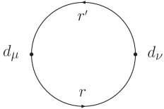
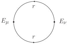
Figure 3: One loop diagrams contributing to the $\langle d_{\mu}d_{\nu}\rangle$ (left) and $\langle E_{\mu}E_{\nu}\rangle$ (right) self-energies.

There is however an additional direct contribution to $O_{3}^{\pm}$ which comes from the $\langle E_{\mu}E_{\nu}\rangle$ self-energy diagram shown on the right of Fig. 3, where a single fermion representation $r$ appears in the loop. Summing over $r$, we find

$$c_{3}^{\pm}=\frac{N_{\chi}}{8}\sum_{r}(C_{L}[r]\pm C_{R}[r])A(m_{r},m_{r})\,,$$ (4.1)

where for the fundamental representation $C_{L}[(\mathbf{[},\mathbf{2})]{2}]=C_{R}[(\mathbf{[},\mathbf{2})]{2}]=1$, for the adjoint $C_{R}[(\mathbf{[},\mathbf{1})]{3}]=C_{L}[(\mathbf{[},\mathbf{3})]{1}]=2$ and $C_{L}[(\mathbf{[},\mathbf{1})]{3}]=C_{R}[(\mathbf{[},\mathbf{3})]{1}]=0$, while $C_{L,R}[(\mathbf{[},\mathbf{1})]{1}]=0$. The total contribution to the $S$ parameter from loops of composite fermions is thus

$$\Delta S=-4\pi N_{\chi}\sin^{2}\!\theta\left[\sum_{r}(C_{L}[r]+C_{R}[r])A(m_{r},m_{r})-\sum_{r,r^{\prime}}|\zeta_{[r,r^{\prime}]}|^{2}C[r,r^{\prime}]A(m_{r},m_{r^{\prime}})\right]\,,$$ (4.2)

where we have conveniently defined $C[r,r^{\prime}]=(1/2)(l_{[r,r^{\prime}]}^{L}+l_{[r,r^{\prime}]}^{R}+l_{[r^{\prime},r]}^{L}+l_{[r^{\prime},r]}^{R})$ and used the fact that the function $A(m_{r},m_{r^{\prime}})$ is symmetric in its arguments. For example, in the first model discussed in Section 3.3 with fermions in the $(\mathbf{[},\mathbf{1})]{1}$ and $(\mathbf{[},\mathbf{2})]{2}$ of $SO(4)$ one has

$$\begin{split}\Delta S&=-8\pi N_{\chi}\sin^{2}\!\theta\left(A(m_{(\mathbf{[},\mathbf{2})]{2}},m_{(\mathbf{[},\mathbf{2})]{2}})-|\zeta_{11}|^{2}A(m_{(\mathbf{[},\mathbf{2})]{2}},m_{(\mathbf{[},\mathbf{1})]{1}})\right)\\[5.69046pt] &=\frac{2}{3}\,\frac{N_{\chi}}{\pi}\,\frac{v^{2}}{f^{2}}\left(1-|\zeta_{11}|^{2}\right)\log\!\bigg{(}\frac{\Lambda^{2}}{\bar{m}^{2}}\bigg{)}+\text{finite terms}\,,\end{split}$$ (4.3)

where in the second expression $\bar{m}$ denotes an average mass and the finite terms include the proper ratios of fermion masses. In the second model with fermions in the $(\mathbf{[},\mathbf{2})]{2}$, $(\mathbf{[},\mathbf{1})]{3}$ and $(\mathbf{[},\mathbf{3})]{1}$ we find

$$\begin{split}\Delta S&=-8\pi N_{\chi}\sin^{2}\!\theta\,\bigg{[}A(m_{(\mathbf{[},\mathbf{2})]{2}},m_{(\mathbf{[},\mathbf{2})]{2}})+A(m_{(\mathbf{[},\mathbf{3})]{1}},m_{(\mathbf{[},\mathbf{3})]{1}})+A(m_{(\mathbf{[},\mathbf{1})]{3}},m_{(\mathbf{[},\mathbf{1})]{3}})\\ &\phantom{=-8\pi N_{\chi}\sin^{2}\!\theta\,\bigg{[}\,}-\frac{3}{2}|\zeta_{13}|^{2}A(m_{(\mathbf{[},\mathbf{2})]{2}},m_{(\mathbf{[},\mathbf{1})]{3}})-\frac{3}{2}|\zeta_{31}|^{2}A(m_{(\mathbf{[},\mathbf{2})]{2}},m_{(\mathbf{[},\mathbf{3})]{1}})\bigg{]}\\[5.69046pt] &=\frac{1}{2}\,\frac{N_{\chi}}{\pi}\,\frac{v^{2}}{f^{2}}\left(2-|\zeta_{13}|^{2}-|\zeta_{31}|^{2}\right)\log\!\bigg{(}\frac{\Lambda^{2}}{\bar{m}^{2}}\bigg{)}+\text{finite terms}\,.\end{split}$$ (4.4)

From Eqs.(4.2)-(4.4) one can see that the $S$ parameter is in general logarithmically divergent, as expected on dimensional grounds. The coefficient of the log can be either positive or negative depending on the value of the parameters $\zeta$. Analogous results were first obtained in the context of Technicolor theories in Ref. [22] and later re-derived for $SO(4)/SO(3)$ Higgsless models by Ref. [23]. More recently, the case of $SO(5)/SO(4)$ composite Higgs theories has been discussed in Ref. [24].  A simple way to understand why the log divergence vanishes if the parameters $\zeta$ are equal to 1 is by noticing that in this limit the Lagrangian (3.7) can be rewritten, through a field redefinition, as the Lagrangian of a two-site model where the Higgs couplings to the composite fermions are non-derivative.  This implies, by simple inspection of the relevant one-loop diagrams, that the $S$ parameter is finite in this case. For completeness we report in Appendix E a short discussion on the connection between the CCWZ Lagrangian (3.7) and that of the two-site model.

The fact that the overall sign of $S$ is controlled by the coefficients $\zeta$ and can be negative is more clearly understood by considering the dispersion relation obeyed by $S$ [20]:

$$S=4\pi\sin^{2}\!\theta\int\!\frac{ds}{s}\left[\rho_{LL}(s)+\rho_{RR}(s)-2\rho_{BB}(s)\right]\,,$$ (4.5)

where $\rho_{LL}$, $\rho_{RR}$ and $\rho_{BB}$ are the spectral functions respectively of two unbroken ($SU(2)_{L}$ and $SU(2)_{R}$) and broken ($SO(5)/SO(4)$) conserved currents of the strong sector. The definition of the spectral function $\rho(s)$ and the expression of the currents is reported in Appendix D for completeness. From Eq. (4.5) and from the positivity of each individual spectral function, it is clear that a negative $S$ can occur if $\rho_{BB}$ is sufficiently large. The leading contribution of the fermions to the spectral functions can be easily computed from the diagrams shown in Fig. 4. We find:

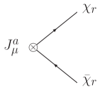
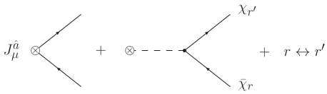
Figure 4: Two-particle contribution to the spectral function of unbroken (upper row) and broken (lower row) currents from the composite fermions. The dashed line denotes the propagator of a NG boson.

$$\begin{split}\rho_{LL,RR}(q^{2})&=\frac{1}{12\pi^{2}}\sum_{r}C_{L,R}[r]\,\lambda(q^{2},m_{r},m_{r})\\[5.69046pt] \rho_{BB}(q^{2})&=\frac{1}{24\pi^{2}}\sum_{r,r^{\prime}}|\zeta_{[r,r^{\prime}]}|^{2}C[r,r^{\prime}]\,\lambda(q^{2},m_{r},m_{r^{\prime}})\,,\end{split}$$ (4.6)

where we have defined

$$\begin{split}\lambda(q^{2},m_{r},m_{r^{\prime}})=&\,\left(1-\frac{(m_{r}-m_{r^{\prime}})^{2}}{q^{2}}\right)\left(1+\frac{(m_{r}+m_{r^{\prime}})^{2}}{2q^{2}}\right)\\[2.84544pt] &\times\sqrt{\left(1+\frac{m_{r}^{2}-m_{r^{\prime}}^{2}}{q^{2}}\right)^{2}-4\,\frac{m_{r}^{2}}{q^{2}}}\,.\end{split}$$ (4.7)

By inserting these expressions into the dispersion relation (4.5), one re-obtains the result of Eq. (4.2). Since $\rho_{BB}$ is proportional to $|\zeta_{[r,r^{\prime}]}|^{2}$, it is clear that for sufficiently large $|\zeta_{[r,r^{\prime}]}|$ the $S$ parameter will become negative.

5 Numerical Results and Discussion

In this paper we have focused on the virtual effects due to purely composite states. The Higgs decay rate to $Z\gamma$ and the $S$ parameter are two low-energy observables extremely sensitive to such effects.  It is well know that the tree-level contribution to $S$ from spin-1 resonances is large and poses tight constraints on the scale of compositeness. We have seen that the exchange of $\rho^{L}$ and $\rho^{R}$ generates the effective interaction $hZ\gamma$ also at tree level, provided their masses and couplings are not $P_{LR}$ symmetric. This leads to a correction to the $h\to Z\gamma$ decay rate that is potentially larger than that due to the $O(v^{2}/f^{2})$ shifts in the tree-level Higgs couplings from the non-linear $\sigma$-model Lagrangian. This is the case unless the coefficients of the operators $Q_{1L}$ and $Q_{1R}$ are loop suppressed, as happens for example in Holographic Higgs theories. The contribution from fermionic resonances arises at the 1-loop level, and can be numerically large. The main reason for this is that loops of pure composites are sensitive to the multiplicity of states arising from the strong dynamics. In particular all the composite fermion species, including the partners of SM light quarks and leptons, will circulate in the loop regardless of how strongly mixed with the elementary fermions they are. The multiplicity factor $N_{\chi}$ can then partly compensate for the one-loop suppression, giving large shifts to both the $S$ parameter and the $h\to Z\gamma$ rate. 

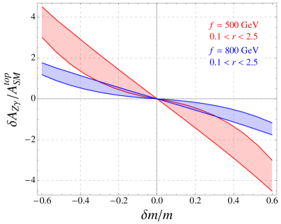
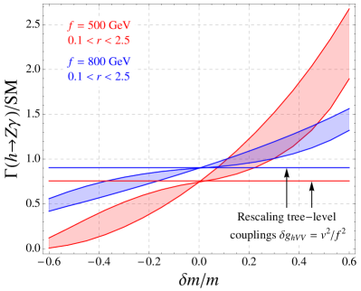
Figure 5: Left plot: shift of the $h\to Z\gamma$ decay amplitude in units of the SM top contribution, $\delta A/A^{top}_{SM}$, in the second model of Section 3.3 as a function of the $LR$ mass splitting. Right plot: total decay rate of $h\to Z\gamma$ normalized to its SM value, $\Gamma/\Gamma_{SM}$, in the same model. The left plot assumes one family of colored fermions ($N_{\chi}=3$), while the right plot assumes three degenerate families of composites ($N_{\chi}=9$). The horizontal lines indicate the value obtained by including only the effect of the modified tree-level Higgs couplings.

To illustrate the size of the effects we have been discussing, the left plot of Fig. 5 shows the shift to the $h\to Z\gamma$ decay amplitude in units of the SM top contribution, $\delta A/A^{top}_{SM}$, due to one family of colored fermions (composite quarks) transforming as a $\mathbf{10}+\mathbf{5}$ of $SO(5)$ (second model of Section 3.3 with $N_{\chi}=3$). As discussed in Section 3.2, the correction comes entirely from the $\mathbf{10}$, hence the relevant parameters are the following: the scale of compositeness $f$, the coefficients $\zeta_{13}$, $\zeta_{31}$, and two ratios of masses which we conveniently define to be $\delta m/m\equiv(m_{(\mathbf{[},\mathbf{3})]{1}}-m_{(\mathbf{[},\mathbf{1})]{3}})/(m_{(\mathbf{[},\mathbf{3})]{1}}+m_{(\mathbf{[},\mathbf{1})]{3}})$ and $r\equiv m_{(\mathbf{[},\mathbf{2})]{2}}/(m_{(\mathbf{[},\mathbf{3})]{1}}+m_{(\mathbf{[},\mathbf{1})]{3}})$. For simplicity we fix $\zeta_{13}=\zeta_{31}=1$, so that the amount of $P_{LR}$ breaking is fully controlled by $\delta m/m$. The plot shows the relative shift $\delta A/A^{top}_{SM}$ as a function of $\delta m/m$ for two representative values $f=500\,$GeV and $f=800\,$GeV. The red and blue bands are obtained by varying $r$ in the interval $0.1<r<2.5$. By rescaling $\zeta_{13}$ and $\zeta_{31}$ by a common factor $\zeta$, $\delta A$ goes like $\zeta^{2}$, though even without such an enhancement we see that shifts of several times the SM top amplitude are possible for large mass splittings. The right plot of Fig. 5 shows the total decay rate normalized to its SM value, this time for three degenerate families of colored fermions (second model of Section 3.3 with $N_{\chi}=9$). The horizontal lines indicate the value obtained by including only the effect of the modified tree-level Higgs couplings discussed above. Since in the SM the $W$ loop contribution largely dominates that of the top quark, the effect from the modified tree-level couplings is a suppression of the decay rate by a factor $(g_{WWh}/g_{WWh}^{SM})^{2}=(1-v^{2}/f^{2})$. The correction from the 1-loop exchange of composite fermions is included in addition to this effect, and can further suppress or enhance the decay rate depending on the sign of the mass splitting $\delta m/m$.

It is interesting to derive the contribution to the $S$ parameter in this model and analyze the impact of a sizable correction to the $h\to Z\gamma$ decay rate on the EWPT. This is illustrated by Fig. 6 in the $(S,T)$ plane.  The plot shows the region spanned by varying $f$ and $\zeta\equiv\zeta_{13}=\zeta_{31}=\zeta_{11}$ due to the IR correction to $S$ and $T$ from modified Higgs couplings and to the 1-loop correction to $S$ from three degenerate families of composite fermions (Eqs. (4.3) and (4.4) with $N_{\chi}=9$).

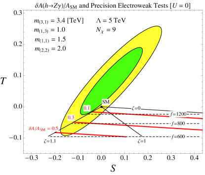
Figure 6: Region spanned in the plane $(S,T)$ when varying $f$ and $\zeta=\zeta_{13}=\zeta_{31}=\zeta_{11}$ in the second model of Section 3.3, as due to $\Delta S$ from loops of composite fermions and to the IR correction to $S$ and $T$ from modified Higgs couplings. The green and yellow areas indicate the regions with 68% and 95% probability [29]. Dashed (solid black) lines indicate the trajectories of fixed $f$ ($\zeta$). The thicker solid red lines indicate the isocurves of constant $h\to Z\gamma$ decay amplitude.

We have fixed the cutoff scale to $\Lambda=5\,$TeV, and have chosen the following spectrum of composite masses: $m_{(\mathbf{[},\mathbf{1})]{1}}=1.5\,$TeV, $m_{(\mathbf{[},\mathbf{2})]{2}}=2.0\,$TeV, $m_{(\mathbf{[},\mathbf{3})]{1}}=3.4\,$TeV, $m_{(\mathbf{[},\mathbf{1})]{3}}=1.0\,$TeV, so that $r=0.45$ and $\delta m/m=0.55$. Even in the absence of additional contributions to $T$, the correction to $S$ from loops of composite fermions can compensate the shift due to the modified couplings of the Higgs to the SM vector bosons and bring the theory point back into the $95\%$ probability contour. For example, for $f=800\,$GeV (i.e. $(v/f)^{2}\simeq 0.09$) one has $\Delta S\simeq 0.83\,(1-\zeta^{2})$ from composite fermions, so that $\zeta\sim 1.1$ gives $\Delta S\sim-0.2$ as required to offset the IR shift. Correspondingly, the correction to the $h\to Z\gamma$ rate is sizable and of order $70\%$ of the SM value. In general, the 1-loop contribution to $S$ is large and only values $\zeta\simeq 1$ are viable. The fact that EWPT select a narrow range of $\zeta$ is directly relevant for the experimental searches of the fermionic resonances, since $\zeta$ controls their single production [28].  The exact allowed range depends however on possible additional contributions to $S$ and $T$. For example, for $g_{\rho_{L}}=3$ and $f=800\,$GeV the contribution to $S$ from a $\rho^{L}$ is $\Delta S\simeq 0.13$ (see Eq. (3.5)), which increases the preferred value of $\zeta$ by only a $5-10\%$, which in turn corresponds to an increase of the $h\to Z\gamma$ rate by $10-20\%$.

The tuning required to comply with the EW precision tests can be alleviated if an additional positive contribution to $T$ is present. This can arise from loops of fermionic resonances, as recently discussed by Ref. [24]; see also Refs. [31]. Unlike the $S$ parameter, however, $T$ is generated only if the custodial invariance of the strong dynamics is broken, and therefore no correction can come from purely composite states. In theories with partial compositeness and flavor anarchy of the strong sector, the leading contribution arises from loops of elementary top quarks. For example, if $t_{R}$ mixes with a composite singlet of $SU(2)_{L}\times SU(2)_{R}$, as in model 1 of Section 3.3, the only breaking of custodial symmetry in the fermionic sector comes from $\lambda_{q}$. As a spurion analysis shows [7], one needs four powers of $\lambda_{q}$ to generate $T$, which implies a finite result (i.e. independent of the cutoff scale $\Lambda$). A subleading contribution comes from loops of spin-1 resonances and elementary hypercharge vector bosons. In this case the breaking of custodial symmetry comes from the hypercharge coupling, and two powers of $g^{\prime}$ are sufficient to generate $T$. Table 2 summarizes the naive estimates of the corrections to $\hat{S}\equiv(\alpha_{em}/4\sin^{2}\!\theta_{W})S$ and $\hat{T}\equiv\alpha_{em}T$.

		$\Delta\hat{S}$	$\Delta\hat{T}$
UV	$\chi$	$\displaystyle N_{\chi}\frac{g^{2}}{16\pi^{2}}\left(\frac{v^{2}}{f^{2}}\right)\log\!\left(\frac{\Lambda}{M}\right)$	$\displaystyle N_{c}\frac{\lambda_{q}^{2}}{16\pi^{2}}\left(\frac{v^{2}}{f^{2}}\right)\frac{\lambda_{q}^{2}}{g_{*}^{2}}$
	$\rho$	$\displaystyle\left(\frac{v^{2}}{f^{2}}\right)\left(\frac{g^{2}}{g_{*}^{2}}\right)$	$\displaystyle\frac{g^{\prime 2}}{16\pi^{2}}\left(\frac{v^{2}}{f^{2}}\right)\log\!\left(\frac{\Lambda}{M}\right)$
IR	NGB	$\displaystyle\frac{g^{2}}{16\pi^{2}}\left(\frac{v^{2}}{f^{2}}\right)\log\!\left(\frac{M}{\mu}\right)$	$\displaystyle\frac{g^{\prime 2}}{16\pi^{2}}\left(\frac{v^{2}}{f^{2}}\right)\log\!\left(\frac{M}{\mu}\right)$
	top	$\displaystyle N_{c}\frac{g^{2}}{16\pi^{2}}\left(\frac{v^{2}}{f^{2}}\right)\frac{\lambda_{q}^{2}}{g_{*}^{2}}\log\!\left(\frac{M}{\mu}\right)$	$\displaystyle N_{c}\frac{y_{t}^{2}}{16\pi^{2}}\left(\frac{v^{2}}{f^{2}}\right)\frac{\lambda_{q}^{2}}{g_{*}^{2}}\log\!\left(\frac{M}{\mu}\right)$

Table 2: Naive estimates of the UV corrections (from composite fermions $\chi$ and spin-1 resonances $\rho$) and IR corrections (from NG bosons and the top quark) to $\hat{S}\equiv(\alpha_{em}/4\sin^{2}\!\theta_{W})S$ and $\hat{T}\equiv\alpha_{em}T$.

As before, $g_{*}\sim M/f\sim g_{\rho}$ denotes the coupling strength of the composite states and $M$ their mass scale. The first two lines show the corrections discussed above that arise from the exchange of composite fermions and spin-1 resonances. These are short-distance effects at the scale $M$, which in the language of the Higgs effective Lagrangian correspond to threshold corrections to the Wilson coefficients $\bar{c}_{W}+\bar{c}_{B}$ and $\bar{c}_{T}$; see Ref. [6]. There are however additional contributions which are generated by the exchange of light SM fields below $M$ and are thus associated to the RG evolution of the Wilson coefficients down to IR scales $\mu\approx m_{Z}$. The largest corrections arise from loops of NG bosons (i.e. longitudinally polarized $W$ and $Z$ and the Higgs boson) and of top quarks, and correspond to the RG evolution of $\bar{c}_{W}+\bar{c}_{B}$ and $\bar{c}_{T}$ due to $\bar{c}_{H}$ and $\bar{c}_{H\psi}$, respectively [6]. Their naive estimates are reported in the last two lines of Table 2. Loops of transverse gauge bosons also lead to IR corrections which are subleading. For example, as recently pointed out by the authors of Ref. [32], 1-loop diagrams featuring one insertion of the effective $hZ\gamma$ vertex (induced by the operator $O_{HW}-O_{HB}$) give a correction to the $\hat{S}$ parameter of order

$$\Delta\hat{S}\sim\left(\frac{g^{2}}{16\pi^{2}}\right)^{2}\left(\frac{v^{2}}{f^{2}}\right)\log\!\left(\frac{M}{\mu}\right)^{2}\,.$$ (5.1)

Although directly linked to $h\to Z\gamma$, this is a two-loop EW effect which is parametrically subleading compared to other IR effects and numerically smaller than the UV corrections from pure composite fermions (see Table 2).

We briefly summarize our findings with the following conclusions:

• The decay mode $h\to Z\gamma$, unlike other loop-mediated processes of a Nambu-Goldstone composite Higgs, is subject to NP corrections that are not suppressed by the Goldstone symmetry itself. While new contributions to the $hgg$ and $h\gamma\gamma$ contact interactions of the effective Lagrangian are typically (and observably) small, a highly nonstandard $hZ\gamma$ interaction is possible and consistent with the symmetry that is assumed to be responsible for stabilizing the weak scale.

• Generating a large $hZ\gamma$ interaction in the absence of significant breaking of the Goldstone symmetry relies on the intervention of states arising from a strong sector that breaks a left-right symmetry, $P_{LR}$. Provided this breaking is mediated in a suppressed way to the $Zb\bar{b}$ coupling, as in the case of the models presented above, enhancements of $h\to Z\gamma$ remain phenomenologically viable.

• There are two operators contributing to the $S$ parameter that are closely related to those governing $h\to Z\gamma$, and a naive prediction would be for a tight correlation between these two observables. However, the composite Higgs can couple to fermions through interactions that contribute only to the two-point function of two broken currents, allowing an offsetting (negative) contribution to $S$ such that again the viability of large corrections in $h\to Z\gamma$ is retained.

In this paper we have highlighted the anatomy of the $h\to Z\gamma$ channel, one in which a composite Higgs might naturally interact in a novel way that could help shed light on its origins in the absence of other, more obvious, clues. As such, this channel deserves our full attention in the continuation of Higgs study at the LHC.

Appendix A Formulas for the $h\to Z\gamma$ decay rate

We collect here the formulas useful for the calculation of the decay rate $h\to Z\gamma$. The partial width is given by

$$\Gamma(h\to Z\gamma)=\frac{1}{32\pi}\frac{m_{h}^{3}}{v^{2}}\left(1-\frac{m_{Z}^{2}}{m_{h}^{2}}\right)^{3}\left|A\right|^{2}\,,$$ (A.1)

where $A$ is the total decay amplitude. The SM contribution arises from loops of $W$ vector bosons and fermions:

$$\begin{split}A_{SM}=&A_{F}+A_{W}\\[14.22636pt] A_{F}=&-\frac{\alpha_{em}}{\pi}\sum_{f}N_{cf}Q_{f}\frac{\left(T_{f}^{3L}-2Q_{f}\sin^{2}\theta_{W}\right)}{\sin\theta_{W}\cos\theta_{W}}\left[I_{1}(\tau_{f},\lambda_{f})-I_{2}(\tau_{f},\lambda_{f})\right]\\[7.11317pt] A_{W}=&-\frac{\alpha_{em}}{2\pi}\cot\theta_{W}\,\bigg{\{}4(3-\tan^{2}\theta_{W})I_{2}(\tau_{W},\lambda_{W})\\ &\hskip 79.6678pt+\left[\left(1+\frac{2}{\tau_{W}}\right)\tan^{2}\!\theta_{W}-\left(5+\frac{2}{\tau_{W}}\right)\right]I_{1}(\tau_{W},\lambda_{W})\bigg{\}}\,,\end{split}$$ (A.2)

where $N_{cf}$ and $Q_{f}$ are respectively the number of color and the electromagnetic charge of the fermion $f$, and we have defined

$$\tau_{f}\equiv\frac{4m_{f}^{2}}{m_{h}^{2}}\,,\qquad\lambda_{f}=\frac{4m_{f}^{2}}{m_{Z}^{2}}\,,\qquad\tau_{W}=\frac{4m_{W}^{2}}{m_{h}^{2}}\,,\qquad\lambda_{W}=\frac{4m_{W}^{2}}{m_{Z}^{2}}\,.$$ (A.3)

The loop functions are equal to

$$\begin{split}I_{1}(a,b)&=\frac{ab}{2(a-b)}+\frac{a^{2}b^{2}}{2(a-b)^{2}}\,(f(a)-f(b))+\frac{a^{2}b}{(a-b)^{2}}\,(g(a)-g(b))\\[4.26773pt] I_{2}(a,b)&=-\frac{ab}{2(a-b)}\left(f(a)-f(b)\right)\\[11.38092pt] g(\tau)&=\begin{cases}\sqrt{\tau-1}\,\arcsin(1/\sqrt{\tau}),&\tau\geq 1\\[2.84544pt] \frac{1}{2}\sqrt{1-\tau}\left[\log(\eta_{+}/\eta_{-})-i\pi\right],&\tau<1\end{cases}\\[11.38092pt] f(\tau)&=\begin{cases}\left[\arcsin(1/\sqrt{\tau})\right]^{2},&\tau\geq 1\\[2.84544pt] -{\displaystyle\frac{1}{4}}\left[\log(\eta_{+}/\eta_{-})-i\pi\right]^{2},&\tau<1\,,\end{cases}\end{split}$$ (A.4)

where $\eta_{\pm}\equiv(1\pm\sqrt{1-\tau})$. In the limit in which the New Physics effect can be parametrized by the effective Lagrangian of Eq. (1.3), the contribution to the decay amplitude is given by

$$A_{NP}=-2c_{Z\gamma}\,.$$ (A.5)

Numerically evaluating the SM contribution one finally obtains [6]:

$$\frac{\Gamma(h\rightarrow Z\gamma)}{\Gamma(h\rightarrow Z\gamma)_{SM}}\simeq\left|1+0.01\frac{4\pi}{\alpha_{em}\cos\theta_{w}}\,c_{Z\gamma}\right|^{2}\simeq 1+0.02\frac{4\pi}{\alpha_{em}\cos\theta_{w}}\,c_{Z\gamma}\,.$$ (A.6)

Appendix B Relation between different bases of operators

In this Appendix we discuss the relations between our basis of operators (2.3) and those adopted in Ref. [10] (the CMPR basis for short) and Ref. [7] (the SILH Lagrangian).

The CMPR list of CP-even operators is given by

$$\begin{split}{\cal O}_{3}&=\text{Tr}\big{[}\big{(}E_{\mu\nu}^{L}\big{)}^{2}-\big{(}E_{\mu\nu}^{R}\big{)}^{2}\big{]}\\ {\cal O}_{4}^{\pm}&=\text{Tr}\!\left[\left(f_{\mu\nu}^{L}\pm f_{\mu\nu}^{R}\right)i[d^{\mu},d^{\nu}]\right]\\ {\cal O}_{5}^{+}&=\text{Tr}\!\left((f_{\mu\nu}^{-})^{2}\right)\\ {\cal O}_{5}^{-}&=\text{Tr}\!\left[(f_{\mu\nu}^{L})^{2}-(f_{\mu\nu}^{R})^{2}\right]\,,\end{split}$$ (B.1)

plus other two operators, ${\cal O}_{1}=O_{1}$ and ${\cal O}_{2}=O_{2}$, whose expansion in terms of NG bosons starts at dimension 8. Here $f_{\mu\nu}^{L,R,}$ and $f_{\mu\nu}^{-}$ are the dressed field strengths along the $SU(2)_{L}\times SU(2)_{R}$ and $SO(5)/SO(4)$ directions [10]. We can relate the CMPR set to our basis by using the identity

$$f_{\mu\nu}^{L}+f_{\mu\nu}^{R}=E^{L}_{\mu\nu}+E^{R}_{\mu\nu}+i[d_{\mu},d_{\nu}]\,,$$ (B.2)

which holds for $SO(5)/SO(4)$. We find:

$$\begin{split}{\cal O}_{3}&=O_{3}^{-}\\ {\cal O}_{4}^{+}&=O_{4}^{+}-\frac{1}{2}O_{2}+\frac{1}{2}O_{1}\\ {\cal O}_{4}^{-}&=O_{4}^{-}-O_{5}\\ {\cal O}_{5}^{+}&=O_{3}^{+}+2O_{4}^{+}+\frac{1}{2}O_{1}-\frac{1}{2}O_{2}\\ {\cal O}_{5}^{-}&=O_{3}^{-}+2O_{4}^{-}-O_{5}\,.\end{split}$$ (B.3)

The advantage of our basis over the CMPR one is that the connection to the SILH Lagrangian is more straightforward, since only four operators start at dimension 6 when expanded in powers of the NG bosons. Also, only one operator gives a $hZ\gamma$ contact interaction.

At the dimension-6 level, the connection between our operators and those of the SILH Lagrangian is given by

$$\begin{split}-\frac{4f^{2}}{m_{W}^{2}}O_{4}^{\pm}&=O_{HW}\pm O_{HB}+\dots\\[4.26773pt] -\frac{f^{2}}{m_{W}^{2}}O_{3}^{\pm}&=O_{W}\pm O_{B}+\cdots\end{split}$$ (B.4)

where the dots stand for dimension-8 terms. The SILH operators are defined in Eqs. (1.1) and (1.2).

Appendix C Loop functions

We collect here the expression of the loop functions $A(m_{r},m_{r^{\prime}}),B(m_{r},m_{r^{\prime}}),C(m_{r},m_{r^{\prime}})$ defined in Eq. (3.10):

$$\begin{split}A(m_{r},m_{r^{\prime}})=\,&\frac{1}{24\pi^{2}}\bigg{[}-\log\left(\frac{\Lambda^{4}}{m_{r}^{2}m_{r^{\prime}}^{2}}\right)-\frac{m_{r}m_{r^{\prime}}\left(-4m_{r}m_{r^{\prime}}+3m_{r^{\prime}}^{2}+3m_{r}^{2}\right)}{\left(m_{r}^{2}-m_{r^{\prime}}^{2}\right)^{2}}\\[5.69046pt] &\hskip 32.72049pt+\frac{\left(6m_{r}^{3}m_{r^{\prime}}^{3}-3m_{r}^{2}m_{r^{\prime}}^{2}\left(m_{r^{\prime}}^{2}+m_{r}^{2}\right)+m_{r^{\prime}}^{6}+m_{r}^{6}\right)\displaystyle\log\!\left(m_{r}^{2}/m_{r^{\prime}}^{2}\right)}{\left(m_{r}^{2}-m_{r^{\prime}}^{2}\right)^{3}}\bigg{]}\,,\end{split}$$ (C.1)

$$\begin{split}B(m_{r},m_{r^{\prime}})=\,&\frac{1}{24\pi^{2}}\,\frac{1}{\left(m_{r}^{2}-m_{r^{\prime}}^{2}\right)^{3}}\,\times\\[2.84544pt] &\times\bigg{[}2m_{r^{\prime}}^{4}\left(m_{r^{\prime}}^{2}-3m_{r}^{2}\right)\log\!\left(\frac{m_{r^{\prime}}^{2}}{\Lambda^{2}}\right)-2m_{r}^{4}\left(m_{r}^{2}-3m_{r^{\prime}}^{2}\right)\log\!\left(\frac{m_{r}^{2}}{\Lambda^{2}}\right)\\[1.42271pt] &\hskip 19.91684pt-7m_{r}^{4}m_{r^{\prime}}^{2}+7m_{r}^{2}m_{r^{\prime}}^{4}-m_{r^{\prime}}^{6}+m_{r}^{6}\bigg{]}\,,\end{split}$$ (C.2)

$$\begin{split}C(m_{r},m_{r^{\prime}})=\,&\frac{1}{24\pi^{2}}\,\frac{1}{(m_{r}^{2}-m_{r^{\prime}}^{2})^{3}}\,\times\\[2.84544pt] &\times\bigg{[}2\left(3m_{r}^{2}m_{r^{\prime}}+3m_{r}m_{r^{\prime}}^{2}-2m_{r^{\prime}}^{3}-3m_{r}^{3}\right)m_{r^{\prime}}^{3}\log\!\left(\frac{m_{r^{\prime}}^{2}}{\Lambda^{2}}\right)\\[1.42271pt] &\hskip 17.07182pt+2m_{r}\left(-6m_{r}^{3}m_{r^{\prime}}^{2}+3m_{r}^{2}m_{r^{\prime}}^{3}+3m_{r}m_{r^{\prime}}^{4}-3m_{r^{\prime}}^{5}+2m_{r}^{5}\right)\log\left(\frac{m_{r}^{2}}{\Lambda^{2}}\right)\\[1.42271pt] &\hskip 17.07182pt+\left(m_{r}^{2}-m_{r^{\prime}}^{2}\right)\left(-6m_{r}^{3}m_{r^{\prime}}-3m_{r}^{2}m_{r^{\prime}}^{2}+6m_{r}m_{r^{\prime}}^{3}+m_{r^{\prime}}^{4}+4m_{r}^{4}\right)\bigg{]}\,.\end{split}$$ (C.3)

Unlike $C(m_{r},m_{r^{\prime}})$, the functions $A(m_{r},m_{r^{\prime}})$ and $B(m_{r},m_{r^{\prime}})$ are symmetric in their arguments, as can be easily verified by inspection. The effective vertex $hZ\gamma$ is proportional to the antisymmetric combination (see for example Eq. (3.23))

$$\begin{split}C(m_{r},m_{r^{\prime}})-C(m_{r^{\prime}},m_{r})=&\,\frac{1}{8\pi^{2}}\,\frac{1}{\left(m_{r}^{2}-m_{r^{\prime}}^{2}\right)^{2}}\,\times\\[2.84544pt] &\times\bigg{[}\left(m_{r}^{2}-m_{r^{\prime}}^{2}\right)\left(-4m_{r}m_{r^{\prime}}+m_{r^{\prime}}^{2}+m_{r}^{2}\right)\\ &\hskip 22.76228pt+2m_{r}m_{r^{\prime}}\left(-m_{r}m_{r^{\prime}}+m_{r^{\prime}}^{2}+m_{r}^{2}\right)\log\left(\frac{m_{r}^{2}}{m_{r^{\prime}}^{2}}\right)\bigg{]}\,,\end{split}$$ (C.4)

which is finite (i.e. cutoff independent) as expected by the argument of Section 3.2.

Appendix D Spectral functions and $SO(5)$ currents

For completeness we report here the definition of the spectral function of two currents. One has:

$$\rho_{\mu\nu}(q)\equiv\sum_{n}\delta^{(4)}(q-p_{n})\langle 0|J_{\mu}(0)|n\rangle\langle n|J_{\nu}(0)|0\rangle\,,$$ (D.1)

where the sum is over a complete set of states. By Lorentz covariance,

$$\rho_{\mu\nu}(q)=\frac{1}{(2\pi)^{3}}\theta(q^{0})\left(q_{\mu}q_{\nu}-\eta_{\mu\nu}q^{2}\right)\rho(q^{2})\,,$$ (D.2)

where $\rho(q^{2})$ is the spectral function.

At leading order in the number of fields and derivatives, the expression of the $SO(5)$ conserved currents is (we show for simplicity only terms involving the NG bosons and the fermions):

$$\begin{split}J_{\mu}^{a}&=\sum_{r}\bar{\chi}_{r}\gamma^{\mu}T^{a}\chi_{r}+\dots\qquad\qquad a=a_{L},a_{R}\\[2.84544pt] J_{\mu}^{\hat{a}}&=\frac{f}{\sqrt{2}}\partial_{\mu}\pi^{\hat{a}}-\sum_{r,r^{\prime}}\left(\zeta_{[r,r^{\prime}]}\,\bar{\chi}_{r}\gamma^{\mu}T^{\hat{a}}\chi_{r^{\prime}}+h.c.\right)+\dots\end{split}$$ (D.3)

Appendix E Two-site vs CCWZ fermionic Lagrangian

In this Appendix we briefly discuss the relation between the description of the fermion interactions in the CCWZ approach and the so-called “two-site” model Lagrangian (see for example Ref. [17]) where fermions couple to the Higgs boson only through (non-derivative) Yukawa terms.

In the general case, the CCWZ Lagrangian of composite fermions is written at leading order in the derivative expansion as

$${\cal L}=\sum_{r}\bar{\chi}_{r}(i\mathord{\not\mathrel{{\mathrel{\nabla}}}}-m_{r})\chi_{r}-\sum_{r,r^{\prime}}\zeta_{[r,r^{\prime}]}\,\bar{\chi}_{r}\mathord{\not\mathrel{{\mathrel{d}}}}\,\chi_{r}^{\prime}\,,$$ (E.1)

where the sums run over all possible representations $r,r^{\prime}$ of the unbroken subgroup ${\cal H}$. If the composite fermions can be arranged into complete multiplets of the global group ${\cal G}$ (which occurs if ${\cal G}$ is linearly realized at high energy) and all the parameters $\zeta_{[r,r^{\prime}]}$ are equal to 1, it is easy to show that the Lagrangian (E.1) can be rewritten in terms of a “two-site” Lagrangian by means of a field redefinition (see also Ref. [24]). In this limit, Eq. (E.1) becomes

$${\cal L}=\bar{\psi}\gamma^{\mu}(iD_{\mu}+U(\pi)^{\dagger}iD_{\mu}U(\pi))\psi-\sum_{r}m_{r}\overline{(P_{r}\!\cdot\psi)}(P_{r}\!\cdot\psi)\,,$$ (E.2)

where $\psi\equiv(\chi_{1},\chi_{2}....)$ denotes the (possibly reducible) representation of ${\cal G}$, and $P_{r}$ is a projector on the representation $r$ of ${\cal H}$, that is: $P_{r}\!\cdot\psi\equiv\chi_{r}$. Also, we have used the fact that $d_{\mu}+E_{\mu}=-iU(\pi)^{\dagger}D_{\mu}U(\pi)$. We then perform the field redefinition $\Psi\equiv U\psi$, so that $\Psi$ transforms linearly under ${\cal G}$: $\Psi\to g\,\Psi$. The Lagrangian can be re-expressed as

$${\cal L}=\bar{\Psi}\gamma^{\mu}iD_{\mu}\Psi-\sum_{r}m_{r}\overline{(P_{r}\!\cdot U(\pi)^{\dagger}\Psi)}(P_{r}\!\cdot U(\pi)^{\dagger}\Psi)\,,$$ (E.3)

so that the Higgs interactions with fermions now come entirely from the second term and are of non-derivative type.

As an illustrative example, it is instructive to consider the $SO(5)/SO(4)$ case in which the composite fermions fill a ${\bf 10}$ of $SO(5)$, where $\bf{10=(1,3)+(3,1)+(2,2)}$ under $SU(2)_{L}\times SU(2)_{R}$. The field redefinition in this case reads $\Psi_{10}=U(\pi)\psi_{10}U(\pi)^{\dagger}$, where $\psi_{10}=(\chi_{(2,2)},\chi_{(1,3)},\chi_{(3,1)})$ and both $\Psi_{10}$ and $\psi_{10}$ are conveniently described in $5\times 5$ matrix notation. After the field redefinition, the Lagrangian reads:

$$\begin{split}{\cal L}=&\,\text{Tr}\!\left[\bar{\Psi}_{10}\,i\!\!\not\!\partial\,\Psi_{10}\right]-m_{+}\,\text{Tr}\!\left[\bar{\Psi}_{10}\Psi_{10}\right]\\[4.26773pt] &-\left(m_{(\mathbf{[},\mathbf{2})]{2}}-m_{+}\right)\,\text{Tr}\!\left[\overline{(P_{(2,2)}\!\cdot U^{\dagger}\Psi_{10}U)}(P_{(2,2)}\!\cdot U^{\dagger}\Psi_{10}U)\right]\\[4.26773pt] &-m_{-}\,\text{Tr}\Big{[}\overline{(P_{(3,1)}\!\cdot U^{\dagger}\Psi_{10}U)}(P_{(3,1)}\!\cdot U^{\dagger}\Psi_{10}U)\\[2.84544pt] &\hskip 48.36958pt-\overline{(P_{(1,3)}\!\cdot U^{\dagger}\Psi_{10}U)}(P_{(1,3)}\!\cdot U^{\dagger}\Psi_{10}U)\Big{]}\,,\end{split}$$ (E.4)

where we have defined $m_{\pm}=(m_{(\mathbf{[},\mathbf{3})]{1}}\pm m_{(\mathbf{[},\mathbf{1})]{3}})/2$. The action of the projectors $P_{(2,2)}$, $P_{(1,3)}$ and $P_{(3,1)}$ on an element of the algebra $M$ is defined as

$$\begin{split}P_{(2,2)}\!\cdot M&\equiv\sum_{\hat{a}}T^{\hat{a}}\,\text{Tr}[T^{\hat{a}}M]\,,\\ P_{(3,1)}\!\cdot M&\equiv\sum_{a_{L}}T^{a_{L}}\,\text{Tr}[T^{a_{L}}M]\,,\\ P_{(1,3)}\!\cdot M&\equiv\sum_{a_{R}}T^{a_{R}}\,\text{Tr}[T^{a_{R}}M]\,.\end{split}$$ (E.5)

The term in the second line of Eq. (E.4) can be more conveniently rewritten in terms of the field $\Phi=U(\pi)\Phi_{0}$, where $\Phi_{0}=(0,0,0,0,1)^{T}$, by using identities between $SO(5)$ generators. One has:

$$\begin{split}\text{Tr}\!\left[\overline{(P_{(2,2)}\!\cdot U^{\dagger}\Psi_{10}U)}(P_{(2,2)}\!\cdot U^{\dagger}\Psi_{10}U)\right]&=\sum_{\hat{a}}\text{Tr}\left[T^{\hat{a}}U^{\dagger}\bar{\Psi}_{10}U\right]\text{Tr}\left[T^{\hat{a}}U^{\dagger}\Psi_{10}U\right]\\ &=2\left(U^{\dagger}\bar{\Psi}_{10}\Psi_{10}U\right)_{55}=2\,\Phi^{\dagger}\bar{\Psi}_{10}\Psi_{10}\Phi\,,\end{split}$$ (E.6)

where in the first equality we have made use of Eq. (E.5). The term proportional to $m_{(3,1)}-m_{(1,3)}$ can be rearranged by using the identities

$$\begin{gathered}\sum_{a_{L}}\left(T^{a_{L}}\right)_{ij}\left(T^{a_{L}}\right)_{kl}-\sum_{a_{R}}\left(T^{a_{R}}\right)_{ij}\left(T^{a_{R}}\right)_{kl}=-\frac{1}{2}\epsilon^{ijkl5}\\[5.69046pt] \epsilon^{ijkl5}U_{i^{\prime}i}U_{j^{\prime}j}U_{k^{\prime}k}U_{l^{\prime}l}=\epsilon^{i^{\prime}j^{\prime}k^{\prime}l^{\prime}n^{\prime}}U_{n^{\prime}5}\,\text{det}(U)=\epsilon^{i^{\prime}j^{\prime}k^{\prime}l^{\prime}n^{\prime}}U_{n^{\prime}5}\,.\end{gathered}$$ (E.7)

One can show that

$$\begin{split}\text{Tr}\Big{[}&\overline{(P_{(3,1)}\!\cdot U^{\dagger}\Psi_{10}U)}(P_{(3,1)}\!\cdot U^{\dagger}\Psi_{10}U)\\[2.84544pt] &-\overline{(P_{(1,3)}\!\cdot U^{\dagger}\Psi_{10}U)}(P_{(1,3)}\!\cdot U^{\dagger}\Psi_{10}U)\Big{]}\,=-\frac{1}{2}\epsilon^{mnrpk}\bar{\Psi}_{10}^{mn}\Psi^{rp}_{10}\Phi^{k}\,.\end{split}$$ (E.8)

Note that this $P_{LR}$-violating term is invariant under $SO(5)$ but not under $O(5)$, which is expected since $P_{LR}$ is an element of $O(5)$ but not of $SO(5)$.  The lagrangian can thus be written as

$$\begin{split}{\cal L}=&\,\text{Tr}\!\left[\bar{\Psi}_{10}\,i\!\!\not\!\partial\,\Psi_{10}\right]-m_{+}\text{Tr}\!\left[\bar{\Psi}_{10}\Psi_{10}\right]-2\left(m_{(2,2)}-m_{+}\right)\Phi^{\dagger}\bar{\Psi}_{10}\Psi_{10}\Phi\\[2.84544pt] &+\frac{m_{-}}{2}\,\epsilon^{mnrpk}\,\bar{\Psi}_{10}^{mn}\Psi^{rp}_{10}\Phi^{k}\,.\end{split}$$ (E.9)

Appendix F Calculation of the fermionic contribution to the decay rate $h\to Z\gamma$ in the mass eigenstate basis

In the main text we have described the calculation of the contribution of composite fermions to the $h\to Z\gamma$ decay rate by using the effective field theory approach. We have thus expanded the loop integrals keeping only the leading terms suppressed by two powers of the NP scale and neglecting more suppressed contributions. Also, we performed our calculation by neglecting the elementary-composite mixing terms in the fermionic sector, which explicitly violate the Goldstone symmetry. It is however possible, and somehow straightforward, to perform a complete calculation of the 1-loop contribution of heavy fermions to the decay amplitude of $h\to Z\gamma$ without making approximations. In this Appendix we describe such a calculation and show that it reduces to the results presented in the text in the proper limit.

In the SM the fermionic contribution to the decay rate comes from 1-loop diagrams with only one particle species circulating in the loop. In a generic NP model on the other hand, such as the composite Higgs theories under examination in this paper, there will be several fermions with the same electromagnetic charge and off-diagonal couplings to the $Z$ and the Higgs boson. It is thus possible to have two different species of fermions circulating in the same loop for $h\to Z\gamma$, as shown in Fig. 7.

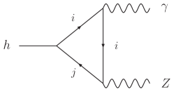
Figure 7: 1-loop contribution to $h\to Z\gamma$ from fermion species $i$ and $j$.

In the basis of mass eigenstates and focussing on fermions with the same electric charge, the terms of interest in the Lagrangian can be written in full generality as follows

$${\cal L}=\bar{\psi}^{i}\left(i\!\!\not\!\partial-m_{i}\right)\psi^{i}+\frac{1}{2}\bar{\psi}^{i}h\left(\lambda^{h}_{ij}+i\gamma^{5}\bar{\lambda}^{h}_{ij}\right)\psi^{j}+\frac{1}{2}\bar{\psi}^{i}Z_{\mu}\gamma^{\mu}\left(\lambda^{Z}_{ij}+\gamma_{5}\bar{\lambda}^{Z}_{ij}\right)\psi^{j}\,,$$ (F.1)

where a sum over all mass eigenstates $i,j$ is left understood and the matrices $\lambda^{h,Z}$, $\bar{\lambda}^{h,Z}$ are all hermitian. Possible derivative interactions of the Higgs with the fermions can always be rewritten as in Eq. (F.1) by integration by parts and use of the equations of motion. We will show this in detail in the following. By calculating the diagram of Fig. 7 and summing over $i,j$ one obtains the following decay amplitude

$$A_{NP}=-\frac{eQ_{\psi}}{4\pi^{2}}v\sum_{i,j}\left[\lambda^{h}_{ij}\lambda^{Z}_{ji}\,F(m_{i},m_{j},m_{h},m_{Z})+i\bar{\lambda}^{h}_{ij}\bar{\lambda}^{Z}_{ji}\,F(m_{i},-m_{j},m_{h},m_{Z})\right]\,.$$ (F.2)

The final result is thus obtained by further summing the contributions from fermions with different electric charge. The loop function is equal to [33]

$$\begin{split}F(m_{1},m_{2},m_{h},m_{Z})=\,&\frac{1}{2(m_{h}^{2}-m_{Z}^{2})}\,\times\\[4.26773pt] &\times\bigg{\{}\frac{m_{Z}^{2}(m_{1}+m_{2})}{(m_{h}^{2}-m_{Z}^{2})}\left[B_{0}(m_{Z}^{2},m_{1},m_{2})-B_{0}(m_{h}^{2},m_{1},m_{2})\right]\\[4.26773pt] &\hskip 24.18501pt+\bigg{[}-\frac{m_{1}}{2}(2m_{1}(m_{1}+m_{2})-m_{h}^{2}+m_{Z}^{2})C_{0}(m_{1},m_{1},m_{2})\\[4.26773pt] &\hskip 45.52458pt+(m_{1}\leftrightarrow m_{2})\bigg{]}-(m_{1}+m_{2})\bigg{\}}\,,\end{split}$$ (F.3)

where $B_{0}(p^{2},m_{1},m_{2}),C_{0}(p_{1}^{2},p_{2}^{2},(p_{1}+p_{2})^{2},m_{1},m_{2},m_{3})$ are two- and three-points Passarino-Veltman functions (for a review see Ref. [34]), and we define for convenience $C_{0}(m_{1},m_{2},m_{3})\equiv C_{0}(0,m_{Z}^{2},m_{h}^{2},m_{1},m_{2},m_{3})$. In the equal mass limit $m_{1}=m_{2}$ the loop function reduces to the SM one (see Eqs. (A.2), (A.4)):

$$F(m,m,m_{h},m_{Z})=\frac{1}{2m}(I_{1}(\tau_{f},\lambda_{f})-I_{2}(\tau_{f},\lambda_{f}))\,.$$ (F.4)

In the limit of heavy fermions, $m_{1}^{2},m_{2}^{2}\gg m_{h}^{2},m_{Z}^{2}$, the loop function reduces to

$$\begin{split}F(m_{1},m_{2},0,0)=\,&-\frac{1}{8\left(m_{1}-m_{2}\right)^{3}\left(m_{1}+m_{2}\right)^{2}}\,\times\\[4.26773pt] &\times\bigg{[}\left(m^{2}_{1}-m^{2}_{2}\right)\left(m_{1}^{2}-4m_{2}m_{1}+m_{2}^{2}\right)\\[4.26773pt] &\hskip 28.45274pt+4m_{1}m_{2}\left(m_{1}^{2}-m_{2}m_{1}+m_{2}^{2}\right)\log\!\left(\frac{m_{1}}{m_{2}}\right)\bigg{]}\,.\end{split}$$ (F.5)

If the Higgs is a NG boson, its interactions to the fermions can be only of derivative type, as shown for example in Eq. (E.1). In the mass-eigenstate basis the Lagrangian can thus be written as

$${\cal L}=\bar{\psi}^{i}\left(i\!\!\not\!\partial-m_{i}\right)\psi^{i}+\frac{1}{2}\bar{\psi}^{i}(\partial_{\mu}h)\gamma^{\mu}\left(T^{h}_{ij}+\gamma^{5}\bar{T}^{h}_{ij}\right)\psi^{j}+\frac{1}{2}\bar{\psi}^{i}Z_{\mu}\gamma^{\mu}\left(\lambda^{Z}_{ij}+\gamma_{5}\bar{\lambda}^{Z}_{ij}\right)\psi^{j}\,,$$ (F.6)

where $T^{h}$, $\bar{T}^{h}$ are hermitian. By integrating by parts and using the fermions’ equations of motion, the above Lagrangian can be re-written as:

$$\begin{split}{\cal L}=\,&\bar{\psi}^{i}\left(i\!\!\not\!\partial-m_{i}\right)\psi^{i}+\frac{1}{2}\bar{\psi}^{i}h\left[i(m_{j}-m_{i})T^{h}_{ij}+i\gamma^{5}(m_{i}+m_{j})\bar{T}^{h}_{ij}\right]\psi^{j}\\[2.84544pt] &+\frac{1}{2}\bar{\psi}^{i}Z_{\mu}\gamma^{\mu}\left(\lambda^{Z}_{ij}+\gamma_{5}\bar{\lambda}^{Z}_{ij}\right)\psi^{j}+O[(h^{2}\psi^{2}),(hZ\psi^{2})]\,.\end{split}$$ (F.7)

This is of the form (F.1) upon identifying

$$\lambda^{h}_{ij}=i(m_{j}-m_{i})T^{h}_{ij}\,,\qquad\bar{\lambda}^{h}_{ij}=(m_{i}+m_{j})\bar{T}^{h}_{ij}\,.$$ (F.8)

At the 1-loop level the $O(h^{2}\psi^{2})$ terms are irrelevant for $h\to Z\gamma$ and can be safely ignored. The $O(hZ\psi^{2})$ terms also do not contribute to $h\to Z\gamma$: they lead to (two-point like) diagrams whose loop function has a transverse Lorentz structure, $(q_{\mu}q_{\nu}-g_{\mu\nu}q^{2})$, where $q$ is the photon momentum, hence the corresponding Feynman amplitude vanishes identically for an on-shell photon. The final expression of the amplitude is thus given by Eq. (F.2), with $\lambda^{h}$ and $\bar{\lambda}^{h}$ given by Eq. (F.8).

In Section 3.2 we have computed the contribution to $h\to Z\gamma$ from pure composite fermions using an effective Lagrangian approach. For vanishing elementary-composite mixings, the composite multiplets of $SO(4)$ are mass eigenstates, and Eq. (E.1) is of the form (F.6) with $T^{h}\propto\zeta\,T^{\hat{4}}$ and $\bar{T}^{h}=0$. The vanishing of $\bar{T}^{h}$ follows from our tacit assumption to have the same coupling to the Higgs for both left- and right-handed chiralities of composite fermions in Eq. (E.1). By using the above results, in particular Eqs. (F.2), (F.8), and taking the limit of heavy fermion masses, the decay amplitude reads

$$A_{NP}=-\frac{eQ_{\psi}}{4\pi^{2}}\sum_{i,j}i(m_{j}-m_{i})T^{h}_{ij}\,\lambda^{Z}_{ji}\,F(m_{i},m_{j},0,0)\,.$$ (F.9)

By summing the contributions from mass eigenstates with different electric charge and using the identity

$$\frac{(m_{j}-m_{i})}{\pi^{2}}F(m_{i},m_{j},0,0)=C(m_{i},m_{j})-C(m_{j},m_{i})\,,$$ (F.10)

one finally re-obtains the result of Eq. (3.16).

References

- [1] ATLAS Collaboration, ATLAS-CONF-2013-034.
- [2] CMS Collaboration, CMS-PAS-HIG-13-005.
- [3] C. J. C. Burges and H. J. Schnitzer, Nucl. Phys. B 228 (1983) 464; C. N. Leung, S. T. Love and S. Rao, Z. Phys. C 31 (1986) 433; W. Buchmuller and D. Wyler, Nucl. Phys. B 268 (1986) 621.
- [4] R. Rattazzi, Z. Phys. C 40 (1988) 605; B. Grzadkowski, Z. Hioki, K. Ohkuma and J. Wudka, Nucl. Phys. B 689 (2004) 108 [hep-ph/0310159]; P. J. Fox, Z. Ligeti, M. Papucci, G. Perez and M. D. Schwartz, Phys. Rev. D 78 (2008) 054008 [arXiv:0704.1482 [hep-ph]]; J. A. Aguilar-Saavedra, Nucl. Phys. B 812 (2009) 181 [arXiv:0811.3842 [hep-ph]]; J. A. Aguilar-Saavedra, Nucl. Phys. B 821 (2009) 215 [arXiv:0904.2387 [hep-ph]]; C. Grojean, W. Skiba and J. Terning, Phys. Rev. D 73 (2006) 075008 [hep-ph/0602154].
- [5] B. Grzadkowski, M. Iskrzynski, M. Misiak and J. Rosiek, JHEP 1010 (2010) 085 [arXiv:1008.4884 [hep-ph]].
- [6] R. Contino, M. Ghezzi, C. Grojean, M. Muhlleitner and M. Spira, JHEP 1307 (2013) 035 [arXiv:1303.3876 [hep-ph]].
- [7] G. F. Giudice, C. Grojean, A. Pomarol, R. Rattazzi, JHEP 0706 (2007) 045, [arXiv:hep-ph/0703164].
- [8] M. E. Peskin and T. Takeuchi, Phys. Rev. D 46 (1992) 381; R. Barbieri, A. Pomarol, R. Rattazzi, A. Strumia, Nucl. Phys. B703 (2004) 127-146, [arXiv:hep-ph/0405040].
- [9] E. E. Jenkins, A. V. Manohar and M. Trott, arXiv:1305.0017 [hep-ph].
- [10] R. Contino, D. Marzocca, D. Pappadopulo and R. Rattazzi, JHEP 1110 (2011) 081 [arXiv:1109.1570 [hep-ph]].
- [11] S. R. Coleman, J. Wess, B. Zumino, Phys. Rev. 177 (1969) 2239-2247. C. G. Callan, Jr., S. R. Coleman, J. Wess et al., Phys. Rev. 177 (1969) 2247-2250.
- [12] C. Grojean, E. E. Jenkins, A. V. Manohar and M. Trott, JHEP 1304 (2013) 016 [arXiv:1301.2588 [hep-ph]].
- [13] J. Elias-Miro, J. R. Espinosa, E. Masso and A. Pomarol, arXiv:1302.5661 [hep-ph].
- [14] K. Agashe, R. Contino, L. Da Rold and A. Pomarol, Phys. Lett. B 641 (2006) 62 [hep-ph/0605341].
- [15] J. Mrazek, A. Pomarol, R. Rattazzi, M. Redi, J. Serra and A. Wulzer, Nucl. Phys. B 853 (2011) 1 [arXiv:1105.5403 [hep-ph]].
- [16] R. Contino, L. Da Rold and A. Pomarol, Phys. Rev. D 75 (2007) 055014 [hep-ph/0612048].
- [17] R. Contino, T. Kramer, M. Son and R. Sundrum, JHEP 0705 (2007) 074 [hep-ph/0612180].
- [18] D. B. Kaplan, Nucl. Phys. B 365 (1991) 259.
- [19] H. Cai, arXiv:1306.3922 [hep-ph].
- [20] A. Orgogozo and S. Rychkov, JHEP 1306 (2013) 014 [arXiv:1211.5543 [hep-ph]].
- [21] G. Ecker, J. Gasser, H. Leutwyler, A. Pich and E. de Rafael, Phys. Lett. B 223 (1989) 425.
- [22] M. Golden and L. Randall, Nucl. Phys. B 361 (1991) 3.
- [23] R. Barbieri, G. Isidori and D. Pappadopulo, JHEP 0902 (2009) 029 [arXiv:0811.2888 [hep-ph]].
- [24] C. Grojean, O. Matsedonskyi and G. Panico, arXiv:1306.4655 [hep-ph].
- [25] G. Panico and A. Wulzer, JHEP 0705 (2007) 060 [hep-th/0703287].
- [26] M. S. Carena, E. Ponton, J. Santiago and C. E. M. Wagner, Nucl. Phys. B 759 (2006) 202 [hep-ph/0607106]; Phys. Rev. D 76 (2007) 035006 [hep-ph/0701055]; G. Panico, M. Safari and M. Serone, JHEP 1102 (2011) 103 [arXiv:1012.2875 [hep-ph]].
- [27] G. Panico, M. Redi, A. Tesi and A. Wulzer, JHEP 1303 (2013) 051 [arXiv:1210.7114 [hep-ph]].
- [28] A. De Simone, O. Matsedonskyi, R. Rattazzi and A. Wulzer, JHEP 1304 (2013) 004 [arXiv:1211.5663 [hep-ph]].
- [29] M. Baak, M. Goebel, J. Haller, A. Hoecker, D. Kennedy, R. Kogler, K. Moenig and M. Schott et al., Eur. Phys. J. C 72 (2012) 2205 [arXiv:1209.2716 [hep-ph]].
- [30] M. Ciuchini, E. Franco, S. Mishima and L. Silvestrini, arXiv:1306.4644 [hep-ph].
- [31] A. Pomarol and J. Serra, Phys. Rev. D 78 (2008) 074026 [arXiv:0806.3247 [hep-ph]].
- [32] A. Falkowski, F. Riva and A. Urbano, arXiv:1303.1812 [hep-ph].
- [33] A. Djouadi, V. Driesen, W. Hollik and A. Kraft, Eur. Phys. J. C 1, 163 (1998) [hep-ph/9701342].
- [34] D. Y. Bardin and G. Passarino, “The standard model in the making: Precision study of the electroweak interactions” (International series of monographs on physics. 104).