Adaptive and Iterative Multi-Branch MMSE Decision Feedback Detection Algorithms for MIMO Systems

Abstract

In this work, decision feedback (DF) detection algorithms based on multiple processing branches for multi-input multi-output (MIMO) spatial multiplexing systems are proposed. The proposed detector employs multiple cancellation branches with receive filters that are obtained from a common matrix inverse and achieves a performance close to the maximum likelihood detector (MLD). Constrained minimum mean-squared error (MMSE) receive filters designed with constraints on the shape and magnitude of the feedback filters for the multi-branch MMSE DF (MB-MMSE-DF) receivers are presented. An adaptive implementation of the proposed MB-MMSE-DF detector is developed along with a recursive least squares-type algorithm for estimating the parameters of the receive filters when the channel is time-varying. A soft-output version of the MB-MMSE-DF detector is also proposed as a component of an iterative detection and decoding receiver structure. A computational complexity analysis shows that the MB-MMSE-DF detector does not require a significant additional complexity over the conventional MMSE-DF detector, whereas a diversity analysis discusses the diversity order achieved by the MB-MMSE-DF detector. Simulation results show that the MB-MMSE-DF detector achieves a performance superior to existing suboptimal detectors and close to the MLD, while requiring significantly lower complexity.

I Introduction

The deployment of multiple transmit and receive antennas in wireless communication systems can offer significant multiplexing [1, 2] and diversity gains [3, 4]. The multiplexing gains enable high spectral efficiencies, whereas the diversity gains increase the reliability of the links and provide low error rates. In multi-input multi-output (MIMO) systems, the transmitter and the receiver should be appropriately designed in order to exploit the structure of the propagation channels. In a spatial multiplexing configuration, the capacity gain grows linearly with the minimum number of transmit and receive antennas [1, 2]. In this scenario, the system can obtain substantial gains in data rate with the transmission of individual data streams from the transmitter to the receiver. In order to separate these streams, a designer must resort to MIMO detection techniques, which are similar to multiuser detection methods [5]. The optimal maximum likelihood (ML) detector is too complex to be implemented in systems with a large number of antennas. The ML solution can be alternatively computed using sphere decoder (SD) algorithms [6]-[12], which are very efficient for MIMO systems with a small number of antennas. However, the computational complexity of SD algorithms depends on the noise variance, the number of data streams to be detected and the signal constellation, resulting in high computational costs for low signal-to-noise ratios (SNR), large MIMO systems and high-order constellations. The high computational complexity of the ML detector and the SD algorithms in some of the aforementioned situations have motivated the development of numerous alternative strategies for MIMO detection. The linear detector [13], the successive interference cancellation (SIC) approach used in the Vertical-Bell Laboratories Layered Space-Time (VBLAST) systems [15]-[17] and other decision-driven detectors such as decision feedback (DF) [18]-[61] are techniques that can offer attractive trade-offs between performance and complexity. Prior work on DF schemes has been reported with DF detectors with SIC (S-DF) [18, 61, 29] and DF receivers with parallel interference cancellation (PIC) (P-DF) [32, 33], combinations of these schemes [32, 35, 36, 38] and mechanisms to mitigate error propagation [39, 40]. An often criticized aspect of these sub-optimal schemes is that they typically do not achieve the full receive-diversity order of the ML algorithm. This has motivated the investigation of alternative detection strategies such as lattice-reduction (LR) schemes [23]-[24], QR decomposition and the M-algorithm (QRD-M) detectors [25, 26] , probabilistic data association (PDA) [27, 28] detectors, extensions to soft-input soft-output detectors [58]-[62], and calls for flexible cost-effective detection algorithms with near-ML or ML performance, which achieve the full receive-diversity order.

In this work, a DF detection strategy based on multiple branches (MB) is proposed for MIMO systems operating in a spatial multiplexing configuration. The proposed detection algorithm, termed as MB-MMSE-DF and first reported in [37], employs multiple feedforward and feedback receive filters with appropriate transformations that are obtained from a common matrix inverse and allow the search for improved detection candidates. To this end, the MB-MMSE-DF receiver exploits different patterns and orderings, and selects the branch with the highest likelihood based on an instantaneous MMSE metric. Constrained minimum mean-squared error (MMSE) receive filters designed with constraints on the shape and magnitude of the feedback filters for the proposed MB-MMSE-DF receiver are devised. The MB-MMSE-DF detector does not require a significant additional complexity over the conventional MMSE-DF receiver since it relies on filter realizations with different constraints on the feedback filters, a common matrix inversion and the same second-order statistics. An adaptive implementation of the MB-MMSE-DF detector with a recursive least squares (RLS)-type algorithm for estimating the parameters of the filters when the channel is time-varying is also presented. The optimal ordering algorithm for the MB-MMSE-DF detector is presented along with a low-complexity suboptimal ordering technique. A soft-input soft-output version of the MB-MMSE-DF receiver for iterative detection and decoding using convolutional codes is also developed. The iterative MB-MMSE-DF receiver employs multiple detection candidates to construct a list of log-likelihood ratios for each transmitted bit. A diversity analysis that discusses the diversity order achieved by the MB-MMSE-DF detector is carried out along with a computational complexity study. The MB-MMSE-DF detector achieves a performance close to the optimal ML detector, while it requires a reduced cost and has a superior performance to existing sub-optimal detectors.

The main contributions of this work are:
1) The proposal of the MB-MMSE-DF detection algorithm;
2) MMSE expressions for filter design along with shape patterns and magnitude constraints for the filters;
3) An adaptive version of the proposed detection scheme along with a performance and a complexity analysis;
4) An optimal ordering algorithm is presented along with a cost-effective suboptimal ordering algorithm for the MB-MMSE-DF detector;
5) An iterative MB-MMSE-DF algorithm for processing soft estimates with convolutional codes;
6) An analysis of the complexity and diversity order attained by the MB-MMSE-DF detector;
7) A comparative study of the MB-MMSE-DF and existing MIMO detection algorithms.

This paper is organized as follows. Section II briefly describes a MIMO spatial multiplexing system model. Section III is devoted to the proposed MB-MMSE-DF detection algorithm, the design of the MMSE filters and a multistage scheme. Section IV presents the design of the shaping matrices, the ordering and the parameter estimation algorithms. Section V is dedicated to the development of an iterative version of the MB-MMSE-DF detector which processes soft information for iterative detection and decoding. Section VI presents an analysis of the computational complexity along with the diversity order of the MB-MMSE-DF scheme. Section VII presents and discusses the simulation results and Section VIII draws the conclusions.

II System Model

Consider a spatial multiplexing MIMO system with $N_{T}$ transmit antennas and $N_{R}$ receive antennas, where $N_{R}\geq N_{T}$. At each time instant $i$, the system transmits $N_{T}$ symbols which are organized into a $N_{T}\times 1$ vector ${\boldsymbol{s}}[i]=\big{[}s_{1}[i],~{}s_{2}[i],~{}\ldots,~{}s_{N_{T}}[i]\big{]}^{T}$ taken from a modulation constellation $A=\{a_{1},~{}a_{2},~{}\ldots,~{}a_{N}\}$, where $(\cdot)^{T}$ denotes transpose and $N=2^{C}$. In other words, each symbol is carrying $C$ bits. The symbol vector ${\boldsymbol{s}}[i]$ is then transmitted over flat fading channels and the signals are demodulated and sampled at the receiver, which is equipped with $N_{R}$ antennas.

The received signal after demodulation, matched filtering and sampling is organized in an $N_{R}\times 1$ vector ${\boldsymbol{r}}[i]=\big{[}r_{1}[i],~{}r_{2}[i],~{}\ldots,~{}r_{N_{R}}[i]\big{]}^{T}$ with sufficient statistics for detection as given by

$${\boldsymbol{r}}[i]={\boldsymbol{H}}{\boldsymbol{s}}[i]+{\boldsymbol{n}}[i],$$ (1)

where the $N_{R}\times 1$ vector ${\boldsymbol{n}}[i]$ is a zero mean complex circular symmetric Gaussian noise with covariance matrix $E\big{[}{\boldsymbol{n}}[i]{\boldsymbol{n}}^{H}[i]\big{]}=\sigma_{n}^{2}{\boldsymbol{I}}$, where $E[\cdot]$ stands for expected value, $(\cdot)^{H}$ denotes the Hermitian operator, $\sigma_{n}^{2}$ is the noise variance and ${\boldsymbol{I}}$ is the identity matrix. The symbol vector ${\boldsymbol{s}}[i]$ has zero mean and a covariance matrix $E\big{[}{\boldsymbol{s}}[i]{\boldsymbol{s}}^{H}[i]\big{]}=\sigma_{s}^{2}{\boldsymbol{I}}$, where $\sigma_{s}^{2}$ is the signal power. The elements $h_{n_{R},n_{T}}$ of the $N_{R}\times N_{T}$ channel matrix ${\boldsymbol{H}}$ correspond to the complex channel gains from the $n_{T}$th transmit antenna to the $n_{R}$th receive antenna.

III Multi-Branch MMSE Decision Feedback Detection

Figure 1: Block diagram of the proposed MB-MMSE-DF detector and the processing of the $j$th data stream.

In this section, the structure of the proposed MB-MMSE-DF detector for MIMO systems is presented and a schematic of the detector is shown in Fig. 1. The MB-MMSE-DF detector employs multiple pairs of MMSE receive filters in such a way that the detector can obtain different local maxima of the likelihood function and select the best candidate for detection according to an instantaneous MMSE metric for each received data symbol. The receive filters are designed based on the MMSE statistical criterion whereas the detection and the selection of the best candidate for each received symbol relies on an instantaneous MMSE criterion. The MB-MMSE-DF scheme is flexible and approaches the full receive diversity available in the system by increasing the number of branches. The MB-MMSE-DF detector employs tasks such as MB processing, MMSE decision feedback, and ordering that have a combined computational cost that is substantially lower than the ML detector, which is very simple from a mathematical point of view but requires a number of operations that is much higher than the MB-MMSE-DF and other existing detectors.

In order to detect each transmitted data stream using the proposed MB-MMSE-DF detector, the receiver linearly combines the feedforward filter represented by the $N_{R}\times 1$ vector ${\boldsymbol{w}}_{j,l}$ corresponding to the $j$-th data stream and the $l$-th branch with the received vector ${\boldsymbol{r}}[i]$, subtracts the remaining interference by linearly combining the feedback filter denoted by the $N_{T}\times 1$ vector ${\boldsymbol{f}}_{j,l}$ with the $N_{T}\times 1$ vector of initial decisions $\hat{\boldsymbol{s}}_{l}[i]$ obtained from previous decisions. This process is repeated for $L$ candidate symbols and $N_{T}$ data streams as described by

$$\begin{split}{z}_{j,l}[i]&={\boldsymbol{w}}^{H}_{j,l}{\boldsymbol{r}}[i]-{\boldsymbol{f}}_{j,l}^{H}\hat{\boldsymbol{s}}_{l}[i],~{}~{}j=1,~{}\ldots,~{}N_{T}~{}~{}{\rm and}~{}~{}l=1,~{}\ldots,~{}L\end{split}$$ (2)

where the input to the decision device for the $i$th symbol and the $j$-th stream is the $L\times 1$ vector ${\boldsymbol{z}}_{j}[i]=[z_{j,1}[i]~{}\ldots~{}z_{j,L}[i]]^{T}$. The number of parallel branches $L$ that produce detection candidates is a parameter that must be chosen by the designer and is determined experimentally. Another important design aspect that affects the performance is the ordering algorithm which will be discussed later on. The goal of this work is to employ a reduced number of branches and yet achieve near-ML or ML performance.

The MB-MMSE-DF detector generates $L$ candidate symbols for each data stream and then selects the best branch according to an instantaneous MMSE metric as described by

$$l_{j,{\rm opt}}=\arg\min_{1\leq l_{j}\leq L}{\rm IMMSE}(s_{j}[i],{\boldsymbol{w}}_{j,l},{\boldsymbol{f}}_{j,l},{\boldsymbol{r}}[i]),~{}j=1,~{}\ldots,~{}N_{T}$$ (3)

where

$${\rm IMMSE}(s_{j}[i],{\boldsymbol{w}}_{j,l},{\boldsymbol{f}}_{j,l},{\boldsymbol{r}}[i])\approx|s_{j}[i]|^{2}-{\boldsymbol{w}}_{j,l}^{H}\hat{\boldsymbol{R}}[i]{\boldsymbol{w}}_{j,l}+{\boldsymbol{f}}_{j,l}^{H}\hat{\boldsymbol{s}}_{l}[i]\hat{\boldsymbol{s}}^{H}_{l}[i]{\boldsymbol{f}}_{j,l}$$ (4)

where the instantaneous MMSE metric IMMSE is produced by the pair of receive filters ${\boldsymbol{w}}_{j,l}$ and ${\boldsymbol{f}}_{j,l}$, the quantity $|s_{j}[i]|^{2}$, the received vector ${\boldsymbol{r}}[i]$ and an instantaneous estimate of the covariance matrix $\hat{\boldsymbol{R}}[i]={\boldsymbol{r}}[i]{\boldsymbol{r}}^{H}[i]$. Further details about the MMSE and IMMSE expressions are included in the Appendices.

The final detected symbol of the MB-MMSE-DF detector is obtained by using the best branch as given by

$$\begin{split}\hat{s}_{j}[i]&=Q\big{[}{\boldsymbol{z}}_{j,l_{j,{\rm opt}}}[i]\big{]}=Q\big{[}{\boldsymbol{w}}^{H}_{j,l_{j,{\rm opt}}}{\boldsymbol{r}}[i]-{\boldsymbol{f}}_{j,l_{j,{\rm opt}}}^{H}\hat{\boldsymbol{s}}_{l_{j,{\rm opt}}}[i]\big{]},~{}j=1,~{}\ldots,~{}N_{T}\end{split}$$ (5)

where $Q(\cdot)$ is a slicing function that makes the decisions about the symbols, which can be drawn from an M-PSK or a QAM constellation.

III-A MMSE Filter Design

In this part, the design of the MMSE receive filters of the proposed MB-MMSE-DF detector is detailed by first assuming imperfect feedback of the symbol decisions (${\boldsymbol{s}}\neq\hat{\boldsymbol{s}}$) and then by assuming perfect feedback (${\boldsymbol{s}}=\hat{\boldsymbol{s}}$). The design of the receive filters is equivalent to determining feedforward filters ${\boldsymbol{w}}_{j,l}$ with $N_{R}$ coefficients and feedback filters ${\boldsymbol{f}}_{j,l}$ with $N_{T}$ elements subject to certain shape constraints on ${\boldsymbol{f}}_{j,l}$ in accordance to the following optimization problem

$$\begin{split}{\rm min}&~{}{\rm MSE}(s_{j}[i],{\boldsymbol{w}}_{j,l},{\boldsymbol{f}}_{j,l})=E\big{[}|{s}_{j}[i]-{\boldsymbol{w}}^{H}_{j,l}{\boldsymbol{r}}[i]+{\boldsymbol{f}}_{j,l}^{H}\hat{\boldsymbol{s}}_{l}[i]|^{2}\big{]}\\ &{\rm subject}~{}{\rm to}~{}{\boldsymbol{S}}_{j,l}{\boldsymbol{f}}_{j,l}={\boldsymbol{0}}~{}~{}{\rm and}~{}~{}||{\boldsymbol{f}}_{j,l}||^{2}=\gamma_{j,l}||{\boldsymbol{f}}_{j,l}^{c}||^{2},{\rm for}~{}j=1,\ldots,N_{T}~{}{\rm and}~{}l=1,\ldots,L,\end{split}$$ (6)

where the $N_{T}\times N_{T}$ shape constraint matrix is ${\boldsymbol{S}}_{j,l}$, ${\boldsymbol{0}}$ is a $N_{T}\times 1$ constraint vector and $\gamma_{j,l}$ is a design parameter that ranges from $0$ to $1$ and is responsible for scaling the norm of the conventional feedback receive filter ${\boldsymbol{f}}_{j,l}^{c}$. The scaling of ${\boldsymbol{f}}_{j,l}^{c}$ results in the desired feedback receive filter ${\boldsymbol{f}}_{j,l}$. The expectation operator is taken over the random parameters ${\boldsymbol{s}}[i]$ and ${\boldsymbol{r}}[i]$ assuming that ${\boldsymbol{n}}[i]$ and ${\boldsymbol{s}}[i]$ are statistically independent, and that the entries of ${\boldsymbol{s}}[i]$ and ${\boldsymbol{n}}[i]$ are independent and identically distributed random variables. The role of the shape constraint matrix ${\boldsymbol{S}}_{j,l}$ is to choose the feedback connections which will be used in the interference cancellation. If a designer employs multiple branches and shape constraint matrices along with different orderings then multiple candidates for detection can be generated, resulting in an improved receiver performance. The rationale for scaling the norm of the feedback filter is to reduce the impact of the error propagation and improve the performance of the receiver. This is accomplished by judiciously adjusting the scaling of the norm and employing the value which minimizes the error propagation.

In what follows, the optimal MMSE receive filters based on the proposed optimization in (6) are derived. By resorting to the method of Lagrange multipliers, computing the gradient vectors of the Lagrangian with respect to ${\boldsymbol{w}}_{j,l}$ and ${\boldsymbol{f}}_{j,l}$, equating them to null vectors and rearranging the terms, we obtain ${\rm for}~{}j=1,\ldots,N_{T}$ and $l=1,\ldots,L$

$${\boldsymbol{w}}_{j,l}^{\rm MMSE}={\boldsymbol{R}}^{-1}({\boldsymbol{p}}_{j}+{\boldsymbol{Q}}{\boldsymbol{f}}_{j,l}),$$ (7)

$$\begin{split}{\boldsymbol{f}}_{j,l}^{\rm MMSE}&=\frac{\beta_{j,l}}{\sigma_{s}^{2}}{\boldsymbol{\Pi}}_{j,l}({\boldsymbol{Q}}^{H}{\boldsymbol{w}}_{j,l}-{\boldsymbol{t}}_{j}),\end{split}$$ (8)

where

$${\boldsymbol{\Pi}}_{j,l}={\boldsymbol{I}}-{\boldsymbol{S}}_{j,l}^{H}({\boldsymbol{S}}_{j,l}^{H}{\boldsymbol{S}}_{j,l})^{-1}{\boldsymbol{S}}_{j,l}$$ (9)

is a projection matrix that ensures the shape constraint ${\boldsymbol{S}}_{j,l}$ on the feedback filter, $\beta_{j,l}=(1-\mu_{j,l})^{-1}$ is the parameter that controls the ability of the MB-MMSE-DF detector to mitigate error propagation with values $0\leq\beta_{j,l}\leq 1$, and $\mu_{j,l}$ is the Lagrange multiplier. It should be remarked that the inverse $({\boldsymbol{S}}_{j,l}^{H}{\boldsymbol{S}}_{j,l})^{-1}$ might not exist. In these situations, a pseudo-inverse is computed. The relationship between $\beta_{j,l}$ and $\gamma_{j,l}$ is not in closed-form except for the extreme values when we have $\beta_{j,l}=0$ and $\beta_{j,l}=1$ for $\gamma_{j,l}=0$ (standard linear MMSE detector) and $\gamma_{j,l}=1$ ( standard MB-MMSE-DF detector), respectively. The optimization of the parameter $\beta_{j,l}$ has been done with the aid of simulations because there is no closed-form solution to obtain $\beta_{j,l}$. The simulation approach has indicated that the performance is improved for a range of parameters between $0.6$ and $0.7$. This range of parameters was verified to consistently produce good results for all the scenarios investigated with the MB-MMSE-DF detector. The $N_{R}\times N_{R}$ covariance matrix of the input data vector is ${\boldsymbol{R}}=E[{\boldsymbol{r}}[i]{\boldsymbol{r}}^{H}[i]]$, ${\boldsymbol{p}}_{j}=E[{\boldsymbol{r}}[i]s_{j}^{*}[i]]$, ${\boldsymbol{Q}}=E\big{[}{\boldsymbol{r}}[i]\hat{\boldsymbol{s}}_{l}^{H}[i]\big{]}$, and ${\boldsymbol{t}}_{j}=E[\hat{\boldsymbol{s}}_{l}[i]{s}_{j}^{*}[i]]$ is the $N_{T}\times 1$ vector of correlations between $\hat{\boldsymbol{s}}_{l}[i]$ and ${s}_{j}^{*}[i]$. Substituting (8) into (7) and then further manipulating the expressions we arrive at the following MMSE receive filter expressions

$${\boldsymbol{w}}_{j,l}^{\rm MMSE}=\big{(}{\boldsymbol{R}}-\beta_{j,l}{\boldsymbol{Q}}{\boldsymbol{\Pi}}_{j,l}{\boldsymbol{Q}}^{H}\big{)}^{-1}\big{(}{\boldsymbol{p}}_{j}-\beta_{j,l}{\boldsymbol{\Pi}}_{j,l}{\boldsymbol{t}}_{j}\big{)},$$ (10)

$$\begin{split}{\boldsymbol{f}}_{j,l}^{\rm MMSE}&=\frac{\beta_{j,l}}{\sigma_{s}^{2}}{\boldsymbol{\Pi}}_{j,l}\big{(}{\boldsymbol{Q}}^{H}\big{(}{\boldsymbol{R}}-\beta_{j,l}{\boldsymbol{Q}}{\boldsymbol{\Pi}}_{j,l}{\boldsymbol{Q}}^{H}\big{)}^{-1}\big{(}{\boldsymbol{p}}_{j}-\beta_{j,l}{\boldsymbol{Q}}{\boldsymbol{\Pi}}_{j,l}{\boldsymbol{t}}_{j}\big{)}-{\boldsymbol{t}}_{j}).\end{split}$$ (11)

The above expressions only depend on statistical quantities, and consequently on the channel matrix ${\boldsymbol{H}}$, the symbol and noise variances $\sigma^{2}_{s}$ and $\sigma^{2}_{n}$, respectively, and the constraints. However, the matrix inversion required for computing ${\boldsymbol{w}}_{j,l}$ is different for each branch and data stream, thereby rendering the scheme computationally less efficient. The expressions obtained in (7) and (8) are equivalent to those in (10) and (11), and only require iterations between them for an equivalent performance. A key advantage of using (7) and (8) is that they only require a single matrix inversion that is common to all branches and two iterations prior to their use, whereas in (10) and (11) there is a matrix inversion associated with each branch. For this reason, in what follows the expressions in (7) and (8) are adopted and further simplified.

As briefly explained above, the expressions in (7) and (8) can be simplified by evaluating the expected values. By using the fact that ${\boldsymbol{t}}_{j}={\boldsymbol{0}}$ for interference cancellation as $\hat{\boldsymbol{s}}_{l}[i]$ does not contain $s_{j}$ and assuming perfect feedback (${\boldsymbol{s}}=\hat{\boldsymbol{s}}$), the following expressions are obtained

$${\boldsymbol{w}}_{j,l}^{\rm MMSE}=\big{(}{\boldsymbol{H}}{\boldsymbol{H}}^{H}+{\sigma_{n}^{2}}/{\sigma_{s}^{2}}{\boldsymbol{I}}\big{)}^{-1}{\boldsymbol{H}}({\boldsymbol{\delta}}_{j}+{\boldsymbol{f}}_{j,l}),$$ (12)

$${\boldsymbol{f}}_{j,l}^{\rm MMSE}=\beta_{j,l}{\boldsymbol{\Pi}}_{j,l}{\boldsymbol{H}}^{H}{\boldsymbol{w}}_{j,l},$$ (13)

where ${\boldsymbol{\delta}}_{j}=[\underbrace{0\ldots 0}_{j-1}~{}1~{}\underbrace{0\ldots 0}_{N_{T}-j-2}]^{T}$ is a $N_{T}\times 1$ vector with a one in the $j$th element and zeros elsewhere. A step-by-step derivation of the filters is shown in Appendix I. The proposed MB-MMSE-DF detector expressions above require the channel matrix ${\boldsymbol{H}}$ (in practice an estimate of it) and the noise variance $\sigma_{n}^{2}$ at the receiver. In terms of complexity, it requires for each branch $l$ the inversion of an $N_{R}\times N_{R}$ matrix and other operations with complexity $O(N_{R}^{3})$. However, the expressions obtained in (7) and (8) for the general case, and in (12) and (13) for the case of perfect feedback, reveal that the most expensive operations, i.e., the matrix inversions, are identical for all branches. Therefore, the design of receive filters for the multiple branches only requires further additions and multiplications of the matrices. Moreover, it can be verified that the filters ${\boldsymbol{w}}_{j,l}^{\rm MMSE}$ and ${\boldsymbol{f}}_{j,l}^{\rm MMSE}$ are dependent on one another, which means the designer has to iterate them before applying the detector. It has been verified by simulations with different system parameters and by comparing the resulting parameters of the receive filters with those obtained by (10) and (11) that it suffices to employ two iterations of (12) and (13) to have a performance equivalent to that obtained by using (10) and (11). For this reason, we employ the receive filters of (12) and (13) with two iterations in the proposed MB-MMSE-DF detector.

The MMSE associated with the filters ${\boldsymbol{w}}_{j,l}^{\rm MMSE}$ and ${\boldsymbol{f}}_{j,l}^{\rm MMSE}$ and the statistics of the data symbols $s_{j}[i]$ is given by

$$\begin{split}\underbrace{{\rm MMSE}(s_{j}[i],{\boldsymbol{w}}_{j,l}^{\rm MMSE},{\boldsymbol{f}}_{j,l}^{\rm MMSE})}_{{\rm MMSE}_{j}}&=\sigma_{s}^{2}-{\boldsymbol{w}}_{j,l}^{H,~{}{\rm MMSE}}{\boldsymbol{R}}{\boldsymbol{w}}_{j,l}^{\rm MMSE}+{\boldsymbol{f}}_{j,l}^{H,~{}{\rm MMSE}}{\boldsymbol{f}}_{j,l}^{\rm MMSE},\end{split}$$ (14)

where $\sigma_{s}^{2}=E[|s_{j}[i]|^{2}]$ is the variance of the desired symbol. A detailed derivation of the MMSE associated with the receive filters is shown in Appendix II along with connections with the MMSE achieved by conventional DF detectors.

III-B Multi-stage Detection for the MB-MMSE-DF

In this subsection, algorithms for error propagation mitigation are presented and incorporated into the structure of the MB-MMSE-DF detection scheme. The strategy is based on iterative multi-stage detection [32, 35] that gradually refines the decision vector and improves the overall performance. It is incorporated into the MB-MMSE-DF scheme and the improvements in the detection performance are then investigated.

Figure 2: Block diagram of the proposed two-stage MB-MMSE-DF detector.

The basic principle underlying multi-stage detection is to iteratively refine the estimates of the decision vector used in DF receivers [32, 35] and mitigate error propagation. An advantage of multi-stage detection that has not been exploited for the design of MIMO detectors is that of equalizing the performance of the detectors over the data streams. Since V-BLAST or DF detection usually favors certain data streams (the last detected ones) with respect to performance, this might be important for some applications where fairness or uniform performance is required between the data streams. This concept is incorporated into the proposed MB-MMSE-DF scheme and the MMSE design of the previous subsection. An MB-MMSE-DF scheme is employed in each stage and the estimates of the decision vector are gradually refined as illustrated in Fig. 2. Specifically, a multi-stage algorithm for the MB-MMSE-DF can be described by

$${z}^{(m+1)}_{j,l}(i)={\boldsymbol{w}}_{j,l}^{H,~{}\rm MMSE}{\boldsymbol{r}}[i]-{\boldsymbol{f}}_{j,l}^{H,~{}{\rm MMSE}}\hat{\boldsymbol{s}}^{(m)}_{l}[i],~{}~{}m=0,~{}1,~{}\ldots,~{}M,$$ (15)

where the MMSE filters ${\boldsymbol{w}}_{j,l}^{\rm MMSE}$ and ${\boldsymbol{f}}_{j,l}^{\rm MMSE}$ are designed with the approach detailed in the previous subsection, $M$ denotes the number of stages and $\hat{\boldsymbol{s}}^{(m)}_{l}[i]$ is the vector of tentative decisions from the preceding iteration that is described by

$$\hat{s}^{(0)}_{j,l}[i]={\rm Q}\Big{(}{\boldsymbol{w}}_{j,l}^{H,~{}\rm MMSE}{\boldsymbol{r}}[i]\Big{)},~{}~{}j,l=1,~{}\ldots,~{}N_{T},$$ (16)

$$\hat{s}^{(m)}_{j,l_{j,{\rm opt}}}[i]={\rm Q}\Big{(}z^{(m)}_{j,l_{j,{\rm opt}}}[i]\Big{)},~{}m=1,~{}\ldots,~{}M,$$ (17)

where the number of stages $M$ depends on the scenario.

In order to equalize the performance over the data streams, an M-stage structure is considered. The first stage is an MB-MMSE-DF scheme with filters ${\boldsymbol{w}}_{j,l}^{\rm MMSE}$ and ${\boldsymbol{f}}_{j,l}^{\rm MMSE}$. The tentative decisions are passed to the second stage, which consists of another MB-MMSE-DF scheme with the same receive filters that uses the decisions of the first stage and so successively. The resulting multi-stage MIMO detection scheme is denoted I-MB-MMSE-DF. The output of the second stage of the resulting scheme is

$$z_{j,l}^{(2)}[i]=[{\boldsymbol{T}}{\boldsymbol{w}}_{j,l}^{\rm MMSE}]^{H}{\boldsymbol{r}}[i]-[{\boldsymbol{T}}{\boldsymbol{f}}_{j,l}^{\rm MMSE}]^{H}\hat{\boldsymbol{s}}^{(1)}_{l_{j,{\rm opt}}}[i],$$ (18)

where $z_{j,l}^{(2)}[i]$ is the output of $j$th data stream after multi-stage detection with $M=2$ stages, ${\boldsymbol{T}}$ is a square permutation matrix with ones along the reverse diagonal and zeros elsewhere. When multiple stages are used, it is beneficial to demodulate the data streams successively and in reverse order relative to the first branch of the MB-MMSE-DF detector. The role of reversing the cancellation order in successive stages is to equalize the performance of the users over the population or at least reduce the performance disparities. It provides a better performance than keeping the same ordering as the last decoded users in the first stage tend to be favored by the reduced interference. The rationale is that the performance can be improved by using the data streams that benefited from interference cancellation (last decoded ones) as the first ones to be decoded in the second stage. Additional stages can be included, although the results suggest that the gains in performance are marginal for more than two stages. Hence, the two-stage scheme is adopted for the rest of this work.

IV Design of Cancellation Patterns, Ordering and Adaptive Algorithms

In this section, the design of the shape constraint matrices ${\boldsymbol{S}}_{j,l}$ is detailed and their choices are motivated. An optimal and a suboptimal ordering algorithms are described for the interference cancellation. An adaptive version of the MB-MMSE-DF detector with RLS-type algorithms is also devised.

IV-A Design of Cancellation Patterns

The idea of the shape constraint matrices ${\boldsymbol{S}}_{j,l}$ is to modify the structure of the feedback filters ${\boldsymbol{f}}_{j,l}$ in such a way that only the selected feedback elements of ${\boldsymbol{f}}_{j,l}$ will be used to cancel the interference between the data streams. The feedback connections perform interference cancellation with a chosen ordering. If a designer employs multiple branches and shape constraint matrices along with different orderings then multiple candidates for detection can be generated, resulting in an improved receiver performance. The matrices ${\boldsymbol{S}}_{j,l}$ for the $N_{T}$ data streams and for the $L$ branches of the MB-MMSE-DF detector can be stored at the receiver and used either online or offline in the design of the feedback filters ${\boldsymbol{f}}_{j,l}$. In particular, with this approach the ML solution can be searched from different points of the likelihood function using an MMSE-type detector as the starting point. Specifically, the aim is to design and shape the filters ${\boldsymbol{f}}_{j,l}$ for the $N_{T}$ data streams and the $L$ branches with the $N_{T}\times N_{T}$ matrices ${\boldsymbol{S}}_{j,l}$ such that constraint vector is a null vector. This corresponds to allowing feedback connections of only a subgroup of data streams. For the first branch of detection ($l=1$), the successive cancellation used in the VBLAST [15] can be employed which corresponds mathematically to

$$\begin{split}{\boldsymbol{S}}_{j,l}{\boldsymbol{f}}_{j,l}&={\boldsymbol{0}},~{}~{}l=1\\ {\boldsymbol{S}}_{j,l}&=\left[\begin{array}[]{cc}{\boldsymbol{0}}_{N_{T}-j+1,N_{T}-j+1}&{\boldsymbol{0}}_{N_{T}-j+1,j-1}\\ {\boldsymbol{0}}_{j-1,N_{T}-j+1}&{\boldsymbol{I}}_{j-1,j-1}\end{array}\right],~{}~{}j=1,\ldots,N_{T},\end{split}$$ (19)

where ${\boldsymbol{0}}_{m,n}$ denotes an $m\times n$-dimensional matrix full of zeros, and ${\boldsymbol{I}}_{m}$ denotes an $m$-dimensional identity matrix. Interestingly, when detecting a data stream of interest the feedback connection associated with it cannot be used to subtract interference because it will simply cancel the data stream of interest itself. This is well known in the literature of decision feedback receivers [32, 35] and is the reason for using these structures with constraints. For the remaining branches, an approach based on permutations of the structure of the matrices ${\boldsymbol{S}}_{j,l}$ is adopted, which is given by

$$\begin{split}{\boldsymbol{S}}_{j,l}{\boldsymbol{f}}_{j,l}&={\boldsymbol{0}},~{}~{}l=2,\ldots,L\\ {\boldsymbol{S}}_{j,l}&=\phi_{l}\left[\begin{array}[]{cc}{\boldsymbol{0}}_{N_{T}-j+1,N_{T}-j+1}&{\boldsymbol{0}}_{N_{T}-j+1,j-1}\\ {\boldsymbol{0}}_{j-1,N_{T}-j+1}&{\boldsymbol{I}}_{j-1,j-1}\end{array}\right],~{}~{}j=1,\ldots,N_{T},\end{split}$$ (20)

where the operator $\phi_{l}[\cdot]$ permutes the elements of the argument matrix such that this results in different cancellation patterns. For instance, the non-zero elements of the feedback filter ${\boldsymbol{f}}_{j,l}$ are chosen according to the shape constraint matrices. The permutations for the different branches will change the non-zero elements and allow the receiver to obtain detection candidates from different interference cancellation patterns. Although the above structure is imposed to determine the number of feedback connections for each data stream, it might result in a projection matrix ${\boldsymbol{\Pi}}_{j,l}$ whose inverse $({\boldsymbol{S}}_{j,l}^{H}{\boldsymbol{S}}_{j,l})^{-1}$ does not exist. In these situations, a pseudo-inverse is computed. While there are different permutations or rotations, the permutations employed are straightforward to implement and will simply change the positions of the non-zero coefficients of the feedback filters. Specifically, the permutation implemented by the function $\phi_{l}[\cdot]$ is employed together with the ordering to generate a list of candidates for detection. The MB-MMSE detector then chooses a candidate out of $L$ branches for each data stream which benefits from the interference cancellation, thereby processing a data stream that is free or has a reduced level of interference. This increases the diversity order of the MB-MMSE-DF detector, as will be explained in the analysis of the MB-MMSE-DF detector.

An alternative approach for shaping the constraint matrices ${\boldsymbol{S}}_{j,l}$ for one of the $L$ branches is to use a parallel interference cancellation (PIC) approach [32] and design the matrices as follows

$$\begin{split}{\boldsymbol{S}}_{j,l}{\boldsymbol{f}}_{j,l}&={\boldsymbol{0}},~{}~{}l=~{}1,~{}2,~{}\ldots,~{}L,\\ {\boldsymbol{S}}_{j,l}&={\boldsymbol{I}}_{N_{T}}-{\rm diag}~{}({\boldsymbol{\delta}}_{j}),~{}~{}j=1,\ldots,N_{T},\end{split}$$ (21)

where ${\boldsymbol{\delta}}_{j}$ is an $N_{T}\times 1$ vector with a one in the $j$-th position and zeros elsewhere. The PIC requires an initial vector of decisions obtained with the feedforward filters ${\boldsymbol{w}}_{j,l}$. A problem with the PIC approach of [32] is that it is prone to error propagation due to the cancellation of all but the stream of interest.

IV-B Ordering Algorithms

The aim of an ordering algorithm in a MIMO system is to obtain a sequence for interference cancellation that optimizes a given criterion. For a conventional SIC detector, the optimal ordering algorithm must test $N_{T}!$ possibilities with the objective of minimizing the BER [29, 65]. A common alternative to this exhaustive search is to employ a technique based on the norm of the channels, the MMSE or the signal-to-interference-plus-noise ratio (SINR) [1, 15]. The proposed MB-MMSE-DF detector operates with an ordering based on the MMSE and the goal is to find the best performing set of orderings over $L$ branches. The optimal ordering algorithm for the MB-MMSE-DF detector with $L>1$, which minimizes the MMSE for each data stream, requires testing $\underbrace{N_{T}!.N_{T}!\ldots N_{T}!}_{L}$ possibilities and is given by

$$\begin{split}\{o_{1,l},\ldots,o_{N_{T},l}\}_{\rm opt}&=\arg\min_{o_{1,l},\ldots,o_{N_{T},l}}\sum_{l=1}^{L}\sum_{j=1}^{N_{T}}{\rm MMSE}_{j},{\rm for}~{}l=1,~{}\ldots,~{}L.\end{split}$$ (22)

The rationale for this algorithm is to find the optimal ordering for each branch, which employs the MMSE over the $L$ branches to find the best performing set of orderings. Again, this requires testing $\underbrace{N_{T}!.N_{T}!\ldots N_{T}!}_{L}$ possibilities. The computational complexity of the algorithm in (22) can increase significantly for large $N_{T}$ and $L$. For this reason, a suboptimal ordering algorithm is also presented for the MB-MMSE-DF detector.

In the proposed suboptimal ordering algorithm, a simplified strategy is presented based on the maximization of the difference between the MMSE values obtained for each data stream. For the first branch, an ordering algorithm based on increasing values of the MMSE is considered, and this is equivalent to an ordering according to the maximization of the SINR for a single branch. The ordering of the remaining branches (for the case with $L>1$) depends on the maximization of the difference between the MMSE of different data streams and is given by

$$\begin{split}o_{j,l}&=\arg\max_{n}\sum_{q=1}^{j-1}|{\rm MMSE}_{n}-{\rm MMSE}_{o_{j,q}}|,~{}~{}{\rm for}~{}l=2,~{}\ldots,~{}L~{}{\rm and}~{}j,n=1,\ldots,N_{T}\\ ~{}~{}&{\rm subject~{}to}~{}~{}{\rm MMSE}_{o_{j,l}}\neq{\rm MMSE}_{o_{q,l}},~{}q=1,\ldots,j-1.\end{split}$$ (23)

The principle behind the ordering given by (23) with the multiple branches is to benefit a given data stream or group for each decoding branch. Following this approach, a data stream that for a given ordering appears to be in an unfavorable scenario (with more interference) can benefit in other parallel branches by being detected in a situation with less interference, increasing the diversity order of the MB-MMSE-DF detector. In other words, the algorithm attempts to obtain orderings that are associated with the largest Euclidean distance between values of MMSE for each data stream as illustrated in Table I. This heuristic turns out to work very well as it will be shown later. The ordering algorithm in (23) requires a number of operations (subtractions, modulus, and comparisons) that are linear in the number of data streams ($N_{T}$) and branches ($L$), i.e., $O(N_{T}L)$. In the case of static channels, the ordering algorithms can be employed only once at the beginning of the transmission. In the case of time-varying channels and whenever the MMSE obtained changes, the ordering algorithms need to be re-computed in order to ensure an optimized performance.

TABLE I: Proposed suboptimal ordering algorithm.

1. Ordering $O_{l}=\{o_{1,l}\ldots o_{j,l}\ldots o_{N_{T},l}\}$ for branch $l=1$:

Compute MMSE for each stream: ${\rm MMSE}_{j}=\sigma_{j}-{\boldsymbol{h}}_{j}^{H}{\boldsymbol{R}}^{-1}{\boldsymbol{h}}_{j}$

Calculate the ordering based on increasing values of ${\rm MMSE}_{j}$:

$o_{j,l}=\arg\min_{j}{\rm MMSE}_{j}$, for $j=1,\ldots,N_{T}$

${\rm subject~{}to}~{}{\rm MMSE}_{j}\geq{\rm MMSE}_{o_{q,l}},~{}q=1,\ldots,j-1$

2. Ordering $O_{l}=\{o_{1,l}\ldots o_{j,l}\ldots o_{N_{T},l}\}$ for branches $l=2,\ldots,L$:

$o_{j,l}=\arg\max_{n}\sum_{q=1}^{j-1}|{\rm MMSE}_{n}-{\rm MMSE}_{o_{j,q}}|$, for $j,n=1,\ldots,N_{T}$

${\rm subject~{}to}~{}{\rm MMSE}_{o_{j,l}}\neq{\rm MMSE}_{o_{q,l}},~{}q=1,\ldots,j-1$

IV-C Adaptive MB-MMSE-DF with RLS Algorithms

In this part, an adaptive version of the MB-MMSE-DF detector with an RLS-type algorithm is developed. The aim is to reduce the required computational complexity of the expressions in (7) and (8) from $O(N_{R}^{3})$ to $O(N_{R}^{2})$, and equip the proposed MB-MMSE-DF detector with the ability to track time-varying channels. The procedure to estimate ${\boldsymbol{R}}^{-1}$ employs the matrix inversion lemma [41]:

$${\boldsymbol{k}}[i]=\frac{\lambda^{-1}\hat{\boldsymbol{R}}[i-1]{\boldsymbol{r}}[i]}{1+\lambda^{-1}{\boldsymbol{r}}^{H}[i]\hat{\boldsymbol{R}}[i-1]{\boldsymbol{r}}[i]},$$ (24)

$$\hat{\boldsymbol{R}}[i]=\lambda^{-1}\hat{\boldsymbol{R}}[i-1]-\lambda^{-1}{\boldsymbol{k}}[i]{\boldsymbol{r}}^{H}[i]{\boldsymbol{R}}^{-1}[i-1]$$ (25)

where $0\ll\lambda<1$ is a forgetting factor that is chosen according to the environment. The estimates of ${\boldsymbol{p}}_{k}[i]$ and ${\boldsymbol{Q}}[i]$ are then computed with the following recursions

$$\hat{\boldsymbol{Q}}[i]=\lambda\hat{\boldsymbol{Q}}[i-1]+{\boldsymbol{r}}[i]\hat{\boldsymbol{s}}_{l_{\rm opt}}^{H}[i],$$ (26)

$$\hat{\boldsymbol{p}}_{j}[i]=\lambda\hat{\boldsymbol{p}}[i-1]+{\boldsymbol{r}}[i]s_{j,l_{\rm opt}}^{*}[i],l=1,~{}\ldots,L$$ (27)

where the decision vector $\hat{\boldsymbol{s}}_{l_{\rm opt}}[i]=Q(\hat{\boldsymbol{w}}^{H}_{j,l}[i-1]{\boldsymbol{r}}[i]-\hat{\boldsymbol{f}}_{j,l}^{H}[i-1]\hat{\boldsymbol{s}}_{l}[i]$ is obtained with the filters of the previous time instant. The feedforward filters for $l=1,~{}\ldots,L$ and $j=1,~{}\ldots,N_{T}$ are computed by

$$\hat{\boldsymbol{w}}_{j,l}[i]=\hat{\boldsymbol{R}}^{-1}[i](\hat{\boldsymbol{p}}_{j}[i]+\hat{\boldsymbol{Q}}[i]\hat{\boldsymbol{f}}_{j,l}[i-1]),$$ (28)

Once the feedforward filters are computed the feedback filters can be obtained by

$$\hat{\boldsymbol{f}}_{j,l}[i]=\beta_{j,l}{\boldsymbol{\Pi}}_{j,l}\hat{\boldsymbol{Q}}^{H}[i]\hat{\boldsymbol{w}}_{j,l}[i].$$ (29)

Note that the filters need to be initialized and that the computation of $\hat{\boldsymbol{R}}^{-1}[i]$ is common to all branches, i.e., we only need to compute it once for all branches. A summary of the adaptive MB-MMSE-DF detector is given in Table II. The receive filters are computed in an alternating fashion, i.e., one receive filter is updated followed by the other and the cycle is repeated for every data symbol. Note that the RLS-type algorithm presented in Table 1 is a standard version that might need modifications for a numerically-stable hardware implementation. In the case of a hardware implementation, a square root (or QR decomposition) version will have better numerical properties because the square-root structures do not amplify numerical errors and tend to assume values within smaller dynamic ranges [41]. Other advanced algorithms might also be considered [46]-[55].

TABLE II: Proposed Adaptive MB-MMSE-DF detection algorithm.

1. Initialize parameters: ordering, $L$, ${\boldsymbol{S}}_{j,l}$, $\beta_{j,l}$, $N_{T}$ and $N_{R}$.

For  $i=1,~{}\ldots,~{}Q$,  where $Q$ is the packet size do

2. Compute $\hat{\boldsymbol{R}}^{-1}[i]$ as follows

${\boldsymbol{k}}[i]=\frac{\lambda^{-1}\hat{\boldsymbol{R}}[i-1]{\boldsymbol{r}}[i]}{1+\lambda^{-1}{\boldsymbol{r}}^{H}[i]\hat{\boldsymbol{R}}[i-1]{\boldsymbol{r}}[i]},$

$\hat{\boldsymbol{R}}[i]=\lambda^{-1}\hat{\boldsymbol{R}}[i-1]-\lambda^{-1}{\boldsymbol{k}}[i]{\boldsymbol{r}}^{H}[i]{\boldsymbol{R}}^{-1}[i-1]$.

3. Obtain $\hat{\boldsymbol{Q}}[i]$ as given by

$\hat{\boldsymbol{Q}}[i]=\lambda\hat{\boldsymbol{Q}}[i-1]+{\boldsymbol{r}}[i]\hat{\boldsymbol{s}}_{l_{j,{\rm opt}}}^{H}[i].$

4. Compute $\hat{\boldsymbol{p}}_{j}[i]$ for $j=1,\ldots,L$ as follows

$\hat{\boldsymbol{p}}_{j}[i]=\lambda\hat{\boldsymbol{p}}[i-1]+{\boldsymbol{r}}[i]s_{j,l_{\rm opt}}^{*}[i].$

5. Determine the ordering $o_{1,l},\ldots,o_{N_{T},l}$  for   $l=1,~{}\ldots,~{}L$

6. For  $l=1,~{}\ldots,~{}L$  and   $j=1,~{}\ldots,~{}N_{T}$  compute

$\hat{\boldsymbol{w}}_{j,l}[i]=\hat{\boldsymbol{R}}^{-1}[i]\hat{\boldsymbol{H}}[i]({\boldsymbol{\delta}}_{j}+\hat{\boldsymbol{f}}_{j,l}[i-1])$

$\hat{\boldsymbol{f}}_{j,l}[i]=\beta_{j,l}{\boldsymbol{\Pi}}_{j,l}\hat{\boldsymbol{H}}^{H}[i]\hat{\boldsymbol{w}}_{j,l}[i]$

7. For  $l=1,~{}\ldots,~{}L$  and  $j=1,~{}\ldots,~{}N_{T}$ do

Obtain ${z}_{j,l}[i]=\hat{\boldsymbol{w}}^{H}_{j,l}[i]{\boldsymbol{r}}[i]-\hat{\boldsymbol{f}}_{j,l}^{H}[i]\hat{\boldsymbol{s}}_{l}[i]$

Determine $l_{j,{\rm opt}}=\arg\min_{1\leq l_{j}\leq L}{\rm IMMSE}(s_{j}[i],\hat{\boldsymbol{w}}_{j,l}[i],\hat{\boldsymbol{f}}_{j,l}[i])$

Detect symbol: $\hat{s}_{j}[i]=Q\big{[}{\boldsymbol{z}}_{j,l_{\rm opt}}[i]\big{]}$

V Iterative Soft-Input Soft-Output Detection and Decoding

This section presents an iterative version of the proposed MB-MMSE-DF detector operating with soft-input soft-output detection and decoding, and with convolutional codes [56]-[61]. The motivation for the proposed scheme is that significant gains can be obtained from iterative techniques with soft cancellation methods and channel codes [56]-[61] when combined with efficient receiver algorithms. A low-complexity iterative MB-MMSE-DF receiver that works with a reduced list of candidate symbols and log-likelihood ratios (LLRs), and that can approach the performance of the optimal detector is developed. The MIMO system described in Section II is considered with convolutional codes. The proposed iterative receiver structure consists of the following stages: a soft-input-soft-output (SISO) MB-MMSE-DF detector and a maximum a posteriori (MAP) decoder. The receiver structure also incorporates a selection strategy for the list of LLRs which are used to refine the exchange of soft information. These stages are separated by interleavers and deinterleavers. The soft outputs from the MB-MMSE-DF are used to estimate LLRs which are interleaved and serve as input to the MAP decoder for the convolutional code. The MAP decoder computes a posteriori probabilities (APPs) for each stream’s encoded symbols, which are used to generate soft estimates. These soft estimates are subsequently used to update the receive filters of the MB-MMSE-DF detector, de-interleaved and fed back through the feedback filter. The MB-MMSE-DF detector computes the a posteriori log-likelihood ratio (LLR) of a transmitted symbol ($+1$ or $-1$) for every code bit of each data stream as given by

$$\begin{split}\Lambda_{1}[b_{j,c,l}[i]]&={\rm log}\frac{P[b_{j,c,l}[i]=+1|{\bf r}[i]]}{P[b_{j,c,l}[i]=-1|{\bf r}[i]]},~{}j=1,\ldots,N_{T},~{}c=1,\ldots,C,~{}l=1,\ldots,L,\end{split}$$ (30)

where $C$ is the number of bits used to map the constellation. Using Bayes’ rule, the above equation can be written as

$$\begin{split}\Lambda_{1}[b_{j,c,l}[i]]&={\rm log}\frac{P[{\bf r}[i]|b_{j,c,l}[i]=+1]}{P[{\bf r}[i]|b_{j,c,l}[i]=-1]}+{\rm log}\frac{P[b_{j,c}[i]=+1]}{P[b_{j,c}[i]=-1]}=\lambda_{1}[b_{j,c,l}[i]]+\lambda_{2}^{p}[b_{j,c}[i]],\end{split}$$ (31)

where $\lambda_{2}^{p}[b_{j,c}[i]]={\rm log}\frac{P[b_{j,c}[i]=+1]}{P[b_{j,c}[i]=-1]}$ is the a priori LLR of the code bit $b_{j,c}[i]$, which is computed by the MAP decoder processing the $j$th data stream in the previous iteration, interleaved and then fed back to the MB-MMSE-DF detector. The superscript ^p denotes the quantity obtained in the previous iteration. Assuming equally likely bits, we have $\lambda_{2}^{p}[b_{j,c}[i]]=0$ in the first iteration for all streams. The quantity $\lambda_{1}[b_{j,c,l}[i]]={\rm log}\frac{P[{\bf r}[i]|b_{j,c,l}[i]=+1]}{P[{\bf r}[i]|b_{j,c,l}[i]=-1]}$ represents the extrinsic information computed by the SISO MB-MMSE-DF detector based on the received data ${\bf r}[i]$, and the prior information about the code bits $\lambda_{2}^{p}[b_{j,c}[i]],~{}j=1,\ldots,N_{T},~{}c=1,\ldots,C$ and the $i$th data symbol. Unlike prior work on soft interference cancellation [56, 59, 61] and list sphere decoders [10, 12, 58], the extrinsic information $\lambda_{1}[b_{j,c,l}[i]]$ is obtained from a list of candidate symbols generated by the MB-MMSE-DF detector and the prior information provided by the MAP decoder, which is de-interleaved and fed back into the MAP decoder of the $j$th data stream as the a priori information in the next iteration.

For the MAP decoding, we assume that the interference plus noise at the output ${\boldsymbol{z}}_{j,l}[i]$ of the linear receive filters is Gaussian. This assumption has been reported in previous works [56]-[61] and provides an efficient and accurate way of computing the extrinsic information. Thus, for the $j$th stream, the $l$th branch and the $q$th iteration the soft output of the MB-MMSE-DF detector is

$$z_{j,l}^{(q)}[i]=V_{j,l}^{(q)}s_{j,l}[i]+\xi_{j,l}^{(q)}[i],$$ (32)

where $V_{j,l}^{(q)}[i]$ is a scalar variable equivalent to the magnitude of the channel corresponding to the $j$th data stream and $\xi_{j,l}^{(q)}[i]$ is a Gaussian random variable with variance $\sigma^{2}_{\xi_{j,l}^{(q)}}$. Since we have

$$V_{j,l}^{(q)}[i]=E\big{[}s_{j,l}^{*}[i]z_{j,l}^{(q)}[i]\big{]}$$ (33)

and

$$\sigma^{2}_{\xi_{j,l}^{(q)}}[i]=E\big{[}|z_{j,l}^{(q)}[i]-V_{j,l}^{(q)}[i]s_{j,l}[i]|^{2}\big{]},$$ (34)

the receiver can obtain the estimates ${\hat{V}}_{j,l}^{(q)}[i]$ and ${\hat{\sigma}}^{2}_{\xi_{j,l}^{(q)}}[i]$ via corresponding sample averages over the received symbols. These estimates are used to compute the a posteriori probabilities $P[b_{j,c,l}[i]=\pm 1|z_{j,l}^{(q)}[i]]$ which are de-interleaved and used as input to the MAP decoder. In what follows, it is assumed that the MAP decoder generates APPs $P[b_{j,c,l}[i]=\pm 1]$, which are used to compute the input to the feedback filter ${\boldsymbol{f}}_{j,l}$. From (32) the extrinsic information generated by the iterative MB-MMSE-DF is given by

$$\begin{split}\lambda_{1}[b_{j,c,l}[i]]&={\rm log}\frac{P[z_{j,l}^{(q)}(i)|b_{j,c,l}[i]=+1]}{P[z_{j,l}^{(q)}[i]|b_{j,c,l}[i]=-1]}=\log\frac{\sum\limits_{{\mathbb{S}}\in{\mathbb{S}}_{c}^{+1}}\exp\Big{(}-\frac{|z_{j,l}^{(q)}[i]-V_{j,l}^{(q)}{\mathbb{S}}|^{2}}{2\sigma^{2}_{\xi_{j,l}^{(q)}}[i]}\Big{)}}{\sum\limits_{{\mathbb{S}}\in{\mathbb{S}}_{c}^{-1}}\exp\Big{(}-\frac{|z_{j,l}^{(q)}[i]-V_{j,l}^{(q)}{\mathbb{S}}|^{2}}{2\sigma^{2}_{\xi_{j,l}^{(q)}}[i]}\Big{)}},\end{split}$$ (35)

where ${\mathbb{S}}_{c}^{+1}$ and ${\mathbb{S}}_{c}^{-1}$ are the sets of all possible constellations that a symbol can take on such that the $c$th bit is $1$ and $-1$, respectively. Different approaches are possible to compute the extrinsic information generated from the list of soft estimates provided by the iterative MB-MMSE-DF detector. In this work, the iterative MB-MMSE-DF detector chooses the LLR from a list of $L$ candidates for the decoding iteration as

$$\lambda_{1}[b_{j,c,l_{\rm opt}}[i]]=\arg\max_{1\leq l\leq L}\lambda_{1}[b_{j,c,l}[i]]$$ (36)

where the selected estimate is the value $\lambda_{1}[b_{j,c,l_{\rm opt}}[i]]$ which maximizes the likelihood and corresponds to the most likely bit. Based on the selected prior information $\lambda_{1}^{p}[b_{j,c,l_{\rm opt}}[i]]$ and the trellis structure of the code, the MAP decoder processing the $j$th data stream and the $l$th branch computes the a posteriori LLR of each coded bit as described by

$$\begin{split}\Lambda_{2}[b_{j,c}[i]]&={\rm log}\frac{P[b_{j,c}[i]=+1|\lambda_{1}^{p}[b_{j,c,l_{\rm opt}}[i];{\rm decoding}]}{P[b_{j,c}[i]=-1|\lambda_{1}^{p}[b_{j,c,l_{\rm opt}}[i];{\rm decoding}]}\\ &=\lambda_{2}[b_{j,c}[i]]+\lambda_{1}^{p}[b_{j,c,l_{\rm opt}}[i]],~{}{\rm for}\;j=1,\ldots,N_{T},~{}c=1,\dots,C.\end{split}$$ (37)

The computational burden can be significantly reduced using the max-log approximation. From the above, it can be seen that the output of the MAP decoder is the sum of the prior information $\lambda_{1}^{p}[b_{j,c,l_{\rm opt}}[i]]$ and the extrinsic information $\lambda_{2}[b_{j,c}[i]]$ produced by the MAP decoder. This extrinsic information is the information about the coded bit $b_{j,c}[i]$ obtained from the selected prior information about the other coded bits $\lambda_{1}^{p}[b_{j,c,l_{\rm opt}}[k]],~{}j\neq i$ [56]. The MAP decoder also computes the a posteriori LLR of every information bit, which is used to make a decision on the decoded bit at the last iteration. After interleaving, the extrinsic information obtained by the MAP decoder $\lambda_{2}[b_{j,c}[i]]$ for $j=1,\ldots N_{T}$, $c=1,\dots,C$ is fed back to the MB-MMSE-DF detector, as the prior information about the coded bits of all streams in the subsequent iteration. For the first iteration, $\lambda_{1}[b_{j,c}[i]]$ and $\lambda_{2}[b_{j,c,l_{\rm opt}}[i]]$ are statistically independent and as the iterations are computed they become more correlated and the improvement due to each iteration is gradually reduced. A study of the proposed iterative MB-MMSE-DF detector has indicated that there is no performance gain when using more than $5$ iterations.

VI Analysis of the MB-MMSE-DF Algorithm

In this section, the computational complexity required by the MB-MMSE-DF algorithm is evaluated and the diversity order achieved by the proposed MB-MMSE-DF detector is discussed.

VI-A Computational Complexity

The computational complexity of the MB-MMSE-DF detector can be exactly computed as a function of the number of receive antennas $N_{R}$, transmit antennas $N_{T}$ and branches $L$, as depicted in Table III. This is in contrast to the SD and the LR-aided techniques, which require the use of bounds or the counting of floating point operations (flops). In this study of the computational cost of the MB-MMSE-DF and other techniques, two approaches to assess the complexity are employed, namely, the number of arithmetic operations such as multiplications and additions, and the number of flops computed by the Lightspeed toolbox [63]. The complexity of the SD is associated with $M(\cdot)$, the Gamma function $\Gamma(\cdot)$, and the k-dimensional sphere radius $d_{S}D$, which is chosen as a scaled version of the variance of the noise [9]. The channel estimation with an RLS algorithm requires $N_{R}N_{T}^{2}+4N_{T}^{2}+2N_{T}N_{R}+2N_{T}+2$ multiplications and $N_{R}N_{T}^{2}+4N_{T}^{2}-N_{T}$ additions.

TABLE III: Computational complexity of detection algorithms per received vector.

	Number of operations per symbol
Algorithm	Additions	Multiplications
	$2N_{R}^{2}+N_{R}N_{T}-1$	$3N_{R}^{2}+2N_{R}N_{T}$
MB-MMSE-DF + RLS	$+L(3N_{R}N_{T}^{2}+2N_{T}^{2}$	$+3N_{R}+1$
	$-3N_{R}N_{T}+N_{R}-N_{T}$	$+L(5N_{R}N_{T}^{2}+2N_{R})$
SIC + RLS [20]	$\frac{2}{3}N_{R}^{3}+\frac{11}{2}N_{R}^{2}+4N_{R}$	$\frac{2}{3}N_{R}^{3}+\frac{25}{2}N_{R}^{2}+3N_{R}$
Linear + RLS	$N_{T}(3N_{R}^{2}+2N_{R}-1)$	$N_{T}(3N_{R}^{2}+4N_{R}+1)$
	$+2N_{R}N_{T}$
SD [9]	$\sum_{k=1}^{N_{T}}\frac{M(k+1)\pi^{k/2}}{\Gamma(k/2+1)}d^{k}_{\rm SD}$	$\sum_{k=1}^{N_{T}}\frac{M(k)\pi^{k/2}}{\Gamma(k)/2+1)}d^{k}_{\rm SD}$
	$+2N_{T}^{2}-N_{T}+2$	$+2N_{T}^{2}$

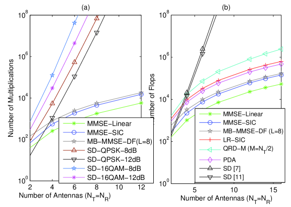
Figure 3: Computational complexity of detection algorithms.

An example of the computational cost of some detection algorithms is shown in Fig. 3, where the number of multiplications and flops per received vector ${\boldsymbol{r}}[i]$ are shown for the proposed MB-MMSE-DF and RLS algorithms, the bounds on the SD reported by [9] and the SD schemes of [7],[12], the complex LR-SIC of [24] with an MMSE filter, the PDA algorithm reported in [17] with $I=5$ iterations, the linear detector and the SIC detector [20]. The complexity evaluated in terms of flops assumes $16$-QAM modulation and ${\rm SNR}=8$ dB and includes the QRD-M detector [25, 26] with $M=8$. The QRD-M algorithm is a breadth-first tree search algorithm, whereas the LSD is a depth-first tree search algorithm that can achieve the optimal performance. Differently from the QRD-M algorithm and the LSD algorithms, the proposed MB-MMSE-DF detector associates branches with different orderings and pairs of linear and feedback filters that only require one matrix inversion. The list of candidates in the MB-MMSE-DF algorithm is different because the candidates are generated by MMSE filtering and feedback cancellation with different orderings, while the list is generated from a tree search in the case of the QRD-M detector and the LSD algorithm. Moreover, the complexity of the MB-MMSE-DF detector only depends on the number of branches regardless of the constellation size and the signal-to-noise ratio (SNR), whereas the complexity of the QRD-M depends on the choice of $M$ and the cost of LSD algorithms is dependent on the constellation size and the SNR. The curves of Fig. 3 indicate that the proposed MB-MMSE-DF and RLS algorithms have a complexity higher than the SIC [20] and significantly lower than the SD algorithms for $N_{R}=N_{T}>4$ and the QRD-M algorithm. The MB-MMSE-DF detector also has a lower complexity than the LR-SIC and the PDA algorithms.

VI-B Diversity Order

The aim of this part is to examine the diversity order achieved by the MB-MMSE-DF detector. In the analysis, it is assumed that the data transmission is over a block fading channel, there is no error propagation due to interference cancellation and that the SNR is sufficiently high [64, 65] (in this case the MMSE and zero-forcing receive filters have a similar behavior). The diversity order [64, 65] is defined by

$$d\triangleq\lim_{\textrm{SNR}\rightarrow\infty}\frac{\log P_{e}(\textrm{SNR})}{\log(\textrm{SNR})},$$ (38)

where $P_{e}$ denotes the probability of error and $\textrm{SNR}=10\log_{10}\frac{N_{T}\sigma_{s}^{2}}{RC~{}\sigma^{2}}$ is the signal-to-noise ratio, $R$ is the rate of the code and $C$ is the number of bits required to map the constellation points. It is known that the diversity order is $d=N_{R}$ for ML receivers and $d=N_{R}-N_{T}+1$ for receivers with SIC [64, 65]. Since for non-ergodic scenarios the error probability is dominated by the outage probability [64, 65], the diversity order can be expressed as

$$d\triangleq\lim_{x\rightarrow\infty}\frac{\log Pr(R_{j,{\rm span}\{1,2,\ldots,j-1,j+1,\ldots,N_{T}\}}\leq x)}{\log(x)},$$ (39)

where $R_{j,{\rm span}\{1,2,\ldots,j-1,j+1,\ldots,N_{T}\}}=R_{j,{\rm span}\{\bar{j}\}}$ is the squared projection height from the $j$th column vector ${\boldsymbol{h}}_{j}$ of ${\boldsymbol{H}}$, i.e., $R_{j,{\rm span}\{\bar{j}\}}=||{\boldsymbol{P}}{\boldsymbol{h}}_{j}||^{2}$, where ${\boldsymbol{P}}={\boldsymbol{I}}-{\boldsymbol{B}}{\boldsymbol{B}}^{H}$ is the projection matrix onto the orthogonal space of ${\rm span}\{\bar{j}\}$, and ${\boldsymbol{B}}$ is composed of any orthogonal basis of this subspace.

Theorem: The diversity order achieved by the MB-MMSE-DF detector is given by

$$\begin{split}d_{\rm MB}&\triangleq\lim_{x\rightarrow 0}\frac{\log Pr(R_{j,l_{j,{\rm opt}},{\rm span}\{\bar{l}_{j,{\rm opt}}\}}\leq x)}{\log(x)}=N_{R}-N_{T}+G,\end{split}$$ (40)

where $1\leq G\leq N_{T}$ is the number of interference free candidates among the $L$ candidates for each stream.

Proof: In order to prove this theorem, it is necessary to make a few assumptions that are common to works that analyze the diversity order of detectors. The approach used to prove the theorem is based on induction and the inclusion of an increasing number of branches that correspond to extra degrees of freedom.

The first assumption is that for each data stream and branch there is an associated diversity order given by $d\triangleq\lim_{x\rightarrow\infty}\frac{\log Pr(R_{j,l,{\rm span}\{\bar{j}\}}\leq x)}{\log(x)}$, as established in [64, 65] for a conventional receiver performing SIC in a MIMO system with $N_{T}$ transmit and $N_{R}$ receive antennas. Another assumption is that the ordering algorithm can exploit the multiple branches to move each data stream to the last position in the sequence of detection to obtain an interference free candidate for detection.

Starting from this point, the result can be extended by induction. By gradually adding branches with different orderings, the number of detection candidates available can be represented by the following sets

$$\begin{split}{\mathcal{S}}_{1}&=\{R_{j,1,{\rm span}\{\bar{j}\}}\},\\ {\mathcal{S}}_{2}&=\{R_{j,1,{\rm span}\{\bar{j}\}},R_{j,2,{\rm span}\{\bar{j}\}}\},\\ \vdots&\\ {\mathcal{S}}_{L}&=\{R_{j,1,{\rm span}\{\bar{j}\}},R_{j,2,{\rm span}\{\bar{j}\}},\ldots,R_{j,L,{\rm span}\{\bar{j}\}}\}.\\ \end{split}$$ (41)

Unlike a conventional receiver with SIC, the proposed MB-MMSE detector has at any given stage $L$ alternatives to select the candidate for detection. In fact, the detection of each stream involves the selection of the best out of $L$ candidate symbols using the rule in (3). The number of degrees of freedom will depend on the quantities $R_{j,l_{j,{\rm opt}},{\rm span}\{\bar{l}_{j,{\rm opt}}\}}$ and wether they correspond to interference free candidates.

By defining $1\leq G\leq N_{T}$ as the number of interference free candidates and assuming that $L>G$ is sufficiently large to provide a sufficiently large number of interference free candidates for the $j$th stream, the diversity order associated with each of the above sets can be described by

$$\begin{split}d_{\rm MB}({\mathcal{S}}_{1})&=\lim_{x\rightarrow 0}\frac{\log Pr(R_{j,l_{j,{\rm opt}},{\rm span}\{\bar{l}_{j,{\rm opt}}\}}\leq x)}{\log(x)}=N_{R}-N_{T}+1,\\ N_{R}-N_{T}+1\leq d_{\rm MB}({\mathcal{S}}_{2})&=\lim_{x\rightarrow 0}\frac{\log Pr(R_{j,l_{j,{\rm opt}},{\rm span}\{\bar{l}_{j,{\rm opt}}\}}\leq x)}{\log(x)}\leq N_{R}-N_{T}+2,\\ \vdots&\\ N_{R}-N_{T}+1\leq d_{\rm MB}({\mathcal{S}}_{L})&=\lim_{x\rightarrow 0}\frac{\log Pr(R_{j,l_{j,{\rm opt}},{\rm span}\{\bar{l}_{j,{\rm opt}}\}}\leq x)}{\log(x)}\leq N_{R}-N_{T}+G.\end{split}$$ (42)

where

$$l_{j,{\rm opt}}=\arg\min_{1\leq l_{j}\leq L}{\rm IMMSE}(\sigma_{s}^{2},{\boldsymbol{w}}_{j,l},{\boldsymbol{f}}_{j,l})$$ (43)

and $R_{j,l_{j,{\rm opt}},{\rm span}\{\bar{l}_{j,{\rm opt}}\}}$ is the squared projection height resulting from the selection of the best out of the available candidates from the set ${\mathcal{S}}_{l}$ for the $j$th stream. If interference free candidates are gradually included in the sets and are selected by the above procedure, then the MB-MMSE-DF detector can obtain $G$ interference free candidates resulting from $N_{T}-1$ cancellations for any branch. Hence, the diversity order for each stream of the MB-MMSE-DF detector is given by

$$\begin{split}d_{\rm MB}&\triangleq\lim_{x\rightarrow 0}\frac{\log Pr(R_{j,l_{j,{\rm opt}},{\rm span}\{\bar{l}_{j,{\rm opt}}\}}\leq x)}{\log(x)}=N_{R}-N_{T}+G.\end{split}$$ (44)

This suggests that the key advantage of the MB-MMSE-DF detector is its ability to generate $L$ candidates for each stream and select $G$ interference free candidates. In practice, $G$ will depend on the number of branches used, the ordering algorithm and the accuracy of the interference cancellation.

VII Simulations

In this section, the bit error ratio (BER) performance of the MB-MMSE-DF and other relevant MIMO detection schemes is evaluated. The sphere decoder (SD) [12], the linear [13], the SIC [15], the QRD-M [25, 26] with $M=8$, the PDA [27, 59] with $I=5$ iterations, MMSE estimators and the proposed MB-MMSE-DF techniques without and with error propagation mitigation techniques are considered in the simulations. The lattice-reduction aided versions of the linear and the SIC detectors [24], which are denoted LR-MMSE-Linear and LR-MMSE-SIC, respectively, are also included in the study. The channel coefficients are either static and obtained from complex Gaussian random variables with zero mean and unit variance, or time-varying with the coefficients given by the Jakes model [66]. The modulation employed is either QPSK or $16$-QAM. Both uncoded and coded systems are considered. For the coded systems and iterative detection and decoding, a non-recursive convolutional code with rate $R=1/2$, constraint length $3$, generator polynomial $g=[7~{}5]_{\rm oct}$ and $5$ decoding iterations is adopted. The numerical results are averaged over $10^{6}$ runs, packets with $Q=500$ symbols for uncoded systems and $Q=1000$ coded symbols are employed and the signal-to-noise ratio (SNR) in dB is defined as $\textrm{SNR}=10\log_{10}\frac{N_{T}\sigma_{s}^{2}}{RC~{}\sigma^{2}}$, where $\sigma_{s}^{2}$ is the variance of the symbols, $\sigma^{2}$ is the noise variance, $R<1$ is the rate of the channel code and $C$ is the number of bits used to represent the constellation.

In the first example, the ordering algorithms described in Section IV are assessed with the MB-MMSE-DF detector using $L=1,2,{\rm and}~{}4$ branches. A MIMO system with $N_{T}=N_{R}=4$ antennas is considered with perfect channel estimation. The BER performance of the MB-MMSE-DF detector is evaluated with the optimal and the suboptimal ordering algorithms and the curves are shown in Fig. 4. The results show that the suboptimal ordering algorithm is able to approach the performance of the optimal ordering algorithm that performs an exhaustive search. In particular, the BER performance gap between the optimal and suboptimal ordering algorithms is small and this has also been observed for larger systems and a different number of branches $L$. For this reason, the suboptimal ordering algorithm has been adopted in the next examples.

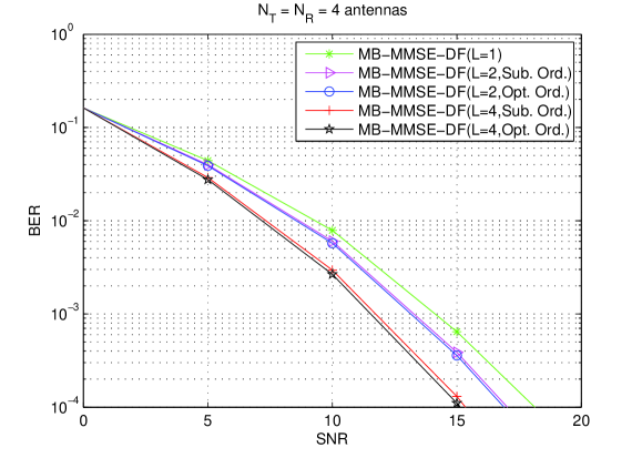
Figure 4: BER performance of the optimal and the proposed suboptimal ordering algorithms .

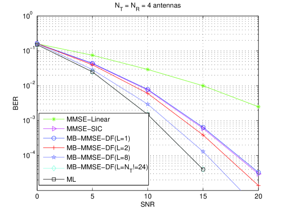
Figure 5: BER performance of the detectors with perfect channel estimation for multiple branches $L$ and QPSK.

The uncoded BER performance of the proposed MB-MMSE-DF detector is then considered in an example to evaluate the number of branches that should be used in the suboptimal ordering algorithm. It is also important to account for the impact of additional branches on the performance with perfect channel estimation for a MIMO system with $N_{T}=N_{R}=4$ antennas. The proposed suboptimal ordering algorithm is compared against the optimal ordering approach described in Section IV that evaluates $N_{T}!=24$ possible branches. The MB-MMSE-DF detector has been designed with $L=2~{}{\rm and}~{}4$ parallel branches and its BER performance against the SNR has been compared with those of the existing schemes, as depicted in Fig. 5. In fact, the MB-MMSE-DF detector is able to gradually approach the BER performance of the ML detector as the number of branches L is increased. Starting with L=1, the MB-MMSE-DF detector has a BER performance comparable with that of a standard MMSE-SIC detector. By increasing L the BER performance of MB-MMSE-DF gradually improves and gets within 1.5 dB of SNR for the same BER performance as the ML detector when L=8. Finally, MB-MMSE-DF obtains a performance that is comparable (the curves coincide) when L=24.

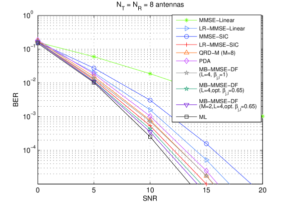
Figure 6: BER performance with adaptive estimation and QPSK modulation.

In the next experiments depicted in Figs. 6 and 7, the uncoded BER performance of the proposed MB-MMSE-DF detector is evaluated with $L=4$, $N_{T}=N_{R}=8$ antennas, QPSK and $16$-QAM modulation, a block fading channel and adaptive estimation using the proposed RLS-type algorithm with $\hat{\boldsymbol{R}}^{-1}[0]=10^{-2}{\boldsymbol{I}}$ and $\lambda=0.998$. In the transmission, we assume packets with $500$ symbols and employ a training sequence with $N_{Tr}=50$ symbols to compute the channel and the receive filter coefficients. We include in the comparison the linear and SIC detectors with RLS algorithms, the LR-MMSE-Linear and LR-MMSE-SIC detection schemes [24] using MMSE filters, the QRD-M technique of [25, 26], the PDA algorithm of [27] and the SD of [12] to compute the ML solution, which employ the RLS algorithm to estimate the channels.

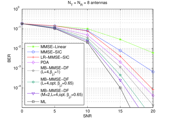
Figure 7: BER performance with adaptive estimation and $16-$QAM.

The results depicted in Figs. 6 and 7 for QPSK and $16$-QAM, respectively, show that the proposed MB-MMSE-DF detector achieves a performance which is close to the ML solutions implemented with the SD and outperforms the linear, the SIC, the LR-MMSE-Linear, LR-MMSE-SIC, the QRD-M and the PDA detectors by a significant margin. In particular, the proposed MB-MMSE-DF detector with $L=4$ without error propagation mitigation ($\beta_{j,l}=\gamma_{j,l}=1$) has a comparable performance to the PDA and the LR-MMSE-SIC detectors, whereas the MB-MMSE-DF scheme with an optimized value of $\beta_{j,l}=0.65$ outperforms the PDA and the LR-MMSE-SIC schemes. The MB-MMSE-DF scheme with $M=2$ stages and $L=4$ significantly outperforms the QRD-M, the PDA and the LR-MMSE-SIC algorithms and achieves a performance within $1$ dB from the ML solution, while requiring a cost comparable to the SIC with the RLS algorithm.

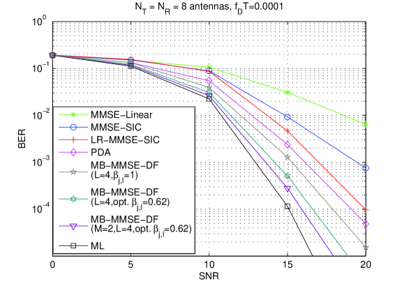
Figure 8: BER performance with adaptive estimation and $16-$QAM in time-varying channels with $f_{D}T=10^{-4}$.

In the next two examples, the uncoded and coded BER performances of the detectors are assessed for systems with $16$-QAM modulation and time-varying channels. The channel coefficients in these examples change every received vector according to the Jakes model [66] and the results are shown in terms of the normalized Doppler frequency $f_{D}T$ (cycles/symbol), where $f_{D}$ is the maximum Doppler shift and $T$ is the symbol interval. For the data transmission, packets with $Q=500$ symbols are used for the uncoded system, with $Q=1000$ coded symbols for the convolutionally coded system with 5 decoding iterations, and a training sequence with $N_{Tr}=50$ symbols is employed to compute the channel and receive filter coefficients. After the training sequence, the receivers are switched to decision-directed mode and the parameters are tracked with RLS-type algorithms.

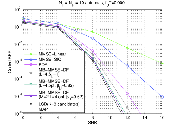
Figure 9: Coded BER performance with adaptive estimation and $16-$QAM in time-varying channels with $f_{D}T=10^{-4}$ and 5 decoding iterations.

The uncoded BER results illustrated in Fig. 8 show similar results to that of Fig. 7 but with a slight performance degradation due to the time-varying nature of the channel. The coded BER performance illustrated in Fig. 9 indicates that the proposed iterative MB-MMSE-DF detector with an optimized value of $\beta_{j,l}=0.62$, $L=4$ and $M=2$ has a performance that is very close to the optimal MAP detector and is comparable to the list SD (LSD) with $K=8$ candidates, which corresponds to the SD of [12] with LLR processing. The proposed iterative MB-MMSE-DF detector has a gain of up to $2$ dB over the PDA detector and of up to $5$ dB over the conventional SIC with iterative processing for the same coded BER, while the computational cost of MB-MMSE-DF is significantly lower than the PDA technique and slightly higher than the SIC algorithm.

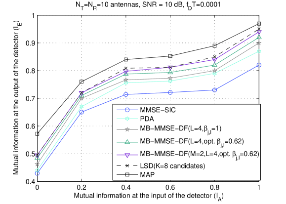
Figure 10: EXIT chart for the analyzed detectors with $16-$QAM.

In Fig. 10, the soft input and output behavior of the detection algorithms is described through the use of the extrinsic information transfer (EXIT) chart [67] analysis. In this plot, $16$-QAM modulation with a $10\times 10$ MIMO system are considered. The quantities $I_{A}$ and $I_{E}$ represent the mutual information at the input and at the output of the detectors analyzed. The proposed MB-MMSE-DF detector is able to achieve a higher capacity compared to the other suboptimal algorithms considered and to follow closely the trajectory of the LSD and MAP algorithms. Specifically, with the increased number of branches, more tentative decisions or candidates are included in the search space for the solution and this allows the proposed MB-MMSE-DF detector to approach the performance of the MAP algorithm.

VIII Concluding Remarks

This work has proposed and investigated MB-MMSE-DF detection algorithms for large MIMO systems using spatial multiplexing. Constrained MMSE filters designed with constraints on the shape and magnitude of the feedback filters have been presented for the MB-MMSE-DF detector and it has been shown that the proposed design does not require a significant additional complexity over the conventional MMSE-DF detector. Optimal and sub-optimal ordering algorithms have also been presented for the MB-MMSE-DF detector. An adaptive version of the MB-MMSE-DF detector has been developed with an RLS-type algorithm for estimating the parameters of the filters when the channel is time-varying. A soft-output version of the MB-MMSE DF detector has also been proposed as a component of an iterative detection and decoding receiver structure. The results have shown that the proposed MB-MMSE-DF detector achieves a performance superior to some existing suboptimal detectors and close to the ML detector, while requiring significantly lower complexity.

Appendix A Derivation of MMSE Receive Filters

In order to derive the MMSE receive filters resulting from the constrained optimization problem presented in (6), the method of Lagrange multipliers is used which results in the following unconstrained cost function

$$\begin{split}{\mathcal{L}}({\boldsymbol{w}}_{j,l},{\boldsymbol{f}}_{j,l},{\boldsymbol{\alpha}}_{j,l},\mu_{j,l})&=E[|s_{j}[i]-{\boldsymbol{w}}_{j,l}^{H}{\boldsymbol{r}}[i]+{\boldsymbol{f}}_{j,l}^{H}\hat{\boldsymbol{s}}_{l}[i]|^{2}]+2\Re[({\boldsymbol{S}}_{j,l}{\boldsymbol{f}}_{j,l})^{H}{\boldsymbol{\alpha}}_{j,l}]\\ &\quad+2\Re[({\boldsymbol{f}}_{j,l}^{H}{\boldsymbol{f}}_{j,l}-\gamma_{j,l}{\boldsymbol{f}}_{j,l}^{H,~{}c}{\boldsymbol{f}}_{j,l}^{c})^{H}\mu_{j,l}],~{}~{}j=1,\ldots,N_{T},~{}l=1,\ldots,L,\end{split}$$ (45)

where ${\boldsymbol{\alpha}}_{j,l}$ is an $N_{T}\times 1$ vector of Lagrange multipliers and $\mu_{j,l}$ is a scalar Lagrange multiplier.

By computing the gradient terms of (45) with respect to ${\boldsymbol{w}}_{j,l}^{*}$ and equating them to zero, we have

$$\nabla{\mathcal{L}}({\boldsymbol{w}}_{j,l},{\boldsymbol{f}}_{j,l},{\boldsymbol{\alpha}}_{j,l},\mu_{j,l})_{{\boldsymbol{w}}_{j,l}^{*}}=E[-{\boldsymbol{r}}[i](s_{j}[i]-{\boldsymbol{w}}_{j,l}^{H}{\boldsymbol{r}}[i]+{\boldsymbol{f}}_{j,l}^{H}\hat{\boldsymbol{s}}_{l}[i])^{*}]={\boldsymbol{0}}$$ (46)

By further manipulating the terms in the above equation, we arrive at the expression obtained in (7)

$${\boldsymbol{w}}_{j,l}^{\rm MMSE}={\boldsymbol{R}}^{-1}({\boldsymbol{p}}_{j}+{\boldsymbol{Q}}{\boldsymbol{f}}_{j,l}),$$ (47)

where ${\boldsymbol{R}}=E[{\boldsymbol{r}}[i]{\boldsymbol{r}}^{H}[i]]$ is the $N_{R}\times N_{R}$ covariance matrix of the received data, ${\boldsymbol{p}}_{j}=E[{\boldsymbol{r}}[i]s_{j}^{*}[i]]$ is the $N_{R}\times 1$ cross-correlation vector and ${\boldsymbol{Q}}=E[{\boldsymbol{r}}[i]\hat{\boldsymbol{s}}_{l}^{H}[i]]$ is a $N_{R}\times N_{T}$ cross-correlation matrix.

By calculating the gradient terms of (45) with respect to ${\boldsymbol{f}}_{j,l}^{*}$ and equating them to zero, we have

$$\vspace{-0.25em}\nabla{\mathcal{L}}({\boldsymbol{w}}_{j,l},{\boldsymbol{f}}_{j,l},{\boldsymbol{\alpha}}_{j,l},\mu_{j,l})_{{\boldsymbol{f}}_{j,l}^{*}}=E[\hat{\boldsymbol{s}}_{l}[i](s_{j}[i]-{\boldsymbol{w}}_{j,l}^{H}{\boldsymbol{r}}[i]+{\boldsymbol{f}}_{j,l}^{H}\hat{\boldsymbol{s}}_{l}[i])^{*}]+2{\boldsymbol{S}}_{j,l}{\boldsymbol{\alpha}}_{j,l}+2{\boldsymbol{f}}_{j,l}\mu_{j,l}={\boldsymbol{0}}$$ (48)

Using the above equation and with further manipulations, we obtain

$$\vspace{-0.25em}{\boldsymbol{f}}_{j,l}^{\rm MMSE}=\frac{\beta_{j,l}}{\sigma_{s}^{2}}({\boldsymbol{Q}}^{H}{\boldsymbol{w}}_{j,l}-{\boldsymbol{t}}_{j}-2{\boldsymbol{S}}_{j,l}^{H}{\boldsymbol{\alpha}}_{j,l}).$$ (49)

where the term $\beta_{j,l}=(1-2\mu_{j,l})^{-1}$ with the Lagrange multiplier $\mu_{j,l}$ is responsible for the mitigation of the error propagation and is a parameter to be adjusted, and $E[\hat{\boldsymbol{s}}[i]{\boldsymbol{s}}^{H}[i]]=\sigma_{s}^{2}{\boldsymbol{I}}$ since it is assumed that $\hat{\boldsymbol{s}}[i]$ has independent and identically distributed entries. The above expression describes the relationship between the feedback filters ${\boldsymbol{f}}_{j,l}^{\rm opt}$, the feedforward filter ${\boldsymbol{w}}_{j,l}^{\rm opt}$ and the quantities ${\boldsymbol{Q}}$, ${\boldsymbol{t}}_{j}=E[\hat{\boldsymbol{s}}_{l}[i]s_{j}[i]]$, and the Lagrange multipliers $\mu_{j,l}$ and ${\boldsymbol{\alpha}}_{j,l}$.

The expression for the Lagrange multiplier ${\boldsymbol{\alpha}}_{j,l}$ can be obtained by computing the gradient terms of (45) with respect to ${\boldsymbol{\alpha}}_{j,l}$ and equating them to zero, which results in

$$\nabla{\mathcal{L}}({\boldsymbol{w}}_{j,l},{\boldsymbol{f}}_{j,l},{\boldsymbol{\alpha}}_{j,l},\mu_{j,l})_{{\boldsymbol{\alpha}}_{j,l}}={\boldsymbol{S}}_{j,l}{\boldsymbol{f}}_{j,l}={\boldsymbol{0}}$$ (50)

By substituting (49) into the above expression and solving for ${\boldsymbol{\alpha}}_{j,l}$, we have

$$\vspace{-0.25em}{\boldsymbol{\alpha}}_{j,l}=({\boldsymbol{S}}_{j,l}{\boldsymbol{S}}_{j,l}^{H})^{-1}\big{(}{\boldsymbol{S}}_{j,l}^{H}{\boldsymbol{Q}}^{H}{\boldsymbol{w}}_{j,l}-{\boldsymbol{S}}_{j,l}{\boldsymbol{t}}_{j}\big{)}/2,$$ (51)

It turns out that there is no closed form solution for the term $\beta_{j,l}$, which is a function of the Lagrange multiplier $\mu_{j,l}$. This happens because its evaluation leads to a quadratic function of the feedback filter ${\boldsymbol{f}}_{j,l}$ that is quite involved. For this reason, we employ an approach that computes $\beta_{j,l}$ numerically. By inserting the expression for ${\boldsymbol{\alpha}}_{j,l}$ into (49), we arrive at

$${\boldsymbol{f}}_{j,l}^{\rm MMSE}=\frac{\beta_{j,l}}{\sigma_{s}^{2}}\Big{(}{\boldsymbol{Q}}^{H}{\boldsymbol{w}}_{j,l}-{\boldsymbol{t}}_{j}-{\boldsymbol{S}}_{j,l}^{H}({\boldsymbol{S}}_{j,l}{\boldsymbol{S}}_{j,l}^{H})^{-1}\big{(}{\boldsymbol{S}}_{j,l}^{H}{\boldsymbol{Q}}^{H}{\boldsymbol{w}}_{j,l}-{\boldsymbol{S}}_{j,l}{\boldsymbol{t}}_{j}\big{)}\Big{)},$$ (52)

where ${\boldsymbol{f}}_{j,l}^{\rm MMSE}$ is a function of the Lagrange multiplier $\mu_{j,l}$. By defining ${\boldsymbol{\Pi}}_{j,l}={\boldsymbol{I}}-{\boldsymbol{S}}_{j,l}^{H}({\boldsymbol{S}}_{j,l}^{H}{\boldsymbol{S}}_{j,l})^{-1}{\boldsymbol{S}}_{j,l}$ as a projection matrix that ensures the shape constraint ${\boldsymbol{S}}_{j,l}$, the above expression can be written as (8) in the compact form

$$\begin{split}{\boldsymbol{f}}_{j,l}^{\rm MMSE}&=\frac{\beta_{j,l}}{\sigma_{s}^{2}}{\boldsymbol{\Pi}}_{j,l}({\boldsymbol{Q}}^{H}{\boldsymbol{w}}_{j,l}-{\boldsymbol{t}}_{j}),\end{split}$$ (53)

Now if we substitute the above expression into (47) and further manipulate the expressions, we obtain

$$\vspace{-0.25em}{\boldsymbol{w}}_{j,l}^{\rm MMSE}=({\boldsymbol{R}}-\beta_{j,l}{\boldsymbol{Q}}{\boldsymbol{\Pi}}_{j,l}{\boldsymbol{Q}}^{H})^{-1}\big{(}{\boldsymbol{p}}_{j}-\beta_{j,l}{\boldsymbol{Q}}{\boldsymbol{\Pi}}_{j,l}{\boldsymbol{t}}_{j}\big{)}.$$ (54)

Substituting the above expression into (53), we obtain

$$\begin{split}{\boldsymbol{f}}_{j,l}^{\rm MMSE}&=\frac{\beta_{j,l}}{\sigma_{s}^{2}}{\boldsymbol{\Pi}}_{j,l}\Big{[}{\boldsymbol{Q}}^{H}({\boldsymbol{R}}-\beta_{j,l}{\boldsymbol{Q}}{\boldsymbol{\Pi}}_{j,l}{\boldsymbol{Q}}^{H})^{-1}\big{(}{\boldsymbol{p}}_{j}-\beta_{j,l}{\boldsymbol{Q}}{\boldsymbol{\Pi}}_{j,l}{\boldsymbol{t}}_{j}\big{)}-{\boldsymbol{t}}_{j}\Big{]},\end{split}$$ (55)

where the above expressions for the receive filters ${\boldsymbol{w}}_{j,l}$ and ${\boldsymbol{f}}_{j,l}$ only depend on the statistical quantities ${\boldsymbol{R}}$, ${\boldsymbol{Q}}$, ${\boldsymbol{t}}_{j}$ and ${\boldsymbol{p}}_{j}$ and the parameters $\beta_{j,l}$ and ${\boldsymbol{\Pi}}_{j,l}$. Nevertheless, these expressions have an inconvenient form for practical use as they require multiple matrix inversions for the computation of the receiver filters for each data stream $j$ and branch $l$. To circumvent this drawback, the use of an alternating strategy with (47) and (52) is employed as it allows a designer to compute only one matrix inversion (${\boldsymbol{R}}^{-1}$) and all the receive filters with a reduced number of extra multiplications and additions.

The expressions obtained so far can be simplified by evaluating some of the key statistical quantities such as ${\boldsymbol{R}}$, ${\boldsymbol{Q}}$, ${\boldsymbol{t}}_{j}$ and ${\boldsymbol{p}}_{j}$ and replacing them in the formulas for the receive filters. Using the fact that the quantity ${\boldsymbol{t}}_{j}={\boldsymbol{0}}$ for interference cancellation, ${\boldsymbol{v}}_{j,l}={\boldsymbol{0}}$, and assuming perfect feedback (${\boldsymbol{s}}=\hat{\boldsymbol{s}}$) we have

$$\begin{split}{\boldsymbol{R}}&={\sigma_{s}}^{2}{\boldsymbol{H}}{\boldsymbol{H}}^{H}+{\sigma_{n}^{2}}{\boldsymbol{I}},{\boldsymbol{Q}}={\sigma_{s}}^{2}{\boldsymbol{H}},{\boldsymbol{p}}_{j}={\sigma_{s}}^{2}{\boldsymbol{H}}{\boldsymbol{\delta}}_{j},\end{split}$$ (56)

where ${\boldsymbol{\delta}}_{j}=[\underbrace{0\ldots 0}_{j-1}~{}1~{}\underbrace{0\ldots 0}_{N_{T}-j-2}]^{T}$ is a $N_{T}\times 1$ vector with a one in the $j$th element and zeros elsewhere. Substituting ${\boldsymbol{t}}_{j}={\boldsymbol{0}}$ and (56) into (47) and (52) we arrive at (12) and (13), respectively.

Appendix B MMSE Expressions and Connections with Conventional DF Receivers

The MMSE associated with the filters ${\boldsymbol{w}}_{j,l}$ and ${\boldsymbol{f}}_{j,l}$ and the statistics of the data symbols $s_{j}[i]$ is given by

$$\begin{split}\underbrace{{\rm MMSE}(s_{j}[i],{\boldsymbol{w}}_{j,l}^{\rm MMSE},{\boldsymbol{f}}_{j,l}^{\rm MMSE})}_{{\rm MMSE}_{j}}&=E[|s_{j}[i]-{\boldsymbol{w}}_{j,l}^{H}{\boldsymbol{r}}[i]+{\boldsymbol{f}}_{j,l}^{H}{\boldsymbol{s}}_{l}[i]|^{2}]\\ &=\underbrace{E[|s_{j}[i]|^{2}]}_{\sigma_{s}^{2}}-{\boldsymbol{w}}_{j,l}^{H}\underbrace{E[{\boldsymbol{r}}[i]s_{j}^{*}[i]]}_{{\boldsymbol{p}}_{j}}-\underbrace{E[{\boldsymbol{r}}^{H}[i]s_{j}[i]]}_{{\boldsymbol{p}}_{j}^{H}}{\boldsymbol{w}}_{j,l}+{\boldsymbol{w}}_{j,l}^{H}\underbrace{E[{\boldsymbol{r}}[i]{\boldsymbol{r}}^{H}[i]]}_{\boldsymbol{R}}{\boldsymbol{w}}_{j,l}\\ &\quad-{\boldsymbol{w}}_{j,l}^{H}\underbrace{E[{\boldsymbol{r}}[i]{\boldsymbol{s}}_{l}^{H}[i]]}_{{\boldsymbol{Q}}}{\boldsymbol{f}}_{j,l}-{\boldsymbol{f}}_{j,l}^{H}{\boldsymbol{Q}}^{H}{\boldsymbol{w}}_{j,l}+{\boldsymbol{f}}_{j,l}^{H}\underbrace{E[{\boldsymbol{s}}_{l}s_{j}^{*}[i]]}_{{\boldsymbol{t}}_{j}}+{\boldsymbol{t}}_{j}^{H}{\boldsymbol{f}}_{j,l}+{\boldsymbol{f}}_{j,l}^{H}\underbrace{E[{\boldsymbol{s}}_{l}{\boldsymbol{s}}_{l}^{H}]}_{\bf I}{\boldsymbol{f}}_{j,l}\\ &=\sigma_{s}^{2}-{\boldsymbol{w}}_{j,l}^{H}{\boldsymbol{p}}_{j}-{\boldsymbol{p}}_{j}^{H}{\boldsymbol{w}}_{j,l}+{\boldsymbol{w}}_{j,l}^{H}{\boldsymbol{R}}{\boldsymbol{w}}_{j,l}-{\boldsymbol{w}}_{j,l}^{H}{\boldsymbol{Q}}{\boldsymbol{f}}_{j,l}-{\boldsymbol{f}}_{j,l}^{H}{\boldsymbol{Q}}^{H}{\boldsymbol{w}}_{j,l}+{\boldsymbol{f}}_{j,l}^{H}{\boldsymbol{t}}_{j}+{\boldsymbol{t}}_{j}^{H}{\boldsymbol{f}}_{j,l}+{\boldsymbol{f}}_{j,l}^{H}{\boldsymbol{f}}_{j,l}\\ &=\sigma_{s}^{2}-{\boldsymbol{w}}_{j,l}^{H}{\boldsymbol{p}}_{j}-{\boldsymbol{p}}_{j}^{H}{\boldsymbol{w}}_{j,l}+\underbrace{({\boldsymbol{f}}_{j,l}^{H}{\boldsymbol{Q}}^{H}+{\boldsymbol{p}}_{j}^{H})}_{{\boldsymbol{w}}_{j,l}}{\boldsymbol{R}}^{-1}{\boldsymbol{w}}_{j,l}\\ &\quad-{\boldsymbol{w}}_{j,l}^{H}{\boldsymbol{Q}}{\boldsymbol{f}}_{j,l}-{\boldsymbol{f}}_{j,l}^{H}{\boldsymbol{Q}}^{H}{\boldsymbol{w}}_{j,l}+{\boldsymbol{f}}_{j,l}^{H}{\boldsymbol{t}}_{j}+{\boldsymbol{t}}_{j}^{H}{\boldsymbol{f}}_{j,l}+{\boldsymbol{f}}_{j,l}^{H}{\boldsymbol{f}}_{j,l}\\ &=\sigma_{s}^{2}-{\boldsymbol{w}}_{j,l}^{H}{\boldsymbol{R}}{\boldsymbol{w}}_{j,l}+{\boldsymbol{t}}_{j}^{H}{\boldsymbol{f}}_{j,l}+{\boldsymbol{f}}_{j,l}^{H}{\boldsymbol{t}}_{j}+{\boldsymbol{f}}_{j,l}^{H}{\boldsymbol{f}}_{j,l}.\end{split}$$ (57)

By substituting ${\boldsymbol{t}}_{j}={\boldsymbol{0}}$, the quantities in (56) and the expressions in (54) and (55), the MMSE becomes

$$\vspace{-0.25em}\begin{split}{\rm MMSE}_{j}&=\sigma_{s}^{2}-{\boldsymbol{w}}_{j,l}^{H,~{}{\rm MMSE}}{\boldsymbol{R}}{\boldsymbol{w}}_{j,l}^{\rm MMSE}+{\boldsymbol{f}}_{j,l}^{H,~{}{\rm MMSE}}{\boldsymbol{f}}_{j,l}^{\rm opt}\\ &=\sigma_{s}^{2}-{\boldsymbol{p}}_{j}^{H}({\boldsymbol{R}}-\beta_{j,l}{\boldsymbol{Q}}{\boldsymbol{\Pi}}_{j,l}{\boldsymbol{Q}}^{H})^{-1}{\boldsymbol{R}}({\boldsymbol{R}}-\beta_{j,l}{\boldsymbol{Q}}{\boldsymbol{\Pi}}_{j,l}{\boldsymbol{Q}}^{H})^{-1}{\boldsymbol{p}}_{j}\\ &\quad+\beta_{j,l}^{2}{\boldsymbol{p}}_{j}^{H}({\boldsymbol{R}}-\beta_{j,l}{\boldsymbol{Q}}{\boldsymbol{\Pi}}_{j,l}{\boldsymbol{Q}}^{H})^{-1}{\boldsymbol{Q}}{\boldsymbol{\Pi}}_{j,l}^{H}{\boldsymbol{\Pi}}_{j,l}{\boldsymbol{Q}}^{H}({\boldsymbol{R}}-\beta_{j,l}{\boldsymbol{Q}}{\boldsymbol{\Pi}}_{j,l}{\boldsymbol{Q}}^{H})^{-1}{\boldsymbol{p}}_{j}.\end{split}$$ (58)

For a given ordering and branch $l$, the sum of the MMSE in (58) over the $N_{T}$ data streams is equivalent to the MMSE achieved by a conventional MMSE-DF receiver (C-MMSE-DF) and is given by

$$\vspace{-0.25em}{\rm SMMSE}=\sum_{j=1}^{N_{T}}MMSE_{j}$$ (59)

An instantaneous MMSE metric for the selection of the best branch for each received vector can be obtained by removing the expected value from the expression in (57) and considering each received data vector ${\boldsymbol{r}}[i]$, which results in

$$\begin{split}{\rm IMMSE}(s_{j}[i],{\boldsymbol{w}}_{j,l},{\boldsymbol{f}}_{j,l},{\boldsymbol{r}}[i])&=|s_{j}[i]-{\boldsymbol{w}}_{j,l}^{H}{\boldsymbol{r}}[i]+{\boldsymbol{f}}_{j,l}^{H}{\boldsymbol{s}}_{l}[i]|^{2}\\ &={|s_{j}[i]|^{2}}-{\boldsymbol{w}}_{j,l}^{H}\underbrace{{\boldsymbol{r}}[i]s_{j}^{*}[i]}_{\hat{\boldsymbol{p}}_{j}}-\underbrace{{\boldsymbol{r}}^{H}[i]s_{j}[i]}_{\hat{\boldsymbol{p}}_{j}^{H}}{\boldsymbol{w}}_{j,l}+{\boldsymbol{w}}_{j,l}^{H}\underbrace{{\boldsymbol{r}}[i]{\boldsymbol{r}}^{H}[i]}_{\hat{\boldsymbol{R}}}{\boldsymbol{w}}_{j,l}\\ &\quad-{\boldsymbol{w}}_{j,l}^{H}\underbrace{{\boldsymbol{r}}[i]{\boldsymbol{s}}_{l}^{H}[i]}_{\hat{\boldsymbol{Q}}}{\boldsymbol{f}}_{j,l}-{\boldsymbol{f}}_{j,l}^{H}\hat{\boldsymbol{Q}}^{H}{\boldsymbol{w}}_{j,l}+{\boldsymbol{f}}_{j,l}^{H}\underbrace{{\boldsymbol{s}}_{l}s_{j}^{*}[i]}_{\hat{\boldsymbol{t}}_{j}}+{\boldsymbol{t}}_{j}^{H}{\boldsymbol{f}}_{j,l}+{\boldsymbol{f}}_{j,l}^{H}{\boldsymbol{s}}_{l}{\boldsymbol{s}}_{l}^{H}{\boldsymbol{f}}_{j,l}.\end{split}$$ (60)

The expression above suggests that in order to obtain an instantaneous MMSE metric, the MB-MMSE-DF detector needs to compute all the terms. However, it is possible to obtain an effective and yet more efficient expression by inspecting the terms in the first line of (58) and retaining the corresponding instantaneous values, which results in

$${\rm IMMSE}(s_{j}[i],{\boldsymbol{w}}_{j,l},{\boldsymbol{f}}_{j,l},{\boldsymbol{r}}[i])\approx|s_{j}[i]|^{2}-{\boldsymbol{w}}_{j,l}^{H,~{}{\rm MMSE}}\hat{\boldsymbol{R}}{\boldsymbol{w}}_{j,l}^{\rm MMSE}+{\boldsymbol{f}}_{j,l}^{H,~{}{\rm MMSE}}{\boldsymbol{s}}_{l}{\boldsymbol{s}}_{l}^{H}{\boldsymbol{f}}_{j,l}^{\rm MMSE}.$$ (61)

The expression in (61) has been tested and compared with (60), and the results indicate an equivalent performance of the two expressions. Due to the smaller number of terms, the expression in (61) has been adopted for the operation of the MB-MMSE-DF detector.

References

- [1] G. J. Foschini and M. J. Gans, “On limits of wireless communications in a fading environment when using multiple antennas”, Wireless Pers. Commun., vol. 6, pp. 311335, Mar. 1998.
- [2] I. E. Telatar, “Capacity of Multi-Antenna Gaussian Channels”, Eur. Trans. Telecommun., vol. 10, no. 6, pp. 585-595, 1999.
- [3] S. Alamouti, “A simple transmit diversity technique for wireless communications”, IEEE Journal on Selected Areas in Communications, vol. 16, no. 8, pp. 1451-1458, Oct. 1998.
- [4] V. Tarokh, H. Jafarkhani, and A. R. Calderbank, “Space-time block codes from orthogonal designs,” IEEE Trans. Inf. Theory, vol. 45, pp. 1456-1467, July 1999.
- [5] S. Verdu, Multiuser Detection, Cambridge, 1998.
- [6] E. Viterbo and J. Boutros, “A universal lattice code decoder for fading channels”, IEEE Trans. on Inf. Theory, vol. 45, no. 5, pp.1639–1642, July 1999.
- [7] M. O. Damen, H. E. Gamal, and G. Caire, “On maximum likelihood detection and the search for the closest lattice point,” IEEE Trans. Inform. Theory, vol. 49, pp. 2389–2402, Oct. 2003.
- [8] H. Vikalo, B. Hassibi, and T. Kailath, Iterative decoding for MIMO channels via modified sphere decoding,” IEEE Trans. Wireless Commun., vol. 3, pp. 2299-2311, Nov. 2004.
- [9] B. Hassibi and H. Vikalo, “On the sphere decoding algorithm: Part I, the expected complexity”, IEEE Trans. on Signal Processing, vol 53, no. 8, pp. 2806-2818, Aug 2005.
- [10] Z. Guo and P. Nilsson, “Algorithm and Implementation of the K-Best Sphere Decoding for MIMO Detection,” IEEE Journal on Selected Areas in Communications, vol. 24, no. 3, pp. 491–503, March 2006.
- [11] C. Studer, A. Burg, and H. Bolcskei, Soft-output sphere decoding: algorithms and VLSI implementation,” IEEE J. Sel. Areas Commun., vol. 26, pp. 290-300, Feb. 2008.
- [12] B. Shim and I. Kang, “On further reduction of complexity in tree pruning based sphere search,” IEEE Trans. Commun., vol. 58, no. 2, pp. 417–422, Feb. 2010.
- [13] A. Duel-Hallen, “Equalizers for Multiple Input Multiple Output Channels and PAM Systems with Cyclostationary Input Sequences,” IEEE J. Select. Areas Commun., vol. 10, pp. 630-639, April, 1992.
- [14] R. C. de Lamare, R. Sampaio-Neto, ”Blind Adaptive MIMO Receivers for Space-Time Block-Coded DS-CDMA Systems in Multipath Channels Using the Constant Modulus Criterion”, IEEE Trans. on Commun., vol. 58, no. 1, Jan. 2010
- [15] G. D. Golden, C. J. Foschini, R. A. Valenzuela and P. W. Wolniansky, “Detection algorithm and initial laboratory results using V-BLAST space-time communication architecture”, Electronics Letters, vol. 35, No.1, January 1999.
- [16] J. Benesty, Y. Huang, and J. Chen, “A fast recursive algorithm for optimum sequential signal detection in a BLAST system,” IEEE Trans. Signal Processing, vol. 51, pp. 1722–1730, July 2003.
- [17] Y. Shang and X.-G. Xia, “An improved fast recursive algorithm for V-BLAST with optimal ordered detections,” in Proc. IEEE ICC 2008, Beijing, China, May 2008, pp. 756–760.
- [18] N. Al-Dhahir and A. H. Sayed, ”The finite-length multi-input multi-output MMSE-DFE,” IEEE Trans. on Signal Processing, vol. 48, no. 10, pp. 2921-2936, Oct., 2000.
- [19] J. H. Choi, H. Y. Yu, Y. H. Lee, ”Adaptive MIMO decision feedback equalization for receivers with time-varying channels”, IEEE Trans. Signal Proc., 2005, 53, no. 11, pp. 4295-4303.
- [20] A. Rontogiannis, V. Kekatos, and K. Berberidis,” A Square-Root Adaptive V-BLAST Algorithm for Fast Time-Varying MIMO Channels,” IEEE Signal Processing Letters, Vol. 13, No. 5, pp. 265-268, May 2006.
- [21] R. Fa, R. C. de Lamare, “Multi-Branch Successive Interference Cancellation for MIMO Spatial Multiplexing Systems”, IET Communications, vol. 5, no. 4, pp. 484 - 494, March 2011.
- [22] P. Li, R. C. de Lamare and R. Fa, “Multiple Feedback Successive Interference Cancellation Detection for Multiuser MIMO Systems,” IEEE Transactions on Wireless Communications, vol. 10, no. 8, pp. 2434 - 2439, August 2011.
- [23] C. Windpassinger, L. Lampe, R.F.H. Fischer, T.A Hehn, “A performance study of MIMO detectors,” IEEE Transactions on Wireless Communications, vol. 5, no. 8, August 2006, pp. 2004-2008.
- [24] Y. H. Gan, C. Ling, and W. H. Mow, “Complex lattice reduction algorithm for low-complexity full-diversity MIMO detection,” IEEE Trans. Signal Processing, vol. 56, no. 7, July 2009.
- [25] K. J. Kim, J. Yue, R. A. Iltis, and J. D. Gibson, “A QRD-M/Kalman filter-based detection and channel estimation algorithm for MIMO-OFDM systems”, IEEE Trans. Wireless Communications, vol. 4,pp. 710-721, March 2005.
- [26] K. J. Kim, T. Reid and R. A. Iltis, “Iterative soft-QRD-M for turbo coded MIMO-OFDM systems”, IEEE Trans. Commun., vol. 56, no. 7, pp. 1043-1046, July 2008.
- [27] Y. Jia, C. M. Vithanage, C. Andrieu, and R. J. Piechocki, “Probabilistic data association for symbol detection in MIMO systems,” Electron. Lett., vol. 42, no. 1, pp. 38–40, Jan. 2006.
- [28] S. Yang, T. Lv, R. Maunder, and L. Hanzo, ”Unified Bit-Based Probabilistic Data Association Aided MIMO Detection for High-Order QAM Constellations”, IEEE Transactions on Vehicular Technology, vol. 60, no. 3, pp. 981-991, 2011.
- [29] M. K. Varanasi, “Decision feedback multiuser detection: A systematic approach,” IEEE Trans. on Inf. Theory, vol. 45, pp. 219-240, January 1999.
- [30] J. F. Rößler and J. B. Huber, ”Iterative soft decision interference cancellation receivers for DS-CDMA downlink employing 4QAM and 16QAM,” in Proc. 36th Asilomar Conf. Signal, Systems and Computers, Pacific Grove, CA, Nov. 2002.
- [31] J. Luo, K. R. Pattipati, P. K. Willet and F. Hasegawa, “Optimal User Ordering and Time Labeling for Ideal Decision Feedback Detection in Asynchronous CDMA”, IEEE Trans. on Communications, vol. 51, no. 11, November, 2003.
- [32] G. Woodward, R. Ratasuk, M. L. Honig and P. Rapajic, “Minimum Mean-Squared Error Multiuser Decision-Feedback Detectors for DS-CDMA,” IEEE Trans. on Communications, vol. 50, no. 12, December, 2002.
- [33] R.C. de Lamare, R. Sampaio-Neto, “Adaptive MBER decision feedback multiuser receivers in frequency selective fading channels”, IEEE Communications Letters, vol. 7, no. 2, Feb. 2003, pp. 73 - 75.
- [34] F. Cao, J. Li, and J. Yang, ”On the relation between PDA and MMSE-ISDIC,” IEEE Signal Processing Letters, vol. 14, no. 9, Sep. 2007.
- [35] R.C. de Lamare, R. Sampaio-Neto, “Minimum Mean-Squared Error Iterative Successive Parallel Arbitrated Decision Feedback Detectors for DS-CDMA Systems”, IEEE Transactions on Communications, vol. 56, no. 5, May 2008, pp. 778 - 789.
- [36] Y. Cai and R. C. de Lamare, ”Adaptive Space-Time Decision Feedback Detectors with Multiple Feedback Cancellation”, IEEE Transactions on Vehicular Technology, vol. 58, no. 8, October 2009, pp. 4129 - 4140.
- [37] R. C. de Lamare and D. Le Ruyet, “Multi-branch MMSE decision feedback detection algorithms with error propagation mitigation for MIMO systems”, Proc. IEEE International Conf. on Acoustics Speech and Signal Processing, March 2010.
- [38] P. Li and R. C. de Lamare, ”Adaptive Decision-Feedback Detection With Constellation Constraints for MIMO Systems”, IEEE Transactions on Vehicular Technology, vol. 61, no. 2, 853-859, 2012.
- [39] M. Reuter, J.C. Allen, J. R. Zeidler, R. C. North, “Mitigating error propagation effects in a decision feedback equalizer”, IEEE Transactions on Communications, vol. 49, no. 11, November 2001, pp. 2028 - 2041.
- [40] R.C. de Lamare, R. Sampaio-Neto, A. Hjorungnes, “Joint iterative interference cancellation and parameter estimation for cdma systems”, IEEE Communications Letters, vol. 11, no. 12, December 2007, pp. 916 - 918.
- [41] S. Haykin, Adaptive Filter Theory, 4th ed. Englewood Cliffs, NJ: Prentice- Hall, 2002.
- [42] R. C. de Lamare and Raimundo Sampaio-Neto, “Reduced-rank Interference Suppression for DS-CDMA based on Interpolated FIR Filters”, IEEE Communications Letters, vol. 9, no. 3, March 2005.
- [43] R. C. de Lamare and R. Sampaio-Neto, “Adaptive Reduced-Rank MMSE Filtering with Interpolated FIR Filters and Adaptive Interpolators”, IEEE Signal Processing Letters, vol. 12, no. 3, March, 2005.
- [44] R. C. de Lamare and R. Sampaio-Neto, “Adaptive Interference Suppression for DS-CDMA Systems based on Interpolated FIR Filters with Adaptive Interpolators in Multipath Channels”, IEEE Trans. Vehicular Technology, Vol. 56, no. 6, September 2007.
- [45] R. C. de Lamare and R. Sampaio-Neto, “Adaptive Reduced-Rank MMSE Parameter Estimation based on an Adaptive Diversity Combined Decimation and Interpolation Scheme,” Proc. IEEE International Conference on Acoustics, Speech and Signal Processing, April 15-20, 2007, vol. 3, pp. III-1317-III-1320.
- [46] R. C. de Lamare and R. Sampaio-Neto, “Reduced-Rank Adaptive Filtering Based on Joint Iterative Optimization of Adaptive Filters, ” IEEE Sig. Proc. Letters, Vol. 14 No. 12, December 2007, pp. 980 - 983.
- [47] M. L. Honig and J. S. Goldstein, “Adaptive reduced-rank interference suppression based on the multistage Wiener filter,” IEEE Transactions on Communications, vol. 50, no. 6, June 2002.
- [48] R. C. de Lamare, M. Haardt, and R. Sampaio-Neto, “Blind Adaptive Constrained Reduced-Rank Parameter Estimation based on Constant Modulus Design for CDMA Interference Suppression”, IEEE Transactions on Signal Processing, June 2008.
- [49] R. C. de Lamare and R. Sampaio-Neto, “Space–time adaptive reduced-rank processor for interference mitigation in DS-CDMA systems”, IET Communications, vol. 2, no. 2, pp. 388-397, 2008.
- [50] R. C. de Lamare and P. S. R. Diniz, ”Set-Membership Adaptive Algorithms based on Time-Varying Error Bounds for CDMA Interference Suppression,” IEEE Trans. Veh. Technol., vol. 58, no. 2, Feb. 2009.
- [51] R. C. de Lamare and R. Sampaio-Neto, “Adaptive Reduced-Rank Processing Based on Joint and Iterative Interpolation, Decimation, and Filtering,” IEEE Transactions on Signal Processing, vol. 57, no. 7, July 2009, pp. 2503 - 2514.
- [52] R. C. de Lamare and R. Sampaio-Neto, “Reduced-Rank Space-Time Adaptive Interference Suppression With Joint Iterative Least Squares Algorithms for Spread-Spectrum Systems,” IEEE Transactions on Vehicular Technology, vol.59, no.3, March 2010, pp.1217-1228.
- [53] R.C. de Lamare, R. Sampaio-Neto and M. Haardt, ”Blind Adaptive Constrained Constant-Modulus Reduced-Rank Interference Suppression Algorithms Based on Interpolation and Switched Decimation,” IEEE Trans. on Signal Processing, vol.59, no.2, pp.681-695, Feb. 2011.
- [54] S. Li, R. C. de Lamare and R. Fa, “Reduced-Rank Linear Interference Supression for DS-UWB Systems Based on Switched Approximations of Adaptive Basis Functions”, IEEE Transactions on Vehicular Technology, vol. 60, no. 2, February 2011.
- [55] R.C. de Lamare and R. Sampaio-Neto, “Adaptive Reduced-Rank Equalization Algorithms Based on Alternating Optimization Design Techniques for MIMO Systems,” IEEE Trans. Vehicular Technology, vol. 60, no. 6, pp.2482-2494, July 2011.
- [56] X. Wang and H. V. Poor, “Iterative (turbo) soft interference cancellation and decoding for coded CDMA,” IEEE Trans. Commun., vol. 47, pp. 1046–1061, July 1999.
- [57] M. Tuchler, A. Singer, and R. Koetter, ”Minimum mean square error equalization using a priori information,” IEEE Trans. Signal Processing, vol. 50, pp. 673-683, Mar. 2002.
- [58] B. Hochwald and S. ten Brink, Achieving near-capacity on a mutliple- antenna channel,” IEEE Trans. Commun., vol. 51, pp. 389-399, Mar. 2003.
- [59] H. Lee, B. Lee, and I. Lee, “Iterative detection and decoding with an improved V-BLAST for MIMO-OFDM Systems,” IEEE J. Sel. Areas Commun., vol. 24, pp. 504-513, Mar. 2006.
- [60] X. Yuan, Q. Guo, X. Wang, and Li Ping, ”Evolution analysis of low-cost iterative equalization in coded linear systems with cyclic prefixes,” IEEE J. Select. Areas Commun. (JSAC), vol. 26, no. 2, pp. 301-310, Feb. 2008.
- [61] J. W. Choi, A. C. Singer, J Lee, N. I. Cho, ”Improved linear soft-input soft-output detection via soft feedback successive interference cancellation,” IEEE Trans. Commun., vol.58, no.3, pp.986-996, March 2010.
- [62] T. Hwang, Y. Kim, and H. Park, ”Energy spreading transform approach to achieve full diversity and full rate for MIMO systems,” IEEE Trans. Signal Processing, vol. 60, no. 12, Dec. 2012.
- [63] T. Minka, “The Lightspeed Matlab toolbox, efficient operations for Matlab programming, version 2.2”, 17 December 2007. Microsoft Corportation.
- [64] L. Zheng and D. Tse, “Diversity and Multiplexing: A Fundamental Tradeoff in Multiple Antenna Channels”, IEEE Transactions on Information Theory, vol. 49, no. 5, May 2003.
- [65] H. Zhang, H. Dai and B. L. Hughes, “Analysis of the diversity-multiplexing tradeoff for ordered MIMO SIC receivers,” IEEE Transactions on Communications, vol. 57, no. 1, Jan. 2009.
- [66] T. S. Rappaport, Wireless Communications, Prentice-Hall, Englewood Cliffs, NJ, 1996.
- [67] S. ten Brink, “Convergence behaviour of iteratively decoded parallel concatenated codes”, IEEE Trans. on Comm., vol. 49, Oct 2001.