Dynamics of interval fragmentation and asymptotic distributions

Abstract

We study the general fragmentation process starting from one element of size unity ($E=1$). At each elementary step, each existing element of size $E$ can be fragmented into $k\,(\geq 2)$ elements with probability $p_{k}$. From the continuous time evolution equation, the size distribution function $P(E;t)$ can be derived exactly in terms of the variable $z=-\log E$, with or without a source term that produces with rate $r$ additional elements of unit size. Different cases are probed, in particular when the probability of breaking an element into $k$ elements follows a power law: $p_{k}\propto k^{-1-\eta}$. The asymptotic behavior of $P(E;t)$ for small $E$ (or large $z$) is determined according to the value of $\eta$. When $\eta>1$, the distribution is asymptotically proportional to $t^{1/4}\exp\left[\sqrt{-\alpha t\log E}\right][-\log E]^{-3/4}$ with $\alpha$ being a positive constant, whereas for $\eta<1$ it is proportional to $E^{\eta-1}t^{1/4}\exp\left[\sqrt{-\alpha t\log E}\right][-\log E]^{-3/4}$ with additional time-dependent corrections that are evaluated accurately with the saddle-point method.

1 Introduction

Numerous physical or social phenomena involve fragmentation processes, ranging from fracture in geology, mass fragmentation of matter and stellar mass distributions in astronomy [1, 2, 3] to breakup of atomic nuclei, polymers or colloidal matter [4], and replica symmetry breaking of the Edwards-Anderson order parameter that determines more accurately the ground state of spin glass systems in the framework of the replica method [5]. The fragmentation process depends greatly on the distribution rate at which small elements are produced. Sequential models [3] for mass distribution of an aggregate use the production rate starting from mass $m$ which is proportional to the fragmented mass $m^{\prime}\,(<m)$ elevated to an adjustable negative power in the range $[-1,0]$. This will allow a large number of small fragments to be produced, with a stationary mass distribution belonging to the stretched exponential or Weibull class in the limit of small masses, on the assumption that there exists a stationary self-consistent solution for the particle number distribution. Such a skew distribution with a stretched exponent equal to 1/2 was also found in a fragmentation process based on statistics [6, 7]. Weibull, log-normal, and other skew distributions emerge naturally from evolving systems [8, 9] in growth or multiplicative and Yule [10] processes. This results from a master equation describing the dynamics based on microscopic transition rates. Assuming a power-law distribution for the size-dependent rate of fragmentation, with exponent $\beta$, leads to scaling properties of the moments, which behave non-uniformly as fragmentation is iterated. The exponents describing how moments scale with time are dependent on implicit equations, and the dynamical exponent of the size distribution function in the long-time limit is given by $z_{d}=1/3$ [11] for binary fragmentation with no size dependence of the fragmentation rate ($\beta=0$) and no fragments removed during the process. More generally, we obtain $z_{d}=-[n(\beta-1)-1]^{-1}$ when $n$ fragments are produced [12]. Otherwise, when only $m\,(<n)$ fragments are kept in the process, the system possesses fractal properties with finite dimensions less than unity. Other recursive and discrete fragmentation processes of intervals involve binary fragmentation with probability $p$ and ”freezing” of remaining fragments (which do not break anymore) with probability $1-p$ [13, 14, 15]. This leads to a stationary size-distribution which features a power-law solution $E^{-2p}$ for size $E$. This still holds in higher dimensions. It also exhibits critical behavior at the critical value $p_{c}=1/2$ above which the number of fragments is infinite. The critical phenomena are analog to the Galton-Watson process for which branching is similar to fragmentation at different nodes [16].

In this paper, we focus on the asymptotic size properties of fragmented intervals and on the effects of fragmentation rates. In particular, we are interested in how these rates affect the long-time or small-size distributions in term of dynamical processes in the continuous limit, which can be defined properly from a discrete master equation. This is different from statistical or stochastic fragmentation studied long ago [2, 17] in massive bodies made of a collection of small elements, where fragmentation is governed by binomial statistics with a probability proportional to the fragmented mass, and where fractures can occur at any point on the body independently of the history of the previous fractures. Locations or distribution of these fractures in this case satisfy a Poisson distribution and the cumulative distribution of fragmented masses follows a simple exponential law.

Also, we will consider the presence of an external source, which allows to study the typical time-dependent behavior of the distribution, by inserting at regular time intervals an element of unit size ($E=1$) in the system. The system, seen as a collection of different fragments, can therefore increase its total size, as its number of elements grows by successive breakings at a given rate. We propose a standard description of the size distribution for the variable $z\equiv-\log E$ instead, which is suitable in this framework, and for specific fragmentation rates depending on the size of the broken element. Unlike the general fragmentation rate dependent only on the total size of the element to be broken [11], we consider various possibilities of breaking an element of size $E$ into $k\,(\geq 2)$ fragments, the $i$th of which has the size $E_{i}$ satisfying $\sum_{i=1}^{k}E_{i}=E$. Attention will be paid to the specific case that the rate of such fragmentation depends on $k$ and the corresponding probability $p_{k}$ satisfies a power-law distribution, meaning that arbitrary small fragments can be produced with a controlled parameter given by the exponent of the algebraic decay.

This paper is organized as follows: In the second section, we first write the standard master equation for the size distribution $P(E;t)$ or $P(z;t)$ with $z\equiv-\log E$. The third section presents a method of computing the moments, which is based on a generating function, with and without a source. The fourth section is devoted to the saddle point analysis of general power-law quantities $p_{k}$, by means of the exact Fourier representation of $P(z;t)$. This gives the small-size behavior ($E\ll 1$) of the distribution $P(E;t)$ with all corrective terms. Finally, a summary is given.

2 Evolution equation for binary fragmentation

We consider an element of size unity ($E=1$) at time $t=0$. After one iteration with time step $\Delta t$, this element is fragmented into two pieces of arbitrary sizes with probability $p$ or keeps its original size with probability $1-p$. We also consider the possibility of a source which, after each iteration, produces an element of unit size ($E=1$) with probability $p_{s}$. The distribution of elements of size $E$ at time $t$ is denoted by $P(E;t)$, with the initial condition $P(E;0)=\delta(E{-}1)$. The evolution of the size distribution $P(E;t)$ is governed by the discrete evolution equation

$$P(E;t{+}\Delta t) = (1-p)P(E;t)+2p\int_{E}^{1}\frac{P(E^{\prime};t)}{E^{\prime}}\,dE^{\prime}-pP(E;t)+p_{s}\delta(E{-}1),$$ (1)

where the first term on the right-hand side describes the contribution from the non-fragmentation process, the second term the contribution from fragmentation of larger elements of size $E^{\prime}\,(>E)$ that gives element of size $E$ (with the symmetry factor 2), the third term the (negative) contribution coming from the fragmentation of element $E$ itself, and the last term corresponds to the source. Introducing the fragmentation rate $\omega$ and the production rate $\omega_{s}$ in such a way that $p=\omega\Delta t$ and $p_{s}=\omega_{s}\Delta t$ and taking the limit $\Delta t\rightarrow 0$, we obtain (1) in the continuum (dimensionless) form:

$$\frac{\partial P(E;t)}{\partial t}=-P(E;t)+\int_{E}^{1}\frac{P(E^{\prime};t)}{E^{\prime}}\,dE^{\prime}+r\delta(E{-}1),$$ (2)

where time $t$ has been rescaled in units of $(2\omega)^{-1}$ and $r\equiv\omega_{s}/2\omega$ is the dimensionless production rate.

Integration of (2) over $E$ by parts leads in particular to $\frac{\partial}{\partial t}\int_{0}^{1}P(E;t)\,dE=r$, which manifests that the net growth of the system comes from the production by the source term. It would be tempting to search for a power-law solution in the stationary regime, i.e., $P(E;t)\propto E^{-\beta}$. A short inspection shows that this kind of trial solution leads to the only possibility $\beta=1$. Unfortunately, however, this would not provide a correct solution since it is not normalizable due to the divergence near the origin. It is clear in this case that the time $t$ plays an important role in the size distribution function.

2.1 Evaluation of the moments

We now consider the variable $z=-\log E\,(\geq 0)$ instead of $E$, so that the corresponding distribution is given by $P(z;t)=EP(E;t)$ or $P(E;t)=\rme^{z}\,P(z;t)$. In terms of the variable $z$, (2) reads

$$\frac{\partial P(z;t)}{\partial t}=-P(z;t)+\int_{0}^{z}dz^{\prime}\,\rme^{z^{\prime}-z}P(z^{\prime};t)+r\delta(z).$$ (3)

We then define the moments of $P(z;t)$ as $M_{n}(t)\equiv\int_{0}^{\infty}dz\,z^{n}\,P(z;t)$ (up to a normalization factor), with the initial condition $M_{n}(0)=\delta_{n,0}$ and in particular $M_{0}(t)=1+rt$. The evolution equation for $M_{n}$ is given by

$$\frac{\partial M_{n}(t)}{\partial t}=-M_{n}(t)+\int_{0}^{\infty}\,dz\,z^{n}\rme^{-z}\int_{0}^{z}\rme^{z^{\prime}}P(z^{\prime};t)\,dz^{\prime}+r\delta_{n,0}.$$ (4)

The integral in (4) can be transformed, via integration by parts, into $\int_{0}^{\infty}dz\,q_{n}(z)P(z;t)$, where we have set $z^{n}\rme^{-z}\equiv-d[\rme^{-z}q_{n}(z)]/dz$ or $-q_{n}^{\prime}(z)+q_{n}(z)=z^{n}$. This equation bears simply the solution $q_{n}(z)=n!\sum_{k=0}^{n}z^{k}/k!$, and accordingly, the evolution equation for the moments is given by $\partial M_{n}/\partial t=n!\sum_{k=0}^{n-1}M_{k}/k!+r\delta_{n,0}$. Here it is convenient to consider instead the quantities $R_{n}\equiv M_{n}/n!$, which satisfy $\partial R_{n}/\partial t=\sum_{k=0}^{n-1}R_{k}+r\delta_{n,0}$ with the initial condition $R_{n}(0)=\delta_{n,0}$. In particular, we have $R_{0}(t)=1+rt$, $R_{1}(t)=t+rt^{2}/2$, and $R_{2}(t)=t+(1+r)t^{2}/2+rt^{3}/6$. Therefore the mean value of $z$ is given by $M_{1}=t$ and the variance by $\sigma^{2}=M_{2}-M_{1}^{2}=2t$. To compute all other terms $R_{n}$, we introduce the generating function $G(x;t)\equiv\sum_{n=0}^{\infty}x^{n}R_{n}$, which satisfies the differential equation ($x<1$)

$$\frac{\partial G(x;t)}{\partial t}=r+\frac{x}{1-x}G(x;t),$$ (5)

with the initial condition $G(x;0)=1$. It is then straightforward to obtain the solution

$$G(x;t)=\exp\left(\frac{xt}{1-x}\right)-\frac{r(1-x)}{x}\left[1-\exp\left(\frac{xt}{1-x}\right)\right],$$ (6)

from which all moments can be evaluated by successive differentiations. This generating function is directly related to the characteristic function of the distribution $P(z;t)$ as a function of time. Namely, the time-dependent size distribution is expressed in terms of the moments, through the Fourier transform:

$$P(z;t)=\int_{-\infty}^{\infty}\frac{d\lambda}{2\pi}\rme^{i\lambda z}\sum_{n=0}^{\infty}\frac{(-i\lambda)^{n}}{n!}M_{n}=\int_{-\infty}^{\infty}\frac{d\lambda}{2\pi}\rme^{i\lambda z}\,G(-i\lambda;t).$$ (7)

2.2 No source: exact distribution

Let us first consider the case of no source ($r=0$), where the generating function $G(x;t)$ in (6) reduces to $G_{0}(x;t)\equiv\exp[xt/(1-x)]$. Equation (7), with $G(x;t)$ replaced by $G_{0}(x;t)$, leads to the integral representation

$$P(z;t)=\rme^{-t}\int_{-\infty}^{\infty}\frac{d\lambda}{2\pi}\rme^{i\lambda z}\exp\left[\frac{t}{1+i\lambda}\right].$$ (8)

Expanding the second exponential as a power series in $t$, we obtain

$$P(z;t)=\rme^{-t}\int_{-\infty}^{\infty}\frac{d\lambda}{2\pi}\rme^{i\lambda z}\sum_{n=0}^{\infty}\frac{(-it)^{n}}{n!}\frac{1}{(\lambda-i)^{n}}.$$ (9)

Each term of the above series can be evaluated by means of the contour integration on the complex $\lambda$-plane. The term $n=0$ obviously gives the contribution $\rme^{-t}\delta(z)$. For all other terms ($n\geq 1$), carrying singularities at $\lambda=i$, the residue theorem can be applied on the upper half plane Im $\lambda>0$, to yield

$$P(z;t)=\rme^{-t}\delta(z)+\frac{\rme^{-t-z}}{z}\sum_{n=1}^{\infty}\frac{(zt)^{n}}{n!(n-1)!}.$$ (10)

Identifying the series with the modified Bessel function of the first kind $I_{1}$: $\sum_{n=1}^{\infty}x^{n}/[n!(n-1)!]=\sqrt{x}I_{1}(2\sqrt{x})$, we obtain

$$P(z;t)=\rme^{-t}\delta(z)+\rme^{-t-z}\sqrt{\frac{t}{z}}\,I_{1}(2\sqrt{zt}).$$ (11)

Here normalization is directly satisfied by the fact that the Fourier transform of $P(z;t)$, shown in (8), is unity when $\lambda=0$. In (11), the first term proportional to the delta function corresponds to the remanent portion of the initial element of size unity ($E=1$ or $z=0$), decreasing exponentially with time. The second term describes the contributions of all fragmented intervals ($E<1$ or $z>0$) after a finite time $t$, and becomes approximately equal to $t\rme^{-t-z}$ when $t$ is small.

2.3 Saddle point analysis

It is interesting to compare the exact result in (11) with the saddle point of the argument function in (8), which is

$$\varphi=i\lambda z+\frac{t}{1+i\lambda},$$ (12)

in the regime of small intervals (or $z$ large). It is convenient to let $\lambda\equiv iu$ with $u$ close to unity on the upper-half complex plane. The saddle point value $u^{*}$ is determined by the unique solution of $\varphi^{\prime}(u^{*})=0$ or $u^{*}=1-\sqrt{t/z}$. This gives the main contribution of the argument $\varphi(u^{*})=-z+2\sqrt{tz}$, while the second derivative $\partial^{2}\varphi(u)/\partial u^{2}|_{u^{*}}=2z^{3/2}/\sqrt{t}$ gives additional corrective terms. Performing a Gaussian integration around the saddle point value, we obtain the asymptotic distribution for large $z$:

$$P(z;t) \approx \frac{1}{2\sqrt{\pi}}\frac{t^{1/4}}{z^{3/4}}\exp\left[-(\sqrt{t}-\sqrt{z})^{2}\right].$$ (13)

This result can also be obtained directly from (11), with the help of the asymptotic form of the Bessel function: $I_{1}(x)\approx\rme^{x}/\sqrt{2\pi x}$. The distribution therefore decreases exponentially with $z$, in addition to corrective terms in the argument of the form $\sqrt{z}$ and $\log z$.

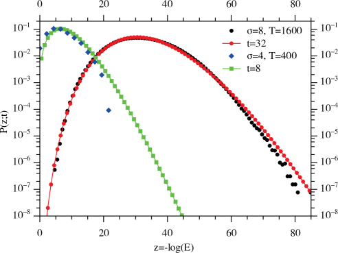
Figure 1: Size distributions obtained numerically for $p=0.01$, after $T=400$ iterations ($\sigma=4$) (squares) and after $T=1600$ iterations ($\sigma=8$) (circles). Lines with symbols represent the corresponding analytical results in (11), at $t=8$ and $32$.

Numerically, we performed simulations of the iterative process for give fragmentation probability $p$, starting from a single element of unit size, until a sufficient number of fragments was produced in $T$ iterations, and computed their size distribution. Since each iteration is performed in time interval $\Delta t$, the total elapsed time is given by $T\Delta t$. Recalling that $t$ represents the dimensionless time, measured in units of $(2\omega)^{-1}$, we thus have $T\Delta t=t/2\omega$ or $t=2pT$, relating $T$ and $t$. Accordingly, the deviation after $T$ iterations takes the value $\sigma=\sqrt{4pT}$. In Fig. 1, the distributions obtained numerically for two different values of $T$ are compared with the analytical distribution in (11) for the corresponding time $t\,(=2pT)$ . It is observed that the numerical data coincide with the analytical results except for large values of $z$, where there arise deviations probably due to the limited number of intervals in the region. Indeed such deviations tend to reduce as $T$ is increased. Note that the mean number of elements produced in $T$ iterations is given by $\langle n\rangle_{T}=(1+p)^{T}$ and the variance $\langle n^{2}\rangle_{T}-\langle n\rangle_{T}^{2}=(1-p)/(1+p)\langle n\rangle_{T}^{2}$ [18], which indicates that for small $p$ the number of elements fluctuates strongly, with the fluctuations of order of the number of elements produced. This can be explained with the Galton-Watson theory [19], from the generating function $g_{T}(z)=\sum_{n=1}^{2^{T}}z^{n}f_{T}(n)$, where $f_{T}(n)$ is the probability that at time $T$ there are $n$ elements of various (indistinct) sizes. The generating function satisfies the functional relation $g_{T+1}(z)=(1-p)g_{T}(z)+pg^{2}_{T}(z)$, from which we can deduce the moments corresponding to the number of fragments produced randomly. For example, we have $\langle n\rangle_{T}=\partial g_{T}(z)/\partial z|_{z=1}$. Although the number of elements fluctuates strongly, the size distribution is convergent to the well-defined distribution $P(z;t)$, even with only a small number of elements produced in a few time iterations, e.g., $\langle n\rangle_{T}\approx 53$ for $T=400$, as shown in Fig. 1.

2.4 Presence of a source

When a source is present ($r\neq 0$), the size distribution can still be obtained from (7), with the characteristic function $G(x;t)$ given by (6). It is useful to notice that the time derivative of the term proportional to $r$, $G_{1}(x;t)\equiv G(x;t)-G_{0}(x;t)$, is given by $\partial G_{1}(x;t)/\partial t=rG_{0}(x;t)$. This reveals that the contribution of $G_{1}$ in (7) is equal to that of $G_{0}$ integrated over time $t$ and multiplied by $r$. As a result, the size distribution is given by the sum of (11) and its integral, and consists in three terms:

$$P(z;t) = \rme^{-t}\delta(z)+\rme^{-t-z}\sqrt{\frac{t}{z}}\,I_{1}(2\sqrt{zt})++r\int_{0}^{t}d\tau\,\left[\rme^{-t}\delta(z)+\rme^{-z-\tau}\sqrt{\frac{\tau}{z}}I_{1}(2\sqrt{z\tau})\right]$$

$$= \left[r+(1-r)\rme^{-t}\right]\delta(z)+\rme^{-t-z}\sqrt{\frac{t}{z}}I_{1}(2\sqrt{zt})+\frac{r}{4z^{2}}\int_{0}^{2\sqrt{zt}}du\,u^{2}\,\exp\left(-z-\frac{u^{2}}{4z}\right)I_{1}(u),$$

where $\tau$ has been replaced by $u\equiv 2\sqrt{z\tau}$ in obtaining the last integral. In the large time limit, the first term in (2.4) coming from the source contributions reduces to $r\,\delta(z)$, whereas the second term becomes negligible. The resulting distributions for the production rate $r=1$ at time $t=1,5,10,$ and $20$ are displayed in Fig. 2. It is observed that a front wave develops with time, as the source introduces more unit size elements in the system. This front is located approximately at $z\approx t$.

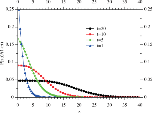
Figure 2: Size distribution normalized by the growth factor $(1+rt)$, with the production rate $r=1$ at different times. The distribution becomes flat for small sizes up to $z\approx t$, where the front is located.

3 General fragmentation rate

We now consider the possibility that each interval element is allowed to be fragmented into an arbitrary number of pieces, i.e., two (with probability $p_{2}$), three (probability $p_{3}$), or $n$ (probability $p_{n}$) pieces, with $\sum_{n=2}^{\infty}p_{n}=1$. In general, one can show that the generating function $G(x;t)$ satisfies a differential equation $\partial G(x;t)/\partial t=Q(x)G(x;t)+r$, with $Q(x)$ a rational function of $x$ having poles at positive integers on the real axis. The general evolution equation for $P(E;t)$ can be written with the help of the probability $(n-1)(E^{\prime}-E)^{n-2}/E^{\prime n-1}$ that an interval of size $E^{\prime}$ breaks into $n$ elements with one of given size $E\,(<E^{\prime})$; this may be confirmed by integrating successively over all possible sizes. Note that this probability is uniform only for $n=2$. Similarly to the case of binary fragmentation, the extended evolution equation reads

$$\frac{\partial P(E;t)}{\partial t}=-P(E;t)+\sum_{n=2}^{\infty}p_{n}(n-1)\int_{E}^{1}\frac{(E^{\prime}-E)^{n-2}}{E^{\prime n-1}}P(E^{\prime};t)\,dE^{\prime}+r\delta(E-1),$$ (15)

which, upon letting $E\equiv\rme^{-z}$ and changing the variable from $E$ to $z$, takes the form

$$\frac{\partial P(z;t)}{\partial t} = -P(z;t)+\sum_{m=2}^{\infty}p_{m}(m-1)\int_{0}^{z}dz^{\prime}\rme^{-z+(m-1)z^{\prime}}(\rme^{-z^{\prime}}-\rme^{-z})^{m-2}P(z^{\prime};t)$$ (16)

$$+ r\delta(z).$$

Multiplying both sides by $z^{n}$ and integrating over $z$, we obtain the evolution equations for the moments $M_{n}$ (or $R_{n}$). Specifically, we expand the term $(\rme^{-z^{\prime}}-\rme^{-z})^{m-2}$ by mean of the binomial formula and perform the integration by parts, to obtain

$$\frac{\partial R_{n}(t)}{\partial t}=-R_{n}(t)+\sum_{k=0}^{n}Q_{n-k}R_{k}(t)+r\delta_{n,0},$$ (17)

where $Q_{n-k}\equiv\sum_{m=2}^{\infty}(m-1)p_{m}\sum_{l=0}^{m-2}(-1)^{l}(l+1)^{-(n-k+1)}C_{m-2}^{l}$, and $Q_{0}=1$. This differential equation can be solved with the help of the generating function $G(x;t)$ defined previously. Equation (17) then leads to

$$\frac{\partial G(x;t)}{\partial t}=-G(x;t)+\sum_{n=0}^{\infty}x^{n}\sum_{k=0}^{n}Q_{n-k}R_{k}+r=Q(x)G(x;t)+r,$$ (18)

where the double sum in $Q_{n-k}$ has been rearranged to give

$$Q(x)\equiv\sum_{n=0}^{\infty}x^{n}Q_{n}-1=-1+\sum_{k=2}^{\infty}(k-1)p_{k}\sum_{l=0}^{k-2}\frac{(-1)^{l}C_{k-2}^{l}}{l+1-x}.$$ (19)

In the case of non-vanishing probabilities $p_{k}$ for $2\leq k\leq n+1$, $Q(x)$ is a rational function with simple poles located at $x=1,\cdots,n$. Note that when only $p_{2}$ is non-zero, (18), together with (19), reduces to (5) for the binary fragmentation process.

As before, the size distribution function can be evaluated from (7), where the generating or characteristic function is given by the solution of (18):

$$G(x;t)=\rme^{Q(x)t}-\frac{r}{Q(x)}\left[1-\rme^{Q(x)t}\right].$$ (20)

In the limit $x\rightarrow 0$, we have $G(0;t)\rightarrow 1+rt$ and the system grows with the scale factor $1{+}rt$, as expected. Here $Q(x)$ can also be rewritten in terms of an integral by exponentiating $(l+1-x)^{-1}$ in (19) and performing the sum over $k$:

$$Q(x)=-1+\int_{0}^{1}d\,u\,u^{-x}\sum_{k=2}^{\infty}(k-1)p_{k}(1-u)^{k-2}.$$ (21)

One can evaluate this integral precisely, performing successive integrations by parts, particularly by differentiating $(1-u)^{k-2}$ and using the formula $\int_{0}^{1}du\,(1-u)^{k}u^{-x}=k!\prod_{l=1}^{k+1}(l-x)^{-1}$. We thus obtain

$$Q(x)=-1+\sum_{k=2}^{\infty}p_{k}\frac{\Gamma(1{-}x)\Gamma(k)}{\Gamma(k{-}x)}=-1+\sum_{k=2}^{\infty}\frac{p_{k}}{\prod_{m=1}^{k-1}(1-x/m)},$$ (22)

which shows that the poles of $Q(-i\lambda)$ are located on the imaginary axis, at values $\lambda=in$ with integer $n\geq 1$.

Deforming the integration path in (7) near the first pole $\lambda=i$, we obtain an estimate for the saddle point value by writing $\lambda=iu$ with $u>0$ and considering the series expansion of $Q$ near $u=1$: $Q(u)\approx(1-u)^{-1}\sum_{k=2}^{\infty}(k-1)p_{k}$. Then the argument function $\varphi(u)=-uz+tQ(u)$ (henceforth in the absence of a source) has a saddle point solution equal to $u^{*}=1-\sqrt{(\kappa-1)t/z}$, where $\kappa=\sum_{k=2}^{\infty}kp_{k}$ is the mean number of fragments produced after breaking one interval element. When $\kappa$ is finite, we obtain the asymptotic solution of $P(z;t)$ for large $z$:

$$P(z;t) \approx \frac{(\kappa{-}1)^{1/4}}{2\sqrt{\pi}}\frac{t^{1/4}}{z^{3/4}}\exp\left[-z+2\sqrt{(\kappa{-}1)zt}-t\right].$$ (23)

Note that taking $p_{2}=1$ and $\kappa=2$, we recover (13) for binary fragmentation.

To be specific, we consider the case that the multiple fragmentation probabilities follow a power-law distribution: $p_{k}=[\zeta(1{+}\eta)]^{-1}(k-1)^{-1-\eta}$ with $\eta$ positive and the zeta function $\zeta(1{+}\eta)$ giving the normalization factor. Then the mean number of fragments is given by $\kappa=1+\zeta(\eta)[\zeta(1{+}\eta)]^{-1}$, which is finite for $\eta>1$. In this case, $Q(u)$ is approximated by

$$Q(u)\approx-1+\frac{\zeta(\eta)}{\zeta(1{+}\eta)}\left[\gamma+\frac{1}{1-u}\right]$$ (24)

with the Euler constant $\gamma$, for which the saddle point value is given by $u^{*}=1-\sqrt{\zeta(\eta)[\zeta(1{+}\eta)]^{-1}(t/z)}$. This leads to the distribution in the form:

$$P(z;t) \approx \frac{[\zeta(\eta)]^{1/4}}{2\sqrt{\pi}[\zeta(1{+}\eta)]^{1/4}}\frac{t^{1/4}}{z^{3/4}}\exp\left[-z+2\sqrt{\frac{\zeta(\eta)}{\zeta(1{+}\eta)}zt}-t-\frac{\gamma\zeta(\eta)}{\zeta(1{+}\eta)}t\right],$$ (25)

which is valid for $\eta>1$. The dominant contribution is given by the exponential decay $\rme^{-z}$, similarly to the previous binary fragmentation process.

When $0<\eta<1$, on the other hand, $\kappa$ becomes infinite, invalidating (25) based on (23). In this case it is convenient to rewrite (22) as

$$Q(u)=-1+\frac{1}{\zeta(1{+}\eta)}\sum_{k=1}^{\infty}\frac{\exp[\theta_{k}(u)]}{k^{1+\eta-u}}$$ (26)

with the argument

$$\theta_{k}(u)=-\sum_{m=1}^{k}\left[\log\Big{(}1-\frac{u}{m}\Big{)}+\frac{u}{m}\right]+u\left[\sum_{m=1}^{k}\frac{1}{m}-\log k\right].$$ (27)

In the limit of large $k$, function $\theta_{k}(u)$ approaches rapidly the well-defined finite limit: $\theta(u)=\log\Gamma(1{-}u)$. However, when $u$ approaches the value $\eta$, the sum of $k^{-1-\eta+u}$ diverges before $u$ reaches the pole of the $\Gamma$ function, $u=1$, changing the position of the saddle point value. It is then convenient to approximate $Q$ near $u=\eta$ by

$$Q(u)\approx-1+\frac{\Gamma(1{-}u)}{\zeta(1{+}\eta)}\zeta(1{+}\eta{-}u)\approx-1+\frac{\Gamma(1{-}u)}{\zeta(1{+}\eta)}\left[\frac{1}{\eta-u}+\gamma-\gamma_{1}(\eta{-}u)\right],$$ (28)

where $\gamma_{1}$ is the Stieltjes constant. The saddle-point solution $u^{*}$, obtained by deriving the argument function $\varphi(u)$ and solving $\partial\varphi(u)/\partial u=0$, leads accurately to the saddle-point value satisfied by the quadratic equation

$$\frac{\Gamma(1{-}\eta)t}{\zeta(1{-}\eta)(\eta-u^{*})^{2}}=z-C_{\eta}t,$$ (29)

where

$$C_{\eta}=\frac{\Gamma(1{-}\eta)}{\zeta(1{-}\eta)}\left[\gamma_{1}-\Psi(1{-}\eta)\gamma-\frac{1}{2}\Psi^{\prime}(1{-}\eta)-\frac{1}{2}\Psi(1{-}\eta)^{2}\right]$$ (30)

with $\Psi(x)\equiv d\log\Gamma(x)/dx$. There are two solutions and the correct one corresponds to $u^{*}<\eta$ or

$$u^{*}\approx\eta-\sqrt{\frac{\Gamma(1{-}\eta)t}{\zeta(1{+}\eta)(z-C_{\eta}t)}}$$ (31)

since deforming the path of integration starting from the real $\lambda$-axis to $\lambda=iu$ with $u>0$ is possible without crossing the singularity $u=\eta$ only if $u<\eta$ is satisfied. Expanding $\varphi(u)$ up to the second order in $u$ around $u^{*}$ and integrating the local Gaussian leads to the asymptotic estimate of $P(z;t)$ in the limit of large $z$, with $C_{\eta}t$ neglected:

$$P(z;t) \approx \frac{[\Gamma(1{-}\eta)]^{1/4}}{2\sqrt{\pi}[\zeta(1{+}\eta)]^{1/4}}\frac{t^{1/4}}{z^{3/4}}\exp\left[-\eta z+2\sqrt{\frac{\Gamma(1{-}\eta)}{\zeta(1{+}\eta)}zt}-t\right.$$ (32)

$$+ \left.\frac{\Gamma(1{-}\eta)}{\zeta(1{+}\eta)}\left[\gamma+\Psi(1{-}\eta)\right]t\right],$$

which is valid for $\eta<1$.

Comparing (25) and (32), we notice that for $\eta<1$ the dominant exponential decay coefficient is governed by $\eta$ rather than unity in the case $\eta\geq 1$ for which the saddle-point solution is always given by $\lambda=i$ independently of $\eta$. Corrective terms are proportional to $\sqrt{z}$ in the exponential argument, with the difference that $\zeta(\eta)$ for $\eta>1$ is replaced by $\Gamma(1{-}\eta)$ when $\eta<1$. Otherwise, the logarithmic correction has the same factor $3/4$ in both cases. The asymptotic formulae given by (25) and (32) are verified with numerical integration of (20), as displayed in Fig. 3 for $\eta=2$ and $\eta=0.5$.

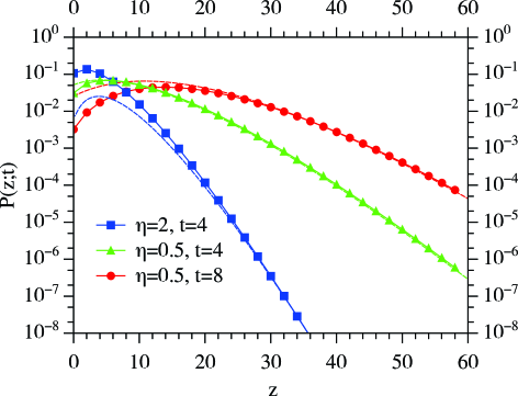
Figure 3: Size distribution in the absence of a source with the power-law distribution $p_{k}\propto k^{-1-\eta}$ of the number of elements produced after one fragmentation. Dashed lines represent the asymptotic results based on (32) for $\eta<1$ and (25) for $\eta>1$, respectively, by means of the saddle-point approximation and path deformation in the integral of (20) near $\lambda=i$ for the first case and $\lambda=i\eta$ for the second one.

The case $\eta=1$ is special and needs a separate treatment. For this, we can express $Q(u)$ in terms of the $\Gamma$ functions:

$$Q(u)=-1+\frac{6}{\pi^{2}}\left[\Psi^{\prime}(-u)-\frac{1}{u^{2}}\right].$$ (33)

Near the singular value $u=1$, we can expand the argument function $\varphi(u)$ and obtain the saddle-point solution: $u^{*}\approx 1-[\pi^{2}z/(12t)-\zeta(3)]^{-1/3}$. It is clear that $1-u^{*}$ scales as $z^{-1/3}$ instead of $z^{-1/2}$ and that this solution gives a dominant term in $\rme^{-z}$ and corrections which have different behavior from the previous cases. Specifically, the size distribution takes the form

$$P(z;t)\approx\frac{2^{1/6}}{3^{1/3}\pi^{5/6}}\frac{t^{1/6}}{z^{2/3}}\exp\left[-z+\frac{3^{4/3}}{2^{1/3}\pi^{2/3}}z^{2/3}t^{1/3}\right]$$ (34)

for $\eta=1$.

4 Discussion

We have studied the general fragmentation process, in which each existing element of size $E$ can be fragmented into $k$ elements with probability $p_{k}$. The evolution equation for the size distribution function $P(E;t)$ has been built and solved to yield $P(E;t)$ in the presence/absence of a source term producing elements of unit size. Different cases have been probed, in particular when the probability of breaking an element into $k$ elements follows a power law: $p_{k}\propto k^{-1-\eta}$. The asymptotic behavior of $P(E;t)$ for small $E$ has been obtained according to the value of $\eta$.

In terms of the distribution $P(E;t)$ in the limit of small $E\,(\ll 1)$, the results are summaried as follows: For $\eta>1$, the distribution is asymptotically given by $P(E;t)\propto\exp[\sqrt{-\alpha t\log E}](-\log E)^{-3/4}$ with $\alpha=4\zeta(\eta)/\zeta(1{+}\eta)$, whereas for $\eta<1$, we have $P(E;t)\propto E^{\eta-1}\exp(\sqrt{-\alpha t\log E})(-\log E)^{-3/4}$ with $\alpha=4\Gamma(1{-}\eta)/\zeta(1{+}\eta)$. For $\eta=1$, on the other hand, we obtain $P(E;t)\propto\exp[(\alpha t\log^{2}E)^{1/3}](-\log E)^{-2/3}$ with $\alpha=27/[4\zeta(2)]$. The asymptotic regime is thus dominated in general by whether $\eta$ is larger/smaller than unity or whether the mean number $\kappa$ of fragments is finite. It also depends on the location of the saddle point, relatively to the first pole of the $\Gamma$ function, $\lambda=i$. In the special case $\eta=1$, we have obtained the exact expression of the argument function $\varphi$ and treated accurately the saddle-point value which differs from that in other cases. In view of classic models of fragmentation, these results differ from Moot-Linfoot [7, 20] in the fact that variable $E$ in the stretched exponential is replaced by $-\log E$ and that other corrections are present. Generalization to more realistic cases is possible here, for example when distributions $p_{k}$ depend statistically on the interval length $E$ and decrease as $E$ becomes smaller (i.e. fragmentation becomes less effective when fragments are too small down to an intrinsic length of the system), and this can be studied using generating function (20) and (22).

References

References

• [1] Brown W, Karpp R and Grady D 1983 Astrophysics and Space Science 94(2) 401–412 ISSN 0004-640X URL http://dx.doi.org/10.1007/BF00653729
• [2] Holian BΒ L and Grady DΒ E 1988 Phys. Rev. Lett. 60(14) 1355–1358 URL http://link.aps.org/doi/10.1103/PhysRevLett.60.1355
• [3] Brown WΒ K 1989 J. Astrophys. Astr. 10 89–112
• [4] Ziff RΒ M and McGrady EΒ D 1986 Macromolecules 19 2513–2519
• [5] Derrida B and Flyvbjerg H 1987 J. Phys. A: Math. Gen. 20 5273–5288
• [6] Mott N and Linfoot E 1943 A theory of fragmentation Tech. Rep. AC3348 United Kingdom Ministry of Supply
• [7] Grady DΒ E and Kipp MΒ E 1985 Journal of Applied Physics 58 1210–1222 URL http://link.aip.org/link/?JAP/58/1210/1
• [8] Choi MΒ Y, Choi H, Fortin JΒ Y and Choi J 2009 EPL (Europhysics Letters) 85 30006
• [9] Goh S, Kwon HΒ W, Choi MΒ Y and Fortin JΒ Y 2010 Phys. Rev. E 82(6) 061115 URL http://link.aps.org/doi/10.1103/PhysRevE.82.061115
• [10] Yule GΒ U 1925 Philos. Trans. R. Soc. London Ser. B 213
• [11] Ziff RΒ M and McGrady EΒ D 1985 Journal of Physics A: Mathematical and General 18 3027
• [12] Hassan M and Rodgers G 1995 Physics Letters A 95–98
• [13] Krapivsky PΒ L, Grosse I and Ben-Naim E 2000 Phys. Rev. E 61 R993
• [14] Dean DΒ S and Majumdar SΒ N 2002 Journal of Physics A: Mathematical and General 35 L501 URL http://stacks.iop.org/0305-4470/35/i=32/a=101
• [15] Krapivsky PΒ L, Ben-Naim E and Grosse I 2004 J. Phys. A: Math. Gen. 37 2863–2880
• [16] Athreya KΒ B and Ney PΒ E 1972 Branching processes (New York: Springer-Verlag)
• [17] Grady DΒ E 1990 Journal of Applied Physics 68 6099–6105 URL http://link.aip.org/link/?JAP/68/6099/1
• [18] Jo J, Fortin JΒ Y and Choi MΒ Y 2011 Phys. Rev. E 83(3) 031123 URL http://link.aps.org/doi/10.1103/PhysRevE.83.031123
• [19] Seneta E 1969 Adv. Appl. Prob. 1 1–42
• [20] Levy S 2010 Exploring the Physics behind Dynamic Fragmentation through Parallel Simulations Ph.D. thesis Γ‰cole Polytechnique FΓ©dΓ©rale de Lausanne