Cluster mean-field theory study of $J_{1}-J_{2}$ Heisenberg model on a square lattice

Abstract

We study the spin-$1/2$ $J_{1}$-$J_{2}$ Heisenberg model on a square lattice using the cluster mean-field theory. We find a rapid convergence of phase boundaries with increasing cluster size. By extrapolating the cluster size $L$ to infinity, we obtain accurate phase boundaries $J_{2}^{c1}\approx 0.42$ (between the N$\acute{e}$el antiferromagnetic phase and nonmagnetic phase), and $J_{2}^{c2}\approx 0.59$ (between nonmagnetic phase and the collinear antiferromagnetic phase). The transitions are identified unambiguously as second order at $J_{2}^{c1}$ and first order at $J_{2}^{c2}$. At finite temperature, we present a complete phase diagram with stable, meta-stable and unstable states near $J_{2}^{c2}$, being relevant to that of the anisotropic $J_{1}-J_{2}$ model. The uniform as well as staggered magnetic susceptibilities are also discussed.

Keywords $J_{1}-J_{2}$ Heisenberg model, quantum phase transition, cluster mean-field theory

1 Introduction

It was suggested by P. W. Anderson[1] that low spin, low spatial dimension, and high frustration are the three main factors which favor the melting of magnetic long range order (LRO) and lead to exotic spin liquid ground state. Such a state was closely related to the appearance of superconductivity in the high-temperature superconductivity in Cu-based oxides upon doping[2]. The spin-$1/2$ $J_{1}$-$J_{2}$ Heisenberg model in two dimensional square lattice is such a model that bears all the three factors, hence its ground state is a promising candidate for the exotic spin liquid state[3]. Besides the interest for spin liquid, this model in the large $J_{2}/J_{1}$ regime is relevant to materials such as $Li_{2}VOSiO_{4}$[4], and the $S>1/2$ version is relevant to the parent material of iron-based high temperature superconductors[5].

The Hamiltonian of antiferromagnetic (AFM) $J_{1}-J_{2}$ model reads

$$\hat{H}=J_{1}\sum_{\langle i,j\rangle}\mathbf{S}_{i}\cdot\mathbf{S}_{j}+J_{2}\sum_{\langle\langle i,j\rangle\rangle}\mathbf{S}_{i}\cdot\mathbf{S}_{j},$$ (1)

where $\mathbf{S_{i}}$ is the spin $\frac{1}{2}$ operator on site $i$, $J_{1}$ and $J_{2}$ are the nearest neighbor and the next-nearest neighbor coupling coefficients, respectively. In the following, we set $J_{1}=1$ as the unit of energy. For the next-nearest neighbor coupling $J_{2}$, we confine ourself to the AFM case $J_{2}>0$.

This model received numerous studies in the past two decades, using various methods including exact diagonalization (ED)[6, 7, 8, 9, 10], series expansion[11, 12, 13, 14, 15], coupled cluster[16, 17], spin wave approximation[3, 18], Green’s function method[19], density-matrix renormalization group (DMRG)[20], matrix-product or tensor-network based algorithms[21, 22, 23, 24], high temperature expansion[25], resonating valence bond approaches[26, 27, 28, 29], exact solution[30], bond operator formalism[31, 32], mean-field theories[11, 33, 34], and field theoretical methods[35, 36, 37]. It has been established that in the regime $0<J_{2}/J_{1}\lesssim 0.4$, the ground state of $J_{1}-J_{2}$ model is an AFM phase with N$\acute{e}$el order. In $J_{2}/J_{1}\gtrsim 0.6$, an AFM phase with collinear LRO is stable, due to the dominance of the next-nearest-neighbor coupling $J_{2}$. One of the most controversial regime is the intermediate regime $0.4\lesssim J_{2}/J_{1}\lesssim 0.6$ where the ground state is non-magnetic and hence the SU(2) symmetry is not broken. The nature of this intermediate non-magnetic ground state is still a much debated issue. The possible candidates of this ground state, as been proposed by various authors, include dimerized valence bond solid (VBS) which breaks both the translation and the rotation symmetries of the lattice[7, 11, 12, 13], the plaquette VBS which breaks only the translation symmetry[31, 36, 34], the nematic spin liquid which breaks only the rotational symmetry[37], and the gapped[20, 24, 27] or gapless[29] spin liquid which conserves all the symmetries of the lattice. The difficulty of this issue lies in that there is no unbiased and accurate method to study the ground state of $J_{1}-J_{2}$ model in the thermodynamical limit. Most of the numerical studies heavily rely on the extrapolation of the finite size results to the thermodynamical limit. In cases where there is little guide from the analytical knowledge, this practice may have uncertainties[38, 22] as demonstrated by a recent study on the J-Q model[39].

Besides the nature of the nonmagnetic state, there are other important issues under various physical contexts. Previous studies show that AFM N$\acute{e}$el phase transits into the non-magnetic state at $J_{2}/J_{1}\approx 0.4$ through a continuous quantum phase transition. If the intermediate region actually possesses a VBS order, this transition is an abnormal one, as a continuous transition between two phases without the group-subgroup symmetries violates the conventional ”Landau rule”. A ”deconfined” quantum critical point was proposed to exist between the N$\acute{e}el$ and the VBS states[40].

For the parameter regime $J_{2}/J_{1}\gtrsim 0.6$, this model also invoked much interest since lots of real materials are related to this parameter regime, such as the La-O-Cu-As iron based superconductors[41, 42] and $Li_{2}VOSiO_{4}$[4]. Another interesting issue in this parameter regime is the possible finite temperature symmetry breaking. For this model, although the spin SU(2) symmetry cannot be broken spontaneously at finite temperature due to the Mermin-Wagner theorem[43], symmetry breaking of the lattice $C_{4}$ symmetry could occur below a finite $T<T_{c}$[35, 44, 45]. However, there is also a different opinion on this issue[14].

The effect of spin-anisotropy in the $J_{1}-J_{2}$ model is also an interesting issue, given that the anisotropy is quite common in real materials. Theoretical studies on this issue is rare[46, 47].

In this paper, we focus on the phase boundary of the the $J_{1}-J_{2}$ model and attempt to present accurate critical values $J_{2}^{c1}$ and $J_{2}^{c2}$. We use the cluster mean-field theory (CMFT), which is the cluster extension of the Weiss mean-field theory[48, 49]. We obtained the N$\acute{e}$el AFM phase, the collinear AFM phase, and the nonmagnetic phase. Using the reshaping method for plotting multiple-valued curves[50], we studied the fine structure of the first order phase transition between the nonmagnetic phase and the collinear AFM phases, including the stable, meta-stable and unstable phases. These informations are important when the system is under external influence but are often neglected in previous studies. The critical values $J_{2}^{c1}$ and $J_{2}^{c2}$ are found to converge very fast with increasing cluster size, allowing us to obtain an accurate estimation of them. We also analyze the finite temperature properties, the mean-field results for which, though incorrect for the isotropic model itself, are known to be relevant to the corresponding properties of the anisotropic $J_{1}-J_{2}$ model.

The rest part of this paper is organized as follows: In Sec. II, we introduce the CMFT and the method we used to obtain the fine structure of the first-order phase transition. In Sec. III, we first present the zero temperature results in part A, including the phase diagram and magnetic susceptibility. In part B, a phase diagram at finite temperature is given and various susceptibilities are presented and discussed.

2 Method

The simplest mean-field theory for spin systems is the Weiss’s single-site mean-field theory[48]. In this theory, the influence of surrounding spins to a central spin is approximated by an effective static field, which is then determined self-consistently. The Weiss mean-field theory thus neglects the spatial fluctuations and often overestimates the stability of LRO. Based on a similar idea, Bethe-Peierls-Weiss (BPW)[52, 53, 54] and Oguchi[55] improved the approximation by mapping the lattice model into clusters subjected to self-consistently determined effective fields. The interactions inside a cluster is treated exactly while interactions between clusters are approximated by mean fields. Since the short-range spatial fluctuations inside a cluster are taken into account, the results are expected to improve as cluster size increases.

In this work, we study the $J_{1}-J_{2}$ model on a square lattice using the cluster extension of Weiss mean-field theory. Although being simple, this theory produces surprisingly accurate boundaries between various phases, as compared to results from more sophisticated methods. We first divide the lattice into identical clusters of $L$ sites. To separate the spin couplings inside a cluster from those between clusters, the Hamiltonian of $J_{1}-J_{2}$ model is rewritten as

$$\hat{H} = \sum_{c_{n}}\left[J_{1}\sum_{\langle ij\rangle}\mathbf{S}_{i,c_{n}}\cdot\mathbf{S}_{j,c_{n}}+J_{2}\sum_{\langle\langle ij\rangle\rangle}\mathbf{S}_{i,c_{n}}\cdot\mathbf{S}_{j,c_{n}}\right]$$

$$+ \sum_{c_{n}\neq c_{m}}\left[J_{1}\sum_{\langle ij\rangle}\mathbf{S}_{i,c_{n}}\cdot\mathbf{S}_{j,c_{m}}+J_{2}\sum_{\langle\langle ij\rangle\rangle}\mathbf{S}_{i,c_{n}}\cdot\mathbf{S}_{j,c_{m}}\right].$$

The operator $S_{i,c_{n}}$ donates the spin operator on the $i$-th site in the cluster $c_{n}$. The first term in Eq.(2) represents the Hamiltonian of decoupled clusters, while the second one represents interactions between clusters. We make the standard mean-field approximation for the interactions between two spins belonging to different clusters $c_{n}\neq c_{m}$,

$$\mathbf{S}_{i,c_{n}}\cdot\mathbf{S}_{j,c_{m}}\approx S^{z}_{i,c_{n}}\langle S^{z}_{j,c_{m}}\rangle+\langle S^{z}_{i,c_{n}}\rangle S^{z}_{j,c_{m}}-\langle S^{z}_{i,c_{n}}\rangle\langle S^{z}_{j,c_{m}}\rangle.$$ (3)

Here, $z$-axis is chosen as the quantization axis. This approximation breaks both spin SU(2) symmetry and spatial translation symmetry of the original Hamiltonian. Substituting it into the second term of Eq.(2) and neglecting a constant, we obtain the cluster-decoupled mean-field Hamiltonian,

$$\hat{H}_{mf} = \sum_{c_{n}}\hat{H}_{c_{n}}$$

$$\hat{H}_{c_{n}} = J_{1}\sum_{\langle ij\rangle}\mathbf{S}_{i,c_{n}}\cdot\mathbf{S}_{j,c_{n}}+J_{2}\sum_{\langle\langle ij\rangle\rangle}\mathbf{S}_{i,c_{n}}\cdot\mathbf{S}_{j,c_{n}}$$ (4)

$$+\sum_{i=1}^{L}h_{i}S^{z}_{i,c_{n}}.$$

Here $h_{i}$ is the effective static field felt by the spin $\mathbf{S}_{i,c_{n}}$. It is a linear combination of ${\langle S^{z}_{j,c_{m}}\rangle}$, the magnetization of boundary site $j$ on the neighboring cluster $c_{m}$.

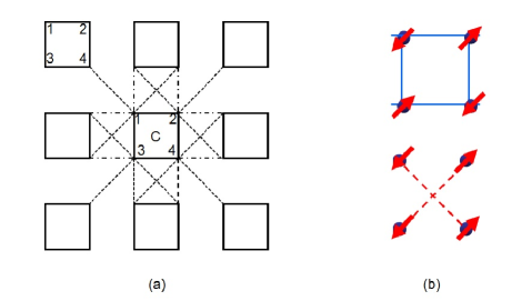
Figure 1: (a) The square lattice is divided into $2\times 2$ clusters (solid lines). The interactions between different clusters are denoted by dot-dashed lines ($J_{1}$) and dashed lines ($J_{2}$). (b) Upper: picture of N$\acute{e}$el AFM order, dominated by the nearest antiferromagnetic interaction $J_{1}$ (solid lines). Lower: picture of collinear AFM order, dominated by the next nearest antiferromagnetic interaction $J_{2}$ (dashed lines).

Fig.1 shows an example of $2\times 2$ clusters and their couplings between each other. We use the spatial translation symmetry of clusters to ensure $\langle S^{z}_{i,c_{n}}\rangle=\langle S^{z}_{i}\rangle=m_{i}$. For a cluster with $L$ sites, $m_{i}$ ($i=1,2,...,L$) are our magnetic order parameters that can characterize different magnetic orders. In this paper, we do not consider the possibility of LRO in the intermediate non-magnetic regime, as it is still an open issue how to incorporate the non-magnetic order parameters into the CMFT. With this notation, the effective field ${h_{i}}$ reads

$$h_{i}=J_{1}\sum_{\delta}m_{\delta}+J_{2}\sum_{\delta^{\prime}}m_{\delta^{\prime}}.$$ (5)

Here $\delta$, $\delta^{\prime}$ $\in[1,L]$, denoting the nearest neighbor site and the next-nearest neighbor site in the neighboring clusters of site i, respectively. The CMFT equations are completed by solving $m_{i}$ from a central cluster Hamiltonian $\hat{H}_{c}$ in Eq.(4). In the limit of single-site cluster $L=1$, the above approximation recovers the Weiss mean-field theory. As the cluster size increases, longer and longer range correlations contained in the cluster are treated exactly. Therefore, the results are expected to become exact as $L$ tends to infinity.

To solve the CMFT equations, we use open boundary conditions for the cluster. The $L$ magnetization values $m_{i}$ ($i=1,2,...,L$) are solved independently without symmetry constraints. Due to the lack of translation symmetry within the cluster, $|m_{i}|$ has a weak site-dependence, being smaller on the center of the cluster, and larger on the edge and even larger at the corner. The qualitative behavior of magnetization on different sites are exactly the same, i.e. they will be zero or non-zero at the same time, indicting the appearance or disappearance of the magnetic LRO.

We use iterative method to solve the mean-field equations. For a given set of effective fields ${h_{i}}$, we use Lanczos method (for $T=0$) or full ED method (for $T>0$) to calculate the magnetization ${m_{i}}$ which are feed back to Eq.(5). This process iterates until all the $m_{i}$’s converge. For a given $J_{2}$ and $T$, the calculation starts from a initial set of $m_{i}$’s, which we usually get from the self-consistent solution of a slightly deviated parameter $J_{2}$ (or $T$). Thus we can scan the parameter space from small $J_{2}$ (or $T$) to larger values, or vice versa. It turns out that the set of mean-field equations has more than one solutions, stabilized respectively by scanning from left to right or from right to left along the $J_{2}$ (or $T$) axis. For those multiple solutions at a fixed ($J_{2}$, $T$), we compare their energies ($T=0$) or free energies ($T>0$) to determine the physical solution of this system. After the solutions of $m_{i}$ ($i=1,2,...,L$) are obtained, its LRO can be identified easily from the magnetization pattern.

Near $J_{2}\approx 0.6$, naive scanning of $J_{2}$ produces a discontinuous $m-J_{2}$ curve: $m$ jumps from $0$ to a finite value or vice versa ($m$ is the magnetization of a center site of the cluster). We suppose that this is the numerical instability due to the multiple-valued relation of $m-J_{2}$. If such structure does exist, ordinary calculation can only produce one branch of solution and neglect the others, leading to a jump at some $J_{2}$ where the relative stabilities of two solutions invert. To overcome this problem, we use the ”stretching trick” proposed in the study of first-order phase transitions in correlated electron systems[50]. If the mean-field solution $m=F(J_{2})$ is a continuous curve in the $m-J_{2}$ plane but has a $S$- or $Z$-shaped turn, the new equation $m=F(J_{2}-V|m|)$ will produce a single-valued $m-J_{2}$ curve, given a proper selection of $V>0$. Pictorially this single-valued curve is obtained by ”stretching” the original curve. We can then solve this modified equation first and recover the original solutions by plotting $m$ versus $J_{2}-V|m|$.

3 Results and Discussions

3.1 Zero Temperature

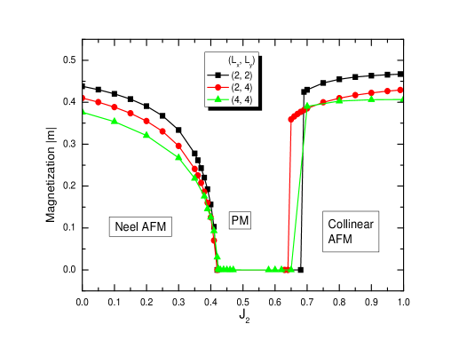
Figure 2: Magnetization $m$ versus $J_{2}$ obtained using various cluster geometries. The pattern of LRO’s are marked in the figure. PM denotes paramagnetic. Here $m$ is the magnetization of a spin at the center of the cluster.

In this work, we use the rectangular clusters of size $L=L_{x}\times L_{y}$. To avoid odd number of spins in a cluster, we use even $L_{x}$ and $L_{y}$. The total number of spins $L$ is confined as $L\leq 16$ due to the exponential increase of computational cost with $L$. We choose $2\times 2$ and $4\times 4$ clusters for qualitative study, and use $L_{y}=2$ and $L_{x}=2,4,6,8$ for quantitative size dependence analysis.

In Fig.2, we show $|m|$ versus $J_{2}$ for three successively larger clusters. $|m|$ is measured on the center site of the cluster. For all the clusters we used, the N$\acute{e}$el order is stable for small $J_{2}$ regime. As $J_{2}$ increases, $|m|$ decreases and vanishes continuously at a critical value $J_{2}^{c1}\approx 0.41-0.42$, which indicates a second order transition to a non-magnetic phase. As $J_{2}$ increases above $J_{2}^{c2}\approx 0.6-0.7$, $|m|$ jumps from zero to a finite value, with a collinear magnetic pattern. In both N$\acute{e}$el and collinear phases, $m$ decreases with increasing $L$, showing that more and more quantum fluctuations are taken into account by using large clusters, and hence the increasing quality of our results. The exact value $m=0.307$[51] for $J_{2}=0$ is only asymptotically approached in $L=\infty$ limit. It is interesting to observe that the critical point $J_{2}^{c1}$ does not change much from $L=4$ to $L=16$, showing that it converges very rapidly with $L$. Taking the $L=16$ result as out estimation for the thermodynamical limit, we obtain $J_{2}^{c1}\approx 0.42$. Compared to other methods such as the ED[7, 8], series expansion[11, 13] and DMRG[20], CMFT is surprisingly accurate and simple in producing the ground state phase boundaries.

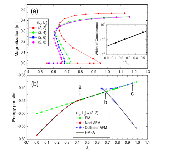
Figure 3: (a) Magnetization $|m|$ of a center spin versus $J_{2}$ near the first order phase transition for $L_{y}=2$ and $L_{x}=2$, $4$, $6$, and $8$, respectively. Inset: The width of coexistence region versus $1/L_{x}$. (b) Ground state energy per site versus $J_{2}$ in different phases, obtained using $L_{x}=L_{y}=2$ cluster. The arrows mark the second-order N$\acute{e}$el-to-nonmagnetic transition (arrow a), the first order nonmagnetic-to-collinear transitions (arrow b), and the meta-stable second-order nonmagnetic-to-collinear transition (arrow c). Symbols are data and the dashed lines are for guiding the eyes. The solid line is the result of Hierarchical mean-field approach using $2\times 2$ cluster in Ref.[34].

In Fig.3(a), we take a closer look at the fine structure of the $|m|-J_{2}$ curve near $J_{2}^{c2}$, where the transition between the non-magnetic phase and collinear AFM phase occurs. It is obtained by the ”stretching trick” mentioned above. In order to see the systematic cluster size dependence, we fix $L_{x}=2$ and increase $L_{y}$ from $2$ to $8$. We always obtain continuous curves with $S$-shaped structures which contain the stable, meta-stable, and the unstable phases and are generic features of the first order phase transition. The width of the coexistence region $W$ decreases as $L_{y}$ increases. As shown in the inset of Fig.3(a), $W$ is found to scale with $1/L_{y}$ as $W\propto\alpha e^{\beta/L_{y}}$ for the calculated cluster size. Fitting of the data gives $\alpha=0.038$ and $\beta=0.42$. $\alpha=0.038>0$ means that the first order phase transition still exists even if we use a cluster $L_{x}=2,L_{y}=\infty$. This seems to be a strong support to the first-order phase transition between non-magnetic phase and collinear AFM phase in the thermodynamical limit. For a more convincing conclusion, one should extrapolate $L_{x}$ and $L_{y}$ to infinity simultaneously. However, due to the rapid increase of the numerical cost, this is not done in our present study.

In Fig.3(b), the ground state energy per site versus $J_{2}$ is plotted for the N$\acute{e}$el AFM, non-magnetic, and the collinear AFM phases. We show the result obtained using $2\times 2$ cluster for demonstration purpose. As $J_{2}$ increases up to $0.42$ (marked by arrow ”a”), the energy of N$\acute{e}$el AFM continuously approaches that of the non-magnetic phase from below, consistent with the scenario of a second-order transition. The transition between the non-magnetic phase and the collinear AFM phase occurs at the energy crossing point marked by the arrow ”b” in Fig.3(b), which we denote as $J_{2}^{c2}$. In the coexistence region, a third collinear AFM solution has the highest energy. It corresponds to the unstable solution with negative $|m|-J_{2}$ slope in Fig.3(a). In this first-order transition, a continuous transition does exist at the meta-stable level, between collinear AFM and non-magnetic phases (marked by arrow ”c”).

This scenario is common in first order phase transitions described by mean-field equations, as disclosed by the dynamical mean-field theory study for the correlated electron systems[50]. Extrapolating $L_{y}$ to infinity, we get $J_{2}^{c2}\approx 0.59$, which should be very close to the exact value in the thermodynamical limit. This value agrees quite well with the more sophisticated calculations such as DMRG[20] (see Table.1 below). It is noted that our energy curve agree quantitatively with the result from the hierarchical mean-field approach (HMFA) on $2\times 2$ cluster[34] (solid lines in Fig.3(b)). Although HMFA is based on the sophisticated Schwinger boson representation and mean-field approximation, the quantitative agreement makes us believe that the HMFA is equivalent to the cluster mean-field method that we used here, at least for the case of $2\times 2$ cluster. The critical values of $J_{2}$ have been obtained in many works, using different methods with varied sophistications. In Table.1, we summarize some of the previous results and compare them with ours. Note that a similar CMFT study on the $J_{1}-J_{2}$ model was carried out in Ref.[11], but the cluster size effect was not analyzed systematically.

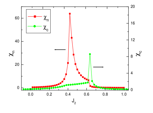
Figure 4: Zero temperature N$\acute{e}$el susceptibility $\chi_{n}$ (squares with guiding line) and collinear susceptibility $\chi_{c}$ (dots with guiding line) as functions of $J_{2}$. The data are obtained by numerical derivation with the applied field $h=0.01$.

Table 1: Comparison of $J_{2}^{c1}$ and $J_{2}^{c2}$ from various works. The methods are abbreviated as ED(exact diagonalization), SE(series expansion), DMRG(density-matrix renormalization group), HMFT(hierarchical mean-field theory), VMC(variational Monte Carlo), and CMFT(cluster mean-field theory).

Ref.	[8]	[11]	[20]	[17]	[34]	[29]	this work
Met.	ED	SE	DMRG	CC	HMFT	VMC	CMFT
$J_{2}^{c1}$	0.35	0.41	0.41	0.44	0.42	0.45	0.42
$J_{2}^{c2}$	0.66	0.64	0.62	0.59	0.66	0.6	0.59

A central issue in the study of $J_{1}-J_{2}$ model is the properties of the intermediate non-magnetic phase. The key question is whether it is a spin liquid or a VBS that breaks the lattice translation and/or rotation symmetry. Since in CMFT, the translation symmetry of the original lattice is broken by hand, we cannot answer this question directly. In the non-magnetic phase, the effective fields of CMFT become zero and $H_{mf}$ describes uncorrelated clusters. Then CMFT is equivalent to the bare ED on a cluster with open boundary condition, in contrast to periodic boundary condition commonly used in previous ED studies. The open boundary condition will induce nonzero VBS order parameter in small clusters. For an example, the operator of plaquette order parameter reads[56]

$$Q_{\alpha\beta\gamma\delta} = 2[(\mathbf{S}_{\alpha}\cdot\mathbf{S}_{\beta})(\mathbf{S}_{\gamma}\cdot\mathbf{S}_{\delta})+(\mathbf{S}_{\alpha}\cdot\mathbf{S}_{\delta})(\mathbf{S}_{\beta}\cdot\mathbf{S}_{\gamma})$$

$$-(\mathbf{S}_{\alpha}\cdot\mathbf{S}_{\gamma})(\mathbf{S}_{\beta}\cdot\mathbf{S}_{\delta})]+\frac{1}{2}(\mathbf{S}_{\alpha}\cdot\mathbf{S}_{\beta}+\mathbf{S}_{\gamma}\cdot\mathbf{S}_{\delta}$$

$$+\mathbf{S}_{\alpha}\cdot\mathbf{S}_{\delta}+\mathbf{S}_{\beta}\cdot\mathbf{S}_{\gamma}+\mathbf{S}_{\alpha}\cdot\mathbf{S}_{\gamma}+\mathbf{S}_{\beta}\cdot\mathbf{S}_{\delta}+\frac{1}{4}).$$

Here $\alpha,\beta,\gamma,\delta$ denote the four sites of a plaquette clockwise. At $J_{2}=0.5$, the plaquette order parameter is evaluated on a $2\times 2$ cluster as $Q_{\alpha\beta\gamma\delta}\thickapprox 0.988$, very close to its saturate value $1.0$. Evaluating $Q_{\alpha\beta\gamma\delta}$ on a larger cluster also gives nonzero result. However, these are the boundary effect of the cluster and does not support a true VBS state. It is an interesting open question how to incorporate the order parameter of various VBS state into the mean-field approximation. If such a mean-field theory does exist, considering that it tends to exaggerated the LRO, a negative result about the existence of VBS may rule out the possibility of VBS in the intermediate parameter regime.

We also investigate the N$\acute{e}$el as well as collinear magnetic susceptibility at zero temperature. These susceptibilities are defined as

$$\chi_{\alpha} = \displaystyle\lim_{h\rightarrow 0^{+}}\frac{Tr\left[e^{-\beta(\hat{H}-hM_{\alpha})}M_{\alpha}\right]}{Tr\left[e^{-\beta(\hat{H}-hM_{\alpha})}\right]}.$$ (7)

Here, the N$\acute{e}$el susceptibility $\chi_{n}$ and collinear susceptibility $\chi_{c}$ are defined using staggered magnetization $M_{n}$ and $M_{c}$, respectively. For the $2\times 2$ cluster shown in Fig.1, $M_{n}=S_{1}^{z}-S_{2}^{z}+S_{3}^{z}-S_{4}^{z}$ and $M_{c}=S_{1}^{z}+S_{2}^{z}-S_{3}^{z}-S_{4}^{z}$. We apply a small staggered field $h$ and evaluate $\chi_{n}$ and $\chi_{m}$ using numerical derivation. The results obtained are shown in Fig.4.

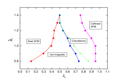
Figure 5: Phase diagram on the $\lambda-J_{2}$ plane obtained using $2\times 2$ cluster. Squares with solid line is the second-order transition between N$\acute{e}$el AFM and non-magnetic phases. Dots and diamonds with solid lines represent the phase coexistence boundary of non-magnetic phase and the collinear phase. The triangle with dashed line is the actual first-order phase transition line. The lines are for guiding eyes.

The continuously diverging behavior of $\chi_{n}$ at $J_{2}\approx 0.42$ confirms the continuous transition from N$\acute{e}$el AFM phase to non-magnetic phase. In contrast, near the collinear transition $J_{2}^{c2}$, an abrupt jump of $\chi_{c}$ is observed, being consistent with a first-order phase transition. Note that both $\chi_{n}$ and $\chi_{c}$ are much larger in the non-magnetic regime than in their corresponding long-ranged ordered regime. This shows that the intermediate non-magnetic ground state is rich of short range spin fluctuations at various momentums, and different types of spin correlation compete strongly with each other. This leads to the notorious difficulty in the study of the non-magnetic state.

The mean-field approximation used in our study introduces a symmetry breaking term $H^{\prime}=\sum_{i=1}^{L}h_{i}S^{z}_{i,c_{n}}$, which breaks the SU(2) symmetry of the original Hamiltonian. For CMFT calculation using a finite cluster, this term effectively suppresses the quantum fluctuation and tends to exaggerate the stability of LRO in the ground state. As a result, the obtained $|m|$ is larger than the exact value (as checked at $J_{2}=0$ case). The region of the magnetic LRO is enlarged and non-magnetic region suppressed. Here, to phenomenologically study the effects of enhancing or reducing quantum fluctuations, we introduce artificial fluctuations by multiplying a tunable factor $\lambda$ to the mean-field term $H^{\prime}$. The total Hamiltonian becomes $H_{eff}=H_{c_{n}}+\lambda H^{\prime}$. $\lambda<1$ enhances the fluctuation of $H_{eff}$, and it mimics the effects of larger cluster or smaller $S$. $\lambda>1$ reduces the fluctuation of $H_{eff}$ and it mimics the effects of anisotropy or larger spin. Fig.5 shows a phase diagram in $\lambda-J_{2}$ plane. For larger $\lambda$, the LRO region is enlarged and the non-magnetic region shrinks. At $\lambda=1.4$, non-magnetic region diminishes, leading to a direct first-order transition between N$\acute{e}$el phase and collinear phase. At this point the phase diagram resembles that of the $J_{1}-J_{2}$ Ising model where quantum fluctuation disappears. For smaller $\lambda$, the non-magnetic region enlarges and for sufficiently small $\lambda$, the LRO regime will disappear. This phase diagram resembles the phase diagram of anisotropic Heisenberg model[46]. Note that this artificial fluctuation does not influence the width of coexistence region, showing that the first-order phase transition at $J_{2}^{c2}$ is robust against quantum fluctuations.

3.2 Finite Temperature

Figure 6: (a) Phase diagram of $J_{1}$-$J_{2}$ model in the $T-J_{2}$ plane, obtained using $2\times 2$ cluster mean-field theory. Squares with eye guiding line is the second-order N$\acute{e}$el-to-paramagnetic phase transition. Solid dots represent coexistence boundaries of paramagnetic phase and collinear AFM phase. The empty squares with dashed line is the actual transition line of equal free energy. The solid dot at ($J_{2c}=0.86$, $T_{c}=0.6$) is the critical point above which the first-order transition changes into a second-order line (diamonds with solid line). (b) magnetization $|m|(T)$ curves at $J_{2}=0.8>J_{2c}$ and $J_{2}=0.9<J_{2c}$.

For finite temperatures, $J_{1}-J_{2}$ model does not have finite magnetization, due to the Mermin-Wanger theorem. The mean-field approximation used in CMFT suppresses the quantum fluctuations and leads to a finite magnetization at $T>0$. $m$ approaches zero only in the large $L$ limit. As a result, CMFT is not suitable for the study of finite temperature properties of $J_{1}-J_{2}$ model in two dimensions. Due to the effective suppression of quantum fluctuations in CMFT, however, a finite cluster CMFT calculation for the $J_{1}-J_{2}$ model can be used to qualitatively produce the phase diagram of the spin-anisotropic $J_{1}-J_{2}$ model, such as the $J_{1}^{xxz}-J_{2}$ model[46]. In the following, we present the finite temperature properties of the CMFT (using L=4), with the possible relevance to the anisotropic $J_{1}-J_{2}$ model in mind.

Using ED method to solve the effective cluster Hamiltonian, we obtain the $T-J_{2}$ phase diagram using $2\times 2$ cluster as shown in Fig.6(a). We scan along $J_{2}$ or $T$ axis to obtain the full structure of the phase diagram. For $J_{2}<J_{2}^{c1}\approx 0.42$, there is a continuous transition line $T_{n}(J_{2})$ separating the low temperature N$\acute{e}$el state from the high temperature paramagnetic phase. For $J_{1}-J_{2}$ model, the finite $T_{n}$ is an artefact of the mean-field theory. As stated above, however, it qualitative describes the trends of $T_{n}$ for the anisotropic $J_{1}-J_{2}$ model. It is expected that $T_{n}$ tends to zero in the limit of infinite cluster size. Indeed, using $2\times 4$ cluster we obtain lower $T_{n}$. As $J_{2}$ increases, $T_{n}$ decreases and vanishes at $J_{2}\approx 0.42$ continuously.

In the regime $J_{2}>0.62$, at low temperatures, there is a finite coexisting regime of the paramagnetic phase and the collinear AFM phase. As temperature increases, this coexisting regime shrinks to a point at $J_{2c}=0.86$ and $T_{c}=0.6$. It is the critical point separating the first-order phase transition and the second-order transition. For $T>T_{c}$, the collinear-to-paramagnetic phase transition becomes continuous. The whole phase diagram resembles the that of the anisotropic $J_{1}-J_{2}$ model obtained using the effective field theory[46]. In Fig.6(b), two $|m|-T$ curves are shown for $J_{2}=0.8<J_{2c}$ and $J_{2}=0.9>J_{2c}$, respectively. For $J_{2}=0.8$, the $|m|-T$ curve has a slight multiple-value region, corresponding to a weak first-order phase transition. While for $J_{2}=0.9$, it is a second-order phase transition. In creasing the cluster size, we observe that the transition temperature decreases.

For the $J_{1}-J_{2}$ model, a finite temperature phase transition in regime $J_{2}>J_{2}^{c2}$ may exist to break the $C_{4}$ rotation symmetry of the lattice, according to Chandra et al.[35, 44, 45]. However, what we obtained in Fig.6(b) is nothing to do with this transition. It would be interesting to develop our CMFT for further study of this novel Ising transition. We leave this issue for the future.

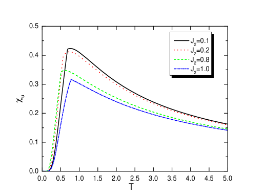
Figure 7: Uniform magnetic susceptibility $\chi_{u}$ versus $T$ for various $J_{2}$ values shown in the figure. Inset: the maximum height of $\chi_{u}(T)$ as a function of $J_{2}$. It is obtained using $2\times 2$ CMFT.

In the end, we calculate magnetic susceptibilities as functions of temperature. The uniform susceptibility $\chi_{u}$ (shown in Fig.7) obeys Curie-Weiss law at high temperatures. For any value of $J_{2}$ that we studied, $\chi_{u}$ reaches zero exponentially in the $T=0$ limit, forming a peak at some finite temperature. The disappearance of $\chi_{u}$ at $T=0$ shows that there is a finite gap in the magnetic excitation. This may be an artefact due to the small cluster that we used as well as due to the mean-field approximation. At the transition temperature, a cusp in $\chi_{u}(T)$ is observed, reflecting the singularity at the phase transition. In Fig. 8, N$\acute{e}$el staggered susceptibility $\chi_{n}$ and collinear staggered susceptibility $\chi_{c}$ are shown for $J_{2}=0.2$ and $0.8$. The divergences in $\chi_{n}(T)$ for $J_{2}=0.2$ and in $\chi_{c}(T)$ for $J_{2}=0.8$ are consistent with the finite temperature transition, while $\chi_{n}(T)$ for $J_{2}=0.8$ and $\chi_{c}(T)$ for $J_{2}=0.2$ only show a cusp or kink at the transition temperatures.

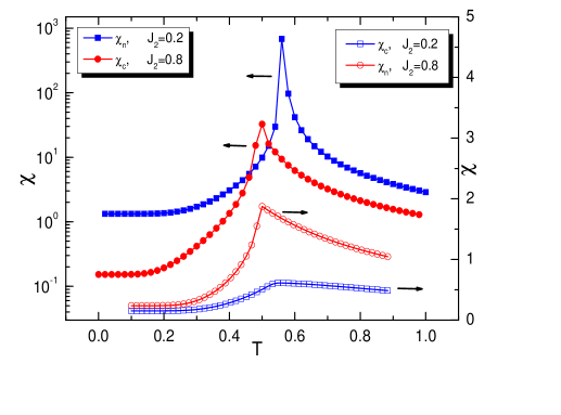
Figure 8: The solid squares and dots with eye-guiding lines are $\chi_{n}$ at $J_{2}=0.2$ and $\chi_{c}$ at $J_{2}=0.8$, respectively. They show divergence at the transition temperature. The empty squares and dots with eye-guiding lines are $\chi_{c}$ at $J_{2}=0.2$ and $\chi_{n}$ at $J_{2}=0.8$, respectively.

4 Summary

In summary, we use the cluster mean-field theory to study the $J_{1}$-$J_{2}$ Heisenberg model on a square lattice. For small, intermediate, and large $J_{2}/J_{1}$ regime, we obtain the N$\acute{e}$el AFM phase, the non-magnetic phase, and the collinear AFM phase, respectively. The N$\acute{e}$el-to-non-magnetic transition is found to be of second order, and the non-magnetic-to-collinear transition is of first order. The respective critical values $J_{2}^{c1}$ and $J_{2}^{c2}$ are found to converge rapidly with increasing $L$. From the largest $4\times 4$ cluster we obtain obtain $J_{2}^{c1}\approx 0.42$, which is very close to the results of $2\times 2$ cluster $0.41$. Extrapolating the cluster size to infinity, we obtain $J_{2}^{c2}\approx 0.59$. Both $J_{2}^{c1}$ and $J_{2}^{c2}$ agree with the previous results very well. We also investigate the finite temperature phase diagram, which due to the mean-field approximations, resembles that of the anisotropic $J_{1}-J_{2}$ model. The first order transition in $J_{2}>J_{2}^{c2}$ regime changes into a second order transition at $T>T_{c}$. Various susceptibilities are discussed to help us understand the system’s behavior near critical point. Our results show that the cluster mean-field theory is not only a very useful tool for studying classical phase transitions[49], but can also give surprisingly accurate ground state phase boundaries for the frustrated quantum magnet.

5 Acknowledgement

This work is supported by National Program on Key Basic Research Project (973 Program) under Grant No. 2009CB29100, 2012CB821402, and 2012CB921704, and by the NSFC under Grant No. 91221302 and 11074302.

References

References

- [1] P. W. Anderson, Scinence 235, 1196 (1987).
- [2] P. A. Lee, N. Nagaosa and X. G. Wen , Phys. Mod. Phys 78, 17 (2006).
- [3] P. Chandra and B. Doucot, Phys. Rev. B 38, 9335 (1988).
- [4] R. Melzi et al., Phys. Rev. Lett. 85, 1318 (2000); R. Melzi et al., Phys. Rev. B 64, 024409 (2001); G. Misguich, B. Bernu, and L. Pierre, Phys. Rev. B 68, 113409 (2003).
- [5] T. Yildirim, Phys. Rev. Lett. 101, 057010 (2008); F. Ma, Z. Y. Lu, and T. Xiang, Phys. Rev. B 78, 224517 (2008).
- [6] E. Dagotto and A. Moreo, Phys. Rev. Lett. 63, 2148 (1989).
- [7] H. J. Schulz and T. A. L. Ziman, Europhys. Lett. 18, 355 (1992).
- [8] J. Richter and J. Schulenburg, Eur. Phys. J. B 73, 117 (2010).
- [9] L. Capriotti and S. Sorella, Phys. Rev. Lett. 84, 3173 (2000).
- [10] M. Mambrini et al., Phys. Rev. B 74, 144422 (2006).
- [11] M. P. Gelfand, R. R. P. Singh, and D. A. Huse, Phys. Rev. B 40, 10801 (1989).
- [12] M. P. Gelfand, Phys. Rev. B 42, 8206 (1990).
- [13] R. R. P. Singh, Z. Weihong, C. J. Hamer, and J. Oitmaa, Phys. Rev. B 60, 7278 (1999).
- [14] R. R. P. Singh et al., Phys. Rev. Lett. 91, 017201 (2003).
- [15] J. Sirker, Z. Weihong, O. P. Sushkov, and J. Oitmaa, Phys. Rev. B 73, 184420 (2006).
- [16] D. Schmalfuß et al., Phys. Rev. Lett. 97, 157201 (2006).
- [17] R. Darradi et al., Phys. Rev. B 78, 214415 (2008).
- [18] A. V. Dotsenko and O. P. Sushkov, Phys. Rev. B 50, 13821 (1994).
- [19] L. Siurakshina, D. Ihle, and R. Hayn, Phys. Rev. B 64, 104406 (2001).
- [20] H. C. Jiang, H. Yao and L. Balents, Phys. Rev. B 86, 094417 (2012).
- [21] V. Murg, F. Verstraete, and J. I. Cirac, Phys. Rev. B 79, 195119 (2009).
- [22] J. F. Yu and Y. J. Kao, Phys. Rev. B 85, 094407(2012).
- [23] S. furukawa, M. sato, S. Onoda, and A. Furusaki, Phys. Rev. B 86, 094417 (2012).
- [24] L. Wang, Z. C. Gu, F. Verstraete, and X. G. Wen, arXiv:1112.3331.
- [25] G. Misguich, B. Bernu, and L. Pierre, Phys. Rev. B 68, 113409 (2003).
- [26] L. Capriotti, F. Becca, A. Parola, and S. Sorella, Phys. Rev. Lett. 87, 097201 (2001)
- [27] T. Li, F. Becca, W. Hu, and S. Sorella, Phys. Rev. B 86, 075111 (2012).
- [28] K. S. D. Beach, Phys. Rev. B 79, 224431 (2009).
- [29] W. J. Hu, F. Becca, A. Parola, and S. Sorella, arXiv:1304.2630.
- [30] Z. Cai, S. Chen, S. Kou, and Y. Wang, Phys. Rev. B 76, 054443 (2007).
- [31] M. E. Zhitomirsky and K. Ueda, Phys. Rev. B 54,9007 (1996).
- [32] H. T. Ueda and K. Totsuka, Phys. Rev. B 76, 214428 (2007).
- [33] F. Mila, D. Poilblanc, and C. Bruder, Phys. Rev. B 43, 7891 (1991).
- [34] L. Isaev, G. Ortiz, and J. Dukelsky, Phys. Rev. B 79, 024409 (2009).
- [35] P. Chandra, P. Coleman, and A. I. Larkin, Phys. Rev. Lett. 64, 88 (1990).
- [36] K. Takano, Y. Kito, Y. Ono, and K. Sano, Phys. Rev. Lett. 91, 197202 (2003).
- [37] V. Lante and A. Parola, Phys. Rev. B 73, 094427 (2006).
- [38] M. Mambrini, A. Luchli, D. Poilblanc and F. Mila, Phys. Rev. B 74, 14442 (2006).
- [39] A. W. Sandvik, Phys. Rev. B 85, 134407 (2012).
- [40] T. Senthil et al. Science 303, 1490 (2004).
- [41] J. H. Dai, Q. Si, J. X. Zhu and E. Abrahams, Proc. Natl Acad. Sci. USA 106, 4118 (2009).
- [42] E. M. Bruning et al. Phys. Rev. Lett. 101, 117206 (2008).
- [43] N. D. Mermin and H. Wagner, Phys. Rev. Lett. 17, 1133 (1966).
- [44] C. Weber et al., Phys. Rev. Lett. 91, 177202 (2003).
- [45] L. Capriotti, A. Fubini, T. Roscilde, and V. Tognetti, Phys. Rev. Lett. 92, 157202 (2004).
- [46] J. R. Viana and J. R. de Sousa, Phys. Rev. B 75, 052403 (2007).
- [47] H. Y. Wang, Phys. Rev. B 86, 144411 (2012).
- [48] P. Weiss, J. Phys. Radium 6, 661 (1907).
- [49] For a recent development, see D. Yamamoto, Phys. Rev. B 79, 144427 (2009).
- [50] N. H. Tong and F. C. Pu, Phys. Rev. B 62, 9425 (2000); ibid. 64, 235109 (2001); 70, 085118 (2004).
- [51] A. W. Sandvik, Phys. Rev. B 56, 11678 (1997); M. Calandra Buonaura and S. Sorella, Phys. Rev. B 57, 11446 (1998).
- [52] H. A. Bethe, Proc. R. Soc. London, ser. A 150, 552 (1953).
- [53] R. E. Peierls, Proc. Cambridge Philos Soc. 32, 477 (1936).
- [54] P. R. Weiss, Phys. Rev. 74, 1493 (1948).
- [55] T. Oguchi, Prog. Theor. Phys. 13, 148 (1955).
- [56] J. B. Fouet, M. Mambrini, P. Sindzingre, and C. Lhuillier, Phys. Rev. B 67, 054411 (2003).