Gradient type optimization methods for electronic structure calculations

Abstract

The density functional theory (DFT) in electronic structure calculations can be formulated as either a nonlinear eigenvalue or direct minimization problem. The most widely used approach for solving the former is the so-called self-consistent field (SCF) iteration. A common observation is that the convergence of SCF is not clear theoretically while approaches with convergence guarantee for solving the latter are often not competitive to SCF numerically. In this paper, we study gradient type methods for solving the direct minimization problem by constructing new iterations along the gradient on the Stiefel manifold. Global convergence (i.e., convergence to a stationary point from any initial solution) as well as local convergence rate follows from the standard theory for optimization on manifold directly. A major computational advantage is that the computation of linear eigenvalue problems is no longer needed. The main costs of our approaches arise from the assembling of the total energy functional and its gradient and the projection onto the manifold. These tasks are cheaper than eigenvalue computation and they are often more suitable for parallelization as long as the evaluation of the total energy functional and its gradient is efficient. Numerical results show that they can outperform SCF consistently on many practically large systems.

1 Introduction

Electronic structure calculations have been widely used in chemistry, materials science, drug design and nano-science over the past decades because of its great advantage in predicting phase transformation in various materials and a few other useful properties, such as optics, electric conductivity and magnetics [28]. The computational complexity of simulations using the many-body Schrödinger equation is extremely expensive. One of the most fundamental advances is the Density Functional Theory (DFT) models. These models can be divided into two classes: Orbital Free DFT (OFDFT) model and Kohn-Sham DFT (KSDFT) model [24, 28, 39, 50]. Both of them can be formulated as either nonlinear eigenvalue or direct minimization problems under orthogonality constraints of wave functions, where the former corresponds to the first-order necessary optimality condition of the latter.

There are several approaches for discretizing the DFT models. The plane wave basis has been popular due to its advantage in expressing the kinetic energy term and the Hartree potential in simple forms. It has been used in a few softwares, such as ABINIT [1] and VASP [48]. However, this type of basis is often suitable for periodic systems which does not contain the realistic cases like vacancy and dislocation, and it is usually not suitable for isolated systems, such as molecules and clusters. Since the plane wave basis is globally defined in real space, it may not be efficient for massively parallel computing [30, 41]. The second type of approach is the so-called atom-centered basis set. Since a few number of basis can provide satisfying results, it has been applied in some other softwares, such as Gaussian [17] and SIESTA [42]. On the other hand, it is not easy to construct a practically complete basis [27]. Another popular discretization is the real space approaches, including the finite difference, finite element, finite volume, and wavelet methods [10, 11, 12, 13, 14, 18, 20, 30, 32, 44, 46, 56, 58]. They can handle computational domains with complicate geometries and diversified boundary conditions. In particular, the whole domain can be divided into low and high resolution parts according to the frequency of the wave functions. A complete basis sets can always be chosen. Although their degrees of freedom are large, the adaptive methods and multilevel methods [28] can be applied to reduce the computational complexity.

The most widely used method for solving the nonlinear eigenvalue formulation is the so-called self-consistent field (SCF) iteration. Despite its popularity there are two well known challenges in SCF. First, its computational cost is dominated by the eigenvalue computation. For a system with $N$ electrons, the $N$ smallest eigenvalues and their associated eigenvectors of the Hamiltonian must be computed at each iteration. Second, the convergence of SCF is not guaranteed either theoretically or numerically. Its performance is often unpredictable for large scale systems with small band gaps, even with the assistance of the charge density or potential mixing techniques [23, 38]. On the other hand, optimization methods for direct minimization problems have been proposed for electronic structure calculations [6, 26, 29, 33, 36, 39, 47]. Trust region methods [15, 16, 43] substitute the linear eigenvalue problem in SCF by the so-called trust-region subproblems, in which the objective function are local quadratic approximations to the total energy functional. Monotonic reduction of the total energy can be achieved under a suitable update of the trust-region radius. A direct constrained minimization (DCM) algorithm is designed in [54], where the new search direction is built from a subspace spanned by the current approximation to the optimal wave function, the preconditioned gradient and the previous search direction. Although many of these optimization based methods often have better theoretical convergence properties than SCF, a common observation is that they are not competitive to SCF when the latter works and they may converge slowly on large scale systems [25].

In this paper, we study gradient type optimization methods derived from the direct minimization formulation to solve both OFDFT and KSDFT models. Essentially, our approaches construct new trial points along the gradient on the Stiefel manifold, i.e., a manifold consisted of orthogonal matrices. The orthogonality is preserved by an operation called retraction [2] on the Stiefel manifold. Consequently, all theoretical properties of optimization on manifold [2] can be applied to our approaches naturally. A major computational advantage is that eigenvalue computation is no longer needed. The main costs of our approaches arise from the assembling of the total energy functional and its gradient on manifold and the execution of retractions. These tasks are cheaper than eigenvalue computation and they are often more suitable for parallelization. The numerical performance of our gradient methods is further improved by the state-of-the-art acceleration techniques such as Barzilai-Borwein steps and non-monotone line search with global convergence guarantees. Our approaches can quickly reach the vicinity of an optimal solution and produce a moderately accurate approximation, at least in our numerical examples.

Our main contribution is the demonstration that the simple gradient type methods can outperform SCF consistently on many practically meaningful systems based on real space discretization. Two types of retractions on Stiefel manifold are investigated. One preserves orthogonality by using a Crank-Nicolson-like scheme proposed in [52] for minimizing a general differentiable function on Stiefel manifold. The other adopts the QR factorization for orthogonalization explicitly with respect to a gradient step on the Stiefel manifold. Due to the orthogonality, every intermediate point along the gradient direction of the Stiefel manifold has full rank which ensures the stability when the Cholesky factorization is used to compute the QR factorization. To the best of the authors’ knowledge, it is the first time that the QR-based method is systematically studied for electronic structure calculations. Our methods are implemented within the software packages Octopus [31] for KSDFT and RealSPACES (developed by the State Key Laboratory of Scientific and Engineering Computing of the Chinese Academy of Sciences) for OFDFT, respectively. Numerical experiments show that they can be more efficient and robust than SCF on many instances. High parallel scalability can also be achieved. However, we should point out that their efficiency still depends on an efficient evaluation of the total energy functional and their gradients. Although the regularized SCF method in [51] can converge faster by using the Hessian of the total energy functional, it requires the gradient methods to compute the search direction from some quadratic or cubic subproblems.

The rest of the paper is organized as follows. In Section 2, we present the mathematical models of DFT models, their associated discretization and the SCF iteration algorithm. Our gradient type algorithms are described in Section 3. Numerical results are reported in Section 4 to illustrate the efficiency of our algorithms. Finally, some concluding remarks are given in Section 5.

2 Preliminaries

2.1 The KSDFT model

The KSDFT model was developed based on the theories established by Hohenberg, Kohn and Sham [24]. The essence of KSDFT is treating the many-body system as an equivalent system with non-interacting electrons in an effective mean field governed by the charge density [30]. Using this representation, KSDFT can describe the ground state exactly in principle using single-electron wave functions.

For a system with $M$ nuclei and $N$ electrons, let $r$ represent the spatial coordinate in three dimensions. The charge density under the KSDFT model is expressed as $\rho(r)=\sum_{i=1}^{N}|\phi_{i}(r)|^{2},$ where $\phi_{i}(r)$ is the $i$-th wave function associated with the non-interactive auxiliary system under the orthogonality constraint $\int_{\mathbb{R}^{3}}\phi_{i}(r)\phi_{j}(r)\mathrm{d}r=\delta_{ij},$ where $\delta_{ij}$ is the Dirac delta function. The kinetic energy of the system can be expressed by the $N$ independent orthonormalized wave functions

$$T_{KS}=\frac{1}{2}\sum_{i=1}^{N}\int_{\mathbb{R}^{3}}|\nabla\phi_{i}(r)|^{2}\mathrm{d}r.$$

The Hartree energy is written as

$$E_{H}(\rho)=\frac{1}{2}\int_{\mathbb{R}^{3}}V_{H}(\rho)\rho(r)\mathrm{d}r,$$

where $V_{H}(\rho)=\displaystyle\int_{\mathbb{R}^{3}}\frac{\rho(r^{\prime})}{|r-r^{\prime}|}\mathrm{d}r^{\prime}$ is the classical electrostatic average interaction between electrons. The exchange-correlation energy is defined as

$$E_{xc}(\rho)=\int_{\mathbb{R}^{3}}\varepsilon_{xc}(\rho)\rho(r)\mathrm{d}r,$$

where $\varepsilon_{xc}(\rho)$ is the exchange-correlation functional used to describe the quantum interaction between electrons [54]. Let $V_{ext}(r)$ be the external potential, the associated external potential energy is

$$E_{ext}=\int_{\mathbb{R}^{3}}V_{ext}(r)\rho(r)\mathrm{d}r.$$

Therefore, the total energy of the system is

(2.1) $$E_{KS}(\{\phi_{i}\})=T_{KS}+E_{H}+E_{xc}+E_{ext}+E_{II},$$

where $E_{II}=\displaystyle\frac{1}{2}\sum_{i,j=1,i\neq j}^{M}\frac{Z_{i}Z_{j}}{|R_{i}-R_{j}|}$ is the nuclei interaction energy and $Z_{i}$ and $R_{i}$ are the atomic number and coordinate of the $i$-th nucleus, respectively. For more details we refer the reader to [28]. Then finding the ground state energy of the system is equivalent to solving the following minimization problem:

(2.2) $$E_{KS}^{0}=\inf_{\phi_{i}\in H^{1}(\mathbb{R}^{3})} \quad E_{KS}(\{\phi_{i}\})$$

s.t. $$\int_{\mathbb{R}^{3}}\phi_{i}(r)\phi_{j}(r)\mathrm{d}r=\delta_{ij},\quad 1\leqslant i,j\leqslant N.$$

Alternatively, one solves the so-called KS equation

(2.3) $$\begin{cases}\mathcal{H}_{KS}\phi_{i}\triangleq\left(-\displaystyle\frac{1}{2}\Delta+V_{ext}(r)+V_{H}(\rho)+V_{xc}(\rho)\right)\phi_{i}=\displaystyle\sum_{j=1}^{N}\lambda_{ij}\phi_{j},\\ \displaystyle\int_{\mathbb{R}^{3}}\phi_{i}(r)\phi_{j}(r)\mathrm{d}r=\delta_{ij},\end{cases}$$

where $\displaystyle V_{xc}(\rho)=\frac{\delta E_{xc}(\rho)}{\delta\rho}$, $i,j=1,2,\cdots,N$. The KS equation (2.3) actually corresponds to the first-order necessary optimality condition of (2.2). It is a nonlinear eigenvalue problem since the Hamiltonian operator $\mathcal{H}_{KS}$ is a nonlinear operator with respect to the charge density $\rho$.

Although the KSDFT model has been very successful in many aspects, there still exists a few difficulties. First, it can be computationally demanding because of the determination of the $N$ wave functions whose cost is dominant. Second, the wave functions usually oscillate rapidly near the nuclei in realistic systems. Consequently, pseudopotential algorithm is always introduced. Third, approximations are needed for the unknown analytic formula of $V_{xc}(\rho)$ [34, 35].

2.2 The OFDFT model

The OFDFT model adopts the kinetic energy density functional (KEDF) as the kinetic energy term instead of the one in KSDFT. Hence, $N$ independent single-electron wave functions are no longer needed in OFDFT. One of the most successful orbital-free models is the so-called Thomas-Fermi-von Weizasäcker (TFW) model, whose kinetic energy has the following representation

(2.4) $$T_{TFW}(\rho)=C_{TF}T_{TF}(\rho)+\mu T_{vW}(\rho),$$

where $C_{TF}=\displaystyle\frac{3}{10}(3\pi^{2})^{\frac{2}{3}}$, $T_{TF}(\rho)=\displaystyle\int_{\mathbb{R}^{3}}\rho^{\frac{5}{3}}(r)\mathrm{d}r$, $T_{vW}(\rho)=\displaystyle\frac{1}{8}\int_{\mathbb{R}^{3}}\frac{|\nabla\rho|^{2}}{\rho}\mathrm{d}r$ and $\mu$ is the parameter that obtained based on physical experiments or theoretical analysis. Since TFW model considers the gradient of the charge density, it can deal with heterogeneous systems, especially for diatomic systems. A few other KEDFs were proposed in [49, 50] and references therein in order to satisfy the linear response theory. They share a common formula

(2.5) $$T_{LR}(\rho)=T_{TF}(\rho)+\mu T_{vW}(\rho)+C_{TF}\int_{\mathbb{R}^{3}}\int_{\mathbb{R}^{3}}K(r-r^{\prime})\rho^{\alpha}(r)\rho^{\beta}(r^{\prime})\mathrm{d}r\mathrm{d}r^{\prime},$$

where $K(r-r^{\prime})$ is chosen such that $T_{LR}(\rho)$ satisfies the Lindhard susceptibility function but using different parameters $\alpha$ and $\beta$. By abuse of notation, we use $T_{OF}(\rho)$ to denote either $T_{TFW}(\rho)$ or $T_{LR}(\rho)$. Subsequently, the total energy can be written as

(2.6) $$E_{OF}(\rho)=T_{OF}(\rho)+E_{ext}(\rho)+E_{H}(\rho)+E_{xc}(\rho)+E_{II},$$

where $E_{ext}(\rho)$, $E_{H}(\rho)$, $E_{xc}(\rho)$ and $E_{II}$ are defined the same as in (2.1). Since the charge density $\rho$ should be properly normalized to the number of electrons $N$ in the system, finding the ground state energy of the system can be formulated as

(2.7) $$E_{OF}^{0}=\inf\left\{E_{OF}(\rho):\rho\in L^{1}(\mathbb{R}^{3}),\ \rho^{\frac{1}{2}}\in H^{1}(\mathbb{R}^{3}),\ \rho\geq 0,\ \int_{\mathbb{R}^{3}}\rho(r)\mathrm{d}r=N\right\}.$$

The nonnegative constraints can be eliminated by substituting $\rho$ by another variable $\varphi^{2}$. The first-order necessary optimality condition of (2.7) with respect to KEDF (2.4) is the nonlinear eigenvalue problem

(2.8) $$\begin{cases}\mathcal{H}_{OF}\varphi\triangleq\left(-\displaystyle\frac{\mu}{2}\Delta+\displaystyle\frac{\delta\Big{(}T_{OF}(\rho)-\mu T_{vW}(\rho)\Big{)}}{\delta\rho}+V_{eff}(\rho)\right)\varphi=\lambda\varphi,\\ \displaystyle\int_{\mathbb{R}^{3}}\varphi^{2}=N,\end{cases}$$

where $\displaystyle\frac{\delta T_{vW}(\rho)}{\delta\rho}=-\frac{1}{2}\frac{\nabla^{2}\varphi}{\varphi}$ and $V_{eff}(\rho)=V_{ext}(r)+V_{H}(\rho)+V_{xc}(\rho)$.

Therefore, OFDFT model expresses the system by only using the charge density as its variable in the spirit of Hohenberg-Kohn theorem and avoids computing $N$ eigenpairs [8]. Numerical experiments have shown that OFDFT is good at simulating systems with main group elements and nearly-free-electron-like metals with comparable accuracy to KSDFT [21, 50]. However, the accuracy of OFDFT relies on the accuracy of KEDFs and the results may not be accurate for covalently bonded and ionic systems [21].

2.3 The discretized DFT models

In this subsection, we describe the real space discretization for KSDFT and OFDFT, respectively. Since going into the detailed discretizing steps would take us too far afield, we focus on a high level description without loss of generality. The readers are referred to [10, 12, 11, 58] for theoretical analysis of these discretization schemes.

Under a chosen finite difference discretization scheme, the $N$ independent wave functions can be represented by a matrix

$$X=[x_{1},\cdots,x_{N}]\in\mathbb{R}^{n\times N},$$

where $n$ is the spatial degrees of freedom of the computational domain $\Omega$, $\{x_{i}\}$ are column vectors used to approximate the wave functions $\{\phi_{i}\}$ and they satisfy the orthogonality constraint

$$X^{\top}X=I_{N},$$

where $I_{N}$ is the $N\times N$ identity matrix. The discretized charge density associated with these $N$ occupied states can be expressed as

$$\rho(X)=\mathrm{diag}(XX^{\top}),$$

where $\mathrm{diag}(A)$ is a column vector consisting of diagonal entries of the matrix $A$. Hence, the discretized total energy functional of (2.1) is

(2.9) $$E_{KS}(X)=\frac{1}{2}\mathrm{tr}(X^{\top}LX)+\mathrm{tr}(X^{\top}EX)+\frac{1}{2}\rho(X)^{\top}L^{{\dagger}}\rho(X)+\rho(X)^{\top}\epsilon_{xc}(\rho(X)),$$

where the Hermitian matrix $L\in\mathbb{R}^{n\times n}$ is an approximation to the Laplacian operator, the diagonal matrix $E$ is an approximation of $V_{ext}$, and the discretized form of the Hartree potential can be represented by the product of Hermitian matrix $L^{\dagger}$ with $\rho(X)$, where $L^{\dagger}$ is the inverse of the discretized Laplacian operator.

Therefore, the discretized minimization problem (2.2) is

(2.10) $$\min_{X\in\mathbb{R}^{n\times N}}E_{KS}(X),\ \quad\mbox{s.t.}\ \ X^{\top}X=I_{N}.$$

Using the notation $((E_{KS})_{X})_{i,j}=\frac{\partial E_{KS}}{\partial X_{ij}}$ for the partial derivative, we obtain

(2.11) $$(E_{KS})_{X}=H(X)X,$$

where $H(X)$ is the discretized Hamiltonian matrix

(2.12) $$H(X)=\frac{1}{2}L+E+\mathrm{Diag}(L^{\dagger}\rho(X))+\mathrm{Diag}(\gamma_{xc}),$$

where $\mathrm{Diag}(v)$ denotes a diagonal matrix with $v$ on its diagonal, and

$$\gamma_{xc}(\rho)=\frac{\mathrm{d}[\rho\epsilon_{xc}(\rho)]}{\mathrm{d}\rho}.$$

Consequently, the first-order necessary optimality condition of problem (2.10) is

(2.13) $$H(X)X =X\Lambda,$$

$$X^{\top}X =I_{N},$$

where $\Lambda$ is the Lagrangian multiplier which is a symmetric matrix. Hence, (2.13) is exactly the discretization of the continuous KS equation (2.3).

We choose the finite element method to discretize the OFDFT model. Assume that the finite element basis sets under a shape-regular tetrahedral conforming mesh of $\Omega$ are $\{u_{k}\}^{n}_{k=1}$, where $n$ is the number of the basis functions. The wave function $\varphi$ can be approximated by a linear combination of these finite element basis

(2.14) $$\varphi(c)=\sum^{n}_{t=1}c_{t}u_{t},$$

where $c=(c_{1},c_{2},\cdots,c_{n})^{\top}$. The corresponding discretized charge density can be expressed as

$$\rho(c)=\varphi^{2}(c).$$

The discretization of the nonlinear eigenvalue problem (2.8) is

(2.15) $$\int_{\Omega}u_{k}\mathcal{H}_{OF}\varphi(c)\mathrm{d}r=\lambda\int_{\Omega}u_{k}\varphi(c)\mathrm{d}r,\ \ 1\leq k\leq n,$$

Substituting (2.14) into (2.15) and running over all the indices, we obtain the following generalized eigenvalue problem

(2.16) $$H(c)c=\lambda Bc,$$

where the components of $H(c)$ and $B$ are

$$H_{kl}(c)=\int_{\Omega}u_{k}\mathcal{H}_{OF}u_{l}\mathrm{d}r,\quad\mathrm{and}\quad B_{kl}=\int_{\Omega}u_{k}u_{l}\mathrm{d}r.$$

The corresponding discretization of (2.7) is

(2.17) $$\min_{c\in\mathbb{R}^{n}}E_{OF}(\rho(c)),\quad\mbox{s.t.}\ \ c^{\top}Bc=1.$$

2.4 The self-consistent field (SCF) iteration

The nonlinear eigenvalue formulations of KSDFT and OFDFT presented in subsection 2.3 give rise to the SCF iteration naturally. Without loss of generality, we describe the SCF iteration for the discretized KS equation (2.13). Starting from $X_{0}$ with $X_{0}^{\top}X_{0}=I$, the basic SCF iteration computes the $(k+1)$-th iterate $X_{k+1}$ as the solution of the linear eigenvalue problem:

(2.18) $$H(X_{k})X_{k+1} =X_{k+1}\Lambda_{k+1},$$

$$X_{k+1}^{\top}X_{k+1} =I.$$

The convergence of the SCF iteration can often be speeded up by the so-called charge density or potential mixing techniques. The only difference is that the coefficient matrix $H(X_{k})$ in the linear eigenvalue problem (2.18) is replaced by another matrix $H$, which is constructed from a linear combination of the previously computed charge densities or potentials and the one obtained from certain schemes at current iteration. Frequently used schemes include Anderson’s mixing [3], Pulay’s mixing (or DIIS) [38] and Broyden mixing [23]. We outline the major steps of the SCF iteration in Algorithm 1.

1 Given an initial guess on the charge density $\rho^{0}_{in}$.

2

3Solve the linear eigenvalue problem

$$H(\rho_{in}^{k})X_{k+1}=X_{k+1}\Lambda_{k+1},\quad X_{k+1}^{\top}X_{k+1}=I_{N},$$

where $H(\rho_{in}^{k})$ is the Hamiltonian at $\rho_{in}^{k}$, $X_{k+1}$ are the eigenvectors corresponding to the $N$-smallest eigenvalues of $H(\rho_{in}^{k})$.

4

5Compute the new charge density $\rho_{out}^{k+1}$ from $X_{k+1}$. Stop if a certain termination rule is met.

Compute a new charge density $\rho_{in}^{k+1}$ using $\rho_{out}^{k+1}$ and a prior chosen density mixing scheme and go to step 2.

Algorithm 1 The SCF Iteration

Although the SCF iteration with charge density or potential mixing often works well on many problems, it is well known that there is no theoretical guarantee on its convergence and it can converge slowly or even fail on certain problems [54] . On the other hand, the main computational bottleneck of the SCF iteration is solving a sequence of linear eigenvalue problems. Since the degrees of freedom $n$ is usually very large, in particular for large-scale systems, the computational cost of eigenpairs is the dominant factor of the SCF iteration.

3 Gradient type algorithms for total energy minimization

The minimization models (2.2) and (2.7) provide many alternative methodologies other than solving linear eigenvalue problems repeatedly. Since $B$ in (2.17) is positive definite, (2.17) can be transformed to a minimization problem under a unit spherical constraint as

(3.19) $$\min_{y\in\mathbb{R}^{n}}E_{OF}(\rho(B^{-\frac{1}{2}}y)),\ \ \mbox{s.t.}\ \ \|y\|_{2}=1.$$

Therefore, both the KSDFT model (2.10) and the OFDFT model (3.19) are unified under optimization with orthogonality constraints as

(3.20) $$\min_{X\in\mathbb{R}^{n\times p}}E(X),\ \ \mbox{s.t.}\ \ X^{\top}X=I_{p},$$

where $E(X)$ is the corresponding total energy functional of either KSDFT or OFDFT models and $p$ is the number of eigenpairs needed to be calculated. Inspired by the preliminary but promising performance of the feasible method for (3.20) in [52], we further investigate gradient type methods for solving OFDFT and KSDFT, including one approach using QR factorization [2]. Each trial point generated by these methods is guaranteed to be on the unit sphere or satisfy the orthogonality constraints. These schemes are numerically efficient and let us apply state-of-the-art acceleration techniques such as Barzilai-Borwein steps and non-monotone line search with global convergence guarantees.

Let $\mathcal{M}_{n}^{p}=\{X\in\mathbb{R}^{n\times p}:X^{\top}X=I\}$ be the feasible set, which is often referred to the Stiefel manifold. When $p=1$, it reduces to the unit-sphere manifold $S^{n-1}=\{x\in\mathbb{R}^{n}:\|x\|_{2}=1\}$. The tangent space of $\mathcal{M}_{n}^{p}$ at $X$ is

$$\mathcal{T}_{X}\mathcal{M}_{n}^{p}=\{Z\in\mathbb{R}^{n\times p}:X^{\top}Z+Z^{\top}X=0\}.$$

The gradient $\nabla E(X)$ at $X$ is defined as the element of $\mathcal{T}_{X}\mathcal{M}_{n}^{p}$ that satisfies

(3.21) $$\mathrm{tr}(E^{\top}_{X}\Delta)=\left\langle\nabla E,\Delta\right\rangle_{X}:=\mathrm{tr}\left(\nabla E^{\top}(I-\frac{1}{2}XX^{\top})\Delta\right),\quad\mbox{ for all }\Delta\in\mathcal{T}_{X}\mathcal{M}_{n}^{p},$$

where $E_{X}$ is the partial derivative of $E(X)$, i.e., $(E_{X})_{ij}=\Big{(}\mathcal{D}E(X)\Big{)}_{ij}=\displaystyle\frac{\partial E_{KS}}{\partial X_{ij}}$. For the KSDFT and OFDFT models, it holds

(3.22) $$E_{X}=H(X)X,$$

where $H(X)$ is the corresponding Hamiltonian matrix. An elementary verification shows that

(3.23) $$\nabla E(X)=E_{X}-XE_{X}^{\top}X.$$

The first-order optimality conditions of (3.20) are

$$\nabla E(X)=0,\mbox{ and }X^{\top}X=I.$$

Our proposed algorithms are adapted from the classical steepest descent method. The orthogonality constraints are preserved at a reasonable computational cost. Since $\nabla E$ is the gradient on the manifold, a natural idea is to compute the next iterates as

(3.24) $$Y=X-\tau\nabla E(X),$$

where $\tau$ is a step size. The obstacle is that the new point $Y$ may not satisfy $Y\in\mathcal{M}_{n}^{p}$. We next describe two approaches for overcoming this difficulty.

Our first strategy uses the constraint-preserving scheme proposed in [52] by slightly modifying the term $\nabla E(X)$. Suppose that $X^{\top}X=I$ and define $W$ as a skew-symmetric matrix

$$W:=E_{X}X^{\top}-XE_{X}^{\top},$$

which yields $\nabla E(X)=WX$. Then the new trial point is generated as

(3.25) $$X_{\mathrm{WY}}(\tau)=X-\tau W\left(\frac{X+X_{\mathrm{WY}}(\tau)}{2}\right).$$

It can be shown that $X_{\mathrm{WY}}(\tau)$ is a orthogonal matrix and it defines a projected gradient-like curve on the Stiefel manifold.

Lemma 3.1 (Lemmas 3 and 4 in [52]).

1) The matrix $X_{\mathrm{WY}}(\tau)$ defined by (3.25) can be expressed as

(3.26) $$X_{\mathrm{WY}}(\tau)=\left(I+\frac{\tau}{2}W\right)^{-1}\left(I-\frac{\tau}{2}W\right)X,$$

which satisfies $X_{\mathrm{WY}}(\tau)^{\top}X_{\mathrm{WY}}(\tau)=X^{\top}X$ and $X_{\mathrm{WY}}^{\prime}(0)=-\nabla E(X)$.

2) Rewrite $W=UV^{\top}$ for $U=[E_{X},\;X]$ and $V=[X,\;-E_{X}]$. If $I+\frac{\tau}{2}V^{\top}U$ is invertible, then (3.26) is equivalent to

(3.27) $$X_{\mathrm{WY}}(\tau)=X-\tau U\left(I+\frac{\tau}{2}V^{\top}U\right)^{-1}V^{\top}X.$$

3) Suppose $p=1$ and $W=ax^{\top}-xa^{\top}$, where $a=E_{x}$. Then (3.26) is given explicitly by

(3.28) $$x_{\mathrm{WY}}(\tau)=x-\beta_{1}(\tau)a-\beta_{2}(\tau)x,$$

where $\beta_{1}(\tau)=\tau\frac{x^{\top}x}{1-\left(\frac{\tau}{2}\right)^{2}(a^{\top}x)^{2}+\left(\frac{\tau}{2}\right)^{2}\|a\|^{2}_{2}\|x\|^{2}_{2}}$ and $\beta_{2}(\tau)=-\tau\frac{x^{\top}a+\frac{\tau}{2}\left((a^{\top}x)^{2}-(a^{\top}a)(x^{\top}x)\right)}{1-\left(\frac{\tau}{2}\right)^{2}(a^{\top}x)^{2}+\left(\frac{\tau}{2}\right)^{2}\|a\|^{2}_{2}\|x\|^{2}_{2}}$.

Using the convention that an $m\times p$ matrix times a $p\times n$ matrix costs $2mnp$ flops, we calculate the computational complexity of the scheme (3.25) as below. The cost of the scheme (3.25) reduces to two inner products in case of $p=1$. When $1<p\ll n$, the formula (3.27) should be used to compute $X_{\mathrm{WY}}(\tau)$ whose cost is $7np^{2}+\frac{40}{3}p^{3}+O(np)$. This number shows that the complexity depends on both the spatial degrees of freedom $n$ and the number of columns $p$. Although orthogonality is preserved theoretically, we observe in our numerical experiments that it may lose due to numerical errors and a reorthogonalization step is needed. Further analysis on controlling the errors can be found in [55].

Our second strategy is to orthogonalize $Y$ explicitly by using the QR factorization

(3.29) $$X_{\mathrm{QR}}(\tau)=\mathrm{qr}(Y),$$

where $\mathrm{qr}(Y)$ is the column-orthogonal matrix $Q$ corresponding to the QR factorization of $Y=QR$. Therefore, the update scheme (3.29) can be viewed as a kind of projected gradient method on the Stiefel manifold. The next proposition shows that the matrix $Y$ in (3.24) is always full rank and the condition number of matrix $Y^{\top}Y$ is bounded if the step size $\tau$ and the norm of $\|H(X)\|_{2}$ are bounded.

Proposition 3.1.

Suppose that $X\in\mathbb{R}^{n\times p}$ satisfies $X^{\top}X=I$. Then the matrix $Y$ computed by (3.24) is full rank for any $\tau\in\mathbb{R}$ and the eigenvalue of $Y^{\top}Y$ is bounded as

(3.30) $$1\leqslant\lambda(Y^{\top}Y)\leqslant\tau^{2}\|H(X)\|_{2}^{2}+1.$$

Proof.

Since $Y=X-\tau\nabla E(X)$, we have

$$Y^{\top}Y =X^{\top}X-\tau(\nabla E(X)^{\top}X+X^{\top}\nabla E(X))+\tau^{2}\nabla E(X)^{\top}\nabla E(X).$$

The definition of $\nabla E(X)$ in (3.23) and $X^{\top}X=I$ yield

$$\nabla E(X)^{\top}X+X^{\top}\nabla E(X) =(E_{X}^{\top}-X^{\top}E_{X}X^{\top})X+X^{\top}(E_{X}-XE_{X}^{\top}X),$$

$$=E_{X}^{\top}X-X^{\top}E_{X}+X^{\top}E_{X}-E_{X}^{\top}X=0,$$

which further gives

$$Y^{\top}Y=I+\tau^{2}\nabla E(X)^{\top}\nabla E(X).$$

Since $\nabla E(X)^{\top}\nabla E(X)$ is positive semidefinite and its largest eigenvalue is $\|\nabla E(X)\|^{2}_{2}$, we obtain

(3.31) $$1\leqslant\lambda(Y^{\top}Y)\leqslant\tau^{2}\|\nabla E(X)\|_{2}^{2}+1.$$

Substituting the expression of $E_{X}$ in (3.22) into $\nabla E(X)$ and using the fact $I-XX^{\top}$ is a projection, we have

(3.32) $$\|\nabla E(X)\|_{2}\leqslant\|(I-XX^{\top})H(X)X)\|_{2}\leq\|H(X)\|_{2}.$$

Combining (3.31) and (3.32) together proves (3.30). ∎

There are many approaches for computing the QR factorization. Propositon 3.1 implies that the matrix $Y^{\top}Y$ is well-conditioned under a suitable chosen step size $\tau$. Hence, the QR factorization based on the Cholesky factorization can be computed stably and accurately, for example, using the efficient implementation in LAPACK. Specifically, the matrix $Q$ can be assembled as in Algorithm 2.

1Input the matrix $Y$.

2 Compute the Cholesky factorization $LL^{\top}$ of $Y^{\top}Y$.

Output $Q=YL^{-1}$.

Algorithm 2 Cholesky QR factorization

Using the same notation as our analysis for the complexity of scheme (3.25), the cost of scheme (3.29) is $6np^{2}+\frac{1}{3}p^{3}+O(np)$ since computing the gradient $\nabla E(X)$ and the QR-factorization need $4np^{2}$ and $2np^{2}+\frac{1}{3}p^{3}+O(np)$, respectively. We can see that the QR-based method is slightly cheaper than the first strategy.

Another critial algorithmic issue is the determination of a suitable step size $\tau$. Instead of using the classical Armijo-Wolfe based monotone line search, we apply the nonmonotone curvilinear (as our search path is on the manifold rather than a straight line) search with an initial step size determined by the Barzilai-Borwein (BB) formula, which we have found more efficient for our problem. They were developed originally for the vector case in [4]. At iteration $k$, the step size is computed as

(3.33) $$\tau_{k,1}=\frac{\mathrm{tr}\left((S_{k-1})^{\top}S_{k-1}\right)}{|\mathrm{tr}\big{(}(S_{k-1})^{\top}Y_{k-1}\big{)}|}\quad\mbox{ or }\quad\tau_{k,2}=\frac{|\mathrm{tr}\left((S_{k-1})^{\top}Y_{k-1}\right)|}{\mathrm{tr}\big{(}(Y_{k-1})^{\top}Y_{k-1}\big{)}},$$

where $S_{k-1}=X_{k}-X_{k-1}$ and $Y_{k-1}=\nabla E(X_{k})-\nabla E(X_{k-1})$. In order to guarantee convergence, the final value for $\tau_{k}$ is a fraction (up to 1, inclusive) of $\tau_{k,1}$ or $\tau_{k,2}$ determined by a nonmonotone search condition. Let $X(\tau)$ be either of (3.25) or (3.29), $C_{0}=E(X_{0})$, $Q_{k+1}=\eta Q_{k}+1$ and $Q_{0}=1$. The new points are generated iteratively in the form $X_{k+1}:=X_{k}(\tau_{k})$, where $\tau_{k}=\tau_{k,1}\delta^{h}$ or $\tau_{k}=\tau_{k,2}\delta^{h}$ and $h$ is the smallest nonnegative integer satisfying

(3.34) $$E(X_{k}(\tau_{k}))\leq C_{k}-\rho_{1}\tau_{k}\|\nabla E(X_{k})\|_{F}^{2},$$

where each reference value $C_{k+1}$ is taken to be the convex combination of $C_{k}$ and $E(X_{k+1})$ as $C_{k+1}=(\eta Q_{k}C_{k}+E(X_{k+1}))/Q_{k+1}$. In Algorithm 3 below, we specify our method for solving the DFT models. Although several backtracking steps may be needed to update the $X_{k+1}$, we observe that the BB step size $\tau_{k,1}$ or $\tau_{k,2}$ is often sufficient for (3.34) to hold in most of our numerical experiments. In the case that $\tau_{k,1}$ or $\tau_{k,2}$ is not bounded, they are reset to a finite number and convergence of our algorithm still holds.

1Given $X_{0}$, set $\tau>0$, $\rho_{1},\delta,\eta,\epsilon\in(0,1)$, $k=0$.

2 while $\|\nabla E(X_{k})\|>\epsilon$  do

3       Compute $\tau_{k}\leftarrow\tau_{k,1}\delta^{h}$ or $\tau_{k}\leftarrow\tau_{k,2}\delta^{h}$, where $h$ is the smallest nonnegative integer satisfying the condition (3.34).

4       Set $X_{k+1}\leftarrow X_{\mathrm{QR}}(\tau)$ or $X_{k+1}\leftarrow X_{\mathrm{WY}}(\tau)$.

5       $Q_{k+1}\leftarrow\eta Q_{k}+1$ and $C_{k+1}\leftarrow(\eta Q_{k}C_{k}+E(X_{k+1}))/Q_{k+1}$.

6       $k\leftarrow k+1$.

Calculate the ground state energy and other physical quantities.

Algorithm 3 Constraint Optimization on Stiefel Manifold

We next summarize the computational complexity of Algorithm 3 with respect to schemes (3.25) and (3.29), respectively. Each iteration of (3.25) has a minimal complexity of $9np^{2}+\frac{40}{3}p^{3}+O(np)$ since the cost of computing $X_{WY}(\tau)$ is $7np^{2}+\frac{40}{3}p^{3}+O(np)$ and the assembling of the gradient $\nabla E(X)$ for the BB step size needs another $2np^{2}$. The work for a different $\tau$ is $4np^{2}+O(p^{3})$ because of the saving of some intermediate variables. On the other hand, the minimal cost of each iteration of the QR-based method (3.29) is $6np^{2}+\frac{1}{3}p^{3}+O(np)$. The cost for a different $\tau$ during backtracking line search is that of a new QR-factorization because $\nabla E(X)$ is available. When $p$ is larger than a few hundreds, the inversion of $I+\frac{\tau}{2}V^{\top}U$ in (3.27) is not negligible and the LU decomposition is usually more expensive than the Cholesky factorization.

We make the following assumption for the convergence of our gradient type methods.

Assumption 3.1.

The total energy function $E(X)$ is differentiable and its derivative $E_{X}(X)$ is Lipschitz continuous with Lipschitz constant $L_{0}$, i.e.,

$$\|E_{X}(X)-E_{X}(Y)\|_{F}\leq L_{0}\|X-Y\|_{F},\ \text{for all}\ X,\ Y\in\mathcal{M}^{p}_{n}.$$

Although Assumption 3.1 may not be satisfied in many cases due to the exchange-correlation term, it holds in cases such as the Gross-Pitaevskii equation [57]. Using the proofs of [55] in a similar fashion, we can establish the convergence of Algorithm 3 as follows.

Theorem 3.1.

Suppose that Assumption 3.1 holds. Let $\{X_{k}\mid k\geq 0\}$ be a sequence generated by Algorithm 3 using $\epsilon=0$, $\tau_{k}=\tau_{k,1}\delta^{h}$ and $\rho_{1}<\frac{1}{2}$. Then the step size satisfies

$$\tau_{k}\geq\min\{c,\tau_{k,1}\},$$

where $c$ is some constant. Furthermore, either $\|\nabla E(X_{k})\|=0$ for some finite $k$ or

$$\liminf_{k\rightarrow\infty}\|\nabla E(X_{k})\|_{F}=0.$$

We should point out that both schemes (3.25) and (3.29) are special cases of optimization on manifold in [2]. A map $\mathcal{R}:\mathcal{T}_{X}\mathcal{M}\to\mathcal{M}$ is called a retraction if

1. $\mathcal{R}(0_{X})=X$, where $0_{X}$ is the origin of $\mathcal{T}_{X}$.

2. ${\frac{\mathrm{d}}{\mathrm{d}t}}\mathcal{R}(tU)|_{t=0}=U$, for all $U\in\mathcal{T}_{X}$.

It can be verified that both schemes (3.25) and (3.29) are retractions. They map a tangent vector of $\mathcal{M}_{n}^{p}$ at $X$ to a member on $\mathcal{M}_{n}^{p}$. Global convergence of the algorithms using monotone line search schemes can be obtained under some mild conditions [2]. There are many other types of retractions. They can be applied to solve OFDFT and KSDFT as long as their computational cost is not expensive.

The discretization on a fine mesh for large-scale systems usually leads to a problem of huge size whose computational cost is expensive. A useful technique is adaptive mesh refinement, where the discretized problems are solved in turn from the coarsest mesh to the finest mesh and the starting point at each level other than the coarsest is obtained by projecting the solution obtained on the previous (i.e., next coarser) mesh. We present our adaptive mesh refinement method in Algorithm 4.

1

2Given an initial mesh $\mathcal{T}_{0}$ and initial wavefunctions $\hat{X}^{0}$. Set $i=1$.

3Use $\hat{X}^{i-1}$ as an initial guess on the $i$-th mesh $\mathcal{T}_{i}$ to calculate the ground state wavefunctions $\hat{X}^{i}$ using Algorithm 3.

4Calculate a posteriori error estimator $\eta_{i}$ on mesh $\mathcal{T}_{i}$. If $\eta_{i}<\epsilon$, evaluate physical quantities and stop. Otherwise, mark and refine the mesh to obtain $\mathcal{T}_{i+1}$, and go to step 4.

Algorithm 4 Adaptive Mesh Refinement Method on Stiefel Manifold

4 Numerical experiments

We now demonstrate the efficiency and robustness of our gradient type methods for solving both KSDFT and OFDFT models. All experiments are performed on a PC cluster LSSC-III in the State Key Laboratory of Scientific and Engineering Computing, Chinese Academy of Sciences. Each node of LSSC-III contains two Intel X5550 GPUs and 24GB memory. Our implementation is parallelized by using MPI. Throughout our numerical experiments, we use Troullier-Martins norm conserving pseudopotentials [45] and choose local density approximation (LDA) to approximate $V_{xc}(\rho)$ [24].

4.1 Numerical results for the KSDFT model

In this subsection, we compare the gradient type method using (3.25) (denoted by “OptM-WY”) and the one using (3.29) (denoted by “OptM-QR”) with the SCF iteration on KSDFT. The source code of SCF is taken from the software Octopus (version 4.0.1) [31], an open source ab initio real-space computing platform using finite difference discretization. Both gradient type methods are implemented based on Octopus and they use the same computational subroutines as SCF wherever it is possible. The reported total energy functional is computed according to (2.1) rather than the original one in Octopus based on precalculated eigenvalues. However, these two formulas are equivalent mathematically. The initial guess is generated by linear combination of atomic orbits (LCAO) method. All three methods are terminated if residuals of the gradient on manifold is smaller than some prescribed tolerance $\varepsilon_{g}$, that is,

$$\|E_{X}-XE_{X}^{T}X\|_{F}\leq\varepsilon_{g}.$$

For SCF, the Broyden method is used as the charge density mixing strategy. The linear eigenvalue problem is solved by a preconditioned conjugate gradient method (PCG) and it is terminated if the residual of the eigenpairs is smaller than $0.1\varepsilon_{g}$ or the number of iterations reaches 25. In fact, we have tested most eigensolvers available in Octopus, including PCG, a new CG method developed in [22], a preconditioned Lanczos Scheme [40], and LOBPCG. The reason of choosing PCG is that it is one of the best methods in our tests. Since the gradient type methods may stagnate when the iterates are close to the solution, especially for large scale systems, we also terminate if the relative change of the total energy functional is small, i.e., $\frac{df_{k}+df_{k-1}+df_{k-2}}{3}<10^{-13}$, where $df_{k}=\displaystyle\frac{|E(X_{k-1})-E(X_{k})|}{|E(X_{k-1})|+1}$ for the $k$-th iteration step. An orthogonalization step is executed in OptM-WY if $\|X^{\top}X-I\|_{F}>10^{-12}$ to enforce orthogonality.

We choose eight typical molecular systems, including benzene ($C_{6}H_{6}$), valine ($C_{5}H_{9}O_{2}N$), aspirin ($C_{9}H_{8}O_{4}$), fullerene ($C_{60}$), alanine chain ($C_{33}H_{11}O_{11}N_{11}$), carbon nano-tube ($C_{120}$), biological ligase 2JMO ($C_{178}H_{283}O_{50}N_{57}S$) [5] and protein fasciculin2 ($C_{276}H_{442}O_{90}N_{88}S_{10}$) [7], without considering the spin degrees of freedom. In particular, the size of the matrix $X$ is $1226485\times 793$ and $1903841\times 1293$ in 2JMO and fasciculin2, respectively. Our first experiment is performed using the tolerance $\varepsilon_{g}=10^{-6}$. A summary of numerical results is presented in Table 1, where “$E_{0}$”, “$\Delta E_{0}$” and “$resi$” denote the ground state energy, the relative total energy reduction $E_{0}-E_{min}$ where $E_{min}$ is a reliable minimum of the total energy and the residual $\|E_{X}-XE_{X}^{T}X\|_{F}$ at the computed solution, respectively, “$Iter$” denotes the total number of iterations of each run, “cpu” denotes the CPU time measured in seconds, and “cores” denotes the number of CPU cores used in that computation. Both $E_{0}$ and $\Delta E_{0}$ are measured in atomic unit (a.u.). We should point out that the number of cores used in Table 1 and Table 2 are chosen as $2^{s}$, where $s$ is the largest integer so that the number of elements on each processor will not be smaller than the value recommended by Octopus.

solver	$E_{0}$(a.u.)	$\Delta E_{0}$(a.u.)	Iter	resi	cpu(s)
benzene$\quad p=15\quad n=64789$ $cores=8$
SCF	-3.78474441e+01	1.02e-12	12	8.30e-07	7
OptM-WY	-3.78494441e+01	3.98e-13	120	5.83e-07	4
OptM-QR	-3.78494441e+01	5.11e-13	97	9.34e-07	4
valine$\quad p=23\quad n=109845$ $cores=8$
SCF	-7.57851557e+01	1.32e-12	16	7.29e-07	17
OptM-WY	-7.57851557e+01	1.28e-11	163	8.49e-07	10
OptM-QR	-7.57851557e+01	1.29e-12	211	1.85e-07	13
aspirin $p$=34 $n$=133445 $cores=16$
SCF	-1.20229138e+02	3.31e-12	17	8.61e-07	22
OptM-WY	-1.20229138e+02	4.83e-12	141	4.73e-07	11
OptM-QR	-1.20229138e+02	1.56e-12	152	7.18e-07	12
$C_{60}\quad p=120\quad n=191805$ $cores=16$
SCF	-3.42875137e+02	4.04e-12	23	6.51e-07	226
OptM-WY	-3.42875137e+02	6.54e-12	239	5.68e-07	101
OptM-QR	-3.42875137e+02	3.25e-11	242	9.53e-07	96
alanine chain$\quad p=132\quad n=293725$ $cores=32$
SCF	-4.78063923e+02	4.98e-01	200	4.18e-01	2769
OptM-WY	-4.78562217e+02	5.82e-10	2082	9.64e-07	1102
OptM-QR	-4.78562217e+02	1.73e-10	1413	5.57e-07	712
$C_{120}\quad p=240\quad n=354093$ $cores=32$
SCF	-6.84246913e+02	2.20e-01	200	2.89e-01	8159
OptM-WY	-6.84467036e+02	1.88e-09	1964	9.73e-07	2339
OptM-QR	-6.84467036e+02	2.06e-09	2062	9.95e-07	2213
2JMO$\quad p=793\quad n=1226485$ $cores=128$
SCF	7.42565784e+04	7.68e+04	200	3.18e+02	68988
OptM-WY	-2.56413550e+03	9.98e-05	1521	4.36e-05	15757
OptM-QR	-2.56413550e+03	9.96e-05	1878	3.94e-05	15727
fasciculin2 $\quad p=1293\quad n=1903841$ $cores=256$
SCF	1.63686511e+05	1.68e+05	200	5.39e+02	148710
OptM-WY	-4.26018878e+03	3.50e-05	2337	5.21e-05	49532
OptM-QR	-4.26018877e+03	4.44e-05	2414	5.93e-05	39102

Table 1: A comparison of numerical results among different solvers on achieving $\varepsilon_{g}\,=\,10^{-6}$.

We can observe from Table 1 that OptM-WY and OptM-QR are faster than SCF on all instances, and all three methods are able to compute solutions with residuals smaller than the given tolerance on benzene, valine, aspirin and $C_{60}$. The SCF method fails to converge on alanine chain, $C_{120}$, 2JMO and fasciculin2 in terms of both the energy reduction and gradient residuals. Both OptM-WY and OptM-QR are able to converge on alanine chain and $C_{120}$, but achieve a residual in the order of $10^{-5}$ on 2JMO and fasciculin2. We further illustrate the residuals $\|\nabla(E(X_{k}))\|_{F}$ and the energy reduction $E(X_{k})-E_{min}$ of $C_{120}$ in Figure 1. Although these values oscillate sharply without a descending trend in SCF, they are reduced steadily in OptM-WY and OptM-QR.

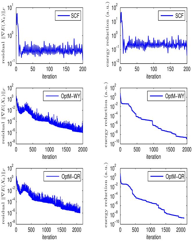
Fig. 1: Residuals $\|\nabla E(X_{k})\|_{F}$ and the energy reduction $E(X_{k})-E_{min}$ of SCF, OptM-WY and OptM-QR on $C_{120}$.

Table 1 also shows that OptM-QR is faster than OptM-WY on most test problems. We next illustrate their convergence behavior using three different tolerances $\varepsilon_{g}=10^{-5},10^{-6}$ and $10^{-7}$ on alanine chain and $C_{120}$ molecules. The results are reported in Table 2. It follows from Tables 1 and 2 that the gradient type methods can often attain a highly accurate solution and OptM-QR behaves slightly better than OptM-WY, especially on large systems.

solver	$\varepsilon_{g}$	$\Delta E_{0}$(a.u.)	Iter	resi	cpu(s)
alanine chain$\quad p=132\quad n=293725$ $cores=32$
OptM-WY	1e-05	1.44e-08	1652	7.80e-06	881
OptM-QR	1e-05	3.50e-08	1199	9.30e-06	606
OptM-WY	1e-06	5.82e-10	2082	9.64e-07	1102
OptM-QR	1e-06	1.73e-10	1413	5.57e-07	712
OptM-WY	1e-07	1.66e-10	2814	9.72e-08	1921
OptM-QR	1e-07	1.65e-10	2016	9.17e-08	1474
$C_{120}\quad p=240\quad n=354093$ $cores=32$
OptM-WY	1e-05	3.18e-08	1537	9.34e-06	1861
OpyM-QR	1e-05	6.91e-08	1383	9.42e-06	1506
OptM-WY	1e-06	1.88e-09	1964	9.73e-07	2339
OptM-QR	1e-06	2.06e-09	2062	9.95e-07	2213
OptM-WY	1e-07	1.23e-09	2776	9.90e-08	4433
OptM-QR	1e-07	1.23e-09	3020	9.97e-08	4261

Table 2: Numerical results with respect to different $\varepsilon_{g}$.

We next examine parallel scalability of all three methods. For brevity, we only show results for the systems: $C_{60}$, alanine chain, 2JMO and fasciculin2. Let $k_{0}$ be the smallest number of cores so that the required memory for the given problem can fit in these cores. The speedup factor for running a code on $k$ cores is defined as

(4.35) $$\mbox{speedup-factor}(k_{0},k)=\frac{\mbox{wall clock time for a $k_{0}$-core run}}{\mbox{wall clock time for a $k$-core run}}.$$

When the wall clock time is measured, we only run 10 iterations for SCF and 100 iterations for OptM-WY and OptM-QR since the parallel speedup factor should not change if more iterations are preformed. The wall clock time for each algorithm is split into two parts. The part, denoted by T0, involves the calculation of the total energy, gradients and Hamiltonian, which are determined by the specific implementation of Octopus. For example, the calculation of gradients uses the subroutine “Hamiltonian_apply” and the update of Hamiltonian uses the subroutines “density_calc” and “v_ks_calc”. The calculation of the total energy uses a revision of the origin subroutine “total_energy” by setting the parameter “full” to be “.ture.” and then summing up all energy terms. All other wall clock time is counted as T1, which reflects the algorithmic difference among different algorithms.

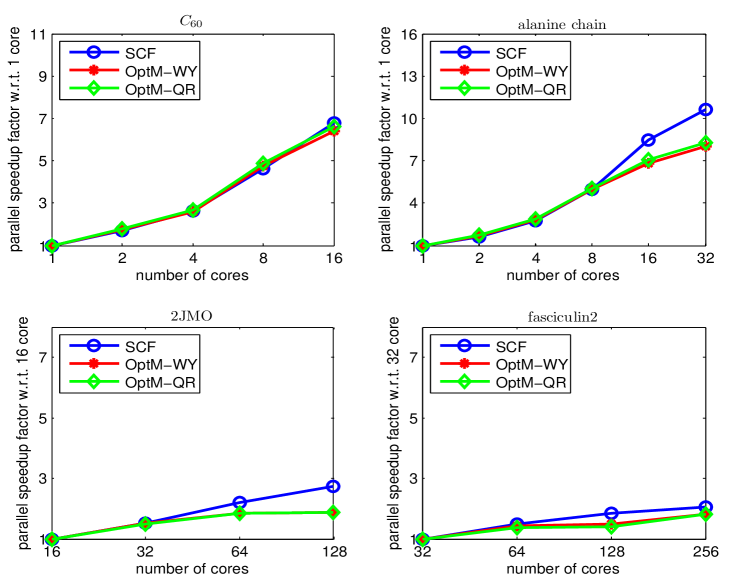
Fig. 2: The speedup factor with respect to T0

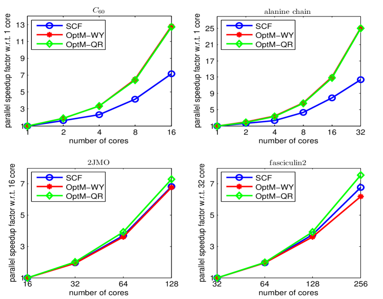
Fig. 3: The speedup factor with respect to T1

Figures 2 and 3 show the speedup factors of T0 and T1, respectively. We can see that the scalability of T0 is not good on 2JMO and fasciculin2. The performance of SCF is not always the same as the gradient type methods because that their time and proportion of calculating the total energy, gradients and Hamiltonian are different. On the other hand, OptM-QR is better than SCF in terms of T1. OptM-WY behaves similar to OptM-QR on $C_{60}$ and alanine chain, but it is worse on 2JMO and fasciculin2. The reason is that the complexity at each iteration also depends on the number of columns $p$. The Cholesky factorization of a $p\times p$ matrix in OptM-QR costs $\frac{1}{3}p^{3}$ while the calculation of $\left(I+\frac{\tau}{2}V^{\top}U\right)^{-1}V^{\top}X$ in OptM-WY needs $\frac{40}{3}p^{3}+\mathcal{O}(p^{2})$. These two operations are not parallelized in our current implementation. Consequently, OptM-QR has a slightly higher parallel speedup factor than OptM-WY. We next present the ratio $T_{0}/(T_{0}+T_{1})$ in Figure 4. It shows that the most time consuming part of SCF is T1, in particular, for larger systems, due to the eigenvalue computation. On the other hand, T0 accounts for a large proportion of OptM-QR and OptM-WY. Hence, the scalability of our gradient type methods can be further improved if the efficiency of $T0$ can be enhanced.

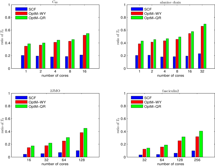
Fig. 4: The ratio of $T_{0}/(T_{0}+T_{1})$.

Finally, we investigate the sensitivity of the gradient type methods with respect to the number of cores on the systems $C_{60}$ and alanine chain. The parameters of each run are the same. The results are presented in Table 3. We can see that the total number of iterations of the gradient type methods are not always the same. The reason may be that the BB step size is sensitive to numerical errors. Hence, a more robust method for choosing the step size is expected.

	OptM-WY			OptM-QR			SCF
cores	resi	Iter	cpu(s)	resi	Iter	cpu(s)	resi	Iter	cpu(s)
$C_{60}\quad p=120\quad n=191805$ $\varepsilon_{g}\,=\,1e-6$
1	9.96e-07	226	904	7.89e-07	245	891	7.05e-07	23	1649
2	6.79e-07	260	562	8.79e-07	244	484	6.67e-07	23	1123
4	6.37e-07	224	294	9.97e-07	241	291	6.67e-07	23	672
8	3.72e-07	237	165	9.51e-07	236	153	6.52e-07	23	376
16	5.68e-07	239	100	9.53e-07	242	96	6.51e-07	23	225
alanine chain$\quad p=132\quad n=293725$ $\varepsilon_{g}\,=\,1e-6$
1	9.93e-07	1605	11984	9.95e-07	1591	10671	–	–	–
2	9.75e-07	2086	8534	7.59e-07	1949	7475	–	–	–
4	9.50e-07	1856	4344	9.75e-07	1584	3442	–	–	–
8	9.06e-07	1985	2526	9.97e-07	1502	1760	–	–	–
16	9.98e-07	1816	1410	8.72e-07	1828	1318	–	–	–
32	9.64e-07	2082	1123	5.57e-07	1413	727	–	–	–

Table 3: Numerical results with respect to the number of cores. The results of SCF are not reported for alanine chain because SCF failed as shown in Table 1 .

4.2 Numerical results for the OFDFT model

Our numerical analysis for OFDFT is based on aluminum crystal, where (2.4) is used as KEDF and external potential is the GNH (Goodwin-Needs-Heine) pseudopotential [19]:

(4.36) $$V_{ext}(r)=\frac{2}{\pi}\int_{0}^{\infty}\frac{\sin(rt)}{rt}\Big{(}(Z-AR)\cos(Rt)+A\frac{\sin(Rt)}{t}\Big{)}e^{-(\frac{t}{R_{c}})^{6}}dt,$$

where $Z$ is the number of valence electrons, $R=1.15$, $R_{c}=3.5$ and $A=0.1107$. Several finite systems with fixed atomic positions are simulated.

We compare the performance of SCF, OptM-WY and OptM-QR. They are further embedded in the adaptive mesh refinement method Algorithm 4. Since OFDFT is not available in Octopus, we implement all methods in the package RealSPACES, which is developed based on the platform PHG (Parallel Hierarchical Grid) [37]. The initial guess is generated by the pseudo-wave functions of aluminum and the initial mesh is produced by RealSPACES. A lattice spacing of 7.559 a.u. is used for the size of the unit cell. The maximum number of iterations for SCF and OptM-QR and OptM-WY is 25 and 200, respectively. We terminated all methods if $\|\nabla E(X_{k})\|_{F}\leq\varepsilon_{g}=10^{-5}$.

A summary of numerical results is reported in Table 4, where $size$, $N_{Al}$, $E^{0}_{p}$, and $E_{b}$ stand for the number of unit cells, the total number of aluminum atoms, the ground state energy per atom, and the binding energy. The binding energy is evaluated by $E_{b}=\frac{E_{0}-N_{Al}E_{s}}{N_{Al}}$, where $E_{0}$ is the ground state energy calculated by (2.6), and $E_{s}=-52.800704(eV)$ is the energy for single aluminum atom. $E^{0}_{p}$, $E_{b}$ and $E_{0}$ are all measured in eV. The number $n$ denotes the total number of degrees of freedom in the final adaptive step.

solver	$E^{0}_{p}$(eV)	$E_{b}$(eV)	$n$	cpu(s)
$size=4\times 4\times 4$ $N_{Al}=365$  $cores=32$
SCF	-57.036037	-4.235333	835908	1557
OptM-WY	-57.036037	-4.235333	835904	867
OptM-QR	-57.036038	-4.235334	835895	756
$size=7\times 7\times 7$ $N_{Al}=1688$  $cores=64$
SCF	-57.150302	-4.349598	4486542	8368
OptM-WY	-57.150302	-4.349598	4485928	5245
OptM-QR	-57.150302	-4.349598	4485919	4732
$size=10\times 10\times 10\quad N_{Al}=4631$  $cores=128$
SCF	-57.628512	-4.827808	13411386	15588
OptM-WY	-57.628513	-4.827809	13411388	9412
OptM-QR	-57.628513	-4.827809	13411373	8852
$size=12\times 12\times 12$ $N_{Al}=7813$  $cores=128$
SCF	-58.093705	-5.293001	45010875	58678
OptM-WY	-58.093706	-5.293003	45010864	30645
OptM-QR	-58.093707	-5.293003	45010826	26457

Table 4: Numerical results computed by the adaptive mesh refinement method.

Table 4 shows that the ground state energy per atom converges as the size of the system is increased. The gradient type methods are more efficient than SCF, and OptM-QR is slightly better than OptM-WY. We should point out there exists difference on the wave functions on the adaptive grids obtained from different gradient type methods. Hence, the final total number of degrees of freedom $n$ may be different even if their “size” are the same.

The change of the residuals versus the iteration history on a particular mesh is presented in Figure 5 for systems $Al_{1688}$ and $Al_{4631}$, respectively, where $Al_{1688}$ denotes the aluminum $7\times 7\times 7$ cluster with 1688 aluminum atoms and similar notations are used for $Al_{365}$, $Al_{4631}$ and $Al_{7813}$. The gradient type methods are able to reduce the residuals steadily although they may be increased at some iterations. The contours of the ground state charge density and their corresponding adaptive mesh distributions are shown in Figure 6 for an intuitive illustration of our approaches.

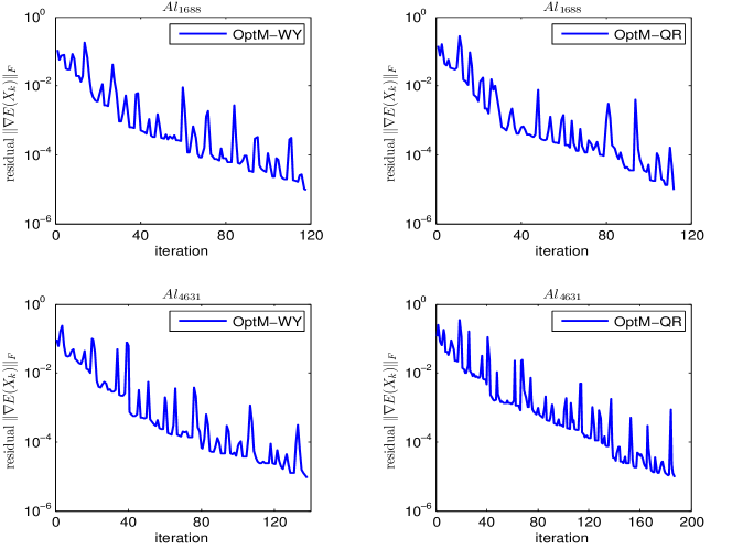
Fig. 5: Residuals $\|G-XG^{T}X\|_{F}$. Top: $Al_{1688}$; Bottom: $Al_{4631}$.

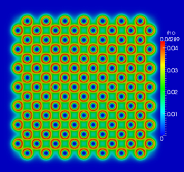
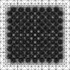
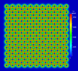
Fig. 6: (a) and (c) are the contours of the ground state charge density at plane $z=0$ for $Al_{1688}$ and $Al_{4631}$, respectively. (b) and (d) are the corresponding adaptive mesh distribution of (a) and (c), respectively.

We next examine the parallel scalability of the gradient type methods. Similar to KSDFT, the wall clock time is split into the T0 and T1 parts, where T0 includes the wall clock time on computing the total energy, gradients and Hamiltonian, while all other wall clock time is counted as T1. The speedup factors of T0 and T1 defined in (4.35) for systems $Al_{365}$ and $Al_{1688}$ are presented in Figures 7 and 8, respectively. We can see that the difference between OptM-WY and OptM-QR is small. The reason is that the parallel scalability of each method only depends on the spatial degrees of freedom $n$ in the case of $p=1$. The difference between T0 and T1 is also small. Consequently, the overall parallel scalability is high. The performance of OptM-WY and OptM-QR is at least comparable to that of SCF.

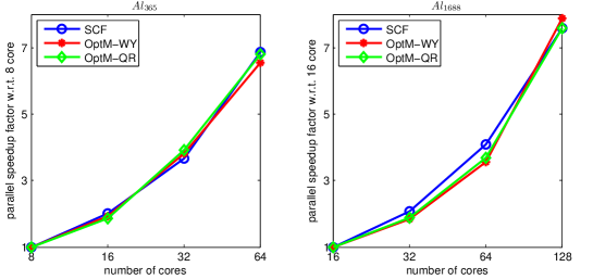
Fig. 7: The speedup factors for aluminum crystal with respect to T0.

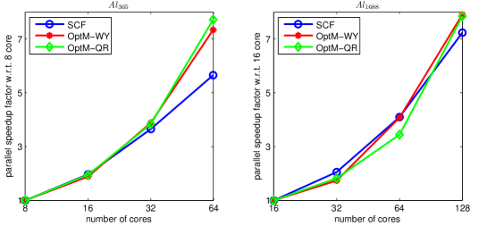
Fig. 8: The speedup factors for aluminum crystal with respect to T1.

Finally, the results obtained by refining the mesh uniformly are presented in Table 5. This strategy uses the same number of meshes as the adaptive mesh refinement method in Table 4, but these meshes are refined uniformly from their coarser levels. We can conclude from these two tables that the adaptive mesh refinement strategy can greatly reduce the total number of degrees of freedom as well as the computational cost.

solver	$E^{0}_{p}$(eV)	$E_{b}$(eV)	$n$	cpu(s)
$size=4\times 4\times 4$ $N_{Al}=365$  $cores=32$
OptM-WY	-57.092410	-4.291706	1432850	1448
OptM-QR	-57.092441	-4.291737	1432850	1288
$size=7\times 7\times 7$ $N_{Al}=1688$  $cores=64$
OptM-WY	-57.151769	-4.351065	16974593	20688
OptM-QR	-57.151767	-4.351063	16974593	17356
$size=10\times 10\times 10\quad N_{Al}=4631$  $cores=128$
OptM-WY	-57.784717	-4.984013	37991437	19347
OptM-QR	-57.784860	-4.984156	37991437	18362

Table 5: Numerical results computed by the uniformly mesh refinement method

5 Concluding remarks

In this paper, we study gradient type methods for solving the KSDFT and OFDFT models in electronic structure calculations. Unlike the commonly used SCF iteration, these approaches do not rely on solving linear eigenvalue problems. The main components of our approaches are gradients on the Stiefel manifold and operations for preserving the orthogonality constraints. They are cheaper and often have better parallel scalability than eigenvalue computation. A specific form uses the QR factorization to orthogonalize the gradient step on the Stiefel manifold explicitly. To the best of the authors’ knowledge, it is the first time that the QR-based method is systematically studied for electronic structure calculations. The gradient methods is further improved by the state-of-the-art acceleration techniques such as Barzilai-Borwein steps and non-monotone line search with global convergence guarantees. We implement our methods based on two real space software packages, i.e., Octopus for KSDFT and RealSPACES for OFDFT, respectively. Numerical experiments show that our methods can be more efficient and robust than SCF on many instances. Their parallel efficiency is ideal as long as the evaluation of the total energy functional and their gradients is efficient. We believe that these methods are powerful techniques in simulating large and complex systems.

References

- [1] Abinit. http://www.abinit.org.
- [2] P.-A. Absil, R. Mahony, and R. Sepulchre, Optimization Algorithms on Matrix Manifolds, Princeton University Press, Princeton, NJ, 2008.
- [3] D. G. Anderson, Iterative procedures for nonlinear integral equations, J. Assoc. Comput. Mach., 12 (1965), pp. 547–560.
- [4] J. Barzilai and J. M. Borwein, Two-point step size gradient methods, IMA J. Numer. Anal., 8 (1988), pp. 141–148.
- [5] S. A. Beasley, V. A. Hristova, and G. S. Shaw, Structure of the parkin in-between-ring domain provides insights for e3-ligase dysfunction in autosomal recessive parkinson’s disease, Proc. Natl. Acad. Sci., 104 (2007), pp. 3095–3100.
- [6] P. Bendt and A. Zunger, New approach for solving the density-functional self-consistent-field problem, Phys. Rev. B., 26 (1982), pp. 3114–3137.
- [7] Y. Bourne, P. Taylor, and P. Marchot, Acetylcholinesterase inhibition by fasciculin: crystal structure of the complex, Cell., 83 (1995), pp. 503–512.
- [8] K. M. Carling and E. A. Carter, Orbital-free density functional theory calculations of the properties of Al, Mg, and Al-Mg crystalline phases, Model. Simulat. Mater. Sci. Eng., 11 (2003), pp. 339–348.
- [9] J. R. Chelikowsky, N. Troullier, and Y. Saad, Finite-difference-pseudopotential method: Electronic structure calculations without a basis, Phys. Rev. L., 72 (1994), pp. 1240–1243.
- [10] H. Chen, X. Gong, L. He, Z. Yang, and A. Zhou, Numerical analysis of finite dimensional approximations of Kohn-Sham models, Adv. Comput. Math., 38 (2013), pp. 225–256.
- [11] H. Chen, L. He, and A. Zhou, Finite element approximations of nonlinear eigenvalue problems in quantum physics, Comput. Methods Appl. Mech. Engrg., 200 (2011), pp. 1846–1865.
- [12] H. Chen, X. Gong, and A. Zhou, Numerical approximations of a nonlinear eigenvalue problem and applications to a density functional model, Math. Meth. Appl. Sci., 33 (2010), pp. 1723–1742.
- [13] X. Dai, X. Gong, Z. Yang, D. Zhang, and A. Zhou, Finite volume discretizations for eigenvalue problems with applications to electronic structure calculations, Multi. Model. Simul., 9 (2011), pp. 208–240.
- [14] J. Fang, X. Gao, and A. Zhou, A Kohn-Sham equation solver based on hexahedral finite elements, J. Comp. Phys., 231 (2012), pp. 3166–3180.
- [15] J. B. Francisco, J. M. Martinez, and L. Martinez, Globally convergent trust-region methods for self-consistent field electronic structure calculations, J. Chem. Phys., 121 (2004), pp. 10863–10878.
- [16] J. B. Francisco, J. M. Martínez, and L. Martínez, Density-based globally convergent trust-region methods for self-consistent field electronic structure calculations, J. Math. Chem., 40 (2006), pp. 349–377.
- [17] GAUSSIAN. http://www.gaussian.com/
- [18] X. Gong, L. Shen, D. Zhang, and A. Zhou, Finite element approximations for Schrödinger equations with applocations to electronic structure computations, J. Comput. Math., 26 (2008), pp. 310–323.
- [19] L. Goodwin, R. J. Needs, and V. Heine, A pseudopotential total energy study of impurity-promoted intergranular embeittlement, J.Phys.: Condens. Matter, 2 (1990), pp. 351–365.
- [20] K. Hirose, T. Ono, Y. Fujimoto, and S. Tsukamoto, First-Principles Calculations in Real-Space Formalism, Imperial College Press, 2005.
- [21] G. Ho, C. Huang, and E. A. Carter, Describing metal surfaces and nanostructures with orbital free density functional theory, Curr. Opin. Solid State Mater. Sci., 11 (2008), pp. 57–61.
- [22] H. Jiang, H. U. Baranger, and W. Yang, Density-functional theory simulation of large quantum dots, Phys. Rev. B., 165 (2003), 165337.
- [23] D. D. Johnson, Modified Broyden’s method for accelerating convergence in self-consistent calculations, Phys. Rev. B., 38 (1988), pp. 12807–12813.
- [24] W. Kohn and L. J. Sham, Self consistent equations including exchange and correlation effects, Phys. Rev. A., 140 (1965), pp. 1133–1138.
- [25] G. Kresse and J. Furtthmüller, Efficiency of ab initio total energy calculations for metals and semiconductors using a plane wave basis set, Comput. Mater. Sci., 6 (1996), pp. 15–50.
- [26] X. P. Li, R. W. Nunes, and D. Vanderbilt, Density-matrix electronic-structure method with linear system-size scaling, Phys. Rev. B., 47 (1993), pp. 10891–10894.
- [27] S. A. Losilla and D. Sundholm, A divide and conquer real-space approach for all-electron molecular electrostatic potentials and interaction energies, J. Chem. Phys., 136 (2012), 214104.
- [28] R. M. Martin, Electronic strucutre: Basic Theory and Practical Methods, Unicersity Press, Cambridge, 2004.
- [29] J. M. Millam and G. E. Scuseria, Linear scaling conjugate gradient density matrix search as an alternative to diagonalization for first principles electronic structure calculations, J. Chem. Phys., 106 (1997), pp. 5569–5577.
- [30] P. Motamarri, M. R. Nowak, K. Leiter, J. Knap, and V. Gavini, Higher-order adaptive finite-element methods for Kohn-Sham density functional theory, J. Comp. Phys., 253 (2013), pp. 308-343.
- [31] Octopus. http://www.tddft.org/programs/octopus.
- [32] J. E. Pask and P. A. Sterne, Finite element methods in ab initio electronic structure calculations. Model. Simul. Mater. Sci. Eng., 13 (2005), pp. 71-96.
- [33] M. C. Payne, M. P. Teter, D. C. Allan, T. A. Arias, and J. D. Joannopoulos, Iterative minimization techniques for ab initio total-energy calculations: molecular dynamics and conjugate gradients, Rev. Mod. Phys., 64 (1992), pp. 1045–1097.
- [34] J. P. Perdew and K. Burke, Comparison shopping for a gradient-corrected density functional, Int. J. Quant. Chem., 57 (1996), pp. 309–319.
- [35] J. P. Perdew and Y. Wang, Accurate and simple analytic representation of the electron-gas correlation energy: Generalized gradient approximation, Phys. Rev. B., 45 (1992), pp. 133244–132249.
- [36] B. G. Pfrommer, J. Demmel, and H. Simon, Unconstrained energy functionals for electronic structure calculations, J. Chem. Phys., 150 (1999), pp. 287 – 298.
- [37] PHG. http://lsec.cc.ac.cn/phg/.
- [38] P. Pulay, Convergence acceleration of iterative sequences: the case of SCF iteration, Chem. Phys. Lett., 73 (1980), pp. 393–398.
- [39] Y. Saad, J. R. Chelikowshy, and S. M. Shontz, Numerical methods for electronic structure calculations of materials, SIAM Rev., 52 (2010), pp. 3-54.
- [40] Y. Saad, A. Stathopoulos, J. Chelikowsky, K. Wu, and S. Ogut, Solution of large eigenvalue problems in electronic structure calculation, BIT., 361 (1996), pp. 563–578.
- [41] V. Schauer and C. Linder, All-electron Kohn-Sham density functional theory on hierarchic finite element spaces, J. Comp. Phys., 250 (2013), pp. 644-664.
- [42] SIESTA. http://icmab.cat/leem/siesta/.
- [43] L. Thogersen, J. Olsen, D. Yeager, P. Jorgensen, P. Salek, and T. Helgaker, The trust-region self-consistent field method: Towards a black-box optimization in Hartree–Fock and Kohn–Sham theories, J. Chem. Phys., 121 (2004), pp. 16–27.
- [44] T. Torsti, T. Eirola, J. Enkovaara, T. Hakala, P. Havu, V. Havu, T. Höynälänmaa, J. Ignatius, M. Lyly, I.Makkonen, T. T. Rantala, J. Ruokolainen, K. Ruotsalainen, E. Räsänen, H. Saarikoski, and M. J. Puska, Three real-space discretization techniques in electronic structure calculations. Phys. Stat. Sol., 243 (2006), pp. 1016-1053.
- [45] N. Troullier and J. L. Martins, Efficient pseudopotentials for plane-wave valvulations, Phys. Rev. B., 43 (1991), pp. 1993-2006.
- [46] E. Tsuchida and M. Tsukada, Electronic-structure calculations based on the finite element, Phys. Rev. B., 52 (1995), pp. 5573-5578.
- [47] T. Van Voorhis and M. Head-Gordon, A geometric approach to direct minimization, Molecular Physics., 100 (2002), pp. 1713–1721.
- [48] VASP. http://www.vasp.at/.
- [49] L. Wang and M. P. Teter, Kinetic energy density functional theory, Phys. Rev. B., 45 (1992), pp. 13196–13220.
- [50] Y. A. Wang, N. Govind, and E. A. Carter, Orbital-free kinetic energy density functionals with a density dependent kernel, Phys. Rev. B., 60 (1999), pp. 16350–16358.
- [51] Z. Wen, A. Milzarek, M. Ulbrich, and H. Zhang, Adaptive regularized self-consistent field iteration with exact hessian for electronic structure calculation, SIAM J. Sci. Comput., 35 (2013), pp. A1299–A1324.
- [52] Z. Wen and W. Yin, A feasible method for optimization with orthogonality constraints, Math. Program. Ser. A., (2012).
- [53] C. Yang, J. C. Meza, L. Bee, and L. Wang, KSSOLV-a MATLAB toolbox for solving the Kohn-Sham equations, ACM Trans. Math. Softw., 36 (2009), pp. 1-35.
- [54] C. Yang, J. C. Meza, and L. Wang, A trust region direct constrained minimization algorithm for the Kohn-Sham equation, SIAM J. Sci. Comput., 29 (2007), pp. 1854–1875.
- [55] B. Jiang and Y. Dai, A framework of constraint preserving update schemes for optimization on Stiefel manifold, arXiv:1301.0172, (2012).
- [56] D. Zhang, L. Shen, A. Zhou, and X. Gong, Finite element method for solving Kohn-Sham equations based on self-adaptive terahedral mesh, Phy. Lett. A., 372 (2008), pp. 5071-5076.
- [57] A. Zhou, An anslysis of finite-dimensional approximations for the ground state solution of Bose-Einstein condensates, Nonlinearity., 17, (2004), pp. 541-550.
- [58] A. Zhou, Finite dimensional approximations for the electronic ground state solution of a molecular system, Math. Methods Appl. Sci., 30 (2007), pp. 429–447.
- [59] Y. Zhou, Y. Saad, M. L. Tiago, and J. R. Chelikowsky, Self-consistent-field calculations using Chebyshev-filtered subspace iteration, J. Comp. Phys., 219 (2006), pp. 172–184.