A Challenging Solar Eruptive Event of 18 November 2003 and the Causes of the 20 November Geomagnetic Superstorm. II. CMEs, Shock Waves, and Drifting Radio Bursts

Abstract

We continue our study (Grechnev et al. (2013), doi:10.1007/s11207-013-0316-6; Paper I) on the 18 November 2003 geoffective event. To understand possible impact on geospace of coronal transients observed on that day, we investigated their properties from solar near-surface manifestations in extreme ultraviolet, LASCO white-light images, and dynamic radio spectra. We reconcile near-surface activity with the expansion of coronal mass ejections (CMEs) and determine their orientation relative to the earthward direction. The kinematic measurements, dynamic radio spectra, and microwave and X-ray light curves all contribute to the overall picture of the complex event and confirm an additional eruption at 08:07 – 08:20 UT close to the solar disk center presumed in Paper I. Unusual characteristics of the ejection appear to match those expected for a source of the 20 November superstorm but make its detection in LASCO images hopeless. On the other hand, none of the CMEs observed by LASCO seem to be a promising candidate for a source of the superstorm being able to produce, at most, a glancing blow on the Earth’s magnetosphere. Our analysis confirms free propagation of shock waves revealed in the event and reconciles their kinematics with “EUV waves” and dynamic radio spectra up to decameters.

1 Introduction

The geomagnetic storm on 20 November 2003 with Dst $=-422$ nT was the strongest one after the destructive superstorm on 13 – 14 March 1989 (Dst $=-589$ nT) and has not been surpassed since. The causes of the extreme nature of the 20 November 2003 superstorm and its solar source remain unclear in spite of several attempts to understand them (e.g., Gopal2005; Yermolaev2005; Yurchyshyn2005; Ivanov2006; Moestl2008; Chandra2010; KumarManoUddin2011; Marubashi2012; Cerrato2012, and others). The challenge of this superstorm urged us to investigate into various aspects of the 18 November solar eruptive event in active region (AR) 10501 that is considered to be its only possible source. Eruptions from AR 10501 have been addressed in Paper I [Grechnev et al. (2013)]. Its conclusions are: (i) eruption at 07:29 (all times are referred to UT) produced a missed M1.2 flare probably associated with onset of the first southeast coronal mass ejection, CME1; (ii) eruptions before 07:55 are unlikely to be responsible for the superstorm; (iii) the eruptive filament collided with a topological discontinuity, bifurcated, and transformed into a Y-shaped cloud, which had not left the Sun; thus, the filament should not be directly related to the magnetic cloud hitting the Earth; (iv) one more eruptive episode possibly occurred between 08:07 and 08:17 that could be related to the disintegration of the filament and led to other consequences open to question.

All of the listed studies assumed that the source of the superstorm was either the southeast CME1 observed by the Large Angle and Spectroscopic Coronagraph (LASCO; Brueckner1995) starting from 08:06 or, more probably, the second southwest halo CME (CME2), which appeared at 08:49. According to the model of the cone CME geometry (e.g., Howard1982; FisherMunro1984), the halo shape indicates the earthward (or the opposite) propagation of a CME. Therefore, CME2 has been considered as the major candidate for the source of the superstorm. On the other hand, it is possible that the outer halo of CME2 was a trace of a shock front. If so, then CME2 was not necessarily Earth-directed. Thus, it is necessary to find out the nature of the structural components of CME2 and its actual orientation.

One more challenge of this event is the mismatch between the right-handed helical magnetic cloud (MC) and the pre-eruption region of left-handed helicity established by Chandra2010. To resolve the problem, the authors proposed a right-handed helical ejection from a minor area of AR 10501. Based on this idea, KumarManoUddin2011 related CME1 to a partial eruption at 07:41 from this area and proposed a merger of the magnetic structures of CME1 (presumably right-handed) and CME2. The authors supported the interaction between the CMEs by a drifting radio burst observed by Wind/WAVES around 09:00. Another attempt to understand the encounter of the MC with the Earth based on the conjecture of Chandra2010 was made by Marubashi2012 who considered that the MC evolved from a single right-handed CME. Neither of these studies presented a quantitative confirmation of their conjectures, whilst attributing the superstorm to a partial eruption from a minor region seems to be questionable.

Paper I concluded that CME1 was probably initiated in the east, excessively left-handed, part of AR 10501 at 07:29 (consistent with an estimate of Gopal2005) in association with an unreported M1.2 flare thus contradicting the interpretations of Chandra2010, KumarManoUddin2011, and Marubashi2012. This is why the source region of CME1 is important.

The present paper (Paper II) is focused on CME1 and CME2 and the probable nature of their components. In order to understand their possible geoeffective implications, we in particular address the following questions: when and where was CME1 initiated, how was CME2 directed with respect to the Earth, and what erupted between 08:07 and 08:17 close to the solar disk center. We specify measurements of Gopal2005 and confirm the results by comparing them to signatures of shock waves in dynamic radio spectra at metric and decametric wavelengths as well as their possible near-surface traces. White studying this particular event, we pursue a better understanding of CMEs and related phenomena.

Section 2 describes our measurement techniques. Section 3 outlines the pre-event situation and its overall evolution. Section 4 analyzes the observations. The results are discussed in Section 5 and summarized in Section 6.

2 Measurement Techniques

Two kinds of transients appear in LASCO images: magnetoplasma CME components (henceforth ‘mass ejections’ or ‘CMEs’) and traces of waves (Sheeley2000; Vourlidas2003; Grechnev et al., 2011a; 2011b). The kinematics of the two kinds of transient are different. This section describes kinematics of non-wave and wavelike transients and methods of measurement.

We consider two kinds of wave signatures in LASCO images: faint non-structured (or structured by coronal rays) halo-like outermost envelopes of CMEs and deflections of coronal streamers. The brightness of the halos can be very low. Mass ejections are significantly brighter, with well pronounced loops or threads in their structure. It is difficult to reliably identify both wave signatures and CME structures in a single set of images. We therefore use two separate sets processed in different ways to measure wave traces and mass ejections. For CMEs we use ratios of current LASCO images $C(j)$ to a fixed pre-event image $C(0)$ and limit the values in the ratios from both above and below with thresholds $A_{0}\lsim 1$ and $A_{1}\gsim 1$, $A_{0}<I_{\mathrm{CME}}(j)=C(j)/C(0)<A_{1}$. For wave signatures we use ratios of running differences $C(j)-C(j-1)$ to preceding images $C(j-1)$ also with optimized contrast by adjusting the corresponding thresholds $B_{0}\lsim 0$ and $B_{1}\gsim 0$, $B_{0}<I_{\mathrm{wave}}(j)=[C(j)-C(j-1)]/C(j-1)<B_{1}$.

2.1 Mass Ejections

The kinematics of coronal transients have been measured in several different ways. Height-time plots are obtained by measuring a characteristic CME feature. Then the measurements are differentiated (e.g., Maricic2004; Temmer et al., 2008; 2010). Alternatively, the measurements are fit with an analytic function such as polynomial Yashiro et al. (2004); Gopalswamy et al. (2009), Gaussian Wang, Zhang, and Shen (2009), or more sophisticated models Krall, Chen, and Santoro (2000).

Both approaches should converge to similar results, but each method has its shortcomings. Differentiation of measurements is critical to temporal sampling, errors, and provides large uncertainties. The adequacy of an analytic fit might be questionable. For example, the polynomial fit used in the SOHO LASCO CME Catalog (Yashiro2004; Gopal2009, http://cdaw.gsfc.nasa.gov/CME˙list/) is probably the best way for approximately evaluating the kinematics of CMEs, but the underlying assumption of a constant (or zero) acceleration (i.e., the constancy of the driving/retarding force) does not seem to be realistic. Employment of theoretical models like the flux rope model of Chen (1989; 1996; e.g., KrallChenSantoro2000) is complex, whereas its veracity has not been established.

Our way is based on self-similarity of CME expansion (see, e.g., Illing1984; CremadesBothmer2004). The theory of self-similar expansion of solar CMEs was developed by Low1982. A description of a self-similar expansion convenient for analysis of observations was proposed by Uralov2005. A self-similar expansion of an individual plasma packet under the frozen-field conditions and negligible drag of the medium is described by an equation

$$\rho\frac{d{\bf v}}{dt}=\frac{1}{4\pi}{\bf{rotB\times B}}-{\bf{grad}}{p}-\rho\frac{GM_{\odot}}{r^{2}}{\bf{e}_{\bf{r}}}=\\ {\bf{F}}_{B}+{\bf{F}}_{p}+{\bf{F}}_{g},$$ (1)

where $p$ and $\rho$ are the gas pressure and density; ${\bf B}$ the magnetic field vector, ${\bf v}$ the velocity, $M_{\odot}$ the mass of the Sun, and $G$ the gravitational constant. ${\bf F}_{B}$, ${\bf F}_{p}$, and ${\bf F}_{g}$ are the total magnetic, plasma pressure, and gravitational forces affecting the unit volume. Let $R=R(t)$ be some spatial scale characterizing the size of the expanding region at the instant $t$. The forces in Equation (1) depend on the distance $R$ as

$$|{\bf F}_{B}|\propto\left(\frac{R_{0}}{R}\right)^{4}\frac{1}{R},\quad|{\bf F}_{p}|\propto\left(\frac{R_{0}}{R}\right)^{3\gamma}\frac{1}{R},\quad|{\bf F}_{g}|\propto\left(\frac{R_{0}}{R}\right)^{3}\frac{1}{R^{2}},$$ (2)

where $R_{0}$ is the initial size of the self-similar expansion. Force ${\bf F}_{B}$ combines all magnetic forces affecting the expanding packet including propelling magnetic pressure and retarding magnetic tension. Force ${\bf F}_{p}$ due to plasma pressure is directed outward. The gravitational force ${\bf F}_{g}$ retards expansion. With a polytropic index $\gamma=4/3$, all the terms in Equation (2) which appear in the right-hand-side of Equation (1) decrease synchronously with distance and time by the same scaling factor preserving orientation. This fact determines the self-similar expansion of the ejecta. From the expressions of Uralov2005, the instant velocity $v$ can be related to the distance from the expansion center $R$ Grechnev et al. (2008):

$$v^{2}=v_{0}^{2}+\left(v_{\infty}^{2}-v_{0}^{2}\right)\left({1-R_{0}/R}\right),$$ (3)

where $v=dR/dt$ and $v_{0}$ and $v_{\infty}$ are the initial and asymptotic velocities of the self-similar expansion stage. Analysis of this expression shows the following Grechnev et al. (2011a).

1. Acceleration of the ejecta in self-similar expansion can only decrease by the absolute value or be exactly zero. Therefore, the self-similar approach does not apply to initial stages, when the acceleration increases.

2. Acceleration $a$, if nonzero, goes at large distances ($R\approx r\gg R_{\odot}$) as $|a|\propto r^{-2}\to 0$. Thus, self-similar expansion cannot be fit with any polynomial.

3. Three expansion regimes are possible:

   (a) accelerating ejecta, $v_{0}<v_{\infty}$;

   (b) decelerating ejecta, $v_{0}>v_{\infty}$ (‘explosive’ eruption);

   (c) inertial expansion, $v_{0}=v_{\infty}$.

The accelerating regime (a) probably applies to all non-flare-related CMEs and many flare-related ones. In cases (b) and (c), a strong initial impulsive acceleration occurs before the onset of the self-similar stage.

Integrating Equation (3), despite its simplicity, cannot provide an explicit distance vs. time dependence. The following expression allows one to calculate a self-similar expansion implicitly, as time $t$ vs. the heliocentric distance $r$, given the distance of the eruption center $r_{\mathrm{c}}$ and the CME velocity $v_{1}$ measured at time $t_{1}$ at a distance $r_{1}$:

$$t(r)=t_{1}+1/v_{\infty}^{3}\times\qquad\qquad\qquad$$

$$\left\{Sv_{\infty}\sqrt{r-r_{\mathrm{c}}}-v_{\infty}v_{1}r_{1}+(v_{\infty}^{2}-v_{1}^{2})r_{1}\ln\left[\frac{v_{\infty}\sqrt{r-r_{\mathrm{c}}}+S}{(v_{\infty}+v_{1})\sqrt{r_{1}}}\right]\right\}$$ (4)

$$\mathrm{with}\quad S=\sqrt{v_{\infty}^{2}(r-r_{\mathrm{c}}-r_{1})+v_{1}^{2}r_{1}}.$$

The initial estimates of $v_{1}$ and $v_{\infty}$ can be taken from the CME catalog and improved iteratively. The onset time $t_{0}$ of a self-similar expansion is:

$$t_{0}=\left\{\begin{array}[]{cc}t(r_{\mathrm{c}})&\mathrm{for}\quad v_{1}>v_{\infty},\\ t\left(\left[{r_{\mathrm{c}}+r_{1}\left(1-\frac{v_{1}^{2}}{v_{\infty}^{2}}\right)}\right]\right)&\mathrm{for}\quad v_{1}<v_{\infty}.\end{array}\right.$$ (7)

Monotonically decreasing or zero acceleration is consistent with observations (see, e.g., Zhang2001; ZhangDere2006; Temmer et al., 2008; 2010). Although the self-similar approximation does not apply to the initial impulsive acceleration stage, it promises a better fit to the observed CME expansion and higher accuracy of the estimated onset time than the polynomial fit does.

In specifying the CME onset times we also employ the temporal closeness of the major CME acceleration with hard X-ray (HXR) or microwave bursts revealed in the mentioned series of the papers as well as the Neupert effect Neupert (1968). These circumstances indicate that the CME velocity profile is roughly reflected in the rising phase of the corresponding soft X-ray light curve recorded with GOES.

2.2 Waves

CME-associated waves are most likely excited by abrupt eruptions of magnetic ropes inside developing CMEs during rising hard X-ray and microwave bursts Grechnev et al. (2011a). The waves rapidly steepen into shocks, pass through the forming CME frontal structures, and freely propagate afterwards for some time like decelerating blast waves (cf. PomoellVainioKissmann2008). The corresponding quantitative description allows one to reconcile manifestations of shocks in different emissions including Moreton waves, ‘EUV waves’, metric type II bursts, and leading edges of CMEs. A narrowband harmonic type II burst appears if the shock front compresses the current sheet of a coronal streamer, producing a running flare-like process Uralova and Uralov (1994).

A simple model (Grechnev et al. 2008; 2011a; 2011b) describes propagation of such a blast-like shock wave in plasma with a radial power-law density falloff $\delta$ from an eruption center, $n=n_{0}(x/h_{0})^{-\delta}$. Here $x$ is the distance and $n_{0}$ is the density at a distance of $h_{0}\approx 100$ Mm, which is close to the scale height. The propagation of a shock wave in the self-similar approximation is determined by plasma density distribution, being almost insensitive to the magnetic fields. Such a wave decelerates if $\delta<3$, due to a growing mass of swept-up plasma. Propagation of such a shock vs. time $t$ is described by an expression $x(t)\propto t^{2/(5-\delta)}$, which is more convenient for use in a form

$$x(t)=x_{1}[(t-t_{0})/(t-t_{1})]^{2/(5-\delta)},$$ (8)

where $t$ and $x$ are the current time and distance, $t_{0}$ is the wave onset time, and $t_{1}$ and $x_{1}$ correspond to one of the measured fronts.

To fit the drift of a type II burst, we take an initial estimate of $\delta$ (typically $2\leq\delta\leq 2.8$) and choose a reference point on a band with a harmonic number $N_{\mathrm{ref}}$ (1 or 2) at a frequency $f_{\mathrm{ref}}$ and time $t_{1}$. The corresponding plasma density is $n_{1}=[f_{\mathrm{ref}}(t_{1})N_{\mathrm{ref}}^{-1}/(9\times 10^{3})]^{2}$, and the height is $x_{1}=h_{0}\,(n_{0}/n_{1})^{1/\delta}$. Then the height – time plot of the shock tracer is calculated from Equation (8); the corresponding density variation is $n(t)=n_{0}\,[x(t)/h_{0}]^{-\delta}$. The trajectory of the fundamental-emission type II band is $f_{\mathrm{fund}}(t)=9\times 10^{3}[n(t)]^{1/2}$, and the trajectory of the harmonic-emission band is $f_{\mathrm{harm}}(t)=2f_{\mathrm{fund}}(t)$. By adjusting $\delta$ and $t_{0}$ in sequential attempts, we approach a best trajectory of the bands Grechnev et al. (2011a). The spectrum can be reconciled with measured heights by adjusting $n_{0}$, as usually done.

Presumed traces of shocks in coronagraph images are fitted similarly. Input parameters are starting estimates of $\delta$ and $t_{0}$, the heliocentric distances of the wave origin $r_{0}$ and the wave front $r_{1}$ measured at a time $t_{1}$. The initial approximation of the height – time plot is $r(t)=(r_{1}-r_{0})\left[(t-t_{0})/(t_{1}-t_{0})\right]^{2/(5-\delta)}+r_{0}$. Then a best fit is achieved in sequential attempts (Grechnev et al. 2011a; 2011b).

2.3 Resizing Representation

CMEs are usually analyzed by using images in which the spatial resolution is fixed so that the Sun has the same size, while a CME expands. Self-similarity of CME expansion can be used to improve the accuracy of measurements. We adjust the spatial scale to fix the CME size. This way reveals properties of CME expansion that are difficult to notice in the usual representation.

We resize images according to a corresponding fit described in the preceding sections to compensate expansion of a transient and keep its visible size unchanged. In each of the resized images we outline the whole transient with an oval by changing its parameters according to an analytic fit and endeavor to catch the outer contour. Fitting the whole transient rather than single feature considerably improves the accuracy, and resizing all of the images by a single fit allows us to neglect minor irregular deviations between sequential images. Small systematic trends can be detected and compensated for in looking at a movie composed from resized images. Measurement accuracy can be farther improved in this way.

The resizing representation also (i) facilitates detection of deviations in expansion of CME components from a self-similar one providing indications of their nature and revealing internal motions in a CME, (ii) allows measurements from CME flanks when its leading edge departs from the field of view; (iii) simplifies identification of CME components visible in white light with structures observed in different emissions at earlier stages of an eruption.

From the kinematics of CMEs and shock waves it follows that a CME asymptotically approaches a fixed velocity, while a related shock wave continuously decelerates. The relative distance between a fast CME and the shock front decreases so that eventually it enters the bow-shock regime. This probably occurs beyond the field of view of LASCO-C3, while the approach of a CME to the leading wave front is sometimes visible in resized images. If a CME is not fast enough, then the shock decays to a weak fast-mode disturbance.

3 Overview of the Event

3.1 Pre-event Situation

The pre-event situation is presented in Figure 1. The H$\alpha$ image in Figure 1a (Kanzelhöhe Solar Observatory, KSO) shows a large U-shaped filament F1 rooted in AR 10501 and pointed southwest. The pre-eruption filament was inclined to the solar surface by $\approx 60^{\circ}$ ($\approx 23^{\circ}$ to the line of sight, see Paper I). The green contours show the neutral line of the line-of-sight magnetic component ($B_{l}$) at the photospheric level. The green contours are rather coarse tracers mainly corresponding to dark filaments F1, F2, and F3 in the H$\alpha$ image, but deviating considerably from a high-latitude southeast filament.

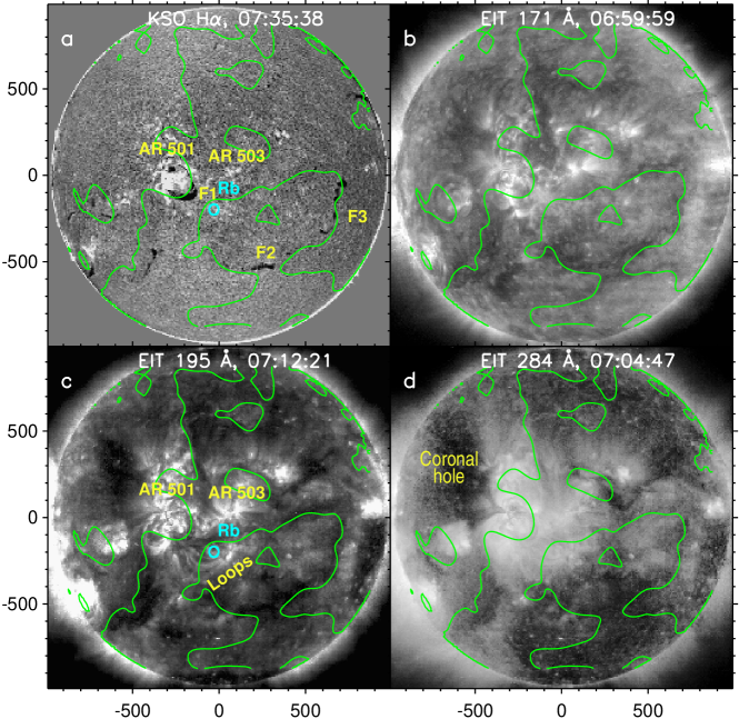
Figure 1.: Pre-event situation in a KSO H$\alpha$ image (a) and EIT images at 171 Å (b), 195 Å (c), and 284 Å (d). The green contours present the magnetic neutral line. F1 is the pre-eruption main filament, F2 an F3 are remote filaments. The light-blue oval marks region Rb where the eruptive filament bifurcated. The axes show the coordinates in arcsec from the solar disk center.

Southwest neighbors of AR 10501 were AR 10503 and region ‘Rb’ (small light-blue oval) where eruptive filament F1 bifurcated. Long loops labeled in Figure 1c south from region Rb connected a western plage region with the south edge of AR 10501. Figures 1b and 1c show that filaments F2 and F3 visible in Figure 1a were arranged along an extended channel still farther southwest. The propagation of shock waves excited by eruptions could be affected by density inhomogeneities indicated by brighter regions by the sides of the filaments as well as a large coronal hole northeast of AR 10501 in Figure 1d (EIT 284 Å; Delab1995).

3.2 Time Profiles and Episodes of the Whole Event

Figure 2 presents time profiles of soft (a, b) and hard (c) X-ray emissions as well as microwaves (d) for the whole event. The GOES soft X-ray (SXR) light curves are supplied with comments on their importance, positions of the flares, and onset times of the CMEs estimated by Gopal2005 and specified below. A detailed description is given in Paper I.

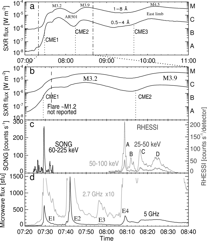
Figure 2.: Flare emissions throughout the whole event. (a) GOES SXR flux; (b) its extended part in the interval marked with dash-dotted lines in panel (a); (c) hard X-ray flux; (d) microwaves at 5 GHz (black) and 2.7 GHz (gray, magnified by a factor of 10).

Table 1 lists associations of the flare peaks E1 – E4 with eruptive episodes according to Paper I. Episode E1 with strong impulsive HXR and microwave bursts increased the SXR flux up to $\approx\,$M1.2 level but was not reported as a separate event. After E1, H$\alpha$ flare ribbons, a flare arcade, and EUV dimmings have appeared. This episode is a candidate for the onset of CME1, but a related eruption was not observed (TRACE had a gap in observations). This caused confusion about the onset time of CME1 in some preceding studies.

Table 1.: Episodes of eruption in AR 10501 revealed in Paper I.

Episode	Peak time	Manifestation
E1	07:29	Eruption in the east part of AR 10501. Unreported M1.2 flare
E2	07:41	Impulsive jet-like ejection. Main filament F1 departs
E3	07:56	Main filament F1 accelerates
E4A	08:09	Eruptive filament F1 collides with region of bifurcation
E4B	08:12	Eruptive filament F1 bifurcates
E4C	08:16	Region of bifurcation dims and disconnects from AR 10501
E4D	08:24	Last flare episode (not considered in Paper I)
–	08:23 – 09:55	Remnants of filament F1 move toward the limb as Y-like cloud

An impulsive jetlike ejection erupted at 07:41 (E2) along the southeast leg of filament F1 and then moved along the loops denoted in Figure 1c. Paper I concluded that development of a CME in episode E2 was unlikely, but the sharp ejection could have produced a shock. The latter conjecture is supported by a type II burst, which was reported by several observatories starting from 07:47.

Filament F1 slowly departed after episode E2 and additionally accelerated to 110 km s^-1 during a weak episode E3. At about 08:07 the eruptive filament collided with region Rb and bifurcated. The collision and subsequent phenomena were manifested in a four-component flare observed in the H$\alpha$ line in KSO, in EUV with TRACE, and in HXR with RHESSI (Miklenic et al. 2007; 2009; Moestl2008). The HXR peaks E4A and E4B (Figure 2c) had a response in the bifurcation region Rb, indicating its connection with the flare site in AR 10501 that later disappeared. Dimming developed in region Rb at that time.

Then the bifurcated filament inverted and transformed into a large dark Y-shaped cloud visible in the CORONAS-F/SPIRIT 304 Å images to move during 08:23 – 09:55 southwest toward the limb. The fastest part of the Y-darkening had a speed of $\approx 210$ km s^-1, and its main body which had an initial speed of 110 km s^-1 decelerated, suggesting an almost constant real speed nearly along the solar surface.

The transformation of the eruptive filament and disconnection of the bifurcation region Rb from AR 10501 suggest one more significant eruption during episodes E4A – E4C. Paper III (Uralov et al., in preparation) will consider what occurred in this region at that time. A later eruption associated with an M4.5 SXR peak at 10:11 (Figure 2a) occurred at the east limb in a rising region 10508 (return of AR 10486). Most likely, this event was related to the third, large CME, whose extrapolated onset time was about 09:40 Gopalswamy et al. (2005).

3.3 CMEs

Figures 3a and 3c show LASCO ratio images of three significant CMEs observed on that day (ChertokGrechnev2005; Grechnev2005; Gopal2005). The EIT 195 Å ratio images in the central insets are magnified by factors 1.45 (a) and 2.68 (b,c) to better show related surface activity. The EIT 195 Å ratio image in Figure 3d presents changes throughout the whole event in AR 10501. CME1 and CME2 were related to this event.

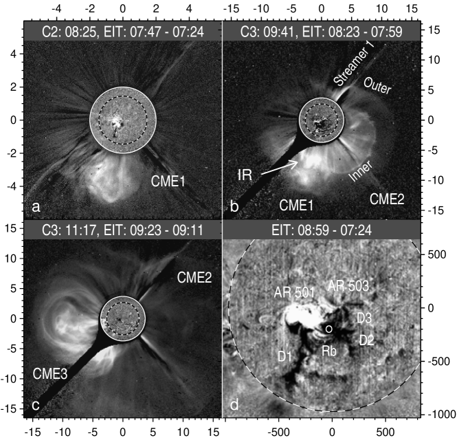
Figure 3.: Three major CMEs of 18 November (a – c) and summary of surface activity in the post-event/pre-event EIT 195 Å ratio image (d). EIT ratio images inserted into the LASCO ratio images are magnified by factors 1.45 (a) and 2.68 (b,c) for better viewing. The solid circles denote the inner boundaries of the fields of view of the coronagraphs. The broken circles denote the solar limb in EIT images. The axes show distances from the solar disk center in solar radii (a – c) and in arcsec (d).

The southeast CME1 (Figure 3a) appeared at 08:06. Its linear-fit speed was 1223 km s^-1. The onset time estimated by Gopal2005 was about 07:22. The volume of CME1 appears to be filled with enhanced-density diffuse material and loop-like structures. The CME structure approximately corresponds on the Sun to an elongated south dimming, a deeper central dimming adjacent to a bright arcade, and the arcade itself. The dimming and flare arcade started to develop before 07:35 according to EUV and H$\alpha$ data (Figure 4 of Paper I) suggesting that the onset time of CME1 was still earlier, most likely, corresponding to the flare episode E1 at 07:29. In addition to the relatively narrow south CME1, its faint partial-halo extension is detectable in the whole eastern half of the image suggesting an expanding wave disturbance.

The brighter, wider and faster southwest CME2 (Figure 3b) appeared at 08:49. Its east flank intruded into CME1 (the intrusion region IR in the figure). The linear-fit speed of the fastest feature of CME2 was 1660 km s^-1. Gopal2005 detected the inner and outer components of CME2 and estimated their onset times of about 08:08 and 08:20, respectively. The structure of CME2 looks different from a three-part one: neither a bright core nor dark cavity separating it from the frontal structure were pronounced. The inner component consisted of radial threadlike features, suggesting that it was an expanding arcade. The faint outer halo component had a diffuse non-structured body and a pronounced leading edge. This halo edge crossed a distorted streamer 1 in Figure 3b well ahead of the inner structure, suggesting an expanding shock wave Sheeley, Hakala, and Wang (2000); Vourlidas et al. (2003); Grechnev et al. (2011a). A large central dimming in regions Rb and AR 10503 in Figure 3b suggests location of a CME source region there.

A large southeast CME3 observed starting from 09:50 (Figure 3c) was not related to AR 10501 (ChertokGrechnev2005; Grechnev2005; Gopal2005). Most likely, CME3 was due to an eruption at the east limb from a rising AR 10508 (former 10486), as an EIT image in the inset shows, and corresponded to an M4.5 SXR flare, which peaked at 10:11 (Figure 2a). The three-part structure of CME3 was preceded by a fast faint halo (the average speed of 1824 km s^-1), which deflected the streamers suggesting one more shock wave. Magnetic structures of CME3 are not expected to have reached the Earth, as preceding studies concluded. The only possible implication of CME3 could be a lateral pressure from the associated shock front to constrain expansion of the magnetic cloud responsible for the 20 November superstorm.

The EIT 195 Å ratio image in Figure 3d shows a bright arcade in AR10501 (which looks saturated, because we show a narrow range of the brightness) and dimmed regions. Dimming D1 developed in association with CME1. Dimming D2 discussed in Paper I developed around region Rb, where the U-shaped filament bifurcated. A star-like dimming D3 also appeared in region 10503 thus indicating its involvement.

4 Coronal Transients Observed During the Event

4.1 CME1 (08:05) and Wave 1

A wide, faint halo-like extension of CME1 suggestive of an expanding wave front is called hereafter wave 1. We fit the observed expansion of the halo by using Equation (8) from Section 2.2 and expansion of the CME1 main structure by using Equations (4) and (7) from Section 2.1. The measurement accuracy cannot be high because of the absence of observations of a related eruption, and therefore we limit our attempts by acceptable correspondence with available data. We use a simpler accelerating kinematics, because it is not possible to recognize whether CME1 accelerated or decelerated at large distances. We also employ the mentioned expectation of similarity between the rising parts of the SXR flux and the CME speed. The kinematical plots are shown in Figure 4. The plots for both CME1 and wave 1 converge to event E1 ($\approx\,$M1.2) at about 07:29. A sharper rise of the SXR emission after 07:34 (the dotted part of the GOES light curve) is due to the next episode E2. The height-time plot of CME1 is close to the measurements in the CME catalog denoted by symbols.

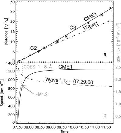
Figure 4.: Kinematical plots of CME1 (solid) and associated wave 1 (dashed) visible in LASCO images in Figures 5 and 6. The symbols in panel (a) present the measurements from the CME catalog. The dotted line in panel (b) presents the GOES SXR flux at 1 – 8 Å.

Figures 5 and 6 allow one to evaluate the quality of the measurements presented in Figure 4. Figure 5 shows the propagation of the faint wave 1 in LASCO images with a highly enhanced contrast. All the images are progressively resized following the measured kinematics to keep the visible size of the dashed wave front constant. Propagation of wave 1 is solely revealed by deflections of coronal rays (most likely, located not far from the plane of the sky crossing the center of the Sun). The wave front is most pronounced at position angles $\psi\approx 100^{\circ}-150^{\circ}$ being fainter at $\psi<90^{\circ}$ (i.e., above the coronal hole — see Figure 1d), and is additionally manifested in the deflection of streamer 1. These properties correspond to an MHD shock wave: the higher fast-mode speed above a coronal hole reduces the Mach number, and therefore the shock front is not expected to be pronounced there (cf. Grechnev2011_III). The wave speed in Figure 4b also supports its shock regime, but dynamic radio spectra do not show a type II burst. It seems that CME1 moves ahead of the associated wave front. Probably, this visual effect is due to their different parallaxes, i.e., because CME1 was considerably closer to SOHO than the wave manifestations near the Sun’s center plane.

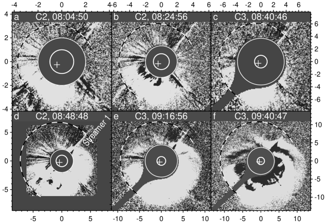
Figure 5.: The wave associated with CME1 in LASCO-C2 and C3 running-difference ratio images resized to compensate for the expansion of the wave front. The dashed oval outlines the outermost traces of wave 1. The circles denote the solar limb and the inner boundaries of the fields of view of the coronagraphs. The cross denotes the initial wave center. The axes show hereafter distances from the solar disk center in solar radii.

Figure 6 shows LASCO-C2 and C3 images of the main CME1 body (solid outline) resized according to the height-time plot in Figure 4a. The dashed oval outlines wave 1 (same as in Figure 5). The structure of CME1 is not identical in C2 and C3 images partly due to internal motions in the CME and partly due to its changing visibility in the course of expansion. The shape of the outlining oval is not obvious. Different eccentricities of the ovals do not significantly change the orientation of CME1 estimated in Section 5.3; the shape shown here is acceptable. Irrespective of the shape of the oval, the heading structure of expanding CME1 remained south from the ecliptic plane. Thus, its encounter with the Earth was unlikely (the solar disk center corresponds to the Sun – Earth line). CME1 was able to produce, at most, a glancing blow on the Earth’s magnetosphere.

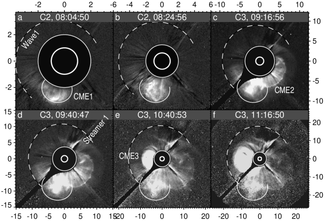
Figure 6.: CME1 in LASCO-C2 and C3 fixed-base ratio images resized to compensate for the expansion of the CME. The solid white open oval outlines the outer boundary of CME1. The dashed oval outlines the traces of wave 1 (same as in Figure 5). The circles denote the solar limb and the inner boundaries of the fields of view of the coronagraphs.

This analysis confirms the conclusion of Paper I that the CME1 onset was associated with the missed M1.2 flare at 07:29 in the east part of AR 10501 and contrary to the idea of KumarManoUddin2011 about its association with episode E2 at 07:41. Thus, eruption E2 was a confined one. Nevertheless, this sharp impulsive eruption produced a shock wave.

4.2 Shock 1 Produced by Confined Eruption at 07:41

Figure 7 presents traces of a shock wave propagating near the solar surface in wide-band GOES/SXI images and SOHO/EIT 195 Å images produced with a lower imaging rate. The SXI_spectrum.mpg movie in the electronic version of the paper shows the shock traces in GOES/SXI images (upper right corner) along with the dynamic radio spectrum. The outline of the shock front in the figure and the movie was calculated by using Equation (8) for propagation of a shock front along the spherical solar surface with homogeneous distribution of plasma parameters (the ellipses are intersections of the spheroidal wave front with the spherical solar surface). We used $t_{0}=$ 07:41:00 and $\delta=2.55$. The wave epicenter (slanted cross) is fixed at slightly ahead of the visible edge of the ejection at $t_{0}$ (see Paper I). Traces of the expanding wave front are distinct in later EIT images in the southeast to southwest directions. Most likely, a fixed south brightening denoted ‘SB’ in Figure 7e was due to eruption of CME1.

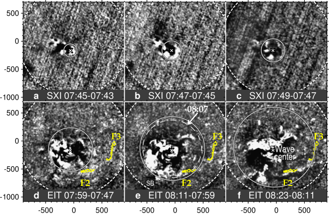
Figure 7.: Near-surface traces of shock 1 in GOES/SXI and SOHO/EIT 195 Å running difference-ratio images. The solid ellipses calculated with $\delta=2.55$, $t_{0}=$ 07:41:00 outline the expanding shock front. The dashed ellipse in panel (e) corresponds to 08:07. The yellow contours outline filaments F2 and F3. The large dashed circles denote the solar limb.

The near-surface portion of the shock front was distorted at a large-scale inhomogeneity above the long filament channel traced by filaments F2 and F3 (yellow in Figures 7d – 7f). The shock front entered this enhanced-density region above filament F2 at about 08:07. The filament started to ‘wink’ sequentially appearing and disappearing in the red and blue wings of the H$\alpha$ line. Figure 8 shows variations of the average brightness of the whole filament F2 relative to its close environment (photometry was made by an automated method).

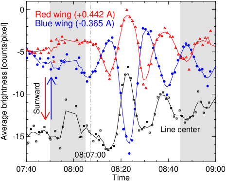
Figure 8.: Oscillations of filament F2 observed in the H$\alpha$ line center (black) and the red and blue wings (KSO). The symbols present the measurements. The curves show them smoothed over three neighbors. The shading marks the intervals of cloudy weather. The arrows indicate the changes of brightness corresponding to the sunward direction of the filament motion. The vertical broken line marks a probable onset time (08:07) of the anti-phase oscillations.

Distinct anti-phase oscillations in the blue and red wings started at about 08:07 (dash-dotted line) from the downward motion of the filament pushed by the tilted shock front. The oscillations with a period of 16 min probably reflect a self oscillation mode of the whole filament but might be affected by a wave trail and arrival of the second shock (discussed later) at about 08:15. A separate analysis of the east, middle, and west portions of filament F2 showed that all the three parts oscillated in-phase with each other.

The fastest motion of the filament occurred at 08:23 in an upwards direction, when it was darker in the blue wing than in the line center. This indicates that its Doppler shift was larger than the mid point between the blue wing and line center ($\approx 10$ km s^-1). On the other hand, the absence of an overturn in the blue-wing light curve in phase with the red wing near the valley at 08:23 suggests that the Doppler shift did not exceed the blue mid-wing wavelength ($\approx 20$ km s^-1). Thus, the highest line-of-sight velocity of the filament was $V_{\mathrm{LOS}}\approx 15$ km s^-1 (cf. Tripathi2009).

The dynamic spectrum in Figure 9c composed from the Culgoora (until 08:00), Learmonth, and San Vito data shows a harmonic band-split type II burst. Its parameters are typical of type II bursts associated with shock waves propagating upward in the corona. The estimated shock speed was from 405 to 478 km s^-1.

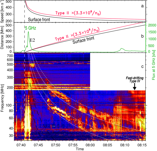
Figure 9.: Kinematics of shock 1 (a,b) in comparison with the microwave burst E2 (green, b) and shock manifestations in the dynamic spectrum of the first type II burst (c). The vertical dashed line marks the shock onset time $t_{0}=$ 07:41:00. The two pairs of white curves outline the split bands with the same $t_{0}$ and $\delta=2.60$. The black curves after 08:07 outline the N-like shift of the bands. The steep black dashed curves outline possible signatures of a quasi-parallel shock.

The outline for both pairs of the split bands was calculated as described in Section 2.2 with $\delta=2.60$ and the onset time $t_{0}=$ 07:41:00 (dashed vertical line), the same as for the near-surface shock traces. The plots for the velocities and distances vs. time are shown in Figures 9b and 9c. Due to the model dependence of estimates from radio spectra, the plots for the type II tracer (red) are uncertain by a factor of $3.3\times 10^{8}/n_{0}$, where $n_{0}$ is the actual plasma density at a characteristic distance $h_{0}\approx 100$ Mm. Near-surface shock propagation and kinematics of the source of the type II burst closely correspond to each other.

Comparison with near-surface shock traces in Figure 7 shows that the type II burst started when the shock front was located somewhere above regions 10501, 10503, and the bifurcation region. While the outline matches the overall evolution of the drift rate, both actual bands deviate from the outline like an inclined ‘S’ by 07:54. The band splitting disappears by 08:00. These properties disagree with a usual interpretation of band spitting due to emissions from the downstream and the upstream regions, implying instead emissions of split bands from two extended coronal structures located close to each other Grechnev et al. (2011a). The S-like deviation of the split bands and their merger afterwards suggests that the shock front encountered a high closed structure deflected by the shock.

At 08:07 the type II’s bands underwent an N-like shift to higher frequencies (black solid outline), suggesting that the shock front entered an enhanced-density region. Figure 7e and ‘winking’ filament F2 confirm that this really occurred at that time. These facts along with the properties of the band splitting indicate that the type II emission was most likely generated in a nearly radial structure stressed by a quasi-perpendicular shock (shock normal relative to the magnetic field). On the other hand, fast-drifting features at about 07:42 – 07:45, which were possibly harmonically related, hint at a possible much faster quasi-parallel shock passage. The black dashed curves outline possible harmonics.

A sketch in Figure 10 outlines our model of a coronal wave excited in an active region (AR). The positions of the wave front in the corona at three consecutive times $t_{1}$, $t_{2}$, and $t_{3}$ are denoted by the dotted curves, and their corresponding near-surface traces are shown with the solid ellipses. The arrow $\mathbf{grad}\,V_{\mathrm{fast}}$ represents the conditions in the low corona above the active region favoring the wave amplification and formation of a discontinuity at $t_{1}$. The blast-like wave is expelled from the AR core into regions of weaker magnetic fields. The shock front crossing the current sheet inside a coronal streamer excites a type II burst.

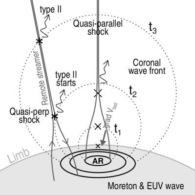
Figure 10.: Fast MHD shock wave excited by an impulsive eruption in an active region (AR) and the appearance of type II emissions excited by the quasi-perpendicular shock in a remote streamer and by the quasi-parallel shock in the streamer above AR. The slanted crosses denote the rising wave center at three consecutive times $t_{1}$, $t_{2}$, and $t_{3}$.

A wide-band type IV burst, which appeared after 08:11 at 180 MHz and relatively rapidly drifted to lower frequencies, will be discussed in Section 4.4.

4.3 CME2 at 08:49 and Shock 2

To find a possible relationship between the expansion of CME2 and radio signatures of the associated shock wave, the shock onset time should be estimated. The highest accuracy of the estimation can be achieved from the analysis of the radio spectrum in Figure 11c, which was composed from the Learmonth and San Vito data (its low-frequency part below 35 MHz is suppressed due to interference).

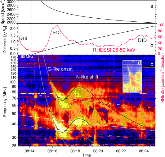
Figure 11.: Kinematics of shock 2 (a,b) and its manifestations in the dynamic spectrum of the second type II burst (c). The red curve in panel (b) is the RHESSI HXR flux. The inset (d) shows screen dump of the type II onset in raw Learmonth file displayed by a standard viewer. The almost vertical thin dotted line outlines the type III burst. The nearly horizontal lines trace extensions of the first type II burst. The remaining paired curves outline different harmonic components of the second type II burst with $t_{0}=$ 08:14:12 (vertical dashed line).

The drift rate of the type II burst was atypically high and started, in fact, from infinity. Its sharp C-like onset at about 08:15:35, also visible in the inset (d), suggests a flatwise encounter of the shock front with a nearly radial structure (see Grechnev2011_I). Just after this encounter, the contact region between the shock front and the streamer-like structure bifurcated, and one emission source moved up, while another one moved down thus producing the C-like feature.

Then both type II bands broadened considerably and underwent an N-like shift to higher frequencies, while the initial bands possibly continued. This behavior can be due to a portion of the shock front entering into a denser region similar to the corresponding feature of the first type II burst. The body of the second type II was crossed by the bands of the first type II burst, whose drift rate was much slower. They are outlined in Figure 11c with a pair of dashed lines and a white line (its corresponding fundamental band was below 25 MHz at that time).

A probable onset time of the shock wave estimated from the drift of the second type II burst falls within a valley between peaks E4B and E4C in Figure 11b. The valley is due to overlap of the decay of peak E4B and rise of peak E4C in the total HXR emission. A probable onset time of peak E4C is marked by a type III burst at 08:14:35 (crossed by the first type II). Type III bursts are considered as prompt indicators of non-thermal processes. By referring to this type III burst and extrapolating its drift to its probable highest frequency of 2 GHz, we estimate the shock 2 onset time $t_{0}=$ 08:14:12, which reconciles all its considered manifestations. The drift of the type II burst can be fit with an uncertainty of $t_{0}$ as large as $\pm 30$ s, while a considerably wider uncertainty is allowable to fit expansion of the outer halo component of CME2.

To outline the complex features of the type II burst, we adopt the hypothesis of the shock front entering into a denser region. The initial bands outlined with the black-on-white curves correspond to $\delta=2.65$. The black dotted curves outlining the high-frequency boundaries of the broadened bands were calculated with a considerably flatter density falloff $\delta=2.1$. The outline of the N-like feature was calculated by assuming a wide Gaussian-shaped density enhancement in the way of the shock wave. The complex structure of the type II burst and insufficient quality of the dynamic spectrum does not allow us to understand the behavior of the bands after 08:20.

The outer non-structured halo of CME2 outlined with the white oval in Figure 12 resembles traces of wave 1 in Figure 5. The shock-wave regime of the halo is supported by the type II burst and features discussed later. We therefore call the outer component ‘shock 2’ and the inner one ‘CME2’. Most likely, the eruption site of CME2 and source of shock 2 were within a region limited by AR 10501, 10503, dimming D2, and bifurcation region Rb (Figure 3d) rather close to the solar disk center, which we adopt for simplicity as the origin of the plots.

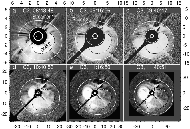
Figure 12.: Traces of shock 2 in resized LASCO-C2 and C3 running-ratio images. The circles denote the solar limb and the inner boundaries of the fields of view of the coronagraphs. The large white oval outlines the outermost halo envelope of CME2. The dashed oval outlines the outermost envelope of the arcade-like inner CME2 component (same as in Figure 14).

The green kinematical plot in Figure 13a calculated by using Equation (8) with the onset time of $t_{0}=$ 08:14:12 found from the dynamic spectrum agrees with the measurements in the CME catalog of the fastest feature related to CME2 (symbols). The white ovals outlining the halo envelope of CME2 in Figure 12 (see also the CME2.mpg movie) correspond to this curve. Deviations of streamer 1 ahead of shock 2 (which make shock 2 visible) are due to preceding wave 1. The structure poleward from streamer 1 makes visible the streamer belt deflected by shock 2. Concavity of the halo above the north pole region is expected for a shock wave (Section 5.1). These facts, as well as the high speed (green in Figure 13b), strongly support the shock-wave nature of the halo ahead of the main CME2 body (the dashed oval).

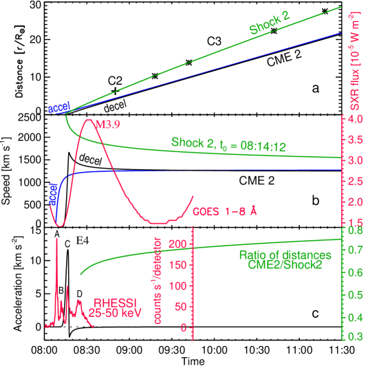
Figure 13.: Measurements of CME expansion for both the wave (green) and arcade-like components (blue accelerating, black decelerating). (a) Height-time plot. The green curve fits the shock wave. The symbols represent the measurements from the CME catalog. (b) Velocity-time plots in comparison with the GOES 1 – 8 Å light curve (red). (c) Acceleration of the CME along with the HXR time profile (red) and the ratio of distances CME2 to shock 2 (green).

To coordinate expansion of the halo with the second type II burst, we adjust the density model to bring the distances ($2.2R_{\odot}$) and speeds (2000 km s^-1) of the halo and the type II source into coincidence at 08:25 (the ending time of Figure 11). In fact, this assumption means a spherical shock front propagating in an isotropic medium. Even with this idealization, the difference between the speeds over the plotted parts in Figures 11a and 13b does not exceed 20%. The corresponding reference density $n_{0}=6.4\times 10^{8}$ cm^-3 is close to the Saito model (see Grechnev2011_I). Figures 11a and 11b show the initial parts of the kinematical plots for the shock 2 front calculated with this density model. Comparison of the dynamic spectrum with the distance–time plot in Figure 11b and images in Figure 7 shows that the type II burst started at a distance of $\approx 0.4R_{\odot}$ (08:15:35) from the source region roughly corresponding to the position of filament F2, and the N-like deviation started at $\approx 0.7R_{\odot}$ (08:16:50) roughly corresponding to filament F3. The somewhat larger distance and the gradual shape of the N-like deviation of type II-2 suggest a larger height of its source relative to type II-1. This assumption is consistent with the absence of the initial parts of the bands in type II-2, which were split in type II-1; shock 2 probably developed above the structure, from which these bands of type II-1 were emitted.

The inner arcade-like component of CME2 had a pronounced spine outlined in Figure 14 with the solid white oval. The dashed oval outlines the outermost envelope of the inner component including the intrusion region. Both ovals match the expanding CME2. The height-time plot used in compensating its expansion and plotting the ovals is shown in Figure 13a.

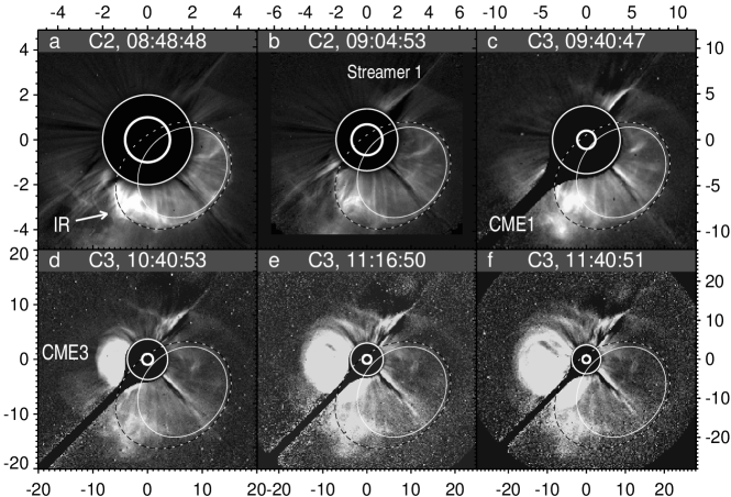
Figure 14.: CME2 in LASCO-C2 and C3 fixed-base ratio images resized to compensate expansion of the CME. The white oval outlines the spine of the main arcade-like structure. The dashed oval outlines the outermost envelope of the arcade-like structure. The circles denote the solar limb and the inner boundaries of the fields of view of the coronagraphs.

Expansion of CME2 was nearly self-similar with minor deviations. To keep the arcade spine within the white ovals, we slightly change their parameters with time. Figures 14a – 14f reveal a progressive displacement of the white oval southwest from the solar disk center, i.e., from the Sun – Earth line. The main leading part of CME2 is not expected to encounter the Earth. On the other hand, the wide outermost part outlined with the dashed oval increasingly covered the solar disk. These properties of CME2 indicate that its arcade-like part was directed southwest from the Earth and, most likely, could only produce a glancing blow on the Earth’s magnetosphere. The intrusion region remained south of the Earth.

Gopal2005 estimated the onset time for the inner CME2 component as $\approx$ 08:20 and its small acceleration. However, our measurements outlining the whole CME2 show that its expansion speed in the LASCO field of view was constant. LASCO images do not allow us to understand whether CME2 accelerated or decelerated. We compared plots for both kinematical types with X-ray light curves. The latest possible onset time achievable for accelerating kinematics corresponds to the blue curves in Figures 13a and 13b; later onset times produce infinite results in Equations (4) and (7). The velocity starts to rise too early with respect to the red SXR GOES plot. In this case it is difficult to reconcile the velocity plots for the CME, shock, and the type II burst.

By contrast, the decelerating type of kinematics (black curves) provides acceptable results. The CME velocity in Figure 13b starts to rise simultaneously with the SXR emission. The decelerating self-similar part of the velocity plot shows reasonable correspondence with the green shock wave plot. A difficulty here is due to the fact that self-similar kinematics does not describe the initial stage of rising acceleration. We have described the impulsive acceleration stage with a Gaussian profile (as we did in Paper I; see also Grechnev2011_I), combined the increasing velocity with the decreasing self-similar one, and computed the distance and acceleration from the combined velocity. The resultant impulsive acceleration up to $\approx 12$ km s^-2 almost coincides with the HXR peak E4C, the deceleration peak of about $-1.5$ km s^-2 marks the onset of the self-similar stage, and then acceleration decreases by the absolute value. Kinematical plots with similar shapes and parameters have been previously presented by Temmer et al. (2008; 2010) and Grechnev et al. (2008; 2011a).

The green curve in Figure 13c presents the ratio of distances CME2 to shock 2 from the eruption site (right $y$-axis). The relative distance monotonically decreased for two reasons. Firstly, CME2 moved nearly earthward, while the halo corresponded to the lateral shock front, whose expansion was not facilitated by a trailing piston. Thus, the lateral and especially rear shock was closer to a freely propagating blast wave. Secondly, even the shock front ahead of the CME2 tip decelerated and eventually must transform to a pure bow shock.

4.4 Overall Dynamic Radio Spectrum and an Extra Ejection

Figure 15 presents an overall picture of the whole event including microwave and hard X-ray bursts E1 – E4 (same as in Figures 2c and 2d) and a dynamic radio spectrum composed as a mosaic from pieces provided by several observatories in different frequency ranges and time intervals. The combined spectrum uses data from the Culgoora Solar Observatory (18 – 1800 MHz) until 08:00 (b and c), Learmonth and San Vito stations at 25 – 180 MHz (c), three parts form Bleien Observatory (180 – 2000 MHz) at 08:00 – 08:43 (b), a set of fixed-frequency records from San Vito to fill the gaps in panel (b), and the Wind/WAVES spectrum from the RAD2 receiver at 1 – 14 MHz.

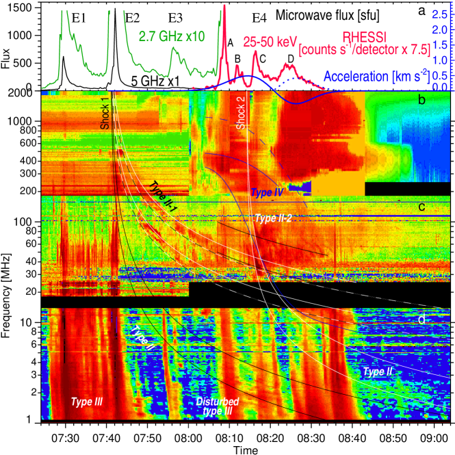
Figure 15.: Microwave (black and green) and HXR (red) time profiles (a) and an overall dynamic spectrum composed as a mosaic from observations of several instruments at decimeter, meter (b, c), and decameter (d, Wind/WAVES) wavelengths. The solid black, white, and dashed black-white curves outline the type II bursts (same as in Figures 9 and 11). The blue curves outline the fast-drifting type IV burst. The leading blue low-frequency envelope of the type IV burst was calculated from the acceleration presented with the blue curve in panel (a). The dashed part of the acceleration plot shows the absolute value of deceleration. The left $y$-axis in panel (a) quantifies the microwave and HXR fluxes (see Figures 2c and d). The right $y$-axis quantifies the acceleration.

The black and white curves of different line styles outline signatures of the two shock waves discussed in the preceding sections. The fast-drifting feature suggesting a quasi-parallel shock 1 has a pronounced continuation at decameters after 07:48 (the first pair of black lines) visible initially as a wide green band and later traced by disturbed type III bursts during 08:13 – 08:22 (see, e.g., Pohjolainen2008). The second type II burst also continues at decameters as a wide green band between 1.5 and 3.5 MHz during 08:40 – 08:58 with earlier indication of drifting features between the pair of the white curves. Relating this drifting burst to interaction between two CMEs proposed by KumarManoUddin2011 is not justified: this was a normal shock-associated type II burst. The type II emission at decameters is presumably produced by the shock front crossing a wide portion of the streamer belt with a relatively wide range of densities that determines its wide frequency band.

The gap between the Wind/WAVES spectrum and ground-based observations hinders identification of the harmonic number for the type II emissions at decameters. They are outlined assuming the dominant fundamental emission, although a stronger harmonic emission might be expected due to its weaker absorption. The alternative outline is possible but requires a density falloff of $\delta\approx 2.9$, which seems to be too steep at moderate latitudes. Such an outline coordinated with the metric type II burst produces a slightly higher drift rate at decameters than the observed one. CaneErickson2005 showed that the fundamental emission at decameters sometimes dominates, which possibly justifies our outline. Thus, we reproduce the drift rate of the decametric type IIs, while identification of their harmonic structure remains an open question.

Groups of type III bursts (especially clearly visible at decameters) provide further support to our identification of the eruptions. A dense type III group between 07:27 and 07:40 indicates the ongoing escape of non-thermal electrons into open magnetic structures probably associated with the CME1 liftoff, which started at E1. The situation is drastically different after confined eruption E2, when type IIIs rapidly terminate. Even the weak episode E3 produced a clear type III response. A series of type IIIs marks the fourfold event E4 suggesting a complex eruption, which has been partly studied in Paper I.

One more slowly drifting burst was reported as a type II by observers in Bleien to occur at 08:04 – 08:33. However, its evolution is opposite to the type IIs associated with shocks 1 and 2, and the bandwidth became quite broad. This burst is outlined with the blue curves in Figure 15. The solid curves outline the suggested fundamental band, and the dashed curve outlines a possible high-frequency envelope of the harmonic emission. The trailing edge of this burst is difficult to recognize and interpret.

The drift rate of this burst started from a near-zero value, which excludes its relation to a wave. The large bandwidth suggests that this was a type IV burst. It had an atypically high drift rate up to very low frequency (but not exceptional—see, e.g., Leblanc2000). Relation of this burst to the body of CME2 is unlikely due to the gradual acceleration up to the maximum speed during 08:04 – 08:14 implied by the drift rate, whereas CME2 sharply accelerated during E4C at about 08:16. Relating its drift rate to the Saito or Newkirk density model has not resulted in anything matching the observed CMEs.

There is a different option. The lowest frequency of a radio burst is determined by the plasma frequency $f_{\mathrm{P}}=9\times 10^{3}n^{1/2}$ in an emitting volume. Assuming the frequency drift to be due to the density decrease in an expanding spherical volume with radius $r$, $n\propto r^{-3}$, we have adjusted acceleration (blue in Figure 15a) to match the low-frequency envelope of the type IV burst. The initial density of $1.8\times 10^{9}$ cm^-3 corresponds to 380 MHz. The spatial scale is uncertain. With $r_{0}=30$ Mm corresponding to the bifurcation region Rb, the initial part of the type IV burst’s envelope corresponds to the expanding motion visible in GOES/SXI images in Figure 16 (see also the SXI_spectrum movie). Manifestations of the expansion are not expected to be observed later on, because the expanding feature moved away from the Sun. The velocity of the latter motion cannot be estimated from the radio spectrum.

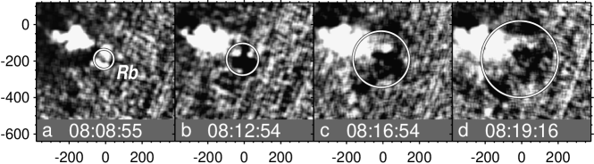
Figure 16.: Expansion visible in GOES/SXI running difference ratios probably corresponding to the type IV burst. The radius of the circle was calculated from acceleration in Figure 15a and exactly corresponds to the blue outline of the leading low-frequency envelope of the type IV burst in Figures 15b – 15d.

The radial expansion of the ejection responsible for the type IV burst accelerated up to $\approx 480$ m s^-2 at about 08:14:22 (the radial speed at that time was $V_{r}\approx 180$ km s^-1), reached a maximum speed $V_{r\,\max}\approx 300$ km s^-1, and then decelerated to $V_{r\,\mathrm{final}}\approx 100$ km s^-1. According to Paper IV (Grechnev et al., in preparation), the average Sun – Earth transit speed of the ICME responsible for the geomagnetic superstorm was $\overline{V}\approx 865$ km s^-1 (with an initial speed $V_{0}\gsim 930$ km s^-1). Thus, this ejection probably expanded within a narrow cone with an angle of $2V_{r\,\mathrm{final}}/\overline{V}<14^{\circ}$. Moving earthward almost exactly from the solar disk center and expanding within such a narrow cone, this ejection should appear in the LASCO-C2 field of view ($\geq 2R_{\odot}$) at a distance $>16R_{\odot}$ so that the Thomson-scattered light would be meager. According to the estimates in Paper I, the mass of this ejection should be $\ll 5\times 10^{15}$ g. The weak expansion and low mass have made this CME invisible for LASCO.

5 Discussion

5.1 Shock Waves

Analysis of the observations in the preceding section has revealed a complex chain of CMEs and waves. Table 2 summarizes the results. The most noticeable fact is that the confined eruption E2 undoubtedly produced a shock wave. Its presence is confirmed by the type II-1 burst, a detailed correspondence between its drift and structure with the observed near-surface propagation of the ‘EUV wave’, the ‘winking’ filament F2, and a possible decametric type II burst due to the quasi-parallel shock. All of these manifestations are quantitatively coordinated with each other by the power-law description (8) of an impulsively excited shock wave quasi-freely propagating like a decelerating blast wave.

Table 2.: CMEs and waves revealed in the event.

Time	Episode	CME	Wave
07:29	E1	CME1 onset	Wave 1
07:41	E2	No	Shock 1
08:14 – 08:16	E4C	CME2 onset	Shock 2
08:07 – 08:30	E4A – E4D	Invisible CME

Paper I has revealed that a portion of filament F1 was impulsively heated between 07:39:59 and 07:41:27. The apparent speed of this portion sharply reached $\approx 300$ km s^-1 in the plane of the sky, suggesting that its real speed along the filament leg was $\approx 770$ km s^-1 (at an angle of $\approx 23^{\circ}$), which most likely produced considerable pressure pulse. This was followed by an impulsive jet-like ejection with acceleration up to 2 km s^-2 and a maximum speed of 450 km s^-1 (both in the plane of the sky). Each of these two impulsive phenomena could have played a role of an impulsive piston; contributions from both are possible. When the shock wave started, the related M3.2 flare only began to gradually rise being unable to produce a significant pressure pulse to excite the shock (cf. Grechnev2011_I). Eruption E2 had not produced any CME which excludes the usually assumed bow-shock excitation by the outer CME surface. This event presents a convincing pure case of shock wave excitation by an impulsive eruption.

Similarly, shock 2 was excited during the early rise phase of the E4C HXR burst in association with the onset of CME2. The velocity and acceleration plots of CME2 (black in Figures 13b and 13c) demonstrate its impulsive-piston behavior, while the propagation of shock 2 had the same decelerating pattern as shock 1 (green in Figures 13a and 13b) described by Equation (8). The shock-wave nature of this disturbance is confirmed by the fast-drifting type II-2 burst traced up to decameters with its drift rate and uncommon structural features described by the same Equation (8), its super-Alfvénic speed, and the non-structured faint spheroidal halo in LASCO images (Figure 12) both ahead of the arcade-like CME2 and well behind its rear part. There are additional features expected for propagation of a shock wave.

Figure 17 compares the halo envelope of CME2 observed by LASCO-C3 with an expected distortion of the shock front in the presence of the heliospheric current sheet (HCS) calculated by Uralova1994. The red arrow in Figure 17a points at a coronal ray, which is a portion of the coronal streamer belt aligned along the line of sight. This orientation makes it distinctly visible. The streamer belt is the origin of the HCS.

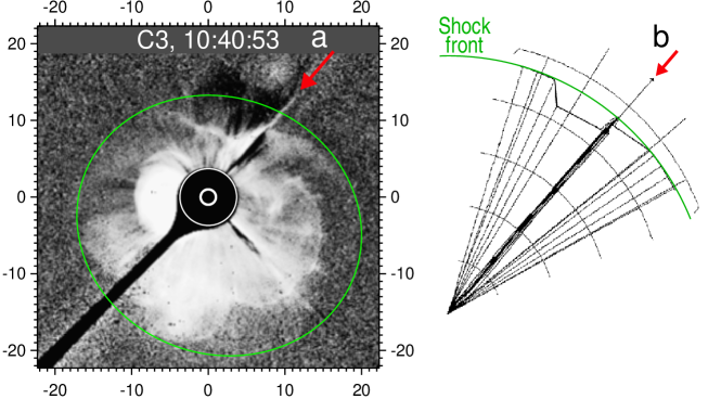
Figure 17.: Propagation of the shock front (green) along the streamer belt: (a) the outer halo envelope of CME2 observed by LASCO; (b) the calculated picture adopted from Uralova and Uralov (1994). The arrow points at the streamer.

Uralova1994 addressed the propagation of a fast-mode MHD shock wave along the HCS in the WKB approximation. Figure 17b presents Figure 5 of Uralova1994 rotated to correspond to the orientation in Figure 17a. The red arrow indicates the HCS inside a radially diverging slow wind flow of enhanced density bounded by the two long radial lines within $\pm 10^{\circ}$. A solar source of the shock wave was considered apart from the HCS base on the solar surface (not shown), which was located at the vertex of the ray trajectories. The thick polygonal chain is the calculated shock front far enough from the Sun (the polygonal shape was due to a limited number of rays in the calculations). Its outermost portions coincide with the green wave front calculated without the presence of the HCS. A portion of the front in the close vicinity of the HCS shown with the dashed arrow-like line represents the strongest shock. It is due to the effect of regular energy accumulation in the vicinity of the HCS. Uralova1994 first suggested that a small velocity component towards the HCS was able to initiate a magnetic reconnection process accompanying a shock wave.

Comparison of Figures 17a and 17b shows an overall qualitative similarity of distortions of the wave front in the vicinity of the HCS that cause its concave shape. Unlike the calculated picture, the real HCS in Figure 17a is not plane parallel to the line of sight. Its portion between the streamer under the arrow and the dip nearly above the north pole has been brought into view by the shock and corresponds to different distances and position angles.

Shock 2 developed 33 min after the slower shock 1 at nearly the same place in the plane of the sky and underwent the N-like shift of the bands about 10 min after shock 1. This approach indicates that the trailing shock 2 reached the leading shock 1 before its appearance from behind the occulting disk of LASCO-C2. The two shocks should combine into a single stronger one Grechnev et al. (2011a). Parameters of shock 2 have unlikely changed significantly, because shock 1 was much weaker. Due to probable coupling of the two shocks, manifestations of shock 1 in LASCO images are not expected.

Our knowledge of wave 1 and related CME1 is poorer relative to shocks 1 and 2. Its near-surface traces have not been detected, neither was there a type II burst. On the other hand, traces of wave 1 in LASCO images resembling a partial halo, the decelerating kinematics also described by Equation (8), and its rather high speed of $>850$ km s^-1 up to at least $10R_{\odot}$ indicate its shock-wave nature like shocks 1 and 2. The absence of a type II burst and an ‘EUV wave’ might be due to different propagation conditions with its relatively low speed.

The widely presumed scenario of bow-shock excitation by the outer surface of a CME is not confirmed. Ignition of a shock by a flare pressure pulse is also unlikely Grechnev et al. (2011a). This historically oldest scenario was based on an idea that the increase of the plasma beta in flare loops up to $\beta\approx 1$ could produce a significant disturbance. However, Grechnev2006 showed that the high-beta condition is a normal situation in a flare. The plasma pressure in flare loops increased due to chromospheric evaporation must be balanced by the dynamic pressure of reconnection outflow coming from above. Even with $\beta>1$, the net effect is an increase of all sizes of a flare loop as low as $\sqrt[4]{1+\beta}$, so that the expected disturbance should be too small to produce a shock.

The major conclusion of this section related to the 20 November superstorm is that the outer halo component of CME2 was most likely a trace of a quasi-freely propagating shock wave and did not indicate the earthwards direction of CME2.

5.2 Consequences for a Problem of “EIT Waves”

Our analysis in Section 4 touched the long-standing challenging wave-like disturbances observed in EUV, usually called “EIT waves” or “EUV waves”. Debates over the nature of these transients have lasted 15 years and do not appear to have terminated so far (see, e.g., Warmuth (2010; 2011) for a review). Their different nature from the Moreton waves was prompted by their different observed velocities and other properties seemingly inconsistent with those of fast-mode MHD shock waves. A basic solution was initially proposed by Warmuth2001 and then developed by these authors in several studies (e.g., Warmuth et al. 2004a; 2004b; 2005, and others). The idea is that both kinds of phenomena are due to propagation of decelerating fast-mode MHD shock waves. The Moreton waves are usually observed at shorter distances, where the wave speed is higher; EUV transients are observed at longer distances, where the speeds of decelerating waves are lower. Grechnev et al. (2011a; 2011b) demonstrated that at least two kinds of EUV transients visible as ‘EUV waves’ did exist and could be observed simultaneously. One kind of EUV transient is due to plasma compression on top of a developing CME and by its sides [basically consistent with the approach of Chen et al. (2002; 2005)]. Near-surface manifestations of such transients are of non-wave nature and remain not far from an eruption site. The second kind of EUV transient propagating over long distances is consistent with the initial interpretation of the Moreton waves as lower skirts of coronal waves proposed by Uchida1968. (Note in this respect the term ‘coronal counterpart of a Moreton wave’ used by some authors is confusing.) The apparent discrepancies between properties of propagating EUV transients and other shock signatures such as the Moreton waves, type II bursts, and outer CME halos thus have a simple explanation.

Grechnev2011_I showed that the most probable source of an MHD shock wave is an impulsive eruption of a developing magnetic flux rope. This is also consistent with the event in question. The ends of an eruptive flux rope are fixed, while the velocity of the eruption is highest in the direction of its expansion (often non-radial, but mostly at a large angle with the solar surface). Thus, an MHD disturbance excited by an impulsive eruption is anisotropic, and the speed of its near-surface propagation is considerably less than the upward one. For this reason, the near-surface propagation velocity of an EUV transient is typically much less than that of a type II source.

The fact that the Moreton waves are typically considerably faster than EUV transients suggests that the Moreton waves are manifested at stronger shocks than ‘EUV waves’. This circumstance is also clear: to produce a Moreton wave, a shock wave has to penetrate to relatively denser layers of the solar atmosphere that significantly weakens the shock. By contrast, EUV signatures of a shock are observed in higher coronal levels of lower density, so that deceleration and damping of a shock does not prevent its observation at much larger distances.

These circumstances show that reports on ‘winking filaments’ driven by ‘EIT waves’, which were slower than type II burst sources, do not contradict their excitation by shocks, as Tripathi2009 conjectured. A similar phenomenon considered in Section 4 present a confirmation. It should also be noted here that the oscillating filament on 4 November 1997 reported by Eto2002, which was sometimes considered as an argument against the shock-wave nature of ‘EIT waves’, dealt with an EUV transient poorly observed by EIT. By using the difference ratios $-0.01<I_{\mathrm{wave}}<0.01$ (see Section 2) of EIT images observed during this event, one can detect faint but clear signatures of a propagating disturbance at 06:13:54 at a much longer distance from the eruption site than the authors found — almost near a coronal hole at the north pole.

5.3 Orientations of the CMEs

To confirm and elaborate our preliminary conclusions about the orientations of CME1 and CME2, now we try to employ a model which allows one to estimate three-dimensional (3-D) geometric and kinematical parameters of a CME observed by LASCO coronagraphs in the plane of the sky. The so-called ice-cream cone model initially proposed by FisherMunro1984 considers a CME as a cone with a vertex in the Sun’s center. This model underwent several elaborations. We use the model described by XueWangDou2005. The model allows one to estimate the radial velocity $|V|$ of a CME along its axis, the orientation of the axis with respect to the Earth, and the angular width $\alpha$ of the CME cone. For our purposes it is convenient to express the results provided by the model in an ecliptic longitude ($\lambda>0$ west of the earthward direction) and latitude ($\phi>0$ north of the earthward direction).

To use the model of XueWangDou2005, an experimental dependence is evaluated of the plane-of-sky velocity $V_{\mathrm{m}}(\psi)$ of the CME envelope in LASCO images on the azimuthal position angle $\psi$. Then a set of parameters determining the orientation and axial speed of the CME is optimized by using the least-squares fit of the measured set $V_{\mathrm{m}}(\psi)$ to a calculated dependence $V_{\mathrm{c}}(\psi)$ (by minimizing the standard deviation $\sigma$). To expedite adjustment of parameters in the optimization process, we employed a genetic algorithm Mitchell (1999). Constraints on the fitting parameters should be applied for implementation of this algorithm. We used the following constraints: $1000\leq|V|\leq 2000$ km s^-1, $10^{\circ}\leq\alpha\leq 70^{\circ}$, and $\lambda$ and $\phi$ within $\pm 40^{\circ}$ relative to the axis passing from the Sun’s center through the CME source region.

3-D parameters of CME1 and CME2 were estimated from eight sets of images observed with LASCO-C2 and C3. The contours of both main and wide envelopes of CME2 in Figure 14 are well defined with small uncertainties. This is not the case for CME1; estimations of its 3-D parameters were additionally complicated by a narrower range of position angles (see Figure 6) which CME1 occupied, being far from the halo geometry. Therefore, extra attempts were required to obtain better results for CME1. In these attempts, we had to adjust velocity constraints for each iteration by monitoring $\sigma$. Overall, the estimated parameters were reasonably stable while input measurements were varied within the limited ranges. The final results are listed in Table 3. The corresponding sketch of the ice-cream cones of CME1 and CME2 is shown in Figure 18 with different viewing directions.

Table 3.: Spatial parameters of CMEs estimated from the ice-cream cone model.

CME	Time	Longitude∗	Latitude∗	Span∗	Speed $|V|^{*}$	Deviation
No.	interval	$\lambda\ [^{\circ}]$	$\phi\ [^{\circ}]$	$\alpha\ [^{\circ}]$	[km s${}^{-1}]$	$\sigma$ [km s-1]
1	08:05–11:41	$-8\pm 0.7$	$-26\pm 1.8$	$28\pm 2.0$	$1950\pm 24$	8.1–13.5
2 Main	08:49–12:17	$17\pm 1.4$	$-16\pm 1.2$	$50\pm 2.4$	$1778\pm 9$	1.0–1.8
2 Wide	08:49–12:17	$13\pm 1.4$	$-18\pm 1.7$	$66\pm 2.5$	$1718\pm 55$	3.2–4.9

^∗Average and range of estimates from different images in the interval specified in column 2.

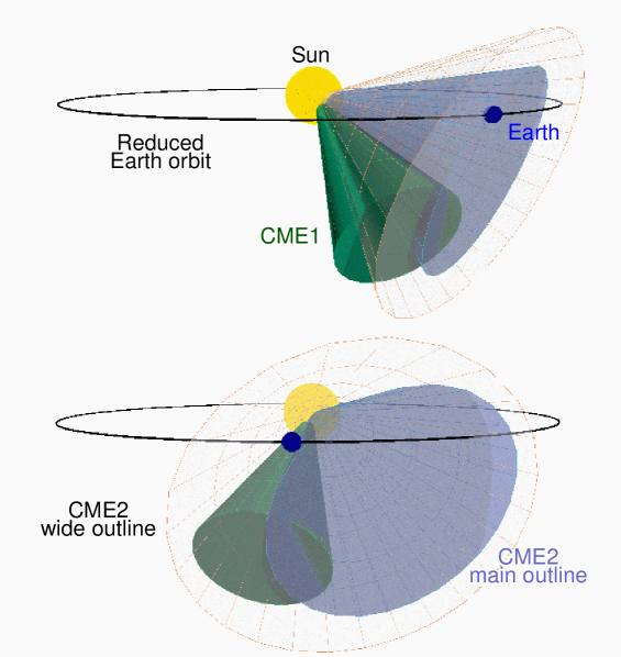
Figure 18.: Orientations of CME1 and CME2 estimated by means of the ice-cream cone model. The top and bottom panels represent different viewing directions.

Table 3 and Figure 18 confirm our preliminary conclusion that both CME1 and CME2 were not directed exactly earthwards. Each of the CMEs propagated mainly southward from the ecliptic plane, being only able to produce a glancing blow on the Earth’s magnetosphere. Ongoing expansion of an ICME suggests that the magnetic fields at its flanks were significantly weaker than at its nose. Due to magnetic flux conservation, the magnetic field strength at a fixed position of a self-similarly expanding ICME is inversely proportional to its instantaneous size squared (and the speed decreases linearly). For example, if an ICME flank hits the Earth at a distance of $1/\sqrt{2}$ of the heliocentric distance of the ICME nose, then the magnetic field at the flank should be reduced by a factor of 2 with respect to the central encounter. To our knowledge, the total magnetic field strength $|\mathbf{B}|\approx 56$ nT in the 20 November 2003 magnetic cloud was close to a record one. Still stronger fields were only observed in November 2001: on 6th, $|\mathbf{B}|\approx 66$ nT, and on 24th, $|\mathbf{B}|\approx 57$ nT (A. Belov, 2012, private communication). If the encounter of the 20 November 2003 MC with the Earth were a non-central encounter, one would have observed significantly stronger magnetic field; which is unlikely.

Thus, direct responsibility for the superstorm of magnetic structures of CME1 or CME2 appears to be doubtful. On the other hand, the mutual lateral pressure of CME1 and CME2 should considerably affect their expansion as well as any structures between them including the hypothetical invisible CME. This circumstance hints at possible causes of its weak expansion.

5.4 Eruption near the Solar Disk Center

Now we have sufficient information to assume what could have occurred near the solar disk center between 08:07 and 08:17. Paper I has established that the eruptive filament F1, which lifted off at an angle of $\approx 60^{\circ}$ to the solar surface, at about 08:07 collided with a topological discontinuity and bifurcated. The major mass of the filament moved nearly along the solar surface afterwards and had not left the Sun. At the same time and place, a nearly spherical structure developed and erupted with an initial speed of motion away from the Sun of $\gsim 930$ km s^-1. Its very slow expansion almost exactly from the solar disk center (the established radial expansion speed of $\approx 100$ km s^-1) and the earthward orientation have made it invisible for the LASCO coronagraphs. The only reasonable cause of its development was the anomalous collision of the eruptive filament F1 with a magnetic obstacle.

Most likely, one more product of this collision was the development of the coreless arcade-like CME2. Magnetic fields in a pre-eruption arcade are nearly potential (rot$\mathbf{B}\approx 0$), and therefore the arcade was unlikely to erupt by itself. Thus, CME2 was probably forced to erupt being hit from below. Its onset time of about 08:15 indicates that its probable cause was also the eruptive filament F1, whose active role was established in Paper I. This assumption is supported by decelerating kinematics of CME2 (see Figure 13b). The observations lead therefore to the following picture. The magnetic flux rope developed from filament F1 and moved southwest with an initial angle of $\approx 60^{\circ}$ to the solar surface ($\approx 23^{\circ}$ to the line of sight). When passing through the topological discontinuity near the solar disk center at a height of $\approx 100$ Mm, the eruptive filament (flux rope) caused an expansion of the arcade above it (in a normal case, the arcade would be a CME frontal structure), but failed to become its core. Instead, the filament disintegrated into two parts, one of which remained on the Sun, and the other one erupted as a ‘core’ (invisible CME), but apart from CME2. The initial velocity of the invisible CME $\gsim 930$ km s^-1 is comparable with the initial speed of CME2 ($\approx 1700$ km s^-1), confirming their association and the assumption that the eruption of CME2 was forced by the eruptive filament F1. Development of shock 2 at 08:14:12 was most likely related to this violent episode.

Separation of CME2 into the ‘coreless CME’ and ‘CMEless core’ (without the frontal structure) hints at a more complex relation between the CME parts than traditionally assumed. The core might be an active CME component responsible for its initiation and initial propagation, and the frontal structure might be a passive envelope arcade whose expansion is driven from inside. Note that the appearance of CME3 in Figure 3c supports this assumption: its core was pronouncedly twisted suggesting active motions followed by a kink instability, while the outer structures of CME3 consisted of steadily expanding closed long loops rooted on the Sun. After relaxation of the core, the whole CME expanded self-similarly. The difference between the loops in the structures of CME2 and CME3 was due to their orientations. Unlike CME2, in which the planes of the arcade loops were close to the line of sight, the planes of the frontal loops of CME3 were close to the plane of the sky.

The joint analysis of the dynamic radio spectrum and GOES/SXI images has shown that HXR peak E4D (the last one whose association was not revealed) corresponds to deceleration of the invisible CME. As discussed in Paper I, considerations and results of several researchers converge to the conclusion that HXR and microwave bursts presented a flare manifestation of magnetic reconnection responsible for acceleration of a developing flux rope, when the propelling toroidal force developed. Similarly, the deceleration reflected by the HXR peak E4D might be a response to another reconnection process. This process possibly destroyed magnetic structures providing the toroidal force so that only retarding magnetic tension responsible for deceleration persisted, and then the eruption probably disconnected completely, thus entering a free expansion stage. This speculation implies that HXR and microwave bursts indicate both acceleration and deceleration of CMEs, and that the self-similar expansion began, when the flare bursts ceased.

6 Conclusions

Our detailed analysis of the complex solar eruptive event carried out in this paper and Paper I has led to a number of results, which are not only important in pursuing causes of the 20 November 2003 geomagnetic superstorm, but also are promising for better general understanding of solar eruptions, CMEs, related shock waves, and their various manifestations. In particular, identification of an outer halo CME component with a shock trace promises better estimates of orientation and velocity of CMEs and higher accuracy in predicting the arrival time of a corresponding ICME.

The shock waves revealed in this event provide further support for the concept of early impulsive-piston shock excitation by an eruptive structure proposed by Grechnev2011_I. A shock wave excited by a confined eruption at 07:41 presents a notable example confirming this scenario. On the other hand, the widely presumed bow-shock excitation scenario at the outer surface of a CME is not confirmed. Ignition of a shock by a flare pressure pulse is also unlikely.

Magnetic structures of neither CME1 nor CME2 appear to be appropriate candidates for the sources of the superstorm for the following reasons.

• CME1 erupted, most likely, at about 07:29 from the east part of AR 10501, where the helicity was excessively negative. CME1 was not earth-directed.

• The outer halo of CME2 was probably due to a spheroidal shock front and did not indicate the earthward direction of magnetic structures of CME2.

• Expansion of CME1 and CME2 close to each other probably caused their mutual compression, but there were no signs of reconnection between their magnetic structures.

• CME1 and CME2 were directed southward from the ecliptic plane, oblique with respect to the Sun – Earth line, being only able to produce a glancing blow on the Earth’s magnetosphere with a reduced geomagnetic effect.

These circumstances disfavor the idea of Chandra2010 about a positive-helicity eruption from AR 10501. The suggestions of KumarManoUddin2011 and Marubashi2012 related to the causes of the 20 November 2003 superstorm lose their basis. On the other hand, GOES/SXI and radio observations provide further support to the presumed additional CME which erupted close to the solar disk center. Its estimated characteristics confirm the assumption made in Paper I that its weak expansion within a narrow cone of $<14^{\circ}$ could make it invisible for LASCO and preserve its very strong magnetic field due to magnetic flux conservation.

Our study demonstrates that even a case study of a single event can supply rich information about solar eruptions, associated phenomena, and their consequences. The major condition of success was a combined analysis of multi-spectral data. It has been recognized that significant suggestions and milestones are provided by bursts generated by accelerated electrons. They are observed as flare bursts in hard and soft X-rays and microwaves as well as drifting radio bursts at longer radio waves. Our results emphasize particularly the following.

• Type III bursts are well-known signatures of non-thermal electrons. Their appearance can be indicative of acceleration processes occurring during eruptive episodes. In particular, our event demonstrated dense trains of type III bursts accompanying the CME lift-off.

• The concept of predominant excitation of type II bursts by decelerating quasi-perpendicular shocks in remote streamers allowed us to reconcile their various features with other signatures of propagating shock waves. In particular, this concept accounts for the delay of the type II onset time relative to HXR and microwave flare bursts and the relatively low starting frequencies of type II bursts. The latter becomes clear if one considers the tilted shock front excited at a height of $\approx 100$ Mm to encounter a remote streamer at some distance from the eruption site.

• The type IV burst discussed here was possibly a moving type IV, but we cannot confirm this possibility due to the absence of meter-wave imaging observations. The approach used here promises diagnostics of developing CMEs from type IV bursts with relatively fast drift.

In summary, the combined analysis of the multi-spectral observations carried out in Paper I and this paper makes it possible to construct a consistent picture of several observational facts and suggestions, some of which seemed to have been questionable. The outlined scenario accounts for most of these circumstances. Unanswered questions still remain, however. It is unclear what occurred in the magnetic structures of the eruptive filament in the bifurcation region, how the ‘CMEless core’ was formed, and how to reconcile the right-handed magnetic cloud with the left-handed pre-eruption structure. These issues will be addressed in Paper III. One more question is specifically what kind of structure reached the Earth on November 20 and produced the superstorm. This will be a subject of Paper IV.

Acknowledgements

We thank Viktoria Kurt for the CORONAS-F/SONG data, L. Kashapova and S. Kalashnikov for the assistance in data processing, and I. Kuzmenko for useful discussions. We are grateful to an anonymous reviewer for useful remarks. We thank the instrumental teams of the Kanzelhöhe Solar Observatory; MDI, EIT, and LASCO on SOHO (ESA & NASA project); the USAF RSTN Radio Solar Telescope Network; RHESSI; and the GOES satellites for the data used here. We thank the team maintaining the CME Catalog at the CDAW Data Center by NASA and the Catholic University of America in cooperation with the Naval Research Laboratory. This study was supported by the Russian Foundation of Basic Research under grants 11-02-00757, 11-02-01079, 12-02-00008, 12-02-92692, and 12-02-00037, The Ministry of education and science of Russian Federation, projects 8407 and 14.518.11.7047. The research was also partly supported by the European Commission’s Seventh Framework Programme (FP7/2007-2013) under the grant agreement eHeroes (project No. 284461), www.eheroes.eu.

References

- Brueckner et al. (1995) Brueckner, G.E., Howard, R.A., Koomen, M.J., Korendyke, C.M., Michels, D.J., Moses, J.D., et al.: 1995, Sol. Phys. 162, 357.
- Cane and Erickson (2005) Cane, H.V., Erickson, W.C.: 2005, ApJ 623, 1180.
- Cerrato et al. (2012) Cerrato, Y., Saiz, E., Cid, C., Gonzalez, W. D., Palacios, J.: 2012, J. Atmos. Solar-Terr. Phys. 80, 111.
- Chandra et al. (2010) Chandra R., Pariat, E., Schmieder, B., Mandrini, C.H., Uddin, W.: 2010, Sol. Phys. 261, 127.
- Chen (1989) Chen, J.: 1989, ApJ 338, 453.
- Chen (1996) Chen, J.: 1996, J. Geophys. Res. 1012, 27499.
- Chen et al. (2002) Chen, P. F., Wu, S. T., Shibata, K., Fang, C.: 2002, ApJ 572, L99.
- Chen, Fang, and Shibata (2005) Chen, P. F., Fang, C., Shibata, K.: 2005, ApJ 622, 1202.
- Chertok and Grechnev (2005) Chertok, I. M., Grechnev, V. V.: 2005, Astron. Reports 49, 155.
- Cremades and Bothmer (2004) Cremades, H., Bothmer, V.: 2004, A&A 422, 307.
- Delaboudinière et al. (1995) Delaboudinière, J.-P., Artzner, G. E., Brunaud, J., Gabriel, A. H., Hochedez, J. F., Millier, F., et al.: 1995, Sol. Phys. 162, 291.
- Eto et al. (2002) Eto, S., Isobe, H., Narukage, N., Asai, A., Morimoto, T., Thompson, B., et al.: 2002, PASJ 54, 481.
- Fisher and Munro (1984) Fisher, R.R., Munro, R.H.: 1984, ApJ 280, 428.
- Gopalswamy et al. (2005) Gopalswamy, N., Yashiro, S., Michalek, G., Xie, H., Lepping, R. P., Howard, R. A.: 2005, Geophys. Res. Lett. 32, L12S09.
- Gopalswamy et al. (2009) Gopalswamy, N., Yashiro, S., Michalek, G., Stenborg, G., Vourlidas, A., Freeland, S., Howard, R.: 2009, Earth, Moon, Planets 104, 295.
- Grechnev et al. (2005) Grechnev, V.V., Chertok, I.M., Slemzin, V.A., Kuzin, S.V., Ignat’ev, A.P., Pertsov, A.A., Zhitnik, I.A., Delaboudinière, J.-P., Auchère, F.: 2005, J. Geophys. Res. 110, A09S07.
- Grechnev et al. (2006) Grechnev, V.V., Uralov, A.M., Zandanov, V.G., Rudenko, G.V., Borovik, V.N., Grigorieva, I.Y., et al.: 2006, PASJ 58, 55.
- Grechnev et al. (2008) Grechnev, V.V., Uralov, A.M., Slemzin, V.A., Chertok, I.M., Kuzmenko, I.V., Shibasaki, K.: 2008, Sol. Phys. 253, 263.
- Grechnev et al. (2011a) Grechnev, V.V., Uralov, A.M., Chertok, I.M., Kuzmenko, I.V., Afanasyev, A.N., Meshalkina, N.S., Kalashnikov, S.S., Kubo, Y.: 2011a, Sol. Phys. 273, 433.
- Grechnev et al. (2011b) Grechnev, V.V., Afanasyev, A.N., Uralov, A.M., Chertok, I.M., Eselevich, M.V., Eselevich, V.G., Rudenko, G.V., Kubo, Y.: 2011b, Sol. Phys. 273, 461.
- Grechnev et al. (2013) Grechnev, V.V., Uralov, A.M., Slemzin, V.A., Chertok, I.M., Filippov, B.P., Rudenko, G.V., Temmer, M.: 2013, Sol. Phys. in press. doi: 10.1007/s11207-013-0316-6.
- Howard et al. (1982) Howard, R.A., Michels, D.J., Sheeley, N.R., Jr., Koomen, M.J.: 1982, ApJ 263, L101.
- Illing (1984) Illing, R.M.E.: 1984, ApJ 280, 399.
- Ivanov, Romashets, and Kharshiladze (2006) Ivanov, K.G., Romashets, E.P., Kharshiladze, A.F.: 2006, Geomagn. Aeron. 46, 275.
- Krall, Chen, and Santoro (2000) Krall, J., Chen, J., Santoro, R.: 2000, ApJ 539, 964.
- Kumar, Manoharan, and Uddin (2011) Kumar, P., Manoharan, P.K., Uddin, W.: 2011, Sol. Phys. 271, 149.
- Leblanc et al. (2000) Leblanc, Y., Dulk, G.A., Vourlidas, A., Bougeret, J.-L.: 2000, J. Geophys. Res. 105, 18225.
- Low (1982) Low, B. C.: 1982, ApJ 254, 796.
- Maričić et al. (2004) Maričić, D., Vršnak, B., Stanger, A.L., Veronig, A.: 2004, Sol. Phys. 225, 337.
- Marubashi et al. (2012) Marubashi, K., Cho, K.-S., Kim, Y.-H., Park, Y.-D., Park, S.-H.: 2012, J. Geophys. Res. 117, A01101.
- Miklenic et al. (2007) Miklenic, C.H., Veronig, A.M., Vršnak, B., Hanslmeier, A.: 2007, A&A 461, 697.
- Miklenic, Veronig, and Vršnak (2009) Miklenic, C.H., Veronig, A.M., Vršnak, B.: 2009, A&A 499, 893.
- Mitchell (1999) Mitchell, M.: 1999. An Introduction to Genetic Algorithms The MIT Press. Cambridge, Massachusetts, 158.
- Möstl et al. (2008) Möstl, C., Miklenic, C., Farrugia, C. J., Temmer, M., Veronig, A., Galvin, A. B., Vršnak, B., Biernat, H. K.: 2008, Ann. Geophys. 26, 3139.
- Pomoell, Vainio, and Kissmann (2008) Pomoell, J., Vainio, R., Kissmann, R.: 2008, Sol. Phys. 253, 249.
- Pohjolainen, Hori, and Sakurai (2008) Pohjolainen, S., Hori, K., Sakurai, T.: 2008, Sol. Phys. 253, 291.
- Neupert (1968) Neupert, W. M.: 1968, ApJ 153, L59.
- Sheeley, Hakala, and Wang (2000) Sheeley, N.R., Jr., Hakala, W.N., Wang, Y.-M.: 2000, J. Geophys. Res. 105, A3, 5081.
- Temmer et al. (2008) Temmer, M., Veronig, A. M., Vršnak, Rybák, J., Gömöry, J., Stoiser, S., Maričić, D.: 2008, ApJ 673, L95.
- Temmer et al. (2010) Temmer M., Veronig A. M., Kontar E. P., Krucker S., Vršnak B., 2010, ApJ 712, 1410.
- Tripathi, Isobe, and Jain (2009) Tripathi, D., Isobe, H., Jain, R.: 2009, Space Sci. Rev. 149, 283.
- Uchida (1968) Uchida, Y.: 1968, Sol. Phys. 4, 30.
- Uralova and Uralov (1994) Uralova, S. V., Uralov, A. M.: 1994, Sol. Phys. 152, 457.
- Uralov, Grechnev, and Hudson (2005) Uralov, A. M., Grechnev, V. V., Hudson, H. S.: 2005, J. Geophys. Res. 110, A05104.
- Vourlidas et al. (2003) Vourlidas, A., Wu, S.T., Wang, A.H., Subramanian, P., Howard, R.A.: 2003, ApJ 598, 1392.
- Wang, Zhang, and Shen (2009) Wang, Y., Zhang, J., Shen, C.: 2009, J. Geophys. Res. 114, 10104.
- Warmuth (2010) Warmuth, A.: 2010, Adv. Space Res. 45, 527.
- Warmuth (2011) Warmuth, A.: 2011, Plasma Phys. Control. Fusion 53, 124023.
- Warmuth et al. (2001) Warmuth, A., Vršnak, B., Aurass, H., Hanslmeier, A.: 2001, ApJ 560, L105.
- Warmuth et al. (2004a) Warmuth, A., Vršnak, B., Magdalenić, J., Hanslmeier, A., Otruba, W.: 2004a, A&A 418, 1101.
- Warmuth et al. (2004b) Warmuth, A., Vršnak, B., Magdalenić, J., Hanslmeier, A., Otruba, W.: 2004b, A&A 418, 1117.
- Warmuth, Mann, and Aurass (2005) Warmuth, A., Mann, G., Aurass, H.: 2005, ApJ 626, L121.
- Xue, Wang, and Dou (2005) Xue, X.H., Wang, C.B., Dou, X.K.: 2005, J. Geophys. Res. 110, A08103.
- Yashiro et al. (2004) Yashiro, S., Gopalswamy, N., Michalek, G., St. Cyr, O. C., Plunkett, S. P., Rich, N. B., Howard, R. A.: 2004, J. Geophys. Res. 109, A07105.
- Yermolaev et al. (2005) Yermolaev Yu. I., Zelenyi, L. M., Zastenker, G. N., Petrukovich, A. A., Yermolaev, M. Yu., Nikolaeva, N. S., et al.: 2005, Geomagn. Aeron. 45, 681.
- Yurchyshyn, Hu, and Abramenko (2005) Yurchyshyn, V., Hu, Q., Abramenko, V.: 2005, Space Weather 3, S08C02.
- Zhang and Dere (2006) Zhang, J., Dere, K. P.: 2006, ApJ 649, 1100.
- Zhang et al. (2001) Zhang, J., Dere, K.P., Howard, R.A., Kundu, M.R., White, S.M.: 2001, ApJ 559, 452.