Separability and Dynamical Symmetry of Quantum Dots

Abstract

The separability and Runge-Lenz-type dynamical symmetry of the internal dynamics of certain two-electron Quantum Dots, found by Simonović et al. [1], is traced back to that of the perturbed Kepler problem. A large class of axially symmetric perturbing potentials which allow for separation in parabolic coordinates can easily be found. Apart of the 2:1 anisotropic harmonic trapping potential considered in [1], they include a constant electric field parallel to the magnetic field (Stark effect), the ring-shaped Hartmann potential, etc. The harmonic case is studied in detail.
KEY WORDS: Quantum Dots, Separability, Dynamical Symmetry, Perturbed Kepler problem, Anisotropic Oscillator

Annals of Physics 347, 94 – 116 (2013)
http://dx.doi.org/10.1016/j.aop.2013.11.004

1 Introduction

A two-electron quantum dot (QD) in a perpendicular magnetic field, described by the Hamiltonian,

$$H=\sum_{a=1}^{2}\left[\frac{1}{2M}\left({\bm{p}}_{a}-e{\bm{A}}_{a}\right)^{2}+U({\bm{r}}_{a})\right]-\frac{a}{|{\bm{r}}_{1}-{\bm{r}}_{2}|}\,,$$ (1.1)

where the confining potential is that of an axially symmetric oscillator Simon ; Simon2 ,

$$U({\bm{r}})=\frac{M}{2}\left[\omega_{0}^{2}\big{(}x^{2}+y^{2}\big{)}+\omega_{z}^{2}z^{2}\right],$$ (1.2)

may carry unexpected symmetries. Firstly, the system splits, consistently with Kohn’s theorem, into center-of-mass and relative motion and the former system carries a Newton-Hooke type symmetry Kohn ; ZHAGK . Secondly, for the particular values of the frequency ratios

$$\tau=\frac{\omega_{z}}{\sqrt{\omega_{0}^{2}+\omega_{L}^{2}}}=1,\,2,$$ (1.3)

where $\omega_{L}$ is the Larmor frequency , the relative motion becomes separable in suitable coordinates Simon , which hints at further symmetry. This paper is devoted to the study of the latter, and to generalizing them to other axi-symmetric trapping potentials.

Our first step is to trace back the problem to those results found earlier for a particle without a magnetic field, ${\bm{B}}=0$ Alhassid ; Blumel . Choosing the vector potential ${\bm{A}}={\scriptstyle{\frac{1}{2}}}B(-y,x,0)$ and introducing $\bm{R}=({\bm{r}}_{1}+{\bm{r}}_{2})/2$ and ${\bm{r}}={\bm{r}}_{1}-{\bm{r}}_{2}$, the system splits into center-of-mass and relative parts. Disregarding the first, we focus our attention at the relative motion. Following Simon , the relative Hamiltonian becomes, after suitable re-definition,

$$H\equiv H_{rel}=-\frac{1}{2M^{*}}\big{(}{\overrightarrow{\nabla}}_{\rho}-eiA_{\rho}\big{)}^{2}+\frac{M^{*}}{2}\Big{(}\omega_{0}^{2}(x^{2}+y^{2})+\omega_{z}^{2}z^{2}\Big{)}-\frac{a}{r},$$ (1.4)

where $M^{*}=M/2$ is the reduced mass and we used units where $\hbar=1$. Now putting

$${\bm{r}}\to R(t)\,{\bm{r}},\qquad R(t)=\left(\begin{array}[]{cc}\cos\omega_{L}\,t&\sin\omega_{L}\,t\\[4.0pt] -\sin\omega_{L}\,t&\cos\omega_{L}\,t\end{array}\right),\qquad\omega_{L}=\frac{eB}{2M^{*}}$$ (1.5)

eliminates the vector potential altogether and the Schrödinger equation of relative motion, $\big{[}i{\partial}_{t}-H_{rel}\big{]}\psi=0$, goes over into

$$\left[i\partial_{t}+\underbrace{\,\frac{\bigtriangleup}{2}+\frac{a}{r}\,}_{Kepler}-\underbrace{\frac{1}{2}(\omega_{0}^{2}+\omega_{L}^{2})\left(x^{2}+y^{2}\right)-\frac{1}{2}\omega_{z}^{2}z^{2}}_{axi-symmetric\;oscillator}\right]\psi=0,$$ (1.6)

where we also assumed that $M^{*}=1$.

The rotational trick (1.5) allowed us, hence, to convert the constant-magnetic-field problem into that of the Kepler potential perturbed by an axially symmetric oscillator Alhassid ; Blumel . In what follows, we only study the latter problem, since all results can be translated to the constant-magnetic context by applying (1.5) backwards. Note that in the original QD problem the electrons repel and thus $a\propto-e^{2}<0$; for completeness, we also consider here the attractive Kepler case $a>0$. Our analysis bears also strong similarities with that of ions in a Paul trap Blumel .

2 Classical separability

We first study the classical context, where “separability” refers to that of the Hamilton-Jacobi equation. According to the Robertson Theorem (Cordani (Sec. 8.1.3., p. 169), see also Benenti ), classical separability does imply, in our case, that of the Schrödinger equation 4. Restricting ourselves to natural orthogonal systems, i.e., such whose Hamiltonian is

$$H=\frac{1}{2}\sum_{k=1}^{n}g_{k}(x_{1},\ldots,x_{n})\,p_{k}^{2}+V(x_{1},\ldots,x_{n}),$$ (2.1)

the answer is given by :

Theorem 1 (Stäckel Cordani ).

An $n$-dimensional system with Hamiltonian (2.1) is separable if and only if there exists (i) an invertible $n\times n$ matrix and (ii) a column vector,

$$(i)\;\;\text{{{U}}}=\left(\begin{array}[]{ccccc}U_{11}&\dots&U_{1k}&\dots&U_{1n}\\ \vdots&\vdots&\vdots&\vdots&\vdots\\ U_{n1}&\dots&U_{nk}&\dots&U_{nn}\\ \end{array}\right)\qquad\hbox{and}\qquad(ii)\;\;\underline{w}=\left(\begin{array}[]{c}w_{1}\\ \vdots\\ w_{n}\end{array}\right),$$ (2.2)

called the Stäckel matrix and the Stäckel vector, respectively, whose $j$-th rows are functions of $x_{j}$ only, and such that

$$\sum_{j=1}^{n}g_{j}U_{jk}=\delta_{1k},\qquad\sum_{j=1}^{n}g_{j}w_{j}=V.$$ (2.3)

That the Stäckel conditions are necessary is proved in Ref. Cordani . Here we only show how to use them. Put

$$\underline{p}^{2}=\left(\begin{array}[]{c}p_{1}^{2}\\ \vdots\\ p_{n}^{2}\end{array}\right),\qquad\underline{\alpha}=\left(\begin{array}[]{c}\alpha_{1}\\ \vdots\\ \alpha_{n}\end{array}\right),$$ (2.4)

where the $\alpha_{i}$s are arbitrary constants, and define the column vector $\underline{K}$ composed of $n$ functions,

$$\underline{K}(x_{j},p_{k})=\text{{{U}}}^{-1}\Big{(}\frac{1}{2}\underline{p}^{2}+\underline{w}\Big{)}.$$ (2.5)

Note for further record that, owing to (2.3), the first of these functions is in fact the Hamiltonian. Then the Hamilton–Jacobi Equation can be viewed as the first row of the system of $n$ equations

$$\underline{K}(x_{j},p_{k})=\,\underline{\alpha}.$$ (2.6)

Inverting this relation, $\frac{1}{2}\underline{p}^{2}+\underline{w}=\text{{{U}}}\underline{\alpha},$ defines $p_{k}$ implicitly as a function of the $x_{k}$ and of the constants $\alpha_{1},\ldots,\alpha_{n}.$ Putting $\frac{\partial S_{k}}{\partial x_{k}}=p_{k},$ we see that $S=\sum_{k}S_{k},\;S_{k}=S_{k}(x_{k},\alpha_{1},\ldots,\alpha_{n})$ is a complete integral. $S$ is in fact a solution of the Hamilton–Jacobi Equation by construction, and one readily shows that $\det\left(\frac{\partial^{2}S}{\partial\alpha_{j}\partial x_{k}}\right)\neq 0$, cf. Cordani .

The $n$ functions $\underline{K}(x_{j},p_{k})$ are first integrals in involution; they are quadratic in the momenta and, in coordinates allowing for separation, they do not contain products of the momenta. Our problem is precisely to find such coordinate systems, and the Eisenhart Theorem Eisenhart (Cordani chapter 8) provides us with a constructive method for doing this.

Turning to our concrete problem here, let us first remind the reader that the unperturbed Kepler Hamiltonian,

$$H_{\mathrm{Kepler}}=\frac{1}{2}{\bm{p}}^{2}-\frac{a}{r},$$ (2.7)

is separable in four coordinate systems, namely in spherical, (semi)parabolic, elliptic and spheroconical ones Cordani .

Turning to the QD problem which is our main interest here, the relative Hamiltonian $H\equiv H_{rel}$ reads, after elimination of the magnetic field by switching to rotating coordinates, the Kepler problem perturbed by a harmonic (but not necessarily isotropic) oscillator,

$$H=H_{\mathrm{Kepler}}+V,\qquad V=V_{osc}=\frac{1}{2}\Big{(}\omega_{\rho}^{2}\rho^{2}+\omega_{z}^{2}z^{2}\Big{)},$$ (2.8)

where $\rho=\sqrt{x^{2}+y^{2}}$, $\omega_{\rho}=\sqrt{\omega_{L}^{2}+\omega_{0}^{2}}$ cf. (1.6), and inquire about the values of the parameters $\omega_{\rho}$ and $\omega_{z}$ that make $H$ separable in one or another of the four “good” coordinate systems mentioned above.

$\bullet$ In the spherical case things are simple and do not require any calculation, and we only mention it for pedagogical purposes. For $\omega_{\rho}=\omega_{z}=\omega$ the perturbation we added is itself isotropic and the Hamiltonian is plainly separable in spherical coordinates. For completeness and for further use, we record the Stäckel matrix and ector, respectively,

U $$= \left(\begin{array}[]{ccc}1&-\frac{1}{r^{2}}&0\\ 0&1&-\frac{1}{\sin^{2}\theta}\\ 0&0&1\end{array}\right)\quad\Rightarrow\quad\text{{{U}}}^{-1}=\left(\begin{array}[]{ccc}1&\frac{1}{r^{2}}&\;\frac{1}{r^{2}\sin^{2}\theta}\\ 0&1&\frac{1}{\sin^{2}\theta}\\ 0&0&1\end{array}\right),$$ (2.15)

$$\underline{w} = \left(\begin{array}[]{c}-\frac{a}{r}\\ 0\\ 0\end{array}\right)+\left(\begin{array}[]{c}\frac{\omega^{2}}{2}r^{2}\\ 0\\ 0\end{array}\right).$$ (2.22)

The three commuting conserved quantities in involution mentioned above are, therefore, (i) the Hamiltonian, (ii) the half of the square of the total angular momentum, $L^{2}/2$, and (iii) the half of the squared $z$-component of the angular momentum, $L_{z}^{2}/2$, associated with the rotational ${\rm O}(3)$ symmetry — generalizing the pure Kepler problem Cordani . Here we do not pursue this issue and merely plot some trajectories, see Fig. 1.

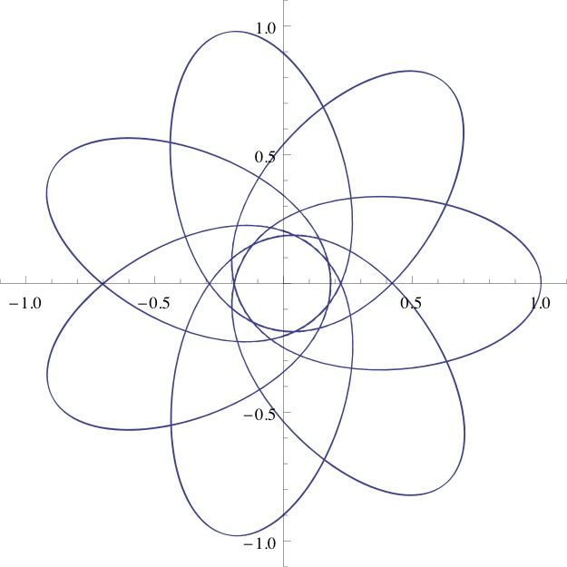
Figure 1: The Kepler problem combined with an isotropic oscillator is separable. The trajectories are perturbed Kepler ellipses rotating around in the plane perpendicular to the angular momentum.

$\bullet$ The (semi)parabolic case, which is our main concern in this paper, with coordinates $(\xi\geq 0,\eta\geq 0,2\pi\geq\varphi\geq 0)$,

$$x=\xi\eta\,\cos\varphi,\quad y=\xi\eta\,\sin\varphi,\quad z=\frac{1}{2}(\xi^{2}-\eta^{2}),$$ (2.23)

is non-trivial, though. The Stäckel matrix and vector read, respectively,

U $$= \left(\begin{array}[]{ccc}\xi^{2}&-1&-\frac{1}{\xi^{2}}\\ \eta^{2}&1&-\frac{1}{\eta^{2}}\\ 0&0&1\end{array}\right)\quad\Rightarrow\quad\text{{{U}}}^{-1}=\frac{1}{\xi^{2}+\eta^{2}}\left(\begin{array}[]{ccc}1&1&\;\frac{1}{\xi^{2}}+\frac{1}{\eta^{2}}\\ -\eta^{2}&\xi^{2}&\;\frac{\xi^{2}}{\eta^{2}}-\frac{\eta^{2}}{\xi^{2}}\\ 0&0&\;\xi^{2}+\eta^{2}\end{array}\right),$$ (2.30)

$$\underline{w} = \left(\begin{array}[]{c}-a\\ -a\\ 0\end{array}\right)+\left(\begin{array}[]{r}f(\xi)\\ g(\eta)\\ h(\varphi)\end{array}\right),$$ (2.37)

where $f(\xi)$ and $g(\eta)$ and $h(\varphi)$ are arbitrary functions. Assuming axial symmetry, $h(\varphi)=0$.

Then our clue is that for the perturbed Kepler problem (2.8) the Stäckel condition is satisfied when the first row in Eqns (2.5) holds, and this happens whenever the perturbing potential satisfies

$$(\xi^{2}+\eta^{2})V(\xi,\eta)=f(\xi)+g(\eta).$$ (2.38)

This simple but powerful separability condition will lead to large classes of separable potentials, see Sec. 5. For our anisotropic oscillator, it requires,

$$(\xi^{2}+\eta^{2})V_{osc}(\xi,\eta)=\frac{1}{2}\left(\frac{\omega_{z}}{2}\right)^{2}(\xi^{6}+\eta^{6})+\frac{1}{2}\left[\omega_{\rho}^{2}-\left(\frac{\omega_{z}}{2}\right)^{2}\right]\Big{(}\xi^{4}\eta^{2}+\xi^{2}\eta^{4}\Big{)}.$$

Separability is hence achieved when

$$\omega_{z}=2\omega_{\rho}\quad\hbox{i.e.,\; for}\quad\tau=2.$$ (2.39)

Those three commuting conserved quantities in (2.5) then read

$$H = \underbrace{\displaystyle\frac{1}{2(\xi^{2}+\eta^{2})}\left[p_{\xi}^{2}+p_{\eta}^{2}+\left(\frac{1}{\xi^{2}}+\frac{1}{\eta^{2}}\right)p_{\varphi}^{2}\right]-\frac{2a}{\xi^{2}+\eta^{2}}}_{Kepler\,Hamiltonian}\;+\;\underbrace{\frac{\omega_{\rho}^{2}}{2}\left(\xi^{4}-\xi^{2}\eta^{2}+\eta^{4}\right)}_{V_{osc}\;\;{with}\;\;\tau=2},\qquad$$ (2.40)

$$K_{z} = \displaystyle\frac{1}{2(\xi^{2}+\eta^{2})}\left[\xi^{2}p_{\eta}^{2}-\eta^{2}p_{\xi}^{2}+\left(\frac{\xi^{2}}{\eta^{2}}-\frac{\eta^{2}}{\xi^{2}}\right)p_{\varphi}^{2}\right]-a\,\frac{\xi^{2}-\eta^{2}}{\xi^{2}+\eta^{2}}-\frac{\omega_{\rho}^{2}}{2}\xi^{2}\eta^{2}(\xi^{2}-\eta^{2}),\qquad$$ (2.41)

$$L_{z}^{2}/2 = \frac{1}{2}p_{\varphi}^{2},$$ (2.42)

where $p_{\xi}=(\xi^{2}+\eta^{2})\,\dot{\xi},\,p_{\eta}=(\xi^{2}+\eta^{2})\,\dot{\eta}$. Translating into more familiar form,

$$H = \displaystyle\frac{{\bm{p}}^{2}}{2}-\frac{a}{r}+V_{osc},$$ (2.43)

$$K_{z} = \underbrace{({\bm{p}}\times{\bm{L}})_{z}\,-\,a\frac{z}{r}}_{Kepler\,Runge-Lenz}\;-\;\omega_{\rho}^{2}\,\rho^{2}z,$$ (2.44)

$$L_{z}^{2}/2 = \frac{1}{2}(\rho\dot{\varphi})^{2},$$ (2.45)

allows us to interpret these quantities : (i) $H$ is the perturbed Hamiltonian (2.8), as it should; (ii) $K_{z}$ generalizes the $z$ component of the Runge-Lenz vector and is indeed the separation constant found in Simon . The additional term $-\omega_{\rho}^{2}\rho^{2}z$ arises due to the perturbing oscillator potential. (iii) The third quantity is, once again, the half of the squared $z$ component of the angular momentum. The familiar Keplerian quantities Cordani and those of the $2:1$ anisotropic oscillator Makar ; Boyer are recovered when $V_{osc}=0$ or when the Kepler potential is switched off, $a=0$, respectively. Some classical trajectories will be presented in Sect. 3.

3 Reduction to and induction from the 2D problem

Returning to classical aspects, let us observe that the condition

$$L_{z}\equiv p_{\varphi}=0$$ (3.1)

constrains the motion into a “vertical” plane through the $z$ axis and in fact reduces the problem to the perturbed Kepler problem in 2D. Our strategy, in this Section, will be to work backwards, starting with the 2D case and then extending to 3D. Putting $\varphi=0$ (say) into the formulas in Section 2 provides us with two-dimensional ones. (2.23) yields, in particular, (semi)parabolic coordinates in the $x-z$ plane,

$$x=x_{+}=\xi\eta,\qquad z=\frac{1}{2}(\xi^{2}-\eta^{2}).$$ (3.2)

A subtlety arises, though: (3.2) is in fact only half of a coordinate system, since necessarily $x_{+}>0$, and should therefore be supplemented with $x_{-}=-\xi\eta$ to cover the whole vertical plane. This problem is not present in 3D, since the first coordinate is indeed $\rho>0$, and the angular variable $\varphi$ takes care of the $x<0$ half plane, namely for $\varphi=\pi$.

The 2D Stäckel matrices and resp. vector are simply those in (2.37) with the irrelevant $\varphi$-columns and rows erased. For our 2D anisotropic oscillator, separability is hence achieved for

$$\tau=\frac{\omega_{z}}{\omega_{\rho}}=2,$$ (3.3)

just like before in 3D, cf. (2.39). Our theory provides us now with $D=2$ conserved quantities in involution, namely with the separable 2D Hamiltonian,

$$H^{0}\equiv{H}\big{|}_{\varphi=0}=\underbrace{\frac{1}{2(\xi^{2}+\eta^{2})}\big{(}p_{\xi}^{2}+p_{\eta}^{2}\;-\;4a\big{)}}_{2D\ Kepler\ Hamiltonian}+\frac{\omega_{\rho}^{2}}{2(\xi^{2}+\eta^{2})}\big{(}\xi^{6}+\eta^{6}\big{)},$$ (3.4)

and with the Runge-Lenz-type conserved quantity

$$K_{z}^{0}\equiv K_{z}\big{|}_{\varphi=0}=\underbrace{\displaystyle\frac{1}{2(\xi^{2}+\eta^{2})}\left[\xi^{2}p_{\eta}^{2}-\eta^{2}p_{\xi}^{2}\right]-a\,\frac{\xi^{2}-\eta^{2}}{\xi^{2}+\eta^{2}}}_{2D\ Kepler\ Runge-Lenz-type}\;-\;{\omega_{\rho}^{2}}\underbrace{(\xi^{2}\eta^{2})(\frac{\xi^{2}-\eta^{2}}{2})}_{\rho^{2}z}\,.$$ (3.5)

cf. (2.41).

More symmetries

The unperturbed 2D Kepler problem has long been known to have an ${\rm O}(3)$ dynamical symmetry, generated by the two components of the Runge-Lenz vector, ${\bm{K}}=(K_{x},K_{z})$, and by the angular momentum, $L\equiv L_{y}$ perpendicular to the $x-z$ plane JauchHill ; CMI . In (semi)parabolic coordinates (3.2),

$$K_{x} = \frac{1}{\sqrt{-2E}}\Big{(}p_{\xi}p_{\eta}-2E\,\xi\eta\Big{)},$$ (3.6)

$$K_{z} = \frac{1}{\sqrt{-2E}}\Big{(}\frac{p_{\xi}^{2}-p_{\eta}^{2}}{2}-2E\,\frac{\xi^{2}-\eta^{2}}{2}\Big{)},$$ (3.7)

$$L = \frac{1}{2}\Big{(}\eta p_{\xi}-\xi p_{\eta}\Big{)},$$ (3.8)

where $E$ is a fixed value of the Kepler energy

$$H_{Kepler}=\frac{1}{2(\xi^{2}+\eta^{2})}\left(p_{\xi}^{2}+p_{\eta}^{2}\;-\;4a\right),$$ (3.9)

which is in fact the first term in (3.4), as anticipated. Putting $H_{Kepler}$ into (3.7) yields (3.5) with $\omega_{z}=0$. The expression (3.5) generalizes, hence, the $z$-component of the Runge-Lenz vector in the vertical plane, as anticipated.

Adding now, still in 2D, a perturbing oscillator potential to our pure Kepler problem destroys most of these symmetries. Most, but not all, though : the planar rotational symmetry generated by $L$ is plainly broken by the anisotropy, but, for $\tau=2$, the corrected version (3.5) of $K_{z}$ survives the perturbation. Numerical evidence also confirms that $K_{x}$ is also broken, except for $\tau=1/2$.

Further insight is gained by studying some classical trajectories. Our strategy is to start with the planar Kepler problem and then consider what happens when the relative strength of the perturbing oscillator, represented by $\omega_{\rho}$, is varied from weak to strong. The three rows of Figs. 2, 3 correspond to identical initial conditions, namely to

$$\left\{\begin{array}[]{llllll}x(0)=0,&z(0)=1,&\dot{x}(0)=1,&\dot{z}(0)=0,&&\hbox{{\color[rgb]{1,0,0}red}}\\ x(0)=1,&z(0)=0,&\dot{x}(0)=0,&\dot{z}(0)=1&&\hbox{{\color[rgb]{0,0,1}blue}}\\ x(0)=-\frac{1}{2},&z(0)=-\frac{1}{2},&\dot{x}(0)=-\frac{1}{2},&\dot{z}(0)=\frac{1}{2}&&\hbox{{\color[rgb]{.75,0,.25}purple}}\end{array}\right.\;,$$ (3.13)

with the pure Keplerian and oscillator cases indicated in dashed cyan and dotted magenta, respectively.

The same conventions is used later below for their 3D extensions in Figs. 4 and 5, where we start from a point on the 2D trajectory, but we add some non-trivial $y$-initial condition.

3.1 Attractive case $a>0$

We first consider the attractive Coulomb/Kepler interaction, $a>0$. As a result of the anisotropy [$\tau=2$] of the oscillator, the trajectories show a strong dependence on the initial conditions. Due to the complexity of the problem, we limit our investigations therefore to the particular case

$$|{\bm{x}}(0)|=1\qquad|\dot{{\bm{x}}}(0)|=1,$$ (3.14)

with the oscillator strength $\omega_{\rho}$ sweeping from small to big value, Hence $a=1$ and the initial Keplerian trajectory is the unit circle . Turning on the anisotropic oscillator manifestly squeezes the initial circle. For $\omega_{\rho}\to\infty$ the trajectories converge to those of pure $2:1$ anisotropic oscillator, indicated in dotted magenta.

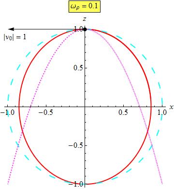
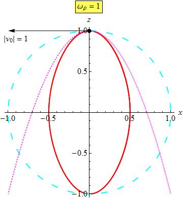
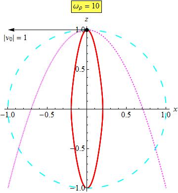
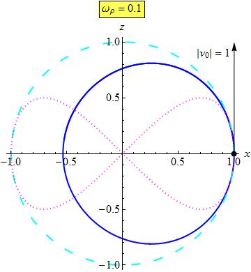
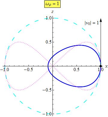
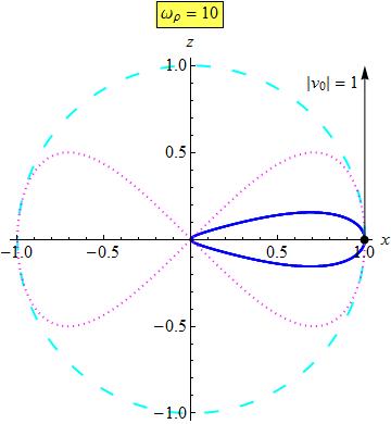
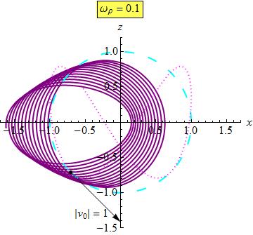
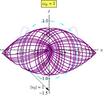
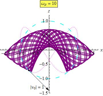
Figure 2: Trajectories in the classical planar Kepler problem perturbed with an axi-symmetric oscillator with anisotropy $\tau=\omega_{z}/\omega_{\rho}=2$. All figures have the same circular Keplerian limit but correspond to different initial conditions. For the “red” series the initial conditions correspond to the “North Pole” at the top of the Keplerian circle, and for the “blue” series they correspond to the “Far-East” one. The “purple” series has a “South-West” initial condition. Varying the strength of the perturbation from weak ($\omega_{\rho}=0.1$) through intermediate ($\omega_{\rho}=1$) to strong ($\omega_{\rho}=10$) deforms the trajectory from the pure Keplerian circle (dashed cyan) to the pure anisotropic oscillator (dotted magenta).

3.2 The repulsive case $a<0$

The Coulomb interaction between the electrons which constitute genuine Quantum Dots is repulsive, though : $a\propto-e^{2}<0$. In the pure Coulomb case, all trajectories are unbounded, namely hyperbolas. Switching on the harmonic trap converts the latter into bound ones, however. Intuitively, farther one goes stronger the harmonic force becomes, and ultimately wins against the weakening Coulomb repulsion. The only effect is that the Dot becomes somewhat larger.

A couple of trajectories are shown on Fig. 3. Here, all motions start from a point on the Keplerian hyperbola (in dashed cyan) with identical initial conditions as in the attractive case in Fig. 2 [as the colors suggest]. For $\omega_{\rho}\to\infty$ the trajectories tend to those of the pure anisotropic oscillator (in dotted magenta).

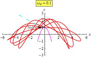
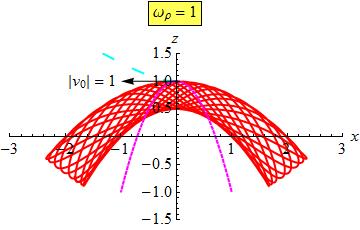
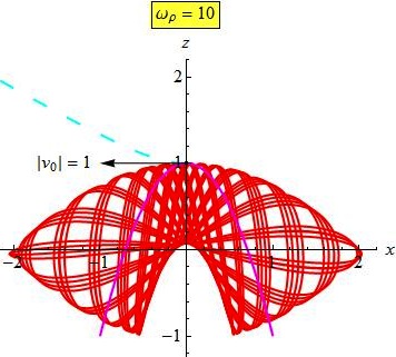
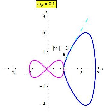
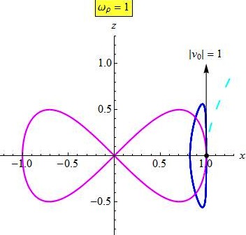
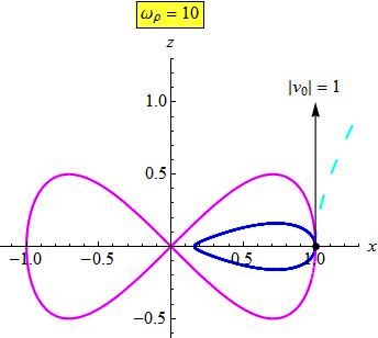
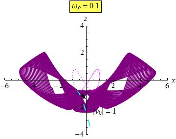
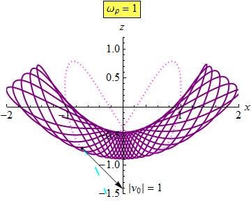
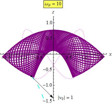
Figure 3: Trajectories for a repulsive Coulomb potential in the plane, perturbed with a $\tau=\omega_{z}/\omega_{\rho}=2$ anisotropic oscillator. Turning on the harmonic oscillator from weak ($\omega_{\rho}=0.1$) through intermediate ($\omega_{\rho}=1$) to strong ($\omega_{\rho}=10$) deforms the initial Keplerian hyperbola (in dashed cyan) into closed “potato” and ultimately into the dotted magenta “horizontal $8$” of the pure oscillator. All intial conditions are tangent to the Keplerian hyperbola, but in various positions. The “blue” series corresponds to the “Near-East” and the “red” series corresponds to the bottom of the Keplerian hyperbola. The “purple” series has a “South-West” initial condition.

3.3 Return to 3D

Relaxing the constraint $L_{z}\equiv p_{\varphi}=0$ in (3.1) plainly allows us to recover our 3D description. For the coordinates $(\xi,\eta,\varphi)$ separability guaranteed when $\tau=2$. (2.41) generalizes the planar conserved quantity $K_{z}$ in (3.5). Some trajectories are shown on Fig. 4, allowing us to check the conservation of $K_{z}$ also numerically.

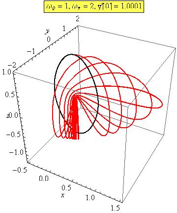
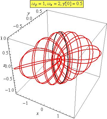
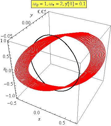
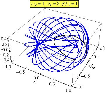
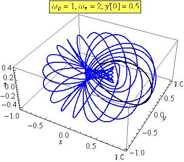
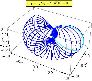
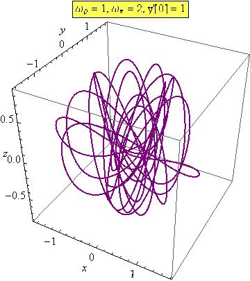
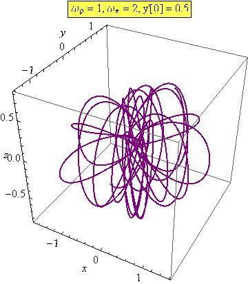
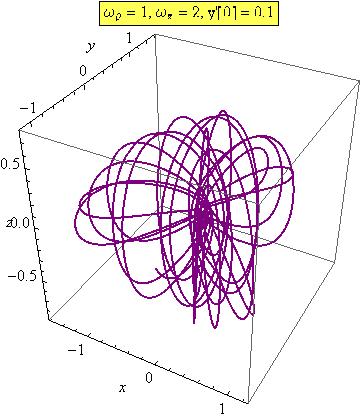
Figure 4: Some 3D trajectories in the perturbed Kepler problem with anisotropy $\tau=2$. As suggested by using the same colors, all figures have initial conditions lying on the 2D orbits of Fig. 2 with intermediate coupling $\omega_{\rho}=1$, but with non-vanishing initial $y$-velocities $\dot{y}(0)=1,\,0.5,\,0.1$. The initial 2D trajectories in the $x-z$ plane are indicated in black.

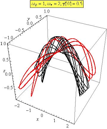
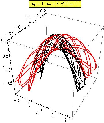
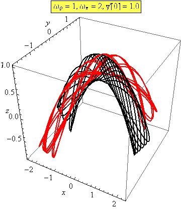
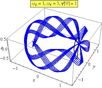
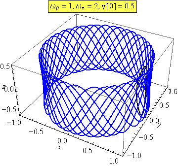
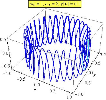
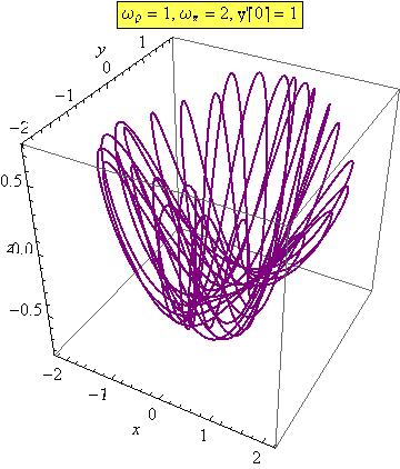
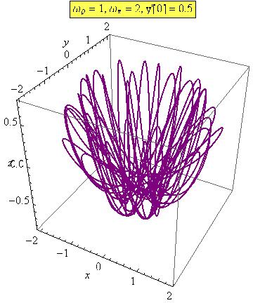
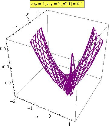
Figure 5: Some 3D trajectories in the repulsive Coulomb perturbed by a $\tau=2$ anisotropic oscillator. The initial 2D trajectories (in black) in the $x-z$ plane are only shown for the red series.

3.4 The curious $1/2$ case

It follows from our general theory that, in 3D, the values $\tau=1$ and $2$ are the only separable cases. Simonović et al. Simon observe, however, that, for $L_{z}=0$ states, the system is integrable also for $\tau=1/2$. See also Alhassid ; Blumel .

Let us explain how this comes about. [We again turn to classical mechanics]. Consider the Kepler+axially symmetric oscillator Hamiltonian in (2.40), and introduce new, “twisted” variables by rotating by $45$ degrees in $\xi-\eta$ space,

$$\mu=\frac{\xi+\eta}{\sqrt{2}},\qquad\nu=\frac{\xi-\eta}{\sqrt{2}},$$ (3.15)

completed with $\varphi$. Remarkably,

$$\begin{array}[]{lll}\xi\eta=\displaystyle\frac{\mu^{2}-\nu^{2}}{2}=\rho,&&\displaystyle\frac{\xi^{2}-\eta^{2}}{2}=\mu\nu=z,\\[6.0pt] \xi^{2}+\eta^{2}=\mu^{2}+\nu^{2}=2r,&&p_{\xi}^{2}+p_{\eta}^{2}=p_{\mu}^{2}+p_{\nu}^{2},\end{array}$$ (3.16)

i.e., the coordinate transformation $(\xi,\eta)\to(\mu,\nu)$ interchanges $\rho$ and $z$ while leaving $r$ and ${\bm{p}}^{2}$ invariant. Then it follows that, expressed in terms of the new coordinates $\mu$ and $\nu$, $H_{Kepler}$ will have the same form as (2.40) with the exception of the $p_{\varphi}^{2}$-term. The latter changes as

$$\frac{p_{\varphi}^{2}}{\rho^{2}}=\frac{p_{\varphi}^{2}}{\xi^{2}\eta^{2}}\quad\to\quad\frac{4p_{\varphi}^{2}}{(\mu^{2}-\nu^{2})^{2}}\,.$$ (3.17)

The equation is hence form-invariant only when this term is switched off by putting

$$L_{z}\equiv p_{\varphi}=0,$$ (3.18)

cf. (3.1). In other words, interchanging $\rho$ and $z$ is not a symmetry of the full 3-metric $d\rho^{2}+dz^{2}+\rho^{2}d\phi^{2}$ written in cylindrical coordinates, and hence not a symmetry of the full kinetic term in the free Hamiltonian ${\scriptstyle{\frac{1}{2}}}\big{(}p_{z}^{2}+p_{\rho}^{2}+{p_{\phi}^{2}}/{\rho^{2}}\big{)}$ unless $p_{\phi}=0$. Moreover, the exchange of $\rho$ and $z$ is not a global symmetry because $z$ ranges over all the reals while $\rho$ ranges only over the positive reals.

The oscillator potential $V_{osc}$ transforms in turn as

$$\frac{1}{2}\left[\omega_{\rho}^{2}\,\xi^{2}\eta^{2}+\big{(}\frac{\omega_{z}}{2}\big{)}^{2}(\xi^{2}-\eta^{2})^{2}\right]\;\to\;\frac{1}{2}\left[\big{(}\frac{\omega_{\rho}}{2}\big{)}^{2}\,\big{(}\mu^{2}-\nu^{2}\big{)}^{2}+\omega_{z}^{2}\,\mu^{2}\nu^{2}\right]\,,$$ (3.19)

which are of the same form as written with $\xi$ and $\eta$, up to interchanging the planar and vertical frequencies,

$$\omega_{\rho}\;\Longleftrightarrow\;\omega_{z}.$$ (3.20)

Hence, it is now the

$$\tau=\frac{\omega_{\rho}}{\omega_{z}}=\frac{1}{2}$$ (3.21)

case which is separable in the new coordinates — but only when the constraint (3.1) holds also.

We note that the $(\mu,\nu)$ in (3.15) can also be considered as coordinates in our vertical $(x-z)$ plane,

$$x=\frac{1}{2}(\mu^{2}-\nu^{2}),\qquad z=z_{+}=\mu^{2}\nu^{2},$$ (3.22)

This coordinate system suffers however of the same problems as $(\xi,\eta)$ in (3.2): while now $-\infty<x<\infty$ we necessarily have $z=z_{+}>0$ so that only the upper half-plane is covered, and (3.22) has to be supplemented with $z=z_{-}=-\mu^{2}\nu^{2}<0$.

Having understood these subtleties, $(\xi,\eta)\to(\mu,\nu)$ amounts of rotating the plane by $90^{{\,\raise 0.5pt\hbox{$\scriptstyle\circ$}\,}}$, $(x,z)\to(z,-x)$. In terms of (3.22), the Kepler+oscillator system is precisely (2.40) with the $p_{\varphi}$-term switched off and the frequencies interchanged as in (3.20). Our entire machinery can now be applied once over again, simply by trading $(\xi,\eta)$ for $(\mu,\nu)$. Separability is now obtained for

$$\tau=\frac{1}{2}.$$ (3.23)

The first line from the conserved quantities (2.5) is the Hamiltonian (3.4), up to changing the variables into $(\mu,\nu)$ and replacing $\omega_{z}$ with $\omega_{\rho}$. The second line yields in turn

$$\frac{1}{2(\mu^{2}+\nu^{2})}\left[-\nu^{2}p_{\mu}^{2}+\mu^{2}p_{\nu}^{2}\right]-a\frac{\mu^{2}-\nu^{2}}{\mu^{2}+\nu^{2}}-\frac{\omega_{\rho}^{2}}{4}\underbrace{(\mu^{2}\nu^{2})(\frac{\mu^{2}-\nu^{2}}{2})}_{z^{2}\rho}$$ (3.24)

which is also the same as $K_{z}^{0}$ in (3.5) after the interchange $(\xi,\eta)\leftrightarrow(\mu,\nu)$, as expected. Moreover, using ${p_{\mu}^{2}-p_{\nu}^{2}}=2p_{\xi}{}p_{\eta}$ (3.24) reduces, for $\omega_{\rho}=0$, to $-\big{(}-E/2\big{)}^{1/2}\,K_{x}$ in (3.6).

Note that the correction term in (3.24) which arises due to the $\tau=1/2$ oscillator is now $-(\omega_{\rho}/2)^{2}\,z^{2}\rho,$ as expected from the interchange $\rho\leftrightarrow z$, cf. (3.5).

Turning off the anisotropic oscillator restores the rotational and indeed the full ${\rm O}(3)$ symmetry, with the two components of the planar Runge-Lenz corresponding to separability in the two respective coordinate systems.

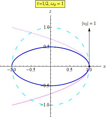
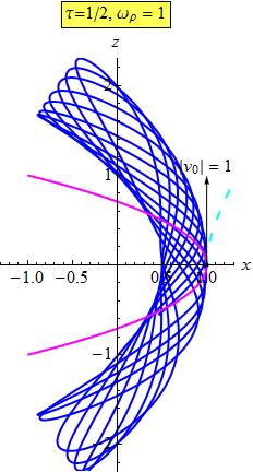
Figure 6: In the plane, the (i) [attrative] Kepler and the (ii) [repulsive] QD problem, perturbed by a $\tau=\omega_{z}/\omega_{\rho}=1/2$ oscillator is plainly separable in the twisted coordinates $(\mu,\nu)$, since the latter correspond to a rotation by $90^{{\,\raise 0.5pt\hbox{$\scriptstyle\circ$}\,}}$ degrees, interchanging the “long” and “short” directions and carrying $K_{z}$ into $-K_{x}$. The $\tau=1/2$-figure is indeed the rotated $\tau=2$-figure, in Figs. 2 and 3, respectively.

The regularity of the trajectories obtained for $\tau=1/2$ hints at an additional conserved quantity. So far, we derived such quantities from separability using the Stäckel approach. Separability is, however, not a necessary, only a sufficent condition for such a quantity, and we can, following Blümel et al. Blumel , proceed directly to search such a quantity. Their strategy is to observe, firstly, that the usual Keplerian Runge-Lenz vector is not conserved,

$$\dot{{\bm{K}}}_{Kepler}\neq 0\qquad\hbox{for}\qquad{\bm{K}}_{Kepler}={\bm{p}}\times{\bm{L}}\,-\,a\frac{{\bm{r}}}{r}\,.$$ (3.25)

If, however, $\dot{{\bm{K}}}_{Kepler}$ happens to be a total time derivative, $\dot{{\bm{K}}}_{Kepler}=\dot{d{\bm{C}}},$ then

$${\bm{K}}={\bm{K}}_{Kepler}-{\bm{C}}$$ (3.26)

will be conserved.

Let us first put $L_{z}=0$. For the combined Kepler + axisymmetric oscillator our condition requires, for the components written in cylindrical coordinates,

$$\left\{\begin{array}[]{cll}\omega_{\rho}^{2}\left(\displaystyle\frac{\tau^{2}-2}{2}z\dot{(\rho^{2})}+\dot{z}\rho^{2}\right)&=&\dot{C}_{z},\\[10.0pt] \omega_{\rho}^{2}\left(\displaystyle\frac{1-2\tau^{2}}{2}\rho\dot{(z^{2})}+\tau^{2}\dot{\rho}\,z^{2}\right)&=&\dot{C}_{\rho},\end{array}\right.$$ (3.27)

obtained by calculting $\dot{K}^{Kepler}$ using the eqns of motion,

$$\left\{\begin{array}[]{lllll}\ddot{\rho}-\displaystyle\frac{L_{z}^{2}}{\rho^{3}}&=&-\omega_{\rho}^{2}\rho&-&a\displaystyle\frac{\rho}{(\rho^{2}+z^{2})^{3/2}},\\[8.0pt] \ddot{z}&=&-\tau^{2}\omega_{\rho}^{2}z&-&a\displaystyle\frac{z}{(\rho^{2}+z^{2})^{3/2}}.\end{array}\right.$$ (3.28)

The conditions (3.27) require

$$\tau=2\;\Rightarrow\;C_{z}=\omega_{\rho}^{2}\rho^{2}z\qquad\hbox{or}\qquad\tau=\frac{1}{2}\;\Rightarrow\;C_{\rho}=\hbox{$\textstyle\frac{1}{4}$}\omega_{\rho}^{2}\rho z^{2},$$ (3.29)

which can not hold simultaneously, but provide us with either of our two previous cases,

$$\left\{\begin{array}[]{cllll}K_{z}^{0}&=&z\dot{\rho}^{2}-\dot{z}\rho\dot{\rho}-a\displaystyle\frac{z}{\sqrt{\rho^{2}+z^{2}}}-\omega_{\rho}^{2}\rho^{2}z&&\hbox{for}\quad\tau=2,\\[16.0pt] K_{\rho}^{0}&=&\rho\dot{z}^{2}-\dot{\rho}z\dot{z}-a\displaystyle\frac{\rho}{\sqrt{\rho^{2}+z^{2}}}-\hbox{$\textstyle\frac{1}{4}$}\omega_{\rho}^{2}\rho z^{2}&&\hbox{for}\quad\tau=1/2\end{array}\right.\quad.$$ (3.30)

Restoring 3D by lifting the constraint $L_{z}=0$ merely requires, in the separable case $\tau=2$, a further correction term,

$$K_{z}=K_{z}^{0}+\frac{z}{\rho^{2}}L_{z}^{2}\,,$$ (3.31)

which is indeed (2.41).

In the integrable but non-separable case $\tau=1/2$ Blümel et al. Blumel find the quartic conserved quantity

$$K^{(4)}=\big{(}K_{\rho}^{0}+\frac{L_{z}^{2}}{\rho}\big{)}^{2}+\big{(}K_{\varphi}^{0}\big{)}^{2}+\omega_{\rho}^{2}(\rho^{2}+z^{2})L_{z}^{2}\,,$$ (3.32)

where $K_{\rho}^{0}$ is the one in (3.30), and

$$K_{\varphi}^{0}=K_{\varphi}^{Kepler}=-\frac{\rho\dot{\rho}+z\dot{z}}{\rho}L_{z}\;.$$ (3.33)

$K^{(4)}$ is hence the [squared] length of the planar expression in (3.30), corrected with terms which involve $L_{z}\neq 0$. For $L_{z}=0$ (3.32) reduces to $K_{x}^{2}$, the square of $K_{x}$ in (3.6) and/or in (3.24). The conservation of (3.32) can be checked directly using the equations of motion.

It is now easy to understand the fundamental difference between the two semi-parabolic coordinates systems. The standard one we denoted by $(\xi,\eta)$ are naturally extended from 2D to 3D by adding $\varphi$, which unifies the two local 2D-charts associated with $x_{+}$ and $x_{-}$, since $\cos\pi=-1$ produces exactly the desired sign change.

For the “twisted coordinates $(\mu,\nu)$, however, the trick does not work: adding the polar angle $\varphi$ does not change $z>0$ into $z<0$, and so half of the space still remains uncovered.

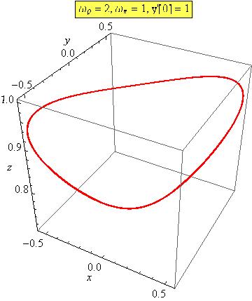
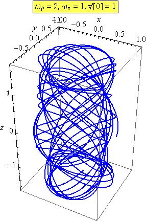
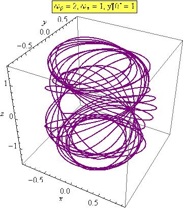
Figure 7: Trajectories in the integrable but non-separable case $\tau=\omega_{z}/\omega_{\rho}=1/2$ for various initial conditions.

4 The Quantum Picture

Let us now outline, for completeness, how things behave at the quantum level, cf. Refs. Simon ; Simon2 ; Alhassid . As it follows from our general theory, the only separable coordinate systems are the spherical one, for $\tau=\omega_{z}/\omega_{\rho}=1$, and the semi-parabolic one, for $\tau=\omega_{z}/\omega_{\rho}=2$. The first one of these is routine-like, and below we only study therefore the second case. The Schrödinger equation (1.6) for relative motion reads,

$$\left[i\partial_{t}+\underbrace{\,\frac{1}{2}\bigtriangleup+\frac{a}{r}\,}_{Kepler}-V_{osc}\right]\psi=0.$$ (4.1)

In semi-parabolic coordinates (2.23), the Laplacian is

$$\bigtriangleup=\frac{1}{\xi^{2}+\eta^{2}}\left[\frac{1}{\xi}{\partial}_{\xi}\big{(}\xi{\partial}_{\xi}\big{)}+\frac{1}{\eta}{\partial}_{\eta}\big{(}\eta{\partial}_{\eta}\big{)}+\left(\frac{1}{\xi^{2}}+\frac{1}{\eta^{2}}\right)\right].$$ (4.2)

Our task is hence to solve,

$$\left[2(\xi^{2}+\eta^{2})i\partial_{t}+\frac{1}{\xi}{\partial}_{\xi}\big{(}\xi{\partial}_{\xi}\big{)}+\frac{1}{\eta}{\partial}_{\eta}\big{(}\eta{\partial}_{\eta}\big{)}+\Big{(}\frac{1}{\xi^{2}}+\frac{1}{\eta^{2}}\Big{)}{\partial}_{\varphi}^{2}+2a-\omega_{\rho}^{2}\big{(}\xi^{6}+\eta^{6}\big{)}\right]\psi=0.$$ (4.3)

Then, consistently with the Robertson theorem Cordani , for $\tau=2$ i.e. for $\omega_{z}=2\omega_{\rho}$ the Ansatz

$$\psi(\xi,\eta,\varphi,t)=({\xi\eta})^{-1/2}u(\xi)v(\eta)e^{im\varphi}e^{-iEt}$$ (4.4)

separates the Schrödinger equation. Putting $\xi_{1}=\xi$ and $\xi_{2}=\eta$, we have,

$$\left[\frac{\,\,d^{2}}{d\xi_{i}^{2}}+2E\xi_{i}^{2}-\frac{m^{2}-\hbox{$\textstyle\frac{1}{4}$}}{\xi_{i}^{2}}+A_{i}-\omega_{\rho}^{2}\,\xi_{i}^{6}\right]u(\xi_{i}) = 0,\qquad i=1,2,$$ (4.5)

where the separation constants must satisfy the constraint

$$A_{1}+A_{2}=2a.$$ (4.6)

Note that (4.6) is indeed the only trace of the Kepler term. For a pure oscillator, $a=0$.

We now study (4.5) dropping the subscript $i=1,2$. Firstly, the $\xi^{-2}$ term can be eliminated, just like for Kepler, but putting $u=\xi^{(|m|+1/2)}U$, yielding,

$$\left[\frac{\,\,d^{2}}{d\xi^{2}}+2E\xi^{2}+A-\omega_{\rho}^{2}\,\xi^{6}\right]U(\xi)=0.$$ (4.7)

Regularity of $\psi$ at the origin is then guaranteed if $U$ and $V$ remain finite near the origin,

$$\psi(\xi,\eta,\varphi,t)\approx\rho^{|m|}U(\xi)V(\eta)e^{im\varphi}e^{-iEt}\qquad\xi,\eta\approx 0,$$ (4.8)

where we used $\xi\eta=\rho$. For large $\xi$ instead, the $6^{th}$-order oscillator term dominates. Dropping all other terms yields ${d^{2}U}/{d\xi^{2}}-\omega_{\rho}^{2}\,\xi^{6}\,U\;\approx\;0,$ whose approximate solution which vanishes at infinity is $U(\xi)\approx e^{-|\omega_{\rho}|\,\xi^{4}/4}$. For large $\xi$ and $\eta$ we have, hence, essentially a pure oscillator,

$$U(\xi,\eta)\approx e^{-|\omega_{\rho}|\,(\xi^{4}+\eta^{4})/4}=e^{-|\omega_{\rho}|\,(\rho^{2}+2z^{2})/2},\qquad\xi,\eta\to\infty.$$ (4.9)

More generally, our Eqn. (4.7) is, up to shifting the constraint (4.6) from $0$ to arbitrary constant $a$, identical to the one which describes the pure $2:1$ anisotropic oscillator in the plane Boyer .

For a detailed analytical study of Eqn. (4.7) the Reader is referred to the literature, and to Refs. Blumel ; Boyer ; Truong in particular. Some numerical solutions are plotted below.

We now turn to solving Eqns. (4.6)-(4.7) numerically for bound states. Let us observe that it is a two-parameter problem: the equation to be solved involves both the separation constant $A$ and the energy, $E$, which should be correlated.

For pure Kepler, or for the isotropic oscillator, the two separation constants can be unified into one. Then one can find the single “good” value which makes the solution bounded either analytically (namely from the poles of the hypergeometric function LandauLifshitz ), or also numerically.

Reduction to a one-parameter problem similar procedure would also work for the 2D pure oscillator with frequencies $\omega_{1}$ and $\omega_{2}$ in Cartesian coordinates, when can proceed as follows. The natural product Ansatz splits the Schrödinger equation into two 1D problems,

$$u_{i}^{\prime\prime}+[2\epsilon_{i}-\omega_{i}^{2}x_{i}^{2}]u_{i}=0,\quad\epsilon_{1}={\scriptstyle{\frac{1}{2}}}(E-C),\;\epsilon_{2}={\scriptstyle{\frac{1}{2}}}(E+C)\quad\Rightarrow\quad E=\epsilon_{1}+\epsilon_{2}.$$ (4.10)

The two eqns have identical [namely 1D oscillator] form, and are coupled through $E$ and $C$. But the two constants are, however, unified into single ones. Solving each of them independently for bound states yields the possible “good” values of the energies, namely $\epsilon_{i}=\omega_{i}(n_{i}+{\scriptstyle{\frac{1}{2}}})$. Then from (4.10) we infer the 2D spectrum,

$$E\equiv E_{n_{1},n_{2}}=\epsilon_{1}+\epsilon_{2}=\omega_{1}(n_{1}+{\scriptstyle{\frac{1}{2}}})+\omega_{2}(n_{2}+{\scriptstyle{\frac{1}{2}}}).$$ (4.11)

For our $2:1$ system, in particular, $\omega_{1}=2\omega_{2}\equiv 2\omega$, and the 2D energy becomes one with a single principal quantum number $N$,

$$E=E_{N}=\omega\,(N+\hbox{$\textstyle\frac{3}{2}$}),\qquad N=2n_{1}+n_{2}.$$ (4.12)

The energy levels are therefore $[N/2]+1$-times degenerate, as it follows from the formula for $N$. Keeping $N$ fixed also tells us which individual solutions should be paired together.

To solve the problem in parabolic coordinates, we would need a relation between $E$ and $A$ similar to the one above that we don’t have, though, let alone for the pure oscillator .

So far for the oscillator alone. But in the coupled oscillator + Kepler case, the problem is plainly not separable in Cartesian coordinates, and so we can not determine the exact energy spectrum separately, and a two-parameter search for bound states had to be developed, providing us with Fig. 8 and Table 1, as well as with Figs. 9, 10 and Table 2, respectively.

Fig. 8 shows the solutions obtained for the pure $2:1$ oscillator. The energy values and degeneracies found numerically are consistent with the exact results. This search can be viewed, therefore, as a test for our two-parameter search.

The results listed in Table 2 and illustrated on Figs. 9 and 10 show that turning on the Kepler interaction reduces the energy. This is clear from that for the attractive Kepler interaction $a>0$ (i) the energy is negative; moreover, (ii) The gravitational attraction it pulls closer the charges, reducing also the oscillator-energy. It is also interesting to observe (see Table 2 and Fig. 10 that the Kepler term lifts the three-fold degeneracy of the $N=4$ pure-oscillator states, splitting the triplet into a singlet plus two, doubly-degenerate states with slightly higher energy.

Princ. quant. number	Energy	Separ. const.	degeneracy
$N=0$	$E=\hbox{$\textstyle\frac{3}{2}$}$	$A=0$	$d=1$
$N=1$	$E=\hbox{$\textstyle\frac{5}{2}$}$	$A=0$	$d=1$
$N=2$	$E=\hbox{$\textstyle\frac{7}{2}$}$	$A=\pm 4.89898$	$d=2$
$N=3$	$E=\hbox{$\textstyle\frac{9}{2}$}$	$A=\pm 4.89898$	$d=2$
$N=4$	$E=\hbox{$\textstyle\frac{11}{2}$}$	$A=0,\pm 8$	$d=3$
$N=5$	$E=\hbox{$\textstyle\frac{13}{2}$}$	$A=0,\pm 11.3137$	$d=3$

Table 1: Numerical results for the pure 2:1 oscillator with $\omega=1$. For $N=2k+1$ odd the good values of the separation constants $A$ come in pairs of opposite signs, to which $A=0$ is added for $N=2k$ even.

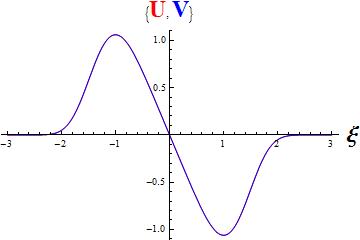
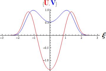
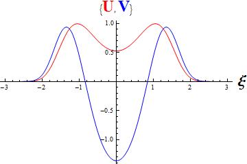
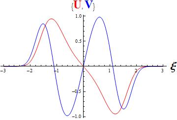
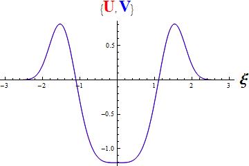
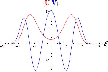
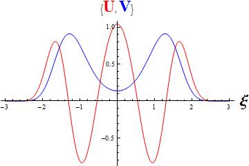
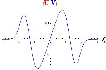
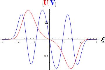
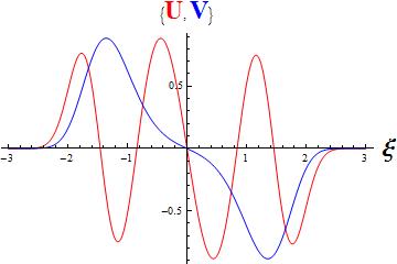
Figure 8: Wave functions for the pure 2:1 oscillator ($\omega=1$) in the plane for principal quantum numbers $N=0,1,\dots,5$. ${\color[rgb]{1,0,0}U}$ is plotted with red and its pair ${\color[rgb]{0,0,1}V}$ in blue.

Energy	Separation const.	degeneracy
$E_{0}=0.228586$	$A_{1}=1$	$d=1$
$E_{1}=2.00297$	$A_{1}=1$	$d=1$
$E_{2}=2.91222$	$A_{1}=-1.7712,A_{1}=3.7712$	$d=2$
$E_{3}=4.10518$	$A_{1}=-3.81344,5.81344$	$d=2$
$E_{4}=4.78076$	$A_{1}=1$	$d=1$
$\tilde{E}_{4}=5.13544$	$A_{1}=-6.89357,8.89357$	$d=2$

Table 2: Numerical results for the coupled 2:1 oscillator + attractive Kepler potential. The separation constant $A_{2}$ is determined by the constraint (4.6). We took $a=1$ and $\omega_{\rho}=1$.

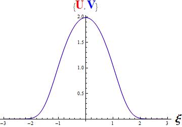
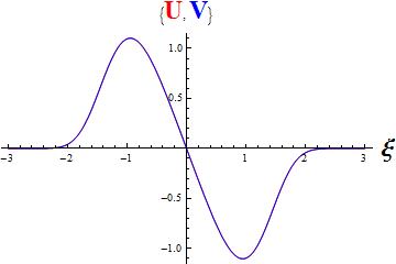
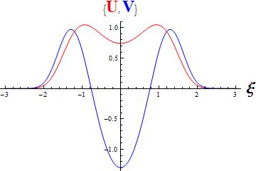
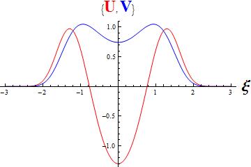
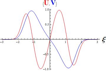
Figure 9: The lowest-energy wave functions of the coupled 2:1 oscillator perturbed with an attractive Kepler potential. $a=1$ and $\omega=1$.

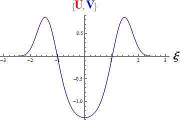
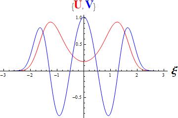
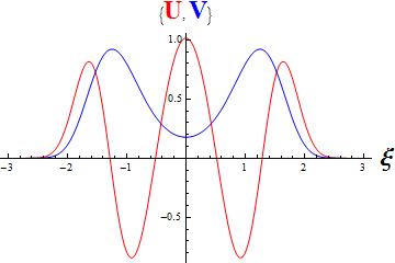
Figure 10: The Kepler perturbation splits the $N=4$ triplet of states of the pure oscillator into a singlet plus a slightly higher-energy doublet, cf. Table 2.

The combined case with repulsive (Coulomb-type) interaction is presented. in Table 3 and on Fig. 11.

Energy	Separ. const.	degener
$E_{0}=2.38668$	$A_{1}=-1$	$d=1$
$E_{1}=4.04956$	$A_{1}=-4.01553,2.01553$	$d=2$
$E_{2}=5.85676$	$A_{1}=-9.14289,7.1428$	$d=2$

Table 3: Numerical results for the coupled oscillator + repulsive Coulomb potential, relevant for Quantum Dots. $a=-1,\omega=1$.

Figure 11: The lowest-energy states for the 2:1 oscillator coupled to a repulsive Coulomb potential, relevant for Quantum Dots.

5 Further separable perturbations

More generally, our trick plainly works for any axial potential which satisfies, in parabolic coordinates, the separability condition (2.38). For example :

1. Let us consider, e.g., the Hartmann potential used in quantum chemistry Hartmann ; KiWi ,

   $$V^{Hartmann}=\frac{a}{\rho^{2}}=\frac{a}{\xi^{2}\eta^{2}}$$ (5.1)

   in (semi)parabolic coordinates. The separability condition (2.38) is satisfied, since

   $$(\xi^{2}+\eta^{2})V=\frac{a}{\xi^{2}}+\frac{a}{\eta^{2}}=f(\xi)+g(\eta).$$ (5.2)

   Eqn. (2.5) provides us with three conserved quantities in involution. The generalized Runge-Lenz-type scalar $K_{z}$ is, in particular, of the form (2.41) and (2.44), respectively, but where the last, additional term is rather

   $$a\,\frac{\xi^{2}-\eta^{2}}{\xi^{2}\eta^{2}}=2a\frac{z}{\rho^{2}}.$$ (5.3)

   The system is separable also in spherical coordinates cf. Hartmann ; KiWi . The spherical Stäckel quantities are (2.22) except for the last contribution to $\underline{w}$ which, fixed by the potential, should read now

   $$\underline{w}=\left(\begin{array}[]{c}0\\ \frac{a}{\sin^{2}\theta}\\ 0\end{array}\right).$$ (5.4)

   The mutually commuting conserved quantities are therefore $H,\,L_{z}^{2}/2-a$, and the modified total angular momentum-square,

   $${\cal L}^{2}=\frac{L^{2}}{2}+\frac{a}{\sin^{2}\theta}\,,$$ (5.5)

   as found before KiWi .

2. Another example is provided by the constant perturbing field ${\bf E}=E\hat{z}$ parallel to the magnetic field considered in the Stark effect Cordani ,

   $$V=Ez=\frac{E}{2}(\xi^{2}-\eta^{2})\quad\Rightarrow\quad(\xi^{2}+\eta^{2})V=\frac{E}{2}(\xi^{4}-\eta^{4}).$$ (5.6)

   The Runge-Lenz type scalar $K_{z}$ is proportional to the projection of the Runge-Lenz vector on the electric field, augmented with a correction term Redmond ,

   $$({\bm{L}}\times{\bm{p}}-a\hat{{\bm{r}}})\cdot{\bf E}-\frac{1}{2}({\bm{r}}\times{\bf E})^{2}.$$ (5.7)

3. General polynomial solutions to (2.38) are obtained Komornik for any integer $n=0,\pm 1,\dots$, $a=\mathop{\rm const}\nolimits$, by

   $$V_{n}=a\,\frac{\xi^{2n}+(-1)^{n+1}\eta^{2n}}{\xi^{2}+\eta^{2}}\,.$$ (5.8)

   which is indeed manifestly separable. On the other hand, the algebraic identity

   $$\xi^{2n+2}+(-1)^{n+2}\eta^{2n+2}=(\xi^{2}-\eta^{2})(\xi^{2n}+(-1)^{n+1}\eta^{2n})-(\xi^{2}\eta^{2})(\xi^{2n-2}+(-1)^{n}\eta^{2n-2})$$

   translates into $V_{n+1}=2z\,V_{n}-\rho^{2}\,V_{n-1},$ proving by induction that $V_{n}$ is also axially symmetric. Similarly, the identity

   $$\underbrace{\xi^{2n+2}+(-1)^{n+1}\eta^{2n+2}}_{\widetilde{V}_{n+1}}=\underbrace{(\xi^{2}-\eta^{2})}_{2z}\underbrace{(\xi^{2n}+(-1)^{n}\eta^{2n})}_{\widetilde{V}_{n}}+\underbrace{(\xi^{2}\eta^{2})}_{\rho^{2}}\underbrace{(\xi^{2n-2}+(-1)^{n-1}\eta^{2n-2})}_{\widetilde{V}_{n-1}}$$

   shows that

   $$\widetilde{V}_{n}=a\,\frac{\xi^{2n}+(-1)^{n}\eta^{2n}}{\xi^{2}+\eta^{2}}$$ (5.9)

   is also separable and axially symmetric, providing us with a second doubly-infinite tower of axially symmetric separable potentials.

   For $n=-1$ we get Makar ; KiWi

   $$\widetilde{V}=\frac{1}{2r}\left(\frac{1}{\xi^{2}}-\frac{1}{\eta^{2}}\right)=-\frac{1}{r}\frac{z}{\rho^{2}}=-\frac{\cos\theta}{r^{2}\sin^{2}\theta}\,.$$ (5.10)

   Some further interesting cases are listed in Table 4.

   $n=0$	$V=0$	trivial
   $n=1$	$V=1$	trivial
   $n=2$	$V=Ez$	Stark effect
   $n=3$	$V=\rho^{2}+2z^{2}$	1:2 oscillator
   $n=-1$	$V=\displaystyle\frac{1}{\rho^{2}}=\displaystyle\frac{1}{r^{2}\sin^{2}\theta}$	Hartmann potential
   $n=0$	$\widetilde{V}=\displaystyle\frac{1}{r}$	Coulomb
   $n=1$	$\widetilde{V}=\displaystyle\frac{2z}{r}$	?
   $n=-1$	$\widetilde{V}=\displaystyle\frac{z}{r\rho^{2}}=\displaystyle\frac{\cos\theta}{r^{2}\sin^{2}\theta}$	Makarov et al.

   Table 4: Some potentials which are separable in parabolic coordinates.

Similar calculations show that, in the two remaining coordinate systems, no perturbing potential can be added while preserving separability, though.

6 Conclusion

To explain the findings of Simonović et al. about the separability of quantum dots Simon has been to trade first the constant magnetic field for a pure axially symmetric oscillator by switching to rotating coordinates.

The hydrogen atom is separable in four appropriate coordinate systems Cordani ; then we asked : “which potentials can be added so that separability is preserved in one of those coordinates ?” The answer we found says that, apart of the expected spherical case, separability can be achieved in parabolic coordinates for any axial potential which satisfies the separability condition (2.38).

For the harmonic trap considered in the QD problem Simon this requires a 2:1 anisotropy, cf. (2.39).

To gain further insight, we found it convenient to first restrict the system to the vertical $x-z$ plane. Then, removing the constraint $L_{z}=p_{\varphi}=0$, allowed us to recover the 3D motion and its properties.

More general separable solutions, beyond the 2:1 oscillator, arise, though, some of them listed in Table I . These cases can plainly be combined due to the additivity of both the functions $f(\xi)$ and $g(\eta)$ and of the potentials cf. (2.38). One can, for example, put the QD into an additional electric field parallel to the magnetic one, as well as adding the Hartmann potential, etc. (A harmonic part is always necessary, though, due to the magnetic field).

Our strategy has been to start with the pure Kepler problem Cordani and then inquire what potential can be added such that separability in (semi)parabolic coordinates is preserved. In the same spirit, we viewed the “Runge-Lenz-type” conserved quantity $K_{z}$ in (2.41) as the Keplerian expression [represented by the first and the third terms], “corrected” by the third one due to the oscillator.

But we could have also started at the other end, i.e., with the pure anisotropic oscillator, which is separable, for $2:1$ ratio of the frequencies, in both Cartesian and (semi)parabolic coordinates Makar ; Boyer . Then we could have observed that separability in (semi)parabolic coordinates is consistent with a Kepler potential of arbitrary strength, viewed as a perturbation of our initial oscillator. We could also view (2.41) as the conserved quantity related to oscillator-separability [represented by the first and the third terms], “corrected” by the middle one, required due to the Keplerian perturbation. We mention that our problem here can further be generalized by including magnetic charges Krivonos .

Note added After this paper has been accepted, we received a message from J-W van Holten vanHolten , pointing out that our results can also be derived using the covariant framework of Ref. Killing based on Killing tensors. Our conserved quantity (3.32) is indeed associated to a fourth-rank Killing tensor – the only previously known examples being those discussed in Ref. 4Killing .

- (1) N. S. Simonović and R. G. Nazmitdinov, “Hidden symmetries of two-electron quantum dots in a magnetic field,” Phys. Rev. B67, 041305(R) (2003);
- (2) N. S. Simonovic and R. G. Nazmitdinov “Dynamical screening of the Coulomb interaction for two confined electrons in a magnetic field,” Phys. Rev. A 78, 032115 (2008) [arXiv:0809.4285]; R. G. Nazmitdinov and N. S. Simonovic, “Finite-thickness effects in ground-state transitions of two-electron quantum dots,” Phys. Rev. B 76, 193306 (2007) [arXiv:0711.1246]
- (3) G. W. Gibbons, C. N. Pope “Kohn’s Theorem, Larmor’s Equivalence Principle and the Newton-Hooke Group,” Annals of Physics 326, 1760 (2011) [arXiv:1010.2455]. P. M. Zhang and P. A. Horvathy, “Kohn’s theorem and Galilean symmetry,” Phys. Lett. B702 (2011) 177
- (4) P. M. Zhang, P. A. Horvathy, K. Andrzejewski, J. Gonera and P. Kosinski, “Newton-Hooke type symmetry of anisotropic oscillators,” Ann. Phys. Ann. Phys. 333, 335 (2013). [arXiv:1207.2875 [hep-th]].
- (5) Y. Alhassid, E. A. Hinds and D. Meschede, “Dynamical Symmetries of the Perturbed Hydrogen Atom : the van der Waals Interaction,” Phys. Rev. Lett. 59 (1987) 1545; K. Ganesan and M. Lakshmanan, “Comment on “Dynamical Symmetries of the Perturbed Hydrogen Atom : the van der Waals Interaction,””, Phys. Rev. Lett. 629 (1989) 232.
- (6) R. Blümel, C. Kappler, W. Quint, and J. Walter, “Chaos and order of laser-cooled ions in a Paul trap,” Phys. Rev. A40, 808 (1989). Erratum: Phys. Rev. A 46, 8034 (1992).
- (7) B. Cordani, “The Kepler Problem,” Birkhäuser (2003).
- (8) S. Benenti, “Intrinsic characterization of the variable separation in the Hamilton-Jacobi equation,” J. Math. Phys. 38, 6578 (1997); S. Benenti, C. Chanu, G. Rastelli, “Remarks on the connection between the additive separation of the Hamilton-Jacobi equation and the multiplicative separation of the Schrödinger equation,” Tech. Rep. 22, Quaderni del Dipartimento di Matematica – Università di Torino (2001).
- (9) L.P. Eisenhart, “Separable systems in Euclidean space,” Phys. Rev. 45, 427 (1934).
- (10) A.A. Makarov, J.A. Smorodinsky, Kh. Valiev, P. Winternitz, “A systematic search for nonrelativistic systems with dynamical symmetries. Part I: the integrals of motion,” Il Nuovo Cimento A52, 1061 (1967); P. Winternitz, Ya. A. Smorodinskii, M. Uhlir and I. Fris, “Symmetry Groups in Classical and Quantum Mechanics,” Soviet Journal of Nuclear Physics 4, 444 (1967) [in Russian: JNP 4, 625 (1966)].
- (11) C. P. Boyer and K. B. Wolf, “The 2:1 Anisotropic Oscillator, Separation of Variables and Symmetry Group in Bargmann Space,” J. Math. Phys. 16 (1975) 2215.
- (12) J.M. Jauch and E. L. Hill, “On the problem of degeneracy in Quantum Mechanics,” Phys. Rev. 57, 641 (1940).
- (13) A. Cisneros and H. V. McIntosh, “Symmetry of the two-dimensional hydrogen atom,” J. Math. Phys. 10, 277 (1969).
- (14) V.I. Arnold, Mathematical Methods of Classical Mechanics, Springer, New York (1989). Bertrand’s theorem has originally been stated by J. Bertrand, Compt. Rend. 77, 849 (1873).
- (15) T. T. Truong, “A Weyl quantization of anharmonic oscillators,” J. Math. Phys. 16 (1975) 1034. The solutions of Eqn. (4.7), studied analytically, can be related to the confluent Heun equations.
- (16) L. Landau and E. Lifshitz, “Quantum Mechanics. Non-Relativistic Theory,” Vol. 3 of Course of Theoretical Physics. 3rd Edition: Pergamon Press (1977). & 97, pp. 128.
- (17) H. Hartmann, “Die Bewegung eines Körpers in einem ringförmigen Potentialfeld,” Theor. Chim. Acta (Berl.) 24, 201 (1972); M. Kibler and T. Negadi, “Motion of a particle in a ring-shaped potential : an approach via a nonbijective canonical transformation,” Intl. Journ. Quantum Chem. 26, 405 (1984).
- (18) M. Kibler and P. Winternitz, “Dynamical invariance algebra of the Hartmann potential,” J. Phys. A 20, 4097 (1987).
- (19) P. J. Redmond, “Generalization of the Runge-Lenz vector in the presence of an electric field,” Phys. Rev. 133, B1352 (1964).
- (20) V. Komornik (private communication).
- (21) S. Krivonos, A. Nersessian and V. Ohanyan, “Multi-center MICZ-Kepler system, supersymmetry and integrability,” Phys. Rev. D 75, 085002 (2007) [hep-th/0611268].
- (22) J. W. van Holten, private communication (2013).
- (23) J. W. van Holten, “Covariant Hamiltonian dynamics,” Phys. Rev. D 75 (2007) 025027 [hep-th/0612216].
- (24) G. W. Gibbons, T. Houri, D. Kubiznak and C. M. Warnick, “Some Spacetimes with Higher Rank Killing-Stäckel Tensors,” Phys. Lett. B 700 (2011) 68 [arXiv:1103.5366 [gr-qc]]; A. Galajinsky, “Higher rank Killing tensors and Calogero model,” Phys. Rev. D 85 (2012) 085002 [arXiv:1201.3085 [hep-th]];