Quasi-energies, parametric resonances, and stability limits in ac-driven $\mathcal{PT}$-symmetric systems

Abstract

We introduce a simple model for implementing the concepts of quasi-energy and parametric resonances (PRs) in systems with the $\mathcal{PT}$ symmetry, i.e., a pair of coupled and mutually balanced gain and loss elements. The parametric (ac) forcing is applied through periodic modulation of the coefficient accounting for the coupling of the two degrees of freedom. The system may be realized in optics as a dual-core waveguide with the gain and loss applied to different cores, and the thickness of the gap between them subject to a periodic modulation. The onset and development of the parametric instability for a small forcing amplitude ($V_{1}$) is studied in an analytical form. The full dynamical chart of the system is generated by systematic simulations. At sufficiently large values of the forcing frequency, $\omega$, tongues of the parametric instability originate, with the increase of $V_{1}$, as predicted by the analysis. However, the tongues following further increase of $V_{1}$ feature a pattern drastically different from that in usual (non-$\mathcal{PT}$) parametrically driven systems: instead of bending down to larger values of the dc coupling constant, $V_{0}$, they maintain a direction parallel to the $V_{1}$ axis. The system of the parallel tongues gets dense with the decrease of $\omega$, merging into a complex small-scale structure of alternating regions of stability and instability. The cases of $\omega\rightarrow 0$ and $\omega\rightarrow\infty$ are studied analytically by means of the adiabatic and averaging approximation, respectively. The cubic nonlinearity, if added to the system, alters the picture, destabilizing many originally robust dynamical regimes, and stabilizing some which were unstable.

Recently, a great deal of interest has been drawn to systems featuring the $\mathcal{PT}$ (parity-time) symmetry. Originally, they were introduced as quantum systems with spatially separated and symmetrically placed linear gain and loss. A fundamental property of non-Hermitian $\mathcal{PT}$-symmetric Hamiltonians is the fact that their spectra remain purely real, like in the case of the usual Hermitian Hamiltonians, provided that the strength of the non-Hermitian part of the Hamiltonian, $\gamma$, does not exceed a certain critical value, $\gamma_{\mathrm{cr}}$, at which the $\mathcal{PT}$ symmetry breaks down. Such linear systems were recently implemented experimentally in optics, due to the fact that the paraxial propagation equation for electromagnetic waves can emulate the quantum-mechanical Schrödinger equation. In particular, the $\mathcal{PT}$-symmetric quantum system may be emulated by waveguides with spatially separated mutually balanced gain and loss elements. Additional interest to the optical realizations of the $\mathcal{PT}$ symmetry has been drawn by the possibility to implement this setting in nonlinear waveguides. Unlike the ordinary models of nonlinear dissipative systems, where stable modes exist as isolated attractors, in $\mathcal{PT}$-symmetric systems they emerge in continuous families, similar to what is commonly known about conservative nonlinear systems. However, the increase of the gain-loss coefficient, $\gamma$, leads to the shrinkage of existence and stability regions for the $\mathcal{PT}$-symmetric modes, which completely vanish at some $\gamma=\gamma_{\mathrm{cr}}$. Especially convenient for the study of such solutions are models of dual-core couplers, with the balanced gain and loss applied to different cores, and the cubic nonlinearity acting in both. The objective of the present work is to extend the well-known concepts of quasi-energy and parametric resonances (PRs) to $\mathcal{PT}$-symmetric systems. In terms of the coupler model, the parametric drive (with ac amplitude $V_{1}$ and dc amplitude $V_{0}$) can be implemented by making the thickness of the gap between the two cores in the coupler a periodic function of the evolution variable (propagation distance, in terms of optics), with frequency $\omega$. Using a combination of analytical and numerical methods, we produce the full dynamical chart for both linear and nonlinear versions of the system in the plane of $\left(V_{1},V_{0}\right)$ for different values of $\omega$. The charts feature tongues of parametric instability, whose shape has some significant differences from that predicted by the classical theory of the PR in conservative systems. In addition, the cases of small and large $\omega$ are studied by means of the adiabatic and averaging approximations, respectively.

I Introduction and the model

A commonly known principle of quantum mechanics is that operators representing physical variables, including the Hamiltonian, must be Hermitian, to guarantee the reality of the respective spectra. Recently, it was found that the class of physically acceptable Hamiltonians may be extended by admitting operators with anti-Hermitian [dissipative and antidissipative (gain)] parts, if they commute with the $\mathcal{PT}$ (parity-time) transformation Bender_review . The spectrum of such a $\mathcal{PT}$-invariant Hamiltonian may be purely real, provided that the strength of the anti-Hermitian part, $\gamma$, does not exceeds a critical value, $\gamma_{\mathrm{cr}}$, at which complex eigenvalues emerge. In the simplest form, a $\mathcal{PT}$-invariant Hamiltonian contains a complex potential in which the real part is an even function of coordinates, while the imaginary part is odd.

While in the quantum theory this concept remains a rather abstract one, the similarity of the quantum-mechanical Schrödinger equation to the paraxial propagation equation in optics has suggested a possibility to emulate the $\mathcal{PT}$-symmetry in optical waveguides with symmetrically placed mutually balanced gain and loss elements. This implementation was proposed theoretically Muga and then demonstrated in experiments experiment . Recently, another experimental realization of the $\mathcal{PT}$ symmetry was reported in a system of coupled electronic oscillators Kottos . There is a possibility to realize such a setting in Bose-Einstein condensates BEC too.

These possibilities have drawn a great deal of interest to the analysis of various $\mathcal{PT}$-symmetric dynamical models special-issues ; review . In particular, the natural occurrence of the self-focusing in optical media stimulated the study of nonlinear effects in such systems. The interplay of the paraxial diffraction, Kerr nonlinearity, and a spatially periodic complex potential, which represents the $\mathcal{PT}$-symmetric part of the system, gives rise to bright solitons Musslimani2008 , whose stability was rigorously analyzed in Ref. Yang . Dark solitons have been predicted too in this context, assuming the self-defocusing Kerr nonlinearity dark . In addition, bright solitons have been predicted in $\mathcal{PT}$-symmetric systems with the quadratic (second-harmonic-generating) nonlinearity chi2 . Systems of another type, which readily maintain $\mathcal{PT}$-symmetric solitons, and actually make it possible to obtain such solutions and their stability conditions in an exact analytical form, are provided by models of linearly-coupled dual-core waveguides, with the balanced gain and loss applied to the two cores, and the intrinsic Kerr nonlinearity present in each one dual -dark-coupler .

Further, nonlinear modes were studied in many discrete $\mathcal{PT}$-symmetric systems with the cubic nonlinearity. These include linear discrete and circular circular chains of coupled $\mathcal{PT}$ elements and aggregates of coupled $\mathcal{PT}$-symmetric oligomers (dimers Hadi , quadrimers, etc.) KPZ . General features of the dynamics in $\mathcal{PT}$-symmetric lattices of single-component nonlinear $\mathcal{PT}$-symmetric lattices have been recently considered in Ref. pelinov . Related to these models are systems featuring discrete $\mathcal{PT}$-balanced elements embedded into continuous nonlinear conservative media Wunner ; Thaw , which, in particular, allow one to find exact solutions for solitons pinned to the $\mathcal{PT}$-symmetric dipole Thaw .

The inclusion of the Kerr nonlinearity into the conservative part of the system suggests that its gain-and-loss part can be made nonlinear too, by adopting mutually balanced cubic gain and loss terms  AKKZ ; Canberra ; rudy . Effects of combined linear and nonlinear $\mathcal{PT}$ terms on the existence and stability of solitons were studied in combined .

In the usual nonlinear dissipative systems, stable dynamical regimes exist as isolated solutions (attractors), such as limit cycles or strange attractors SA in discrete settings, or dissipative solitons in dissipative media PhysicaD . On the contrary to that, in $\mathcal{PT}$-symmetric systems stable modes form continuous families, similar to the generic situation in conservative systems. However, the increase of the gain-loss coefficient ($\gamma$) in the $\mathcal{PT}$-symmetric system leads to shrinkage of existence and stability domains for the families, which eventually vanish at $\gamma=\gamma_{\mathrm{cr}}$.

In many cases, quantum systems are driven by time-periodic (ac) external forces. In that case, the eigenstates are characterized by particular values of the quasi-energy, defined as per the Floquet theorem, see, e.g., Ref. Floquet . A related concept is the parametric resonance (PR) in linear and nonlinear systems subject to the action of the parametric drive LL . In the context of $\mathcal{PT}$-symmetric systems, it is interesting to analyze the realization of the quasi-energy and PRs in ac-driven systems, both linear and nonlinear ones, including mutually balanced gain and loss terms. This analysis is the subject of the present work. We perform it in the framework of a basic model with two degrees of freedom (a dimer), represented by complex amplitudes $\psi_{A}$ and $\psi_{B}$, and the coupling containing an ac-modulated term, which represents the parametric drive:

$$i\frac{d}{dt}\psi_{A} = i\psi_{A}+\left[V_{0}+2V_{1}\cos\left(\omega t\right)\right]\psi_{B}+\chi|\psi_{A}|^{2}\psi_{A},$$

$$i\frac{d}{dt}\psi_{B} = -i\psi_{B}+\left[V_{0}+2V_{1}\cos\left(\omega t\right)\right]\psi_{A}+\chi|\psi_{B}|^{2}\psi_{B}.$$ (1)

Here the equal gain and loss coefficients in the equations for $\psi_{A}$ and $\psi_{B}$ are scaled to be $\gamma\equiv 1$, $V_{0}$ and $V_{1}$ are strengths of the constant (dc) and ac-modulated couplings, $\omega$ is the modulation frequency, and $\chi$ is the nonlinearity coefficient, which may be taken as $\chi=0$ or $\chi\equiv 1$ in the linear and nonlinear versions of the system. Note that by the complex conjugation and replacing $\psi_{A},\psi_{B}$ $\rightarrow$ $-\psi_{A}^{\ast},\psi_{B}^{\ast}$ Eqs. (1) with $\chi=\pm 1$ are transformed into each other, therefore we do not consider $\chi=-1$. Also, by an obvious transformation $\psi_{A},\psi_{B}\rightarrow\psi_{A},-\psi_{B}$, it is possible to reverse the sign of $V_{0}$, and shift $t\rightarrow t+\pi/\omega$ can independently reverse the sign of $V_{1}$, therefore we can fix both $V_{0}$ and $V_{1}$ to be positive.

According to the concept of the quasi-energy, quasi-stationary solutions to Eqs. (1) for $\omega\neq 0$ are sought for as

$$\psi_{A}(t)=\exp\left(-iEt\right)\Psi_{A}(t),~{}\psi_{B}(t)=\exp\left(-iEt\right)\Psi_{B}(t)$$ (2)

where $\Psi_{A,B}(t)$ are periodic functions with period $2\pi/\omega$, and the quasi-energy $E$ belongs to interval $0<E<2\pi/\omega$. A corollary of Eqs. (1) is the balance equation for the total power in the presence of the mutually symmetric gain and loss pelinov

$$\frac{d}{dt}\left(|\psi_{A}|^{2}+|\psi_{B}|^{2}\right)=2\left(|\psi_{A}|^{2}-|\psi_{B}|^{2}\right).$$ (3)

This system can be implemented as a model of a dual-core optical waveguide operating in the CW (continuous-wave) regime, so that Eqs. (1) do not include terms accounting for the transverse diffraction or group-velocity dispersion, in the spatial-domain and temporal-domain realizations, respectively. Variable $t$ is actually the propagation distance, and the ac modulation represents periodic variation of the thickness of the gap separating the cores Sydney . As suggested in Refs. dual , terms $\pm i\psi_{A,B}$ in Eqs. (1) represent the gain and loss applied to the two cores. A similar system, without the ac-modulating terms, but with the addition of cubic gain and loss terms, was proposed as a model of a $\mathcal{PT}$-symmetric dimer in Ref. Canberra .

The main issue considered in this work is the effect of the $\mathcal{PT}$ symmetry on PRs in the framework of the linear and nonlinear versions of system (1). First, in Sections II.A-B we develop an analytical approach for the case of moderate $\omega$, predicting at what values of $V_{0}$ the ac drive with fixed $\omega$ gives rise to the PR at infinitesimally small $V_{1}$, and how tongues of the parametric instability expand with the increase of $V_{1}$. Comprehensive dynamical charts of the linearized version of system (1) and the full  nonlinear system, built on the basis of systematic numerical simulations, are presented in Sections II.C-D, respectively. The structure of the charts at large $V_{1}$ is very different from the picture of PRs in usual (non-$\mathcal{PT}$) driven dynamical systems. In Section III we present, in a brief form, solutions of the system for slow (small $\omega$) and fast (large $\omega$) time-periodic modulations, which can be treated, respectively, by means of the adiabatic and averaging approximations. The paper is concluded by Section IV.

II The analysis for moderate driving frequencies $\omega$

II.1 Perturbative analysis of the linear system

With a small amplitude of the ac drive, $V_{1}$, a perturbative solution to the linearized version of Eqs. (1), with quasi-frequency $E$ (or quasi-energy, in terms of quantum $\mathcal{PT}$-symmetric systems), is looked for in the form of Eq. (2), adopting the lowest-order truncation for the Fourier expansion of the $t$-periodic amplitudes LL ,

$$\Psi_{A,B}(t)=\Psi_{A,B}^{(0)}+\Psi_{A,B}^{(+)}e^{-i\omega t}+\Psi_{A,B}^{(-)}e^{+i\omega t},$$ (4)

with constants $\Psi_{A}^{(0,\pm)},\Psi_{B}^{(0,\pm)}$. Substituting this ansatz into Eqs. (1) and keeping, in line with the form of truncation (4), the zeroth and first harmonics in the ensuing expansion, gives rise to a system of linear homogeneous equations for the vectorial set of six amplitudes,

$$\mathbf{\Psi}=\left\{\Psi_{A}^{(0)},\ \Psi_{A}^{(+)},\ \Psi_{A}^{(-)},\ \Psi_{B}^{(0)},\ \Psi_{B}^{(+)},\ \Psi_{B}^{(-)}\right\}.$$ (5)

Nontrivial solutions exist under the condition that the determinant of the system vanishes, which leads to the following equation for $E$:

$$\left|\begin{array}[]{cccccc}i-E&0&0&V_{0}&V_{1}&V_{1}\\ 0&i-E-\omega&0&V_{1}&V_{0}&0\\ 0&0&i-E+\omega&V_{1}&0&V_{0}\\ V_{0}&V_{1}&V_{1}&-i-E&0&0\\ V_{1}&V_{0}&0&0&-i-E-\omega&0\\ V_{1}&0&V_{0}&0&0&-i-E+\omega\end{array}\right|=0~{}.$$ (6)

Each eigenvalue $E$ is associated with eigenvector $\mathbf{\Psi}$ of matrix (6). Complex solutions of Eq. (6) for $E$ imply instability of the linear system due to the spontaneous breaking of the $\mathcal{PT}$ symmetry, or excitation of a PR, or an interplay of both mechanisms (as shown below, all these cases are possible). Real eigenvalues $E$ correspond to stable oscillatory solutions.

In the zeroth-order approximation, $V_{1}=0$, Eq. (6) yields an obvious result: the spectrum remains real under the condition

$$V_{0}^{2}>\left(V_{0}^{2}\right)_{\min}\equiv 1$$ (7)

[more explicitly, $\left(V_{0}^{2}\right)_{\min}=\gamma^{2}$, if scaling $\gamma\equiv 1$ for the gain-loss coefficient is not fixed]. In this approximation, the six eigenvalues are

$$E=\pm\sqrt{V_{0}^{2}-1},E=\pm\omega\pm\sqrt{V_{0}^{2}-1},$$ (8)

where different $\pm$ signs are mutually independent.

Stability and instability areas in the plane of the ac and dc coupling strengths, $\left(V_{1},V_{0}\right)$, at four different values of the driving frequency,

$$\omega=0.4,0.8,1.5,2\sqrt{3}\approx 3.46,$$ (9)

as predicted by a numerical solution of algebraic equation (6), is displayed in Fig. 1. The plots also show stability areas (covered by dots) as obtained in Section III by means of systematic direct simulations of the linear version of Eqs. (1), i.e., the one with $\chi=0$. Circles on the vertical axis in Fig. 1 corresponds to parametric resonances, as described in the next subsection.

Figure 1: Dark and white backgrounds represent, respectively, areas of stability and instability of the linear version of system (1) with $\chi=0$, as predicted by the numerical solution of perturbative equation (6), in the parameter plane of $\left(V_{1},V_{0}\right)$ at several fixed values of $\omega$ (the equation produces solely real eigenvalues $E$ in the stable areas). The plots are superimposed with dots denoting parameter values for which direct simulations of the linear version of Eqs. (1) demonstrate stability, unstable solutions populating areas in the parameter plane which are not covered by dots. The dotted grid was built with steps $\Delta V_{1}=\Delta V_{0}=0.125$. Small circles on the left vertical axes, corresponding to $V_{1}\rightarrow 0$, correspond to discrete points at which the parametric resonances are predicted by Eq. (10).

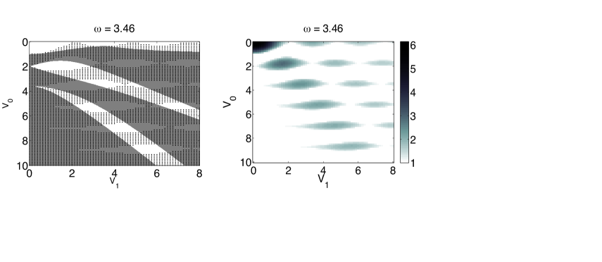
Figure 2: The same as the bottom right panel of Fig. 1 but the dots are generated by calculating the Floquet multipliers (eigenvalues) of the monodromy matrix $J_{P}$. The right panel shows the magnitude of the maximal multiplier in order to demonstrate the growth rate of the instabilities. The white regions of the right panel indicate that all the Floquet multipliers are of modulus one indicating stability.

II.2 Parametric resonances

In the limit of $V_{1}\rightarrow 0$, when the eigenfrequency of free oscillations in the linearized system is $E=\sqrt{V_{0}^{2}-1}$, see Eq. (8), the standard theory LL produces the PR (i.e., the onset of the instability of the linear system, different from the instability due to breaking of the $\mathcal{PT}$ symmetry) at the following values of the driving frequency:

$$\omega_{\mathrm{res}}^{(n)}=\frac{2}{n}\sqrt{V_{0}^{2}-1},$$ (10)

where $n=1,2,3,...$ is the order of the resonance. Thus, for given driving frequency $\omega$, Eq. (10) predicts the resonance at

$$\left(V_{0}\right)_{\mathrm{res}}^{(n)}=\sqrt{1+\left(n\omega/2\right)^{2}}.$$ (11)

In Fig. 1, circles on the vertical axis in each plot mark positions of the PR as predicted by Eq. (11).

Note that in the case of $\omega=0.4$, Eq. (11) yields values

$$\left(V_{0}\right)_{\mathrm{res}}^{(1)}=\sqrt{1.04}\approx 1.02,~{}\left(V_{0}\right)_{\mathrm{res}}^{(2)}=\sqrt{1.16}\approx 1.08,$$ (12)

which are close to the above-mentioned critical value, $\left(V_{0}\right)_{\min}=1$, induced by the balanced combination of the gain and loss terms, see Eq. (7). The wide and narrow instability stripes, observed in the panel of Fig. 1 corresponding to $\omega=0.4$, originate from two critical values (12) at small values of $V_{1}$. This situation actually implies a merger of the $\mathcal{PT}$-breaking and PR-induced instabilities for relatively small values of $\omega$.

At larger $\omega$, the $\mathcal{PT}$ and PR instabilities are clearly separated as $V_{1}\rightarrow 0$. For instance, at $\omega=2\sqrt{3}\approx\allowbreak 3.46$, Eq. (11) yields $\left(V_{0}\right)_{\mathrm{res}}^{(1)}=2$ for the fundamental parametric resonance ($n=1$). In accordance with this, the respective panel of Fig. 1 features a separate instability tongue, originating, at small $V_{1}$, from point $V_{0}=2$, and expanding with the increase of $V_{1}$. The additional tongue observed in the same panel, originating from $V_{0}=\sqrt{13}\approx\allowbreak 3.6$ at $V_{1}=0$, is predicted by Eq. (11) with $n=2$. These tongues are quite similar to those known in the usual (non-$\mathcal{PT}$) model of the parametric instability.

II.3 Direct simulations of the linear system on the parameter grid

To produce an accurate stability chart for the linear version of the underlying system, i.e., Eqs. (1) with $\chi=0$, we ran systematic simulations of the equations on a square grid in the plane of $\left(V_{1},V_{0}\right)$ with limits $0\leq V_{1}\leq 8$, $0\leq V_{0}\leq 10$ and steps $\Delta V_{1}=\Delta V_{0}=0.125$. We show results at the four fixed values of the driving frequency from set (9). Initial values $\left\{\psi_{A}(0),\psi_{B}(0)\right\}$ for each run of the simulations were calculated as per Eqs. (2) and (4), with set (5) calculated as an eigenvector of matrix (6). The simulations were performed by means of a standard fourth-order Runge-Kutta code. To check the accuracy of the calculations, we verified that the numerical solutions would satisfy balance equation (3).

To distinguish between stable and unstable solutions in the present system, we checked whether the maximum of $|\psi_{A}(t)|$ or $|\psi_{B}(t)|$ would double after a sufficiently long period of time, in comparison to the modulation period, $2\pi/\omega$. It has been found that the lack of the doubling is an appropriate indicator of the stability of a given solution (in other words, the solutions which could be identified as stable ones would never double their largest absolute value). Each parameter set categorized as stable is marked by a dot in Fig. 1. Unstable solutions were identified as those breaking the above-mentioned no-doubling condition, which was followed by visual checks, which corroborate that the so identified unstable solutions indeed suffer blowup. In Fig. 1, unstable solutions are represented by missing dots on the selected grid.

The stability of $t$-periodic solutions can also be numerically analyzed by computing the eigenvalues of the monodromy matrix $J_{P}$ for small perturbations around the given solution perturbation (in the case of the linear problem, this effectively amounts to the stability of the zero solution). Writing (1) with $\chi=0$ as a system of four real equations with Jacobian $J_{F}(t)$ implies that $J_{P}$, the Jacobian of the Poincaré map, satisfies the variational equation

$$\frac{d}{dt}(J_{P})=J_{F}(J_{P})$$ (13)

with initial condition $J_{P}(0)=Id$. Solving (13) and computing the eigenvalues of $J_{P}(t=2\pi/\omega)$ gives the Floquet multipliers which indicate instability if any of the multipliers have modulus greater than one. In Fig. 2 we show that this Floquet multiplier calculation predicts the exact same (in)stability intervals as that which we observed using the doubling condition of our direct integration as explained above.

Figure 1 clearly demonstrates both similarities and nontrivial differences between the present stability charts and those well known in the PR theory. Indeed, different numerical stability tongues originating at $V_{1}=0$ do not bend down, as in the usual theory, but keep the direction parallel to the axis of $V_{1}$. This difference suggests that the truncation adopted in Eq. (4) becomes irrelevant at large $V_{1}$, as a larger number of harmonics get involved into the dynamics, as corroborated by spectra of particular solutions displayed below. With the decrease of $\omega$, the number of tongues becomes large, while their widths and gaps between adjacent ones get smaller. At small $\omega$, the stability chart features a complex small-scale structure, which has no counterpart in the ordinary PR theory. It is important to point out that, while the quasi-energy-based analysis presented in Section II.A is expected (and indeed found in Fig. 1) to be valid for small $V_{1}$, the PR theory of section II.B is relevant in a different limit. In particular, it accurately captures the dynamics at large $\omega$, where the PR points are no longer clustered, and their tongues shrink accordingly. It is clearly observed in Fig. 1 that the horizontal tongues for the cases of, e.g., $\omega=1.5$ and $3.46$ naturally emanate from the PR points of $V_{1}\rightarrow 0$. An additional relevant point to mention in that light is that higher-order resonances appear to be initiated “deeper” along the $V_{1}$ axis, although this observation may be affected by a finite extension of our simulations, and of a weak growth rate of these instabilities at small $V_{1}$.

Figure 3 shows characteristic examples of the solutions for select combinations of parameter values, both stable (quasi-periodic solutions) and unstable (growing ones). Due to the presence of the gain in the system, unstable solutions grow indefinitely, with (at most) an exponential rate pelinov . As a result, at some point in time, after the temporal interval displayed in respective panels of Fig. 3, each amplitude increases rapidly (eventually the evolution accrues numerical errors).

Figure 3: Solutions $|\psi_{A}(t)|,|\psi_{B}(t)|$ produced by the numerical simulations of the linear version of Eqs. (1) for parameter values corresponding to a vertical cut in Fig. 1 at $\omega=0.4$ and $V_{1}=3.25$. These plots confirm that actually present black dots and missing ones (empty sites of the grid) in Fig. 1 represent stable and unstable solutions, respectively. Values of $V_{0}$ corresponding to the left and right columns (from top to bottom) are $0,0.5,1,3,3.5$, $4$, and $5.5,6,6.5,7.5,8,8.5$, respectively.

For a few stable oscillatory solutions, Fig. 4 shows the power spectra generated by means of the DFFT (discrete fast Fourier transform),

$$\mathrm{power~{}}_{A,B}(f_{k})=\left|\frac{1}{N}\sum_{j=1}^{N}\psi_{A,B}(t_{j})\exp\left(2\pi i\frac{(j-1)k}{N}\right)\right|^{2},$$ (14)

where $t_{j}=j\Delta t$, $t_{N}$ is the total integration time, and $f_{k}\in\frac{1}{N\Delta t}\left\{1,\dots,N/2\right\}$ for even $N$. All the spectra show a prominent peak at the driving frequency, $\omega/\left(2\pi\right)$. One also observes a set of weaker higher-frequency peaks corresponding to the frequency multiplication by the parametric drive.

Figure 4: For $\omega=0.4$, plotted on the logarithmic scale of the frequency are power spectra computed as per Eq. (14) for the following values of the parameters: $(V_{1},V_{0})=$ $(3.25,0.5)$ in the top left, $(3.25,3.5)$ in the bottom left, $(3.25,6)$ in the top right, and $(3.25,7.5)$ in the bottom right. The frequency in the plots is $f$ defined in Eq. (14), and the power spectra for both components of stable solutions completely overlap. The corresponding solutions $\psi_{A,B}(t)$ are displayed in Fig. 3. A prominent peak is found at frequency $0.0637=(\omega=0.4)/2\pi$.

To resolve the higher frequencies (smaller periods), we have performed the FFT on smaller windows. For example, within the first few seconds of the simulations for small $\omega$, we would observe a dominant frequency in the spectrum consistent with the prediction, $f=\sqrt{(V_{0}+2V_{1})^{2}-1}/(2\pi)$, given by Eq. (8) with $\omega=0$. As $\psi_{A}(t)$ and $\psi_{B}(t)$ evolve in time, the high frequencies lead to modulations. For parameter values $\left(V_{0},V_{1}\right)$ which are buried deepest in stability regions in Fig. 1, the solutions feature the least amount of such fluctuations at high frequencies. These fluctuations account for the small-amplitude pattern in the high-frequency part of the spectra in Fig. 4, which appears when the FFT is performed on a large interval, such as $[0,250]$. All of the frequencies which appear in Fig. 4 are linear combinations of those predicted at $\omega=0$ and the driving frequency, $\omega/\left(2\pi\right)$.

II.4 The nonlinear propagation

As indicated above, the initial values of $\left(\psi_{A},\psi_{B}\right)$, used in the simulations of the linear version of Eqs. (1), were generated as per Eqs. (2) and (4), into which eigenvectors (5) of the matrix from Eq. (6) were substituted. We now use the same inputs for the systematic simulations of the full nonlinear form of Eqs. (1) with $\chi=1$.

Figure 5 shows the so-generated nonlinear counterpart of Fig. 1, on the same grid of parameter values. In the upper two predicted-as-stable (gray) regions of Fig. 5, the tests generally show that the solutions are more likely to be unstable, in comparison with the linear system. In the inner portions of the lower gray regions, many solutions stay stable in the presence of the nonlinearity, while they are more likely to be unstable at the boundary of the region, in comparison with the linear case.

Figure 5: The same as in Fig. 1, but with dots representing robust numerical solutions of the full nonlinear equations (1). See Figs. 6 and 7 for profiles of typical solutions.

Some stable solutions of the linear system remain apparently robust when the nonlinearity is added, but with different amplitudes, in comparison to their linear counterparts. Profiles shown in Figs. 6 and 7 are nonlinear extensions of those displayed above in Fig. 3. As in the case of the linear system, the balance equation (3) remains valid for stable solutions, while the unstable solutions grow indefinitely with the (typically) exponential growth rate predicted in pelinov .

Figure 6: Each plot shows solutions evolving according to nonlinear equations (1). Parameter values $(V_{1},V_{0})$ follow the same pattern as the top six plots in Fig. 3: $(3.25,0),(3.25,0.5),(3.25,1)$ on the left, and $(3.25,5.5),(3.25,6),(3.25,6.5)$ on the right. The respective initial amplitudes of each solution are: $(|\psi_{A}|,|\psi_{B}|)=(0.0530,0.0868)$, $(0.0225,0.0712)$, $(1.2052,1.2052)$, $(0.2516,0.1538)$, $(0.2087,0.2087)$, $(0.0607,0.0607).$ Of the two stable solutions of the linear system, only one remains stable in the nonlinear case.

Figure 7: The same as in Fig. 6. Values $(V_{1},V_{0})$ follow the same pattern as the bottom six plots of Figure 3: $(3.25,3)$, $(3.25,3.5)$, $(3.25,4)$, $(3.25,7.5)$, $(3.25,8)$, $(3.25,8.5)$. Respective initial amplitudes of the wave functions are $(|\psi_{A}|,|\psi_{B}|)=(0.2095,0.2095)$, $(0.2098,0.2098)$, $(0.2098,0.2098)$, $(0.2089,0.2089)$, $(0.2089,0.2089)$, $(1.2052,1.2052)$. Out of the four stable solutions of the corresponding linear system, two become unstable, and two remain stable, with amplitudes differing from their counterparts in the linear system.

Finally, it is relevant to stress that the addition of the nonlinearity does not necessarily lead to a partial destabilization of the solutions, as the effect may be the opposite (a possibility of a partial stabilization of the $\mathcal{PT}$ symmetry under the action of nonlinearity was also recently demonstrated, in a different context, in Ref. Moti . In particular, there are a few dots in Fig. 5 that do not appear in Fig. 1. Profiles of a few solutions in the linear and nonlinear systems, corresponding to three of these dots, are displayed in Fig. 8.

Figure 8: Plots of $|\psi_{A}(t)|,|\psi_{B}(t)|$ are shown at parameter values which correspond to missing dots in Fig. 1 (unstable in the linear system) and dots in Fig. 5 (stable in the nonlinear system) for $\omega=0.4$. The left and right columns correspond, respectively, to the linear and nonlinear propagation. Values $(V_{1},V_{0})$ from top to bottom are $(3.5,1.5)$, $(4,9.5)$, $(7,8)$. For the nonlinear simulations, initial values are $(|\psi_{A}|,|\psi_{B}|)=(0.0437,0.0437)$, $(1.2059,1.2059)$, $(0.2076,0.2076)$.

III The cases of slow and fast modulations
(adiabatic and averaging approximations)

In addition to the analysis presented above, some simple results can be obtained, like in other dynamical models Itin , by means of the adiabatic approximation, which makes it possible to study some specific instabilities of the corresponding nonlinear systems Itin2 . In both the adiabatic approximation and the averaging method for fast modulations given below, we will attempt to reveal the dependence of the solution on relevant parameters such as $V_{0}$, $V_{1}$, $\chi$ and $\omega$.

The adiabatic approximation is valid for very small frequencies $\omega$, when eigenvalues (8) are nearly degenerate, and

$$\tilde{V}_{0}(t)\equiv V_{0}+2V_{1}\cos\left(\omega t\right)$$ (15)

is a slowly varying function of $t$. Treating coefficient (15) as a constant, solutions of nonlinear system (1) with $\chi=1$ then follow from known results KPZ : setting

$$\psi_{A}=e^{-iEt}C,\psi_{B}=e^{-iEt}C^{\ast},$$ (16)

one finds two solutions,

$$C_{1} = \sqrt{E-\sqrt{\tilde{V}_{0}^{2}-1}}\exp\left[\frac{i}{2}\arcsin\left(\frac{1}{\tilde{V}_{0}}\right)\right],$$ (17)

$$C_{2} = \sqrt{E+\sqrt{\tilde{V}_{0}^{2}-1}}i\exp\left[-\frac{i}{2}\arcsin\left(\frac{1}{\tilde{V}_{0}}\right)\right].$$ (18)

These solutions are valid as long as conditions $\tilde{V}_{0}^{2}(t)>1$ and $E>\pm\sqrt{\tilde{V}_{0}^{2}(t)-1}$ hold at all $t$, with the upper and lower signs corresponding to solutions (17) and (18), respectively. Combining these conditions for $C=C_{1}$ solution produces a validity range,

$$1+2V_{1}<V_{0}<\sqrt{1+E^{2}}-2V_{1},$$ (19)

which exists as long as $E>E_{\min}\equiv 4V_{1}\left(1+V_{1}\right)$. For the $C=C_{2}$ solution, the above conditions amount to

$$V_{0}>\left\{\begin{array}[]{c}2V_{1}+1,~{}~{}\mathrm{for}~{}~{}E>0,\\ 2V_{1}+\sqrt{1+E^{2}},~{}~{}\mathrm{for}~{}~{}E<0.\end{array}\right.$$ (20)

The above solutions correspond to those reported in Ref. KPZ by setting $\gamma=1$ and $k=\tilde{V_{0}}$. In the limit of $\omega=0$, solution (18) is known to be stable, which is corroborated by our simulations of the system at small $\omega\neq 0$, with parameters from range (20). On the other hand, it is known too KPZ that, at $\omega=0$, solution (17) is stable only for $\tilde{V_{0}}$ satisfying an additional condition,

$$\tilde{V}_{0}\geq\sqrt{1+E^{2}/4}.$$ (21)

In direct simulations performed at $\omega\neq 0$, the actually observed stability boundary rises to values exceeding the one (21). For example, if $V_{1}=1/2$ and $E=\sqrt{15}$, the lower existence bound for solution (17) in Eq. (19) is $V_{0}>1+2V_{1}=2$, whereas Eq. (21) yields $V_{0}>\sqrt{1+E^{2}/4}-2V_{1}\approx 1.179$, which is immaterial, as the existence threshold is higher. Nevertheless, even for $\omega$ as small as $0.001$ direct simulations reveal a higher instability boundary, at $V_{0}\approx 2.4$. Only at extremely small values of $\omega$ the numerically found the instability boundary drops down to its value (21) predicted for the static system.

The opposite case of fast modulations in system (1) implies the consideration of large $\omega$, when the averaging method may be applied averaging . The corresponding solution is easily obtained in the first approximation with respect to small $1/\omega$:

$$\left\{\begin{array}[]{c}\psi_{A}\\ \psi_{B}\end{array}\right\}=\left\{\begin{array}[]{c}\psi_{A}^{(0)}\\ \psi_{B}^{(0)}\end{array}\right\}-\frac{2iV_{1}}{\omega}\sin\left(\omega t\right)\left\{\begin{array}[]{c}\psi_{B}^{(0)}\\ \psi_{A}^{(0)}\end{array}\right\},$$ (22)

where the unperturbed solution is given by Eqs. (16) and (17), (18) with $V_{1}=0$ (provided that condition $V_{0}^{2}>1$ holds). Thus, the respective final results are

$$\left\{\begin{array}[]{c}\psi_{A}^{(0)}\\ \psi_{B}^{(0)}\end{array}\right\}=\pm e^{-iEt}\sqrt{E-\sqrt{V_{0}^{2}-1}}\left\{\begin{array}[]{c}\exp\left[\frac{i}{2}\arcsin\left(\frac{1}{V_{0}}\right)\right]\\ \exp\left[-\frac{i}{2}\arcsin\left(\frac{1}{V_{0}}\right)\right]\end{array}\right\};$$ (23)

$$\left\{\begin{array}[]{c}\psi_{A}^{(0)}\\ \psi_{B}^{(0)}\end{array}\right\}=\pm ie^{-iEt}\sqrt{E+\sqrt{{V}_{0}^{2}-1}}\left\{\begin{array}[]{c}\exp\left[\frac{i}{2}\arcsin\left(\frac{1}{V_{0}}\right)\right]\\ -\exp\left[-\frac{i}{2}\arcsin\left(\frac{1}{V_{0}}\right)\right]\end{array}\right\}.$$ (24)

IV Conclusions

We have introduced the simplest model which opens the way to studying the concept of quasi-energy and PRs (parametric resonances), with ensuing instability, in $\mathcal{PT}$-symmetric systems, that incorporate spatially separated and mutually balanced gain and loss elements. The parametric drive is introduced in the form of the periodic (ac) modulation of the coefficient of the coupling between the two degrees of freedom. The main results are reported for moderate values of driving frequency $\omega$. The onset and development of the parametric instability at an infinitesimal amplitude of the ac drive was predicted analytically. The full picture was obtained by means of systematic simulations of both linear and nonlinear versions of the system. At large values of $\omega$, the tongues of the parametric instability originate, with the increase of the driving amplitude ($V_{1}$), at values of the coupling constant ($V_{0}$) predicted by the analytical consideration of the resonance points. However, the continuation of the PR tongues with the increase of $V_{1}$ in the $\mathcal{PT}$-symmetric system follows a scenario which is very different from the usual parametrically driven system: instead of bending down to larger values of $V_{0}$, the tongues continue in directions parallel to the $V_{1}$ axis. The decrease of $\omega$ makes the system of parallel tongues denser, eventually replacing the relatively simple system of parallel instability tongues by a complex small-scape structure. While the parametric resonance picture is an accurate predictor of the tongue formation at large $\omega$, the quasi-energy method yields reasonably accurate results at small $V_{1}$. The inclusion of the nonlinearity gradually deforms the picture, destabilizing a part of originally stable dynamical regimes, and stabilizing a few originally unstable ones. Nevertheless, as it might be expected, the chief effect of the nonlinearity is the expansion of the instability area. We have also presented a short account solutions obtained by means of the adiabatic and averaging approximations, for very slow and fast modulations, respectively.

This analysis may be extended in various ways, adding more terms to the system. In particular, a straightforward generalization may include nonlinear gain and loss terms, in addition to the linear pair of such terms, cf. Refs. AKKZ ; Canberra ; rudy . Extensions beyond the dimer case to oligomers and eventually to lattices would also be particularly interesting to consider discrete ; circular ; KPZ ; pelinov . In particular, discrete $\mathcal{PT}$-symmetric solitons may be expected in the latter case. These themes are currently under consideration and will be presented in future publications.

References

- (1) C. M. Bender, Rep. Prog. Phys. 70, 947 (2007).
- (2) A. Ruschhaupt, F. Delgado, and J. G. Muga, J. Phys. A: Math. Gen. 38, L171 (2005).
- (3) A. Guo, G. J. Salamo, D. Duchesne, R. Morandotti, M. Volatier-Ravat, V. Aimez, G. A. Siviloglou, and D. N. Christodoulides, Phys. Rev. Lett. 103, 093902 (2009); C. E. Rüter, K. G. Makris, R. El-Ganainy, D. N. Christodoulides, M. Segev, and D. Kip, Nature Phys. 6, 192 (2010).
- (4) N. Bender, S. Factor, J. D. Bodyfelt, H. Ramezani, D. N. Christodoulides, F. M. Ellis, and T. Kottos, Phys. Rev. Lett. 110, 234101 (2013); see also J. Schindler, A. Li, M. C. Zheng, F. M. Ellis and T. Kottos, Phys. Rev. A 84, 040101 (2011).
- (5) E. M. Graefe, U. Günther, H. J. Korsch, and A. E. Niederle, J. Phys. A: Math. Theor. 41, 255206 (2008); H. Cartarius and G. Wunner, Phys. Rev. A 86, 013612 (2012).
- (6) See special issues: H. Geyer, D. Heiss, and M. Znojil, Eds., J. Phys. A: Math. Gen. 39, Special Issue Dedicated to the Physics of Non-Hermitian Operators (PHHQP IV) (University of Stellenbosch, South Africa, 2005) (2006); A. Fring, H. Jones, and M. Znojil, Eds., J. Math. Phys. A: Math Theor. 41, Papers Dedicated to the Subject of the 6th International Workshop on Pseudo-Hermitian Hamiltonians in Quantum Physics (PHHQPVI) (City University London, UK, 2007) (2008); C. Bender, A. Fring, U. Günther, and H. Jones, Eds., Special Issue: Quantum Physics with non-Hermitian Operators, J. Math. Phys. A: Math Theor. 41, No. 44 (2012).
- (7) K. G. Makris, R. El-Ganainy, D. N. Christodoulides, and Z. H. Musslimani, Int. J. Theor. Phys. 50, 1019 (2011).
- (8) Z. H. Musslimani, K. G. Makris, R. El-Ganainy, and D. N. Christodoulides, Phys. Rev. Lett. 100, 030402 (2008); Z. Lin, H. Ramezani, T. Eichelkraut, T. Kottos, H. Cao, and D. N. Christodoulides, Phys. Rev. Lett. 106, 213901 (2011); X. Zhu, H. Wang, L.-X. Zheng, H. Li, and Y.-J. He, Opt. Lett. 36, 2680 (2011); C. Li, H. Liu, and L. Dong, Opt. Exp. 20, 16823 (2012); C. M. Huang, C. Y. Li, and L. W. Dong, ibid. 21, 3917 (2013).
- (9) S. Nixon, L. Ge, and J. Yang, Phys. Rev. A 85, 023822 (2012).
- (10) H. G. Li, Z. W. Shi, X. J. Jiang, and X. Zhu, Opt. Lett. 36, 3290 (2011); V. Achilleos, P. G. Kevrekidis, D. J. Frantzeskakis, and R. Carretero-González, Phys. Rev. A 86, 013808 (2012); see also V. Achilleos, P. G. Kevrekidis, D. J. Frantzeskakis, R. Carretero-González, Localized Excitations in Nonlinear Complex Systems, R. Carretero-Gonz lez, J. Cuevas-Maraver, D. Frantzeskakis, N. Karachalios, P. Kevrekidis, F. Palmero-Acebedo, (Eds.) Springer-Verlag (Heidelberg, 2013).
- (11) F. C. Moreira, F. K. Abdullaev, V. V. Konotop, and A. V. Yulin, Phys. Rev. A 86, 053815 (2012); F. C. Moreira, V. V. Konotop, and B. A. Malomed, ibid. 87, 013832 (2013).
- (12) R. Driben and B. A. Malomed, Opt. Lett. 36, 4323 (2011); N. V. Alexeeva, I. V. Barashenkov, A. A. Sukhorukov, and Y. S. Kivshar, Phys. Rev. A 85, 063837 (2012); I. V. Barashenkov, S. V. Suchkov, A. A. Sukhorukov, S. V. Dmitriev, and Y. S. Kivshar, ibid. 86, 053809 (2012).
- (13) F. K. Abdullaev, V. V. Konotop, M. Ögren, and M. P. Sørensen, Opt. Lett. 36, 4566 (2011); R. Driben and B. A. Malomed, EPL 96, 51001 (2011); ibid. 99, 54001 (2012).
- (14) Yu. V. Bludov, V. V. Konotop, and B. A. Malomed, Phys. Rev. A 87, 013816 (2013).
- (15) S. V. Dmitriev, A. A. Sukhorukov, and Y. S. Kivshar, Opt. Lett. 35, 2976 (2010); S. V. Suchkov, B. A. Malomed, S. V. Dmitriev, and Y. S. Kivshar, Phys. Rev. E 84, 046609 (2011); S. V. Suchkov, A. A. Sukhorukov, S. V. Dmitriev, and Y. S. Kivshar, EPL 100, 54003 (2012); D. A. Zezyulin and V. V. Konotop, Phys. Rev. Lett. 108, 213906 (2012).
- (16) D. Leykam, V. V. Konotop, and A. S. Desyatnikov, Opt. Lett. 38, 371 (2013); I. V. Barashenkov, L. Baker, and N. V. Alexeeva, Phys. Rev. A 87, 033819 (2013).
- (17) J. Pickton and, H. Susanto, Phys. Rev. A 88, 063840 (2013).
- (18) K. Li and P. G. Kevrekidis, Phys. Rev. E 83, 066608 (2011); V. V. Konotop, D. E. Pelinovsky, and D. A. Zezyulin, EPL 100, 56006 (2012); J. D’Ambroise, P. G. Kevrekidis, and S. Lepri, J. Phys. A: Math. Theor. 45, 444012 (2012); K. Li, P. G. Kevrekidis, B. A. Malomed, and U. Günther, ibid. 45, 444021 (2012); M. Kreibich, J. Main, H. Cartarius, and G. Wunner, Phys. Rev. A 87, 051601(R) (2013).
- (19) P. G. Kevrekidis, D. E. Pelinovsky, D. Y. Tyugin, SIAM J. Appl. Dyn. Syst. 12 1210-36 (2013); see also P.G. Kevrekidis, D.E. Pelinovsky, and D.Y.Tyugin, J. Phys. A: Math. Theor. 46, 365201 (2013).
- (20) H. Cartarius, D. Haag, D. Dast, and G. Wunner, J. Phys. A: Math. Theor. 45, 444008 (2012).
- (21) T. Mayteevarunyoo, B. A. Malomed, and A. Reoksabutr, Phys. Rev. E 88, 022919 (2013).
- (22) F. Kh. Abdullaev, Y. V. Kartashov, V. V. Konotop, and D. A. Zezyulin, Phys. Rev. A 83, 041805(R) (2011); D. A. Zezyulin, Y. V. Kartashov, V. V. Konotop, Europhys. Lett. 96, 64003 (2011).
- (23) A. E. Miroshnichenko, B. A. Malomed, and Y. S. Kivshar, Phys. Rev. A 84, 012123 (2011).
- (24) M. Duanmu, K. Li, R. L. Horne, P. G. Kevrekidis and N. Whitaker, Phil. Trans. R. Soc. A 371, 20120171 (2013).
- (25) Y. He, X. Zhu, D. Mihalache, J. Liu, and Z. Chen, Phys. Rev. A 85, 013831 (2012); Opt. Commun. 285, 3320 (2012).
- (26) E. Ott, Chaos in Dynamical Systems (Cambridge University Press: Cambridge, 1993).
- (27) B. A. Malomed, Physica D 29, 155 (1987); S. Fauve, O. Thual, Phys. Rev. Lett. 64, 282 (1990); W. van Saarloos and P. C. Hohenberg, Phys. Rev. Lett. 64, 749 (1990); V. Hakim, P. Jakobsen, and Y. Pomeau, Europhys. Lett. 11, 19 (1990); B. A. Malomed and A. A. Nepomnyashchy, Phys. Rev. A 42, 6009 (1990); P. Marcq, H. Chaté, and R. Conte, Physica D 73, 305 (1994); T. Kapitula and B. Sandstede, J. Opt. Soc. Am. B 15, 2757 (1998); A. Komarov, H. Leblond, and F. Sanchez, Phys. Rev. E 72, 025604 (2005); J. N. Kutz, SIAM Rev. 48, 629 (2006).
- (28) H. P. Breuer and M. Holthaus, Ann. Phys. 211, 249 (1991).
- (29) L. D. Landau and E. M. Lifshitz, Mechanics (Nauka Publishers: Moscow, 1973).
- (30) P. L. Chu, B. A. Malomed, G. D. Peng, and I. Skinner, Phys. Rev. E 49, 5763 (1994).
- (31) T. Tel and M. Gruiz, Chaotic Dynamics (Cambridge University Press: New York, 2006).
- (32) Y. Lumer, Y. Plotnik, M. C. Rechtsman, and M. Segev, Phys. Rev. Lett. 111, 263901 (2013).
- (33) A. P. Itin, R. de la Llave, A. I. Neishtadt and A. A. Vasiliev, Chaos 12, 1043 (2001); Leoncini, A. Neishtadt, and A. Vasiliev, Phys. Rev. E 79, 026213 (2009).
- (34) A. P. Itin, S. Watanabe, and V. V. Konotop, Phys. Rev. A 77, 043610 (2008); A. P. Itin and S. Watanabe, Phys. Rev. Lett. 99, 223903 (2007).
- (35) V. Zharnitsky, I. Mitkov, and N. Grønbech-Jensen, Phys. Rev. E 58, R52 (1998); F. K. Abdullaev and R. A. Kraenkel, Phys. Rev. A 62, 023613 (2000); A. P. Itin, Phys. Rev. E 63, 028601 (2001); F. K. Abdullaev, J. G. Caputo, R. A. Kraenkel, and B. A. Malomed, Phys. Rev. A 67, 013605 (2003); F. K. Abdullaev and R. Galimzyanov, J. Phys. B: At. Mol. Opt. Phys. 36, 1099 (2003); A. P. Itin and A. I. Neishtadt, Phys. Rev. E 86, 016206 (2012).