OIQP-13-11,  RIKEN-QHP-89

Abstract

We explicitly compute nonperturbative effects in a supersymmetric double-well matrix model corresponding to two-dimensional type IIA superstring theory on a nontrivial Ramond-Ramond background. We analytically determine the full one-instanton contribution to the free energy and one-point function, including all perturbative fluctuations around the one-instanton background. The leading order two-instanton contribution is determined as well. We see that supersymmetry is spontaneously broken by instantons, and that the breaking persists after taking a double scaling limit which realizes the type IIA theory from the matrix model. The result implies that spontaneous supersymmetry breaking occurs by nonperturbative dynamics in the target space of the IIA theory. Furthermore, we numerically determine the full nonperturbative effects by recursive evaluation of orthogonal polynomials. The free energy of the matrix model appears well-defined and finite even in the strongly coupled limit of the corresponding type IIA theory. The result might suggest a weakly coupled theory appearing as an S-dual to the two-dimensional type IIA superstring theory.

1 Introduction

Matrix models for noncritical string theory have been vigorously investigated as toy models for critical string theory since the late 1980s, and have unveiled interesting nonperturbative structures behind the theory (for reviews, see [1, 2, 3]). More recently, these matrix models have been understood from the perspective of decaying D-branes [4, 5, 6, 7, 8, 9, 10], although such discussions have been primarily confined to bosonic string theory or superstring theory without target-space supersymmetry. Since little is known about (solvable) matrix models corresponding to noncritical superstrings with target-space supersymmetry, it would be an important direction to find such matrix models and investigate their nonperturbative properties. Particularly these are expected to possess aspects more relevant for critical superstring theory compared with the matrix models for string theory without target-space supersymmetry.

As a step along this direction, a supersymmetric double-well matrix model had recently been considered in zero dimensions, and its connection to two-dimensional type IIA superstring theory on a nontrivial Ramond-Ramond background had been explored from the viewpoint of symmetries and the spectrum [11]. The target space of the type IIA theory is $(\varphi,x)\in\mbox{(Liouville direction)}\times\mbox{($S^{1}$ with self-dual radius)}$, and the holomorphic energy-momentum tensor on the string worldsheet (excluding the ghost part) is given by

$$T_{\rm m}=-\frac{1}{2}(\partial x)^{2}-\frac{1}{2}\psi_{x}\partial\psi_{x}-\frac{1}{2}(\partial\varphi)^{2}+\partial^{2}\varphi-\frac{1}{2}\psi_{\ell}\partial\psi_{\ell},$$ (1.1)

where $\psi_{x}$ and $\psi_{\ell}$ are superpartners of $x$ and $\varphi$, respectively. The anti-holomorphic energy-momentum tensor has a similar expression. Target-space supercharges are represented by contour integrals of vertex operators:

$$Q_{+}=\oint\frac{dz}{2\pi i}\,e^{-\frac{1}{2}\phi-\frac{i}{2}H-ix}(z),\qquad\bar{Q}_{-}=\oint\frac{d\bar{z}}{2\pi i}\,e^{-\frac{1}{2}\bar{\phi}+\frac{i}{2}\bar{H}+i\bar{x}}(\bar{z})$$ (1.2)

with cocycle factors suppressed. $\phi$ denotes the bosonized superconformal ghost, and $H$ is a scalar field introduced for bosonization: $\psi_{\ell}\pm i\psi_{x}=\sqrt{2}\,e^{\mp iH}$. The field variables with bars belong to the anti-holomorphic sector. The supercharges satisfy

$$Q_{+}^{2}=\bar{Q}_{-}^{2}=\{Q_{+},\,\bar{Q}_{-}\}=0.$$ (1.3)

The Ramond-Ramond background preserves the supersymmetry, because the corresponding Ramond-Ramond vertex operators transform as singlets under the supersymmetry. In addition, dynamical aspects of the connection were explicitly shown in [12] by comparing scattering amplitudes computed in the matrix model with those in the type IIA theory. The comparison was mainly made between correlation functions in a normal large-$N$ limit (planar limit) of the matrix model and tree amplitudes in the type IIA superstring theory.

In this paper, we calculate nonperturbative effects of the supersymmetric double-well matrix model and discuss their implications in the corresponding two-dimensional type IIA superstring theory. In order to realize the type IIA theory from the matrix model beyond tree level, one should take a double scaling limit which sends the size of the matrices $N$ to infinity with the coupling constant $\mu$ approaching a critical value at an appropriate $N$-dependent rate (for example, see [13, 14, 15]). In the type IIA theory, the limit corresponds to taking into account each order of the string perturbation series on an equal footing and incorporating nonperturbative effects. The full one-instanton contribution to the free energy and one-point function, including all perturbative fluctuations around the one-instanton background, is obtained in the double scaling limit. The leading two-instanton contribution is determined in this limit as well . We find that the instanton effects break the supersymmetry of the model, and that the breaking survives in the double scaling limit. The result is remarkable since in a simple large-$N$ limit (with $\mu$ fixed) supersymmetry breaking by instantons ceases and the supersymmetry becomes restored [16, 17] . Moreover, we numerically determine the full nonperturbative effects, which give further evidence of supersymmetry breaking in the double scaling limit. Thus, our supersymmetric matrix model provides a valuable framework for describing a superstring theory whose target-space supersymmetry is broken by nonperturbative dynamics. It would be intriguing to consider matrix models for critical superstring theory exhibiting similar properties, as these may be interesting candidates for describing the real world.

The rest of this paper is organized as follows. In the next section, the supersymmetric double-well matrix model is introduced, and its partition function is regularized in order to define an order parameter for spontaneous supersymmetry breaking. In section 3, we compute the leading one-instanton contribution to the partition function following an approach used for the $c=0$ matrix model discussed in [20, 21]. We introduce orthogonal polynomials for our matrix model in section 4, and then make use of them in sections 5 and 6 to compute nonperturbative effects in a more efficient way. In particular, the full one-instanton contribution including all perturbative fluctuations around the one-instanton background is obtained in section 5.2, and the leading two-instanton contribution is obtained in section 6. We show from these results that supersymmetry is spontaneously broken even after taking the double scaling limit. Note that we do not use the dilute gas approximation for instantons, and that interactions among instantons are taken into account. In section 7, we numerically calculate the orthogonal polynomials using Mathematica in order to evaluate the full nonperturbative effects. Interestingly, the free energy seems to be well-defined and finite even in the strongly coupled limit of the corresponding type IIA theory. This might suggest a weakly coupled theory appearing as an S-dual to the two-dimensional type IIA superstring theory. In section 8, we summarize the results obtained thus far, and discuss some future directions. Appendix A is devoted to a perturbative calculation of the partition function by a deformation method used in topological field theory. In appendix B, we present a computation of the effective potential for a single eigenvalue at subleading order in $1/N$, which is necessary for evaluating the leading one-instanton effect in section 3. An asymptotic formula for the Hermite polynomials required to obtain the full one-instanton contribution is derived in appendix C. Finally, we present a plot for results at subleading order in large $N$ in the double scaling limit in appendix D.

2 A supersymmetric double-well matrix model

The action and partition function for the supersymmetric double-well matrix model introduced in [11, 19, 22] are given by

$$S=N{\rm tr}\left[\frac{1}{2}B^{2}+iB(\phi^{2}-\mu^{2})+\bar{\psi}(\phi\psi+\psi\phi)\right]$$ (2.1)

and

$$Z=\left(-1\right)^{N^{2}}\int d^{N^{2}}B\,d^{N^{2}}\phi\,\left(d^{N^{2}}\psi\,d^{N^{2}}\bar{\psi}\right)\,e^{-S},$$ (2.2)

where $B$ and $\phi$ are $N\times N$ Hermitian matrices, and $\psi$ and $\bar{\psi}$ are $N\times N$ Grassmann-odd matrices. We fix the normalization of the measure such that

$$\int d^{N^{2}}\phi\,e^{-N{\rm tr}\,(\frac{1}{2}\phi^{2})}=\int d^{N^{2}}B\,e^{-N{\rm tr}\,(\frac{1}{2}B^{2})}=1$$ (2.3)

and

$$(-1)^{N^{2}}\int\left(d^{N^{2}}\psi\,d^{N^{2}}\bar{\psi}\right)\,e^{-N{\rm tr}\,(\bar{\psi}\psi)}=1.$$ (2.4)

The coupling constant $\mu$ is considered in this work to be real and positive. The action $S$ is invariant under supersymmetry transformations generated by $Q$ and $\bar{Q}$, given by:

$$Q\phi=\psi,\quad Q\psi=0,\quad Q\bar{\psi}=-iB,\quad QB=0,$$ (2.5)

and

$$\bar{Q}\phi=-\bar{\psi},\quad\bar{Q}\bar{\psi}=0,\quad\bar{Q}\psi=-iB,\quad\bar{Q}B=0,$$ (2.6)

which leads to the nilpotency: $Q^{2}=\bar{Q}^{2}=\{Q,\bar{Q}\}=0$. This is isomorphic to (1.3) in the type IIA superstring theory. Furthermore, by comparing (2.5) and (2.6) with the $Q_{+}$ and $\bar{Q}_{-}$ transformations of vertex operators in the type IIA theory and computing scattering amplitudes in both sides, the correspondence

$$(Q,\bar{Q})\Leftrightarrow(Q_{+},\bar{Q}_{-})$$ (2.7)

is confirmed between the matrix model and the type IIA theory [11, 12].

After integrating out all matrices other than $\phi$, the partition function (2.2) is expressed as

$$Z = \int d^{N^{2}}\phi\,e^{-N\frac{1}{2}{\rm tr}(\phi^{2}-\mu^{2})^{2}}\,\det(\phi\otimes{\bf 1}+{\bf 1}\otimes\phi)$$ (2.8)

$$= \tilde{C}_{N}\int\Big{(}\prod_{i=1}^{N}d\lambda_{i}\Big{)}\,\triangle(\lambda)^{2}\,\prod_{i,j=1}^{N}(\lambda_{i}+\lambda_{j})\,e^{-N\sum_{i=1}^{N}\frac{1}{2}(\lambda_{i}^{2}-\mu^{2})^{2}},$$

where ${\bf 1}$ is an $N\times N$ unit matrix. In the last line, the expression reduces to integrals with respect to the $N$ eigenvalues $\lambda_{i}$ ($i=1,\ldots,N$) of $\phi$. $\triangle(\lambda)$ denotes the Vandermonde determinant $\triangle(\lambda)=\prod_{i>j}(\lambda_{i}-\lambda_{j})$, and $\tilde{C}_{N}$ is a numerical factor depending only on $N$ given by

$$\frac{1}{\tilde{C}_{N}}=\int\Bigl{(}\prod_{i=1}^{N}d\lambda_{i}\Bigr{)}\,\triangle(\lambda)^{2}\,e^{-N\sum_{i=1}^{N}\frac{1}{2}\lambda_{i}^{2}}=(2\pi)^{\frac{N}{2}}\frac{\prod_{k=0}^{N}k!}{N^{\frac{N^{2}}{2}}}.$$ (2.9)

In this paper, we work with the partition function in the sector with filling fraction  $(\nu_{+},\nu_{-})$ which is defined by

$$Z_{(\nu_{+},\nu_{-})} \equiv \tilde{C}_{N}\int_{0}^{\infty}\left(\prod_{i=1}^{\nu_{+}N}d\lambda_{i}\right)\int_{-\infty}^{0}\left(\prod_{j=\nu_{+}N+1}^{N}d\lambda_{j}\right)\,\left(\prod_{n=1}^{N}2\lambda_{n}\right)\,\left\{\prod_{n>m}(\lambda_{n}^{2}-\lambda_{m}^{2})^{2}\right\}$$ (2.10)

$$\hskip 193.47873pt\times e^{-N\sum_{i=1}^{N}\frac{1}{2}(\lambda_{i}^{2}-\mu^{2})^{2}}.$$

The integration region of each eigenvalue is divided into the positive and negative real axes. $Z_{(\nu_{+},\nu_{-})}$ represents the part of $Z$, where the first $\nu_{+}N$ eigenvalues are integrated over the positive real axis and the remaining $\nu_{-}N$ are integrated over the negative real axis. Intuitively, the dominant contribution to $Z_{(\nu_{+},\nu_{-})}$ at large $N$ is from configurations where the first $\nu_{+}N$ eigenvalues are around one of the minima ($\mu$) and the remaining $\nu_{-}N$ are around the other ($-\mu$). Note that flipping the signs of the $\nu_{-}N$ eigenvalues: $\lambda_{j}\to-\lambda_{j}$ ($j=\nu_{+}N+1,\cdots,N$) in (2.10) leads to

$$Z_{(\nu_{+},\nu_{-})}=(-1)^{\nu_{-}N}Z_{(1,0)}.$$ (2.11)

Consequently, the total partition function vanishes :

$$Z=\sum_{\nu_{-}N=0}^{N}\frac{N!}{(\nu_{+}N)!(\nu_{-}N)!}\,Z_{(\nu_{+},\nu_{-})}=(1+(-1))^{N}\,Z_{(1,0)}=0,$$ (2.12)

rendering expectation values normalized by the partition function ill-defined or indefinite. Here, we regularize the partition function by introducing a factor $e^{-i\alpha\nu_{-}N}$ with small $\alpha$ in front of $Z_{(\nu_{+},\nu_{-})}$. This corresponds to assigning the phase $e^{-i\alpha}$ to each integration measure over the negative real axis $d\lambda_{j}$ ($j=\nu_{+}N+1,\cdots,N$) in (2.10). The regularized partition function becomes

$$Z_{\alpha}\equiv\sum_{\nu_{-}N=0}^{N}\frac{N!}{(\nu_{+}N)!(\nu_{-}N)!}\,e^{-i\alpha\nu_{-}N}Z_{(\nu_{+},\nu_{-})}=(1-e^{-i\alpha})^{N}\,Z_{(1,0)}.$$ (2.13)

The phase $\alpha$ is reminiscent of an external field discussed in [19, 22], which was introduced in order to observe whether the supersymmetry is spontaneously broken or not.

Since the auxiliary field $B$ in (2.1) is invariant under the supersymmetry transformations generated by $Q$ and $\bar{Q}$, the expectation value $\left\langle\frac{1}{N}{\rm tr}\,(iB)\right\rangle_{\alpha}=\left\langle\frac{1}{N}{\rm tr}\,(\phi^{2}-\mu^{2})\right\rangle_{\alpha}$ taken with respect to the regularized partition function (2.13) will play the role of an order parameter for spontaneous breaking of the supersymmetry, provided the limit $\alpha\to 0$ is well-defined. Noting 

$$\left\langle\frac{1}{N}{\rm tr}\,(\phi^{2}-\mu^{2})\right\rangle^{(1,0)}=\frac{1}{N^{2}}\,\frac{1}{Z_{(1,0)}}\,\frac{\partial}{\partial(\mu^{2})}Z_{(1,0)}$$ (2.14)

from (2.10) with $(\nu_{+},\nu_{-})=(1,0)$, we see that $\left\langle\frac{1}{N}{\rm tr}\,(iB)\right\rangle_{\alpha}$ coincides with $\left\langle\frac{1}{N}{\rm tr}\,(\phi^{2}-\mu^{2})\right\rangle^{(1,0)}$:

$$\left\langle\frac{1}{N}{\rm tr}\,(iB)\right\rangle_{\alpha}=\left\langle\frac{1}{N}{\rm tr}\,(\phi^{2}-\mu^{2})\right\rangle_{\alpha}\equiv\frac{1}{N^{2}}\,\frac{1}{Z_{\alpha}}\,\frac{\partial}{\partial(\mu^{2})}Z_{\alpha}=\left\langle\frac{1}{N}{\rm tr}\,(\phi^{2}-\mu^{2})\right\rangle^{(1,0)}$$ (2.15)

due to a cancellation of the factor $(1-e^{-i\alpha})^{N}$ in (2.13) between the numerator and the denominator. The regularized expectation value $\left\langle\frac{1}{N}{\rm tr}\,(iB)\right\rangle_{\alpha}$ is independent of $\alpha$ and well-defined in the limit $\alpha\to 0$, and thus serves as an order parameter.

Perturbative contributions to $Z_{(1,0)}$ are computed by a deformation method used in topological field theory in appendix A, and the result is

$$\left.Z_{(1,0)}\right|_{{\rm pert.}}=1$$ (2.16)

for arbitrary $N$. Notice that (2.16) is valid to all orders in the perturbation around the saddle point $\lambda_{i}=\mu$ ($i=1,\cdots,N$), but excludes nonperturbative effects. Combining this result with (2.14) and (2.15) suggests that the supersymmetry is unbroken within perturbation theory. In the following, we consider nonperturbative effects on quantities in a double scaling limit that realizes a nonperturbative formulation of the corresponding string theory. As discussed in [11, 23, 24, 25], perturbative contributions to correlation functions among operators of even powers of $\phi$ are described by the $c=-2$ topological gravity where the string susceptibility exponent is $\gamma=-1$. Thus, for the double scaling limit, we consider the case of $\mu^{2}$ approaching the critical point as $\mu^{2}\to 2+0$, (i.e. $\omega\to+0$ in $\mu^{2}=2+4\omega$) [11] while sending $N$ to infinity such that the combination $N^{2}\omega^{2-\gamma}=N^{2}\omega^{3}$ is fixed. Assuming that this limit is also valid for nonperturbative effects, we take the scaling variable

$$t\equiv N^{2/3}\omega$$ (2.17)

to be fixed in the double scaling limit. According to the correspondence discussed in [11, 12], the double scaling limit is expected to give a nonperturbative framework for two-dimensional type IIA superstring theory on a nontrivial Ramond-Ramond background, where $t^{-3/2}$ plays the role of a renormalized string coupling constant and the strength of the background is related to $(\nu_{+}-\nu_{-})$.

Although for any finite $N$ the supersymmetry is spontaneously broken by a tunneling (instanton) effect between the minima $\pm\mu$ of the double-well, the effect ceases in a simple large-$N$ limit ($N\to\infty$ with $\omega$ fixed) and the supersymmetry becomes restored [16, 17]. However, we should notice that it is a nontrivial question how the situation goes in the double scaling limit. In fact, we will see in the following that the supersymmetry breaking remains after the double scaling limit. Due to the correspondence [12], nonperturbative dynamics in the two-dimensional type IIA superstring is expected to induce supersymmetry breaking in the target space.

3 Instanton effects in the matrix model

In this section, we consider effects of instantons in the matrix model by a method similar to what is discussed in [20, 21].

The partition function in the $(1,0)$ sector $Z_{(1,0)}$ is given by integrals along the positive real axis with respect to all $N$ eigenvalues. Its perturbative contribution (contribution without instanton effects) at large $N$ comes from the integration region $[a,b]$ with

$$a=\sqrt{\mu^{2}-2},\qquad b=\sqrt{\mu^{2}+2},$$ (3.1)

which is nothing but the support of the eigenvalue distribution 

$$\rho_{(1,0)}(x)\equiv\left\langle\frac{1}{N}\sum_{i=1}^{N}\delta(x-\lambda_{i})\right\rangle^{(1,0)}_{\rm planar}=\frac{x}{\pi}\sqrt{(x^{2}-a^{2})(b^{2}-x^{2})}.$$ (3.3)

The suffix “planar” associated with the expectation value means to take planar contributions. We divide the region ${\bf R}_{+}\equiv[0,\infty)$ for each eigenvalue into the support and its complement, and express the partition function as

$$Z_{(1,0)}=\sum_{k=0}^{N}\left.Z_{(1,0)}\right|_{k{\rm-inst.}}.$$ (3.4)

The term involving $k$ eigenvalues integrated over the outside of the support is regarded as the $k$-instanton contribution $\left.Z_{(1,0)}\right|_{k{\rm-inst.}}$, and is given by

$$\left.Z_{(1,0)}\right|_{k{\rm-inst.}} \equiv \begin{pmatrix}N\\ k\end{pmatrix}\tilde{C}_{N}\int_{a}^{b}\prod_{i=1}^{N-k}d\lambda_{i}\int_{{\bf R}_{+}-[a,b]}\prod_{j=N-k+1}^{N}d\lambda_{j}\left(\prod_{n=1}^{N}2\lambda_{n}\right)\left\{\prod_{n>m}(\lambda_{n}^{2}-\lambda_{m}^{2})^{2}\right\}$$ (3.5)

$$\hskip 159.33542pt\times e^{-N\sum_{i=1}^{N}\frac{1}{2}(\lambda_{i}^{2}-\mu^{2})^{2}}$$

in accordance with [20]. Since the result (2.16) implies

$$\left.Z_{(1,0)}\right|_{0{\rm-inst.}}=1,$$ (3.6)

the free energy $F_{(1,0)}\equiv-\ln Z_{(1,0)}$ can be expressed as

$$F_{(1,0)} = -\ln\left[\left.Z_{(1,0)}\right|_{0{\rm-inst.}}+\left.Z_{(1,0)}\right|_{1{\rm-inst.}}+\cdots\right]$$ (3.7)

$$= -\left.Z_{(1,0)}\right|_{1{\rm-inst.}}+\cdots,$$

where the omitted terms represent contributions from multi-instantons.

In order to evaluate the one-instanton contribution, we choose $y\equiv\lambda_{N}$ and rewrite $\left.Z_{(1,0)}\right|_{1{\rm-inst.}}$ as

$$\left.Z_{(1,0)}\right|_{1{\rm-inst.}}=N\left.Z_{(1,0)}^{\prime}\right|_{0{\rm-inst.}}\int_{{\bf R}_{+}-[a,b]}2ydy\,e^{-\frac{N}{2}(y^{2}-\mu^{2})^{2}}\,\left\langle\prod_{i=1}^{N-1}(y^{2}-\lambda_{i}^{2})^{2}\right\rangle^{{}^{\prime}\,(1,0)}.$$ (3.8)

Here, quantities with a prime ($\,{}^{\prime}\,$) concern the system of $N-1$ eigenvalues $\lambda_{i}$ ($i=1,\cdots,N-1$). Explicitly,

$$\left.Z_{(1,0)}^{\prime}\right|_{0{\rm-inst.}}\equiv\tilde{C}_{N}\int_{a}^{b}\prod_{i=1}^{N-1}(2\lambda_{i}d\lambda_{i})\,\left\{\prod_{N-1\geq i>j\geq 1}(\lambda_{i}^{2}-\lambda_{j}^{2})^{2}\right\}\,e^{-N\sum_{i=1}^{N-1}\frac{1}{2}(\lambda_{i}^{2}-\mu^{2})^{2}},$$ (3.9)

and the expectation value $\left\langle\prod_{i=1}^{N-1}(y^{2}-\lambda_{i}^{2})^{2}\right\rangle^{{}^{\prime}\,(1,0)}$ is taken with respect to the partition function $\left.Z_{(1,0)}^{\prime}\right|_{0{\rm-inst.}}$. The expectation value is expanded in cumulants:

$$\left\langle\prod_{i=1}^{N-1}(y^{2}-\lambda_{i}^{2})^{2}\right\rangle^{{}^{\prime}\,(1,0)}=\left\langle e^{2{\rm Re}\,\sum_{i=1}^{N-1}\ln(y^{2}-\lambda_{i}^{2})}\right\rangle^{{}^{\prime}\,(1,0)}$$

$$=\exp\Bigg{[}\left\langle 2{\rm Re}\,\sum_{i=1}^{N-1}\ln(y^{2}-\lambda_{i}^{2})\right\rangle^{{}^{\prime}\,(1,0)}+\frac{1}{2}\left\langle\left\{2{\rm Re}\,\sum_{i=1}^{N-1}\ln(y^{2}-\lambda_{i}^{2})\right\}^{2}\right\rangle_{C}^{{}^{\prime}\,(1,0)}+\cdots\Bigg{]}$$

$$=\exp\Bigg{[}\left\langle 2{\rm Re}\,\sum_{i=1}^{N}\ln(y^{2}-\lambda_{i}^{2})\right\rangle_{\rm planar}^{(1,0)}+\Delta_{0}D(y^{2})+\frac{1}{2}\left\langle\left\{2{\rm Re}\,\sum_{i=1}^{N}\ln(y^{2}-\lambda_{i}^{2})\right\}^{2}\right\rangle_{C,\,{\rm planar}}^{\,(1,0)}$$

$$\hskip 39.83385pt+{\cal O}(N^{-1})\Bigg{]}\ ,$$ (3.10)

where the suffix $C$ indicates taking the connected parts, and the leading order contribution to the exponent is given by the disk amplitude $\left\langle 2{\rm Re}\,\sum_{i=1}^{N}\ln(y^{2}-\lambda_{i}^{2})\right\rangle_{\rm planar}^{(1,0)}$, which is of order $N$. For now, we count the order of $N$ in a simple manner (with $\omega$ fixed). Contributions to the exponent at subleading order ${\cal O}(N^{0})$ consist of the difference in disk amplitudes

$$\Delta D(y^{2}) \equiv \left\langle 2{\rm Re}\,\sum_{i=1}^{N-1}\ln(y^{2}-\lambda_{i}^{2})\right\rangle_{\rm planar}^{{}^{\prime}\,(1,0)}-\left\langle 2{\rm Re}\,\sum_{i=1}^{N}\ln(y^{2}-\lambda_{i}^{2})\right\rangle_{\rm planar}^{(1,0)}$$ (3.11)

$$= \Delta_{0}D(y^{2})+\Delta_{1}D(y^{2})+\cdots$$

($\Delta_{n}D(y^{2})$ denotes the ${\cal O}(N^{-n})$ part of the difference $\Delta D(y^{2})$) and the annulus amplitude $\frac{1}{2}\left\langle\left\{2{\rm Re}\,\sum_{i=1}^{N}\ln(y^{2}-\lambda_{i}^{2})\right\}^{2}\right\rangle_{C,\,{\rm planar}}^{\,(1,0)}$. The ${\cal O}(N^{-1})$ terms in the exponent in (3.10) comes from higher-point or higher-genus amplitudes of the loop operator $2{\rm Re}\,\sum_{i=1}^{N-1}\ln(y^{2}-\lambda_{i}^{2})$ and from the difference in annulus amplitudes defined similar to $\Delta D(y^{2})$. Here, we take into account contributions up to ${\cal O}(N^{0})$ as discussed in [20, 21]. Then, (3.8) is expressed as

$$\left.Z_{(1,0)}\right|_{1{\rm-inst.}}=N\left.Z_{(1,0)}^{\prime}\right|_{0{\rm-inst.}}\int_{{\bf R}_{+}-[a,b]}2ydy\,e^{-NV_{\rm eff}^{(0)}(y)-V_{\rm eff}^{(1)}(y)+{\cal O}(N^{-1})}$$ (3.12)

with

$$V_{\rm eff}^{(0)}(y) \equiv \frac{1}{2}(y^{2}-\mu^{2})^{2}-2{\rm Re}\,\left\langle\frac{1}{N}\sum_{i=1}^{N}\ln(y^{2}-\lambda_{i}^{2})\right\rangle_{\rm planar}^{(1,0)},$$ (3.13)

$$V_{\rm eff}^{(1)}(y) \equiv -\Delta_{0}D(y^{2})-\frac{1}{2}\left\langle\left\{2{\rm Re}\,\sum_{i=1}^{N}\ln(y^{2}-\lambda_{i}^{2})\right\}^{2}\right\rangle_{C,\,{\rm planar}}^{\,(1,0)}.$$ (3.14)

$V_{\rm eff}^{(0)}(y)$ and $V_{\rm eff}^{(1)}(y)$ represent the potential felt by the eigenvalue $y$ at leading and subleading orders in $1/N$, respectively.

Contribution from $V_{\rm eff}^{(0)}$

The planar expectation value of the resolvent is computed in appendix A of ref. [11] and is given by

$$\left\langle\frac{1}{N}\sum_{i=1}^{N}\frac{1}{z-\lambda_{i}^{2}}\right\rangle^{(1,0)}_{\rm planar}=\frac{1}{2}\left[z-\mu^{2}-\sqrt{(z-a^{2})(z-b^{2})}\right].$$ (3.15)

The second term in (3.13) is obtained by integrating (3.15) with respect to $z$:

$$\left\langle\frac{1}{N}\sum_{i=1}^{N}\ln(z-\lambda_{i}^{2})\right\rangle^{(1,0)}_{\rm planar}=\lim_{\Lambda\to\infty}\left[\int^{z}_{\Lambda}dz^{\prime}\left\langle\frac{1}{N}\sum_{i=1}^{N}\frac{1}{z^{\prime}-\lambda_{i}^{2}}\right\rangle^{(1,0)}_{\rm planar}+\ln\Lambda\right].$$ (3.16)

It is derived from a comparison of the large-$z$ expansions of $\ln(z-\lambda_{i}^{2})$ and $\frac{1}{z-\lambda_{i}^{2}}$. Then, the effective potential $V_{\rm eff}^{(0)}(y)$ becomes

$$V_{\rm eff}^{(0)}(y)=V_{\rm eff}^{(0)}(b)+\begin{cases}\int^{y^{2}}_{b^{2}}dz\,\sqrt{(z-a^{2})(z-b^{2})}&(|y|>b)\\ \int^{a^{2}}_{y^{2}}dz\,\sqrt{(a^{2}-z)(b^{2}-z)}&(|y|<a)\\ 0&(a<|y|<b).\end{cases}$$ (3.17)

Although it is sufficient to consider the case of real positive $y$ for the filling fraction $(1,0)$, the expression of $V_{\rm eff}^{(0)}(y)$ can be naturally extended to negative $y$. Note that the r.h.s. of (3.15) and thus (3.17) are valid for a general filling fraction. The potential is flat and the eigenvalue $y$ feels no force within the support of the eigenvalue distribution $[a,b]$ (or $[-b,-a]$). This can be understood from the fact that $y$ receives no net force in the sea of the other eigenvalues [20]. After calculating the integrals, we find

$$V_{\rm eff}^{(0)}(y)=1+\frac{1}{2}\,|y^{2}-\mu^{2}|\sqrt{(y^{2}-\mu^{2})^{2}-4}-2\ln\frac{|y^{2}-\mu^{2}|+\sqrt{(y^{2}-\mu^{2})^{2}-4}}{2}$$ (3.18)

for $|y|>b$ or $|y|<a$. In particular, we obtain $V_{\rm eff}^{(0)}(b)=1$. The form of $V_{\rm eff}^{(0)}(y)$ is plotted in Fig. 1. It has a local maximum at $y=0$, whose value is

$$V_{\rm eff}^{(0)}(0)=1+\frac{1}{2}\,\mu^{2}\sqrt{\mu^{4}-4}-2\ln\frac{\mu^{2}+\sqrt{\mu^{4}-4}}{2}=1+\frac{32}{3}\,\omega^{3/2}+{\cal O}(\omega^{5/2}).$$ (3.19)

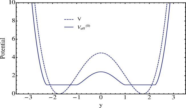
Figure 1: The dashed and solid curves show the double-well potential $V(y)=\frac{1}{2}(y^{2}-\mu^{2})^{2}$ and the effective potential $V_{\rm eff}^{(0)}(y)$ respectively for $\mu^{2}=3$.

For the $y$-integration in (3.12), we focus on a region near the origin that would be responsible for contributions from instantons, as discussed in [20]. For $|y|<a$, we find:

$$N\left(V_{\rm eff}^{(0)}(y)-1\right)=N\left[\frac{4}{3}\,(a^{2}-y^{2})^{3/2}+\frac{1}{10}\,(a^{2}-y^{2})^{5/2}+{\cal O}\left((a^{2}-y^{2})^{7/2}\right)\right],$$ (3.20)

where only the first term survives in the double scaling limit, and the integration near the origin leads to

$$\int_{0}2ydy\,e^{-N(V^{(0)}_{\rm eff}(y)-1)} = \int^{a^{2}}ds\,e^{-\frac{4}{3}\,Ns^{3/2}}=\frac{4t}{N^{2/3}}\int^{1}ds\,e^{-\frac{32}{3}\,t^{3/2}s^{3/2}}$$ (3.21)

$$= -\frac{1}{4N^{2/3}t^{1/2}}\,e^{-\frac{32}{3}\,t^{3/2}}\,\left(1+{\cal O}(t^{-3/2})\right)$$

for the case of $t$ finite but large. The exponent is nothing but the height of the potential barrier of $NV^{(0)}_{\rm eff}(y)$:

$$e^{-N(V_{\rm eff}^{(0)}(0)-1)}=e^{-\frac{32}{3}\,t^{3/2}}.$$ (3.22)

For the contribution from the potential at subleading order $V_{\rm eff}^{(1)}(y)$, we substitute it with the value at the origin $V_{\rm eff}^{(1)}(0)$. Then, the free energy (3.7) becomes

$$F_{(1,0)}=Ne^{-N}\left.Z^{\prime}_{(1,0)}\right|_{0{\rm-inst.}}\frac{e^{-V_{\rm eff}^{(1)}(0)}}{4N^{2/3}t^{1/2}}\,e^{-\frac{32}{3}\,t^{3/2}}\,\left(1+{\cal O}(t^{-3/2})\right)+\cdots.$$ (3.23)

Contribution from the remaining factors

Next, let us evaluate the contribution from the factor $\left.Z^{\prime}_{(1,0)}\right|_{0{\rm-inst.}}$ in (3.23). Taking

$$\lambda_{i}=\left(\frac{N-1}{N}\right)^{\frac{1}{4}}\lambda_{i}^{\prime},\quad\mu=\left(\frac{N-1}{N}\right)^{\frac{1}{4}}\mu^{\prime},\quad a=\left(\frac{N-1}{N}\right)^{\frac{1}{4}}a^{\prime},\quad b=\left(\frac{N-1}{N}\right)^{\frac{1}{4}}b^{\prime}\ ,$$ (3.24)

one finds

$$\left.Z^{\prime}_{(1,0)}\right|_{0{\rm-inst.}} = \frac{\tilde{C}_{N}}{\tilde{C}_{N-1}}\left(\frac{N-1}{N}\right)^{\frac{(N-1)^{2}}{2}}$$

$$\times\tilde{C}_{N-1}\int^{b^{\prime}}_{a^{\prime}}\prod_{i=1}^{N-1}(2\lambda_{i}^{\prime}d\lambda_{i}^{\prime})\left\{\prod_{N-1\geq i>j\geq 1}(\lambda_{i}^{\prime 2}-\lambda_{j}^{\prime 2})^{2}\right\}e^{-(N-1)\sum_{i=1}^{N-1}\frac{1}{2}(\lambda_{i}^{\prime 2}-\mu^{\prime 2})^{2}}.$$

Note that the last line in (LABEL:Z'0inst2) is nothing but $\left.Z_{(1,0)}\right|_{0{\rm-inst.}}$ with the replacements

$$N\to N-1,\qquad\mu\to\mu^{\prime},\qquad a\to a^{\prime},\qquad b\to b^{\prime}.$$ (3.26)

Therefore, the last line in (LABEL:Z'0inst2) equals unity by a perturbative argument around the saddle point $\lambda_{i}^{\prime}=\mu^{\prime}$ ($i=1,\cdots,N$) which is parallel to the derivation of (3.6), i.e. (A.7). By using (2.9), we obtain

$$\left.Z^{\prime}_{(1,0)}\right|_{0{\rm-inst.}}=\frac{\tilde{C}_{N}}{\tilde{C}_{N-1}}\left(\frac{N-1}{N}\right)^{\frac{(N-1)^{2}}{2}}=\frac{e^{N}}{2\pi N}\times\left(1+{\cal O}(N^{-1})\right).$$ (3.27)

Also, $V_{\rm eff}^{(1)}(0)$ is computed in appendix B, and the result (B.18) gives

$$e^{-V_{\rm eff}^{(1)}(0)}=\frac{N^{2/3}}{16t}\times\left(1+{\cal O}(N^{-1/3})\right).$$ (3.28)

Final result

Plugging (3.27) and (3.28) into (3.23), we see that the double scaling limit leaves a finite and nontrivial function of $t$:

$$F_{(1,0)}=\frac{1}{128\pi\,t^{3/2}}\,e^{-\frac{32}{3}t^{3/2}}\,\left(1+{\cal O}(t^{-3/2})\right)+(\mbox{multi-instantons})$$ (3.29)

for $t$ finite but large. The result supports the validity of taking (2.17) as a scaling variable. Similar to the $c=0$ case [20], it would be natural to regard instantons in the matrix model as kinds of D-branes in the corresponding type IIA superstring theory in two dimensions [11, 12]. In fact, $e^{-\frac{32}{3}t^{3/2}}$ is essentially the exponential series of the disk amplitude whose boundary is placed at the position of the instanton $y=0$: $\left.\left\langle 2{\rm Re}\,\sum_{i=1}^{N}\ln(y^{2}-\lambda_{i}^{2})\right\rangle_{\rm planar}^{(1,0)}\right|_{y=0}$, which seems parallel to the argument in [26]. The remaining factor $\frac{1}{128\pi\,t^{3/2}}$ in (3.29) receives contributions from fluctuation in the position of the instanton and from the exponential of the annulus amplitude at the origin: $\left.\frac{1}{2}\left\langle\left\{2{\rm Re}\,\sum_{i=1}^{N}\ln(y^{2}-\lambda_{i}^{2})\right\}^{2}\right\rangle_{C,\,{\rm planar}}^{\,(1,0)}\right|_{y=0}$. The difference of disk amplitudes $\Delta_{0}D(0)$ does not contribute in the double scaling limit as seen in appendix B. This would be clarified by considering analogs of FZZT or ZZ branes [27, 28, 29] in the type IIA superstring theory and computing amplitudes in the presence of such branes. We leave it as a future subject for investigation.

We also comment on two notable points which differ from the situation for the $c=0$ case. First, the instanton effect (3.29) is a real number, while it is pure imaginary in the $c=0$ case [20] indicating instability of that system. Technically, the result of the latter is attributed to rotating the integration path of an eigenvalue in order to obtain a finite result. Our computation does not need such a rotation of the integration path, and the result does not seem to exhibit any instability . This provides evidence that our matrix model leads to a sensible theory in the double scaling limit. Second, the powers of $N$ appearing in (3.29) are integers by recalling (2.17), while in the $c=0$ case [20] they are half-integers . Our result tempts us to interpret contributions to (3.29) as string worldsheets with holes at the positions of instantons based on the identification of $1/N$ as a string coupling. However, such an interpretation does not seem straightforward when considering contributions from the $y$-integral which represent the fluctuations in the position of the instanton.

4 Orthogonal polynomials

In sections 5 and 6, we compute nonperturbative effects including the result obtained in the previous section in a more efficient way. In preparation for this, let us first introduce orthogonal polynomials for the matrix model in this section.

Under the change of variables $x_{i}=\lambda_{i}^{2}-\mu^{2}$, the partition function $Z_{(1,0)}$ defined in (2.10) reduces to Gaussian matrix integrals

$$Z_{(1,0)}=\tilde{C}_{N}\int^{\infty}_{-\mu^{2}}\left(\prod_{i=1}^{N}dx_{i}\right)\,\triangle(x)^{2}\,e^{-N\sum_{i=1}^{N}\frac{1}{2}x_{i}^{2}}.$$ (4.1)

It seems almost trivial, but a nontrivial effect possibly arises from the boundary of the integration region. Ref. [25] mentions that the boundary effect is nonperturbative in $1/N$. Indeed, if we neglect it by replacing the lower bound $-\mu^{2}$ with $-\infty$, (4.1) will coincide with the perturbative result (2.16) or (3.6). This suggests that the supersymmetry is unbroken to all orders in the $1/N$ expansion.

Let us consider polynomials

$$P_{n}(x)=x^{n}+\sum_{i=0}^{n-1}p_{n}^{(i)}x^{i}\qquad(n=0,1,2,\cdots)$$ (4.2)

with the coefficient of the top degree ($x^{n}$) fixed to 1. The coefficients $p_{n}^{(i)}$ are uniquely determined so that the orthogonality relation

$$(P_{n},\,P_{m})\equiv\int^{\infty}_{-\mu^{2}}dx\,e^{-\frac{N}{2}x^{2}}\,P_{n}(x)\,P_{m}(x)=h_{n}\delta_{n,m}$$ (4.3)

is satisfied. Similar to the case without a boundary [32], we have recursion relations of the form

$$xP_{m}(x)=P_{m+1}(x)+S_{m}P_{m}(x)+R_{m}P_{m-1}(x),$$ (4.4)

$$h_{m}=R_{m}h_{m-1}.$$ (4.5)

For example, the first few quantities are

$$h_{0}=\sqrt{\frac{2\pi}{N}}\left[1-\frac{1}{2}\,\mbox{erfc}\left(\sqrt{\frac{N}{2}}\,\mu^{2}\right)\right],$$ (4.6)

$$S_{0}=-p_{1}^{(0)}=\frac{1}{Nh_{0}}\,e^{-\frac{N}{2}\mu^{4}},$$ (4.7)

$$h_{1}=\frac{1}{N}\,h_{0}-\frac{1}{N}\,\mu^{2}\,e^{-\frac{N}{2}\,\mu^{4}}-\frac{1}{N^{2}h_{0}}\,e^{-N\mu^{4}},$$ (4.8)

where

$$\mbox{erfc}(x)\equiv\frac{2}{\sqrt{\pi}}\int^{\infty}_{x}dt\,e^{-t^{2}}.$$ (4.9)

Then, (4.1) and the expectation value $\left\langle\frac{1}{N}{\rm tr}\,(\phi^{2}-\mu^{2})\right\rangle^{(1,0)}$ are expressed as

$$Z_{(1,0)}=\tilde{C}_{N}\,N!\left(\prod_{n=0}^{N-1}h_{n}\right)$$ (4.10)

and

$$\left\langle\frac{1}{N}{\rm tr}\,(\phi^{2}-\mu^{2})\right\rangle^{(1,0)} = \frac{1}{Z_{(1,0)}}\,\tilde{C}_{N}\int^{\infty}_{-\mu^{2}}\left(\prod_{i=1}^{N}dx_{i}\right)\,\triangle(x)^{2}\,e^{-N\sum_{i=1}^{N}\frac{1}{2}x_{i}^{2}}\,\frac{1}{N}\sum_{k=1}^{N}x_{k}$$ (4.11)

$$= \frac{1}{N}\sum_{n=0}^{N-1}S_{n},$$

respectively. We will compute (4.11) later by taking into account the boundary effect. The identities

$$\int^{\infty}_{-\mu^{2}}dx\,\frac{d}{dx}\left(e^{-\frac{N}{2}x^{2}}\,P_{n}(x)^{2}\right)=-e^{-\frac{N}{2}\mu^{4}}\,P_{n}(-\mu^{2})^{2},$$ (4.12)

$$\int^{\infty}_{-\mu^{2}}dx\,\frac{d}{dx}\left(e^{-\frac{N}{2}x^{2}}\,P_{n}(x)P_{n-1}(x)\right)=-e^{-\frac{N}{2}\mu^{4}}\,P_{n}(-\mu^{2})P_{n-1}(-\mu^{2})$$ (4.13)

lead to relations which include the boundary effects:

$$S_{n} = \frac{1}{N}\frac{1}{h_{n}}\,P_{n}(-\mu^{2})^{2}\,e^{-\frac{N}{2}\mu^{4}},$$ (4.14)

$$R_{n} = \frac{n}{N}+\frac{1}{N}\frac{1}{h_{n-1}}\,P_{n}(-\mu^{2})P_{n-1}(-\mu^{2})\,e^{-\frac{N}{2}\mu^{4}}.$$ (4.15)

As an approximation of the zeroth order contributions, let us simply neglect the boundary effect. This corresponds to changing the lower bound of the integral (4.3) to $-\infty$ and dropping terms containing $e^{-\frac{N}{2}\mu^{4}}$ in (4.14) and (4.15). The orthogonal polynomials in this case, denoted by $P^{(H)}_{n}(x)$, are given by the Hermite polynomials:

$$P^{(H)}_{n}(x)=\frac{1}{(2N)^{n/2}}\,H_{n}\left(\sqrt{\frac{N}{2}}\,x\right)$$ (4.16)

with

$$H_{n}(x)\equiv(-1)^{n}\,e^{x^{2}}\frac{d^{n}}{dx^{n}}\,e^{-x^{2}}$$ (4.17)

and coefficients

$$S_{n}^{(H)}=0,\qquad R^{(H)}_{n}=\frac{n}{N},\qquad h_{n}^{(H)}=\sqrt{2\pi}\,\frac{n!}{N^{n+\frac{1}{2}}}.$$ (4.18)

The superscript $(H)$ represents quantities in the zeroth order approximation.

We will compute corrections due to the boundary, denoted by quantities with tildes:

$$P_{n}(x)=P^{(H)}_{n}(x)+\tilde{P}_{n}(x),$$

$$S_{n}=S^{(H)}_{n}+\tilde{S}_{n},\qquad R_{n}=R^{(H)}_{n}+\tilde{R}_{n},\qquad h_{n}=h^{(H)}_{n}+\tilde{h}_{n}$$ (4.19)

in an iterative manner. In terms of the ratio

$$k_{m}(x)=\frac{P_{m}(x)}{P_{m-1}(x)},$$ (4.20)

(4.4) is expressed as

$$x=k_{m+1}(x)+S_{m}+\frac{R_{m}}{k_{m}(x)}.$$ (4.21)

The zeroth and first order contributions to (4.21) with respect to the corrections are

$$x=k^{(H)}_{m+1}(x)+\frac{m}{N}\,\frac{1}{k_{m}^{(H)}(x)}$$ (4.22)

and

$$0=k_{m+1}^{(H)}(x)\tilde{L}_{m+1}(x)-x\tilde{L}_{m}(x)+\frac{1}{k_{m}^{(H)}(x)}\frac{m}{N}\tilde{L}_{m-1}(x)+\tilde{S}_{m}+\frac{1}{k_{m}^{(H)}(x)}\tilde{R}_{m},$$ (4.23)

where

$$k^{(H)}_{m}(x)\equiv\frac{P^{(H)}_{m}(x)}{P^{(H)}_{m-1}(x)},\qquad\tilde{L}_{m}(x)\equiv\frac{\tilde{P}_{m}(x)}{P_{m}^{(H)}(x)}.$$ (4.24)

We expand quantities with tildes in terms of instanton number as:

$$\tilde{S}_{n} = \tilde{S}^{(1)}_{n}+\tilde{S}^{(2)}_{n}+\cdots,$$

$$\tilde{R}_{n} = \tilde{R}^{(1)}_{n}+\tilde{R}^{(2)}_{n}+\cdots,$$

$$\tilde{h}_{n} = \tilde{h}^{(1)}_{n}+\tilde{h}^{(2)}_{n}+\cdots,$$

$$\tilde{L}_{n}(x) = \tilde{L}^{(1)}_{n}(x)+\tilde{L}^{(2)}_{n}(x)+\cdots.$$ (4.25)

The superscripts $(1),(2),\cdots$ represent contributions from one instanton, two instantons and so forth.

5 One-instanton contribution

In this section, we consider (4.22) as the first iteration with respect to the instanton number. The obtained result is interpreted as a nonperturbative effect from a one-instanton configuration.

5.1 Leading order

Following the argument in section 3.2 of [20], we assume that $k^{(H)}_{m}(x)$ has smooth large-$N$ behavior given by

$$k^{(H)}_{m}(x)=k^{(0)}(x,\xi)+\frac{1}{N}\,k^{(1)}(x,\xi)+{\cal O}(N^{-2})$$ (5.1)

with $\xi=\frac{m}{N}$. Then, ${\cal O}(N^{0})$ and ${\cal O}(N^{-1})$ contributions to (4.22) determine $k^{(0)}(x,\xi)$ and $k^{(1)}(x,\xi)$ to be

$$k^{(0)}(x,\xi) = \mbox{sgn}(x)\frac{|x|+\sqrt{x^{2}-4\xi}}{2}\qquad\mbox{for}\qquad|x|>2,$$

$$k^{(1)}(x,\xi) = -\frac{1}{2}k^{(0)}(x,\xi)\partial_{\xi}\ln\sqrt{x^{2}-4\xi}.$$ (5.2)

The orthogonal polynomial $P^{(H)}_{n}(x)$ for $|x|>2$ can be expressed by

$$P^{(H)}_{n}(x) = \prod_{m=1}^{n}k^{(H)}_{m}(x)$$ (5.3)

$$= (\mbox{sgn}(x))^{n}\,\exp\left[\sum_{m=1}^{n}\ln|k^{(0)}(x,\xi)|+\frac{1}{N}\sum_{m=1}^{n}\frac{k^{(1)}(x,\xi)}{k^{(0)}(x,\xi)}+{\cal O}(N^{-1})\right],$$

where we consider $n$ running up to $N-1$. The Euler-Maclaurin formula

$$\sum_{m=1}^{n}f\left(\frac{m}{N}\right)=N\int^{\frac{n}{N}}_{\frac{1}{N}}d\xi\,f(\xi)+\frac{1}{2}\left\{f\left(\frac{1}{N}\right)+f\left(\frac{n}{N}\right)\right\}+{\cal O}(N^{-1})$$ (5.4)

converts the sums to integrals. After calculating the integrals, we end up with

$$P^{(H)}_{n}(x) = (\mbox{sgn}(x))^{n}\,\left(\frac{|x|+\sqrt{x^{2}-4\frac{n}{N}}}{2}\right)^{n+\frac{1}{2}}\frac{1}{(x^{2}-4\frac{n}{N})^{1/4}}$$ (5.5)

$$\times\exp\left[\frac{N}{4}x^{2}-\frac{N}{4}|x|\sqrt{x^{2}-4\frac{n}{N}}-\frac{1}{2}n+{\cal O}(N^{-1})\right]$$

for $|x|>2$.

By using (4.18) and (5.5), the leading contribution to the correction $\tilde{S}_{n}$ in (4.14):

$$\tilde{S}_{n}^{(1)} = \frac{1}{N}\frac{1}{h^{(H)}_{n}}\,P^{(H)}_{n}(-\mu^{2})^{2}\,e^{-\frac{N}{2}\mu^{4}}$$ (5.6)

can be expressed as

$$\tilde{S}_{n}^{(1)} = \frac{1}{\sqrt{2\pi}}\,\exp\Bigg{[}\left(n-\frac{1}{2}\right)\ln N-\ln n!+(2n+1)\ln\frac{\mu^{2}+\sqrt{\mu^{4}-4\frac{n}{N}}}{2}$$ (5.7)

$$\hskip 51.21495pt-\ln\sqrt{\mu^{4}-4\frac{n}{N}}-\frac{N}{2}\mu^{2}\sqrt{\mu^{4}-4\frac{n}{N}}-n\Bigg{]}\times\{1+{\cal O}(N^{-1})\}.$$

Let us consider the corresponding contribution to (4.11):

$$\left.\left\langle\frac{1}{N}{\rm tr}\,(\phi^{2}-\mu^{2})\right\rangle^{(1,0)}\right|_{\rm 1-inst.}=\frac{1}{N}\sum_{n=0}^{N-1}\tilde{S}^{(1)}_{n},$$ (5.8)

where the summand (5.7) near $n=N-1$ has the mildest damping in the exponent and gives a dominant effect, by noting

$$\sqrt{\mu^{4}-4\frac{n}{N}}=2\sqrt{\left(1-\frac{n}{N}\right)+4\omega+4\omega^{2}}$$ (5.9)

with $\omega$ small . Thus, we may consider contributions around the upper limit of the sum (5.8) and recast it as

$$\left.\left\langle\frac{1}{N}{\rm tr}\,(\phi^{2}-\mu^{2})\right\rangle^{(1,0)}\right|_{\rm 1-inst.}=\frac{1}{N}\frac{1}{2\pi}\int^{1-\frac{1}{N}}d\xi\,e^{Nf_{0}(\xi)+f_{1}(\xi)}\,\times[1+{\cal O}(N^{-1})]$$ (5.10)

with

$$f_{0}(\xi) \equiv -\xi\ln\xi+2\xi\ln\frac{\mu^{2}+\sqrt{\mu^{4}-4\xi}}{2}-\frac{1}{2}\mu^{2}\sqrt{\mu^{4}-4\xi},$$

$$f_{1}(\xi) \equiv -\frac{1}{2}\ln\xi+\ln\frac{\mu^{2}+\sqrt{\mu^{4}-4\xi}}{2}-\ln\sqrt{\mu^{4}-4\xi}.$$ (5.11)

We take $\xi=(1-\frac{1}{N})\xi^{\prime}$ and change the integration variable to $s=\sqrt{1-\frac{4\xi^{\prime}}{\mu^{4}}}$ to obtain

$$\left.\left\langle\frac{1}{N}{\rm tr}\,(\phi^{2}-\mu^{2})\right\rangle^{(1,0)}\right|_{\rm 1-inst.}=\frac{1}{N}\frac{-\mu^{2}}{4\pi}\,F\left(\sqrt{1-\frac{4}{\mu^{4}}}\right)\times[1+{\cal O}(N^{-1})],$$ (5.12)

where

$$F(\varepsilon) \equiv \int^{\varepsilon}ds\,\exp\left[N\mu^{4}\left\{\frac{1-s^{2}}{4}\ln\left(1+\frac{2s}{1-s}\right)-\frac{1}{2}s\right\}\right]$$ (5.13)

$$\hskip 22.76219pt\times\exp\left[-\frac{\mu^{4}(1-s^{2})-2}{4}\ln\left(1+\frac{2s}{1-s}\right)\right].$$

Because $\sqrt{1-\frac{4}{\mu^{4}}}=2\sqrt{\omega}\left[1-\frac{3}{2}\omega+{\cal O}(\omega^{2})\right]$ is a small quantity, let us consider $F(\varepsilon)$ for $\varepsilon$ small. When $N\varepsilon^{3}$ is kept finite but large as $N\sim\infty$ and $\varepsilon\sim 0$,

$$F(\varepsilon)=\int^{\varepsilon}ds\,e^{-N\mu^{4}\,\frac{s^{3}}{3}}\,(1+{\cal O}(s))=\frac{-1}{N\mu^{4}\varepsilon^{2}}\,e^{-N\mu^{4}\,\frac{\varepsilon^{3}}{3}}\,\left[1+{\cal O}\left(\frac{1}{N\varepsilon^{3}}\right)\right].$$ (5.14)

The expression on the r.h.s. is confirmed by taking a derivative with respect to $\varepsilon$. This gives the final result

$$\left.\left\langle\frac{1}{N}{\rm tr}\,(\phi^{2}-\mu^{2})\right\rangle^{(1,0)}\right|_{\rm 1-inst.}=N^{-4/3}\,\hat{\Omega}^{(1)}_{0}(t)\,\left[1+{\cal O}(t^{-3/2})\right]$$ (5.15)

with

$$\hat{\Omega}^{(1)}_{0}(t)\equiv\frac{1}{32\pi t}\,e^{-\frac{32}{3}\,t^{3/2}}$$ (5.16)

for $t$ fixed to be finite but large. From (2.15) and (5.15), we can conclude that the nonperturbative effect dynamically breaks the supersymmetry (under wave function renormalization absorbing the factor $N^{-4/3}$) .

The contribution to the free energy $F_{(1,0)}$ is obtained by integrating (2.14) as

$$\left.F_{(1,0)}\right|_{\rm 1-inst.} = 4\int^{\infty}_{t}dt^{\prime}\,\hat{\Omega}^{(1)}_{0}(t^{\prime})\,\left[1+{\cal O}(t^{\prime-3/2})\right]$$ (5.17)

$$= \frac{1}{128\pi\,t^{3/2}}\,e^{-\frac{32}{3}\,t^{3/2}}\,\left[1+{\cal O}(t^{-3/2})\right].$$

The integration constant is determined from the fact that there is no perturbative contribution to $F_{(1,0)}$, as seen from (2.16) or (3.6). Notice that (5.17) coincides with the result (3.29) not only in the exponential factor $e^{-\frac{32}{3}\,t^{3/2}}$ but also in the prefactor $\frac{1}{128\pi\,t^{3/2}}$. Moreover, the agreement of the exponential factors is already seen before taking the double scaling limit. Namely, $(V_{\rm eff}^{(0)}(0)-1)$ obtained from (3.19) is exactly equal to $-f_{0}(1)$ from (5.11). It gives additional grounds for regarding the results (5.15) and (5.17) as one-instanton contributions to $\left\langle\frac{1}{N}{\rm tr}\,(\phi^{2}-\mu^{2})\right\rangle^{(1,0)}$ and $F_{(1,0)}$, respectively. Thus (5.15) shows that the instanton induces the supersymmetry breaking.

5.2 Full one-instanton contribution

Here we compute the one-instanton effect to all orders, namely full contributions to the factors $[1+{\cal O}(t^{-3/2})]$ in (5.15) and (5.17).

Substituting (4.16), (4.18) and (5.6) in (5.8), we have

$$\left.\left\langle\frac{1}{N}{\rm tr}\,(\phi^{2}-\mu^{2})\right\rangle^{(1,0)}\right|_{\rm 1-inst.}=\frac{e^{-z^{2}}}{\sqrt{2\pi}\,N^{3/2}}\,\frac{1}{2^{N}\,(N-1)!}\,\left[H_{N}(z)^{2}-H_{N-1}(z)\,H_{N+1}(z)\right],$$ (5.18)

where

$$z\equiv\sqrt{\frac{N}{2}}\,\mu^{2}=\sqrt{2N}\,(1+2\omega),$$ (5.19)

and the relation

$$\sum_{k=0}^{n-1}\frac{1}{2^{k}k!}\,H_{k}(x)^{2}=\frac{1}{2^{n}\,(n-1)!}\left[H_{n}(x)^{2}-H_{n-1}(x)\,H_{n+1}(x)\right]$$ (5.20)

was used. The latter can be proved by an inductive argument. Upon taking the double scaling limit in (5.18), the following asymptotic formula plays a relevant role:

$$e^{-x^{2}/2}H_{n}(x)=\pi^{\frac{1}{4}}2^{\frac{n}{2}+\frac{1}{4}}n^{-\frac{1}{12}}\sqrt{n!}\left[{\rm Ai}(s)+n^{-2/3}g_{0}(s)+n^{-1}g_{1}(s)+\cdots\right]$$ (5.21)

which is valid for large $n$ with

$$x=\sqrt{2n+1}+\frac{s}{\sqrt{2}\,n^{1/6}}.$$ (5.22)

The Airy function is defined by

$${\rm Ai}(s)\equiv\frac{1}{2\pi}\int^{\infty}_{-\infty}dz\,e^{-isz-\frac{i}{3}z^{3}},$$ (5.23)

and $g_{0}(s),g_{1}(s),\cdots$ are functions depending only on $s$. The appearance of the Airy function in (5.21) seems reasonable from the WKB analysis of the harmonic oscillator potential around its turning points. See appendix C for a derivation of (5.21). In applying (5.21) to (5.18), notice that

$$s = 4t-\frac{1}{2}N^{-1/3}+\frac{1}{16}N^{-4/3}+{\cal O}(N^{-7/3})\qquad\mbox{for}\quad H_{N},$$

$$s = 4t+\frac{1}{2}N^{-1/3}-\frac{2}{3}N^{-1}t-\frac{1}{48}N^{-4/3}+{\cal O}(N^{-2})\qquad\mbox{for}\quad H_{N-1},$$

$$s = 4t-\frac{3}{2}N^{-1/3}+\frac{2}{3}N^{-1}t+\frac{5}{16}N^{-4/3}+{\cal O}(N^{-2})\qquad\mbox{for}\quad H_{N+1}.$$ (5.24)

We find that the full one-instanton contribution is given in terms of the Airy function and its derivative, by

$$\left.\left\langle\frac{1}{N}{\rm tr}\,(\phi^{2}-\mu^{2})\right\rangle^{(1,0)}\right|_{\rm 1-inst.}=N^{-4/3}\left[\Omega_{0}^{(1)}(t)+N^{-2/3}\,\Omega^{(1)}_{2/3}(t)+{\cal O}(N^{-1})\right],\\$$ (5.25)

with

$$\Omega_{0}^{(1)}(t)\equiv{\rm Ai}^{\prime}(4t)^{2}-4t{\rm Ai}(4t)^{2}$$ (5.26)

and corrections at order $N^{-2/3}$ nonvanishing. The subleading term

$$\Omega^{(1)}_{2/3}(t)=-\frac{12}{5}t^{2}{\rm Ai}(4t)^{2}+\frac{3}{20}\,{\rm Ai}(4t){\rm Ai}^{\prime}(4t)+\frac{2}{5}t\,{\rm Ai}^{\prime}(4t)^{2}$$ (5.27)

is obtained by using (C.16). From the asymptotic expansion of the Airy function:

$${\rm Ai}(s)=\frac{1}{2\pi}\frac{1}{s^{1/4}}\,e^{-\frac{2}{3}s^{3/2}}\sum_{n=0}^{\infty}\frac{\Gamma(\frac{1}{2}+3n)}{(2n)!}\left(-\frac{1}{9s^{3/2}}\right)^{n}$$ (5.28)

for large $s$, we see that all-order corrections to (5.16) take the form of

$$\Omega_{0}^{(1)}(t)=\frac{1}{32\pi t}\,e^{-\frac{32}{3}t^{3/2}}\,\left[1+\sum_{n=1}^{\infty}a^{(1)}_{n}\,\frac{1}{t^{\frac{3}{2}n}}\right]$$ (5.29)

with $a^{(1)}_{1}=-\frac{17}{192},\,a^{(1)}_{2}=\frac{1225}{73728},\,a^{(1)}_{3}=-\frac{199115}{42467328},\cdots$. The power series with respect to $t^{-3/2}$ can be regarded as perturbative contributions to all orders around the one-instanton configuration . Similar to (5.17), the full one-instanton contribution to the free energy $F_{(1,0)}$ gives

$$\left.F_{(1,0)}\right|_{\rm 1-inst.} = 4\int^{\infty}_{t}dt^{\prime}\,\Omega_{0}^{(1)}(t^{\prime})$$ (5.31)

$$= \frac{1}{3}\left[32t^{2}\,{\rm Ai}(4t)^{2}-{\rm Ai}(4t)\,{\rm Ai}^{\prime}(4t)-8t\,{\rm Ai}^{\prime}(4t)^{2}\right]$$

$$= \frac{1}{128\pi\,t^{3/2}}\,e^{-\frac{32}{3}\,t^{3/2}}\,\left[1+\sum_{n=1}^{\infty}b^{(1)}_{n}\,\frac{1}{t^{\frac{3}{2}n}}\right]$$ (5.32)

with $b^{(1)}_{1}=-\frac{35}{192},\,b^{(1)}_{2}=\frac{3745}{73728},\,b^{(1)}_{3}=-\frac{805805}{42467328},\cdots$.

Interestingly, (5.26) and (5.31) are closed form expressions and include fluctuations to all orders around the one-instanton configuration. The justification for this claim will become more evident in the next section, where we observe that all additional contributions to the one-point function and free energy involve only higher powers of $e^{-\frac{32}{3}\,t^{3/2}}$, and are thus attributed to $k$-instantons with $k>1$. It is an intriguing aspect of our supersymmetric matrix model, because in matrix models for bosonic strings such an expression has not been obtained even for the simplest case of $c=0$. It would be interesting to investigate the large order behavior of $a^{(1)}_{n}$ in (5.29) or $b^{(1)}_{n}$ in (5.32) and to compare the result with the large order growth $(2n)!$ in a string perturbation series [33]. Knowledge of this behavior could provide some insight into the stability of the one-instanton background.

6 Leading order two-instanton contribution

In this section, we calculate the leading order two-instanton contribution to the one-point function and free energy. For the effect on the one-point function (4.11), we need to know $\tilde{S}^{(2)}_{n}$.

6.1 Calculation of $\tilde{S}^{(2)}_{n}$

From (4.14), (4.19) and (5.6), one finds

$$\tilde{S}_{n}^{(2)}=\tilde{S}_{n}^{(1)}\left[-\frac{\tilde{h}_{n}^{(1)}}{h_{n}^{(H)}}+2\tilde{L}_{n}^{(1)}(-\mu^{2})\right].$$ (6.1)

In order to compute $\tilde{L}_{n}^{(1)}(-\mu^{2})$, we start from the first order expression for (4.23) obtained in an instanton number expansion:

$$-k_{m+1}^{(H)}(x)\,\tilde{L}^{(1)}_{m+1}(x)+x\tilde{L}^{(1)}_{m}(x)-\frac{\xi}{k_{m}^{(H)}(x)}\,\tilde{L}^{(1)}_{m-1}(x)=\left(1+\frac{\xi}{k_{m}^{(H)}(x)}\frac{1}{k^{(H)}_{m}(-\mu^{2})}\right)\tilde{S}^{(1)}_{m}\ ,$$ (6.2)

with $\xi=\frac{m}{N}$. Here,

$$\tilde{R}_{m}^{(1)}=\frac{1}{N}\frac{1}{h_{m-1}^{(H)}}P_{m}^{(H)}(-\mu^{2})P_{m-1}^{(H)}(-\mu^{2})\,e^{-\frac{N}{2}\mu^{4}}=\frac{\xi}{k_{m}^{(H)}(-\mu^{2})}\,\tilde{S}_{m}^{(1)}$$ (6.3)

was used. Since (6.3) can also be expressed as $k^{(H)}_{m}(-\mu^{2})\,\tilde{S}_{m-1}^{(1)}$, the relation

$$\tilde{S}^{(1)}_{m-1}=\frac{\xi}{k_{m}^{(H)}(-\mu^{2})^{2}}\,\tilde{S}_{m}^{(1)}$$ (6.4)

is obtained. For the leading order term in the two-instanton contribution, we may plug (5.1), (5.2) and

$$\tilde{S}_{m}^{(1)}=\frac{1}{2\pi}\frac{1}{N}\,e^{Nf_{0}(\xi)+f_{1}(\xi)}\,\times[1+{\cal O}(N^{-1})]$$ (6.5)

with (5.11) into the recursion relation (6.2). We find a solution for (6.2) by assuming the form of $\tilde{L}^{(1)}_{m}(x)$ as

$$\tilde{L}_{m}^{(1)}(x)=\left[L(x,\xi)+{\cal O}(N^{-1})\right]\tilde{S}_{m}^{(1)}.$$ (6.6)

Namely, $L(x,\xi)$ depends on $N$ only through $\xi$, and $\tilde{L}^{(1)}_{m}(x)$ and $\tilde{S}^{(1)}_{m}$ are of the same order in $1/N$.

By using (6.4), the recursion relation at leading order in $1/N$ becomes

$$\left[-k^{(0)}(x,\xi)\frac{1}{\xi}k^{(0)}(-\mu^{2},\xi)^{2}+x-\frac{1}{k^{(0)}(x,\xi)}\xi^{2}\frac{1}{k^{(0)}(-\mu^{2},\xi)^{2}}\right]L(x,\xi)$$

$$=1+\frac{1}{k^{(0)}(x,\xi)}\frac{\xi}{k^{(0)}(-\mu^{2},\xi)},$$ (6.7)

from which we have

$$L(x,\xi)=\frac{k^{(0)}(x,\xi)-k^{(0)}(-\mu^{2},\xi)-\mu^{2}}{xk^{(0)}(x,\xi)\left(2+\frac{\mu^{2}}{\xi}k^{(0)}(-\mu^{2},\xi)\right)-2\mu^{2}k^{(0)}(-\mu^{2},\xi)-\mu^{4}}.$$ (6.8)

This reduces to a simple formula at $x=-\mu^{2}$:

$$L(-\mu^{2},\xi)=\frac{\mu^{2}-\sqrt{\mu^{4}-4\xi}}{2(\mu^{4}-4\xi)},$$ (6.9)

and thus we obtain

$$\tilde{L}_{m}^{(1)}(-\mu^{2})=\left[\frac{\mu^{2}-\sqrt{\mu^{4}-4\frac{m}{N}}}{2(\mu^{4}-4\frac{m}{N})}+{\cal O}(N^{-1})\right]\,\tilde{S}_{m}^{(1)}\ .$$ (6.10)

Next, let us obtain $\tilde{h}_{n}^{(1)}$ in (6.1). From (4.19) one may rewrite $h_{n}=\left(\prod_{m=1}^{n}R_{m}\right)h_{0}$ as

$$h_{n} = \left(\prod_{m=1}^{n}R_{m}^{(H)}\right)\prod_{m=1}^{n}\left(1+\frac{\tilde{R}_{m}}{R_{m}^{(H)}}\right)\cdot h_{0}^{(H)}\left(1+\frac{\tilde{h}_{0}}{h_{0}^{(H)}}\right)$$ (6.11)

$$= h_{n}^{(H)}\left[1+\frac{\tilde{h}_{0}}{h_{0}^{(H)}}+\sum_{m=1}^{n}\frac{\tilde{R}^{(1)}_{m}}{R_{m}^{(H)}}+\mbox{(higher orders)}\right],$$

from which we read off

$$\frac{\tilde{h}_{n}^{(1)}}{h_{n}^{(H)}}=\frac{\tilde{h}_{0}}{h_{0}^{(H)}}+\sum_{m=1}^{n}\frac{N}{m}\,\tilde{R}^{(1)}_{m}.$$ (6.12)

Note that (4.6) and (4.18) allow us to express the first term in terms of the error function:

$$\frac{\tilde{h}_{0}}{h_{0}^{(H)}} = -\frac{1}{2}\,\mbox{erfc}\left(\sqrt{\frac{N}{2}}\mu^{2}\right)$$ (6.13)

$$= -\frac{1}{\sqrt{2\pi N}}\frac{1}{\mu^{2}}\,e^{-\frac{N}{2}\mu^{4}}\,[1+{\cal O}(N^{-1})].$$

Substituting (6.10) and (6.12) into (6.1), we have

$$\tilde{S}_{n}^{(2)} = \tilde{S}_{n}^{(1)}\frac{1}{2}\,\mbox{erfc}\left(\sqrt{\frac{N}{2}}\mu^{2}\right)$$ (6.14)

$$+\tilde{S}_{n}^{(1)}\sum_{m=1}^{n}\frac{\mu^{2}-\sqrt{\mu^{4}-4\frac{m}{N}}}{2\frac{m}{N}}\,\tilde{S}_{m}^{(1)}+\frac{\mu^{2}-\sqrt{\mu^{4}-4\frac{n}{N}}}{\mu^{4}-4\frac{n}{N}}\left(\tilde{S}^{(1)}_{n}\right)^{2}$$

after use of (6.3) and (6.13).

6.2 Calculation of nonperturbative effects

The sum $\frac{1}{N}\sum_{n=0}^{N-1}\tilde{S}^{(2)}_{n}$ gives the two-instanton contribution to $\left\langle\frac{1}{N}{\rm tr}\,(\phi^{2}-\mu^{2})\right\rangle^{(1,0)}$. The first term in the summand (6.14) is negligible at large $N$ due to the exponential damping in the error function. We therefore focus on the region $m\sim n\sim N-1$ in the sum of the second and third terms, which give relevant contributions.

The second term

Let us first consider the sum

$$\sum_{m=1}^{n}\frac{\mu^{2}-\sqrt{\mu^{4}-4\frac{m}{N}}}{2\frac{m}{N}}\,\tilde{S}_{m}^{(1)}$$ (6.15)

in the second term, focusing on the region $m=N-{\cal O}(N^{0})$, $n=N-{\cal O}(N^{0})$. Use of (6.5) gives

$$(\ref{2ndterm})=\frac{1}{2\pi}\int^{\xi}d\eta\,\frac{\mu^{2}-\sqrt{\mu^{4}-4\eta}}{2\eta}\,e^{Nf_{0}(\eta)+f_{1}(\eta)}\,\times\left[1+{\cal O}(N^{-1})\right].$$ (6.16)

Here, we take $\eta=\frac{m}{N}$ and $\xi=\frac{n}{N}$. We change the integration variable to $\eta=\xi\eta^{\prime}=\eta^{\prime}-(1-\xi)\eta^{\prime}$, and expand functions of $\eta^{\prime}-(1-\xi)\eta^{\prime}$ around $\eta^{\prime}$. By noting $1-\xi={\cal O}(N^{-1})$, we find

$$(\ref{2ndterm})=\frac{1}{2\pi}\int^{1}d\eta^{\prime}\,\frac{\mu^{2}-\sqrt{\mu^{4}-4\eta^{\prime}}}{2\eta^{\prime}\sqrt{\mu^{4}-4\eta^{\prime}}}\,e^{Nf_{0}(\eta^{\prime})+\tilde{f}_{1}(\eta^{\prime})}\times[1+{\cal O}(N^{-1})],$$ (6.17)

where

$$\tilde{f}_{1}(\eta^{\prime})\equiv\left(N(1-\xi)\eta^{\prime}-\frac{1}{2}\right)\left\{\ln\eta^{\prime}-2\ln\frac{\mu^{2}+\sqrt{\mu^{4}-4\eta^{\prime}}}{2}\right\}.$$ (6.18)

Next, the variable change $s=\sqrt{1-\frac{4\eta^{\prime}}{\mu^{4}}}$ leads to

$$(\ref{2ndterm})=\frac{-1}{2\pi}F_{1}\left(\sqrt{1-\frac{4}{\mu^{4}}}\right)\,\times[1+{\cal O}(N^{-1})]$$ (6.19)

with

$$F_{1}(\varepsilon) \equiv \int^{\varepsilon}\frac{ds}{1+s}\,\exp\left[N\mu^{4}\left\{\frac{1-s^{2}}{4}\ln\left(1+\frac{2s}{1-s}\right)-\frac{1}{2}s\right\}\right]$$ (6.20)

$$\times\exp\left[-\left\{N(1-\xi)\frac{\mu^{4}}{4}(1-s^{2})-\frac{1}{2}\right\}\ln\left(1+\frac{2s}{1-s}\right)\right].$$

Similar to (5.14),

$$F_{1}(\varepsilon)=\int^{\varepsilon}ds\,e^{-N\mu^{4}\frac{s^{3}}{3}}\,(1+{\cal O}(s))=\frac{-1}{N\mu^{4}\varepsilon^{2}}\,e^{-N\mu^{4}\frac{\varepsilon^{3}}{3}}\,\left[1+{\cal O}\left(\frac{1}{N\varepsilon^{3}}\right)\right]$$ (6.21)

is obtained for $N\varepsilon^{3}$ finite but large. Using this result gives

$$(\ref{2ndterm})=N^{-1/3}\,\frac{1}{32\pi t}\,e^{-\frac{32}{3}\,t^{3/2}}\,\left[1+{\cal O}(t^{-3/2})\right].$$ (6.22)

Since the $\xi$-dependent part does not contribute to (6.22), the summation of the second term in (6.14) with respect to $n$ reduces to $\frac{1}{N}\sum_{n=0}^{N-1}\tilde{S}_{n}^{(1)}$, which is nothing but (5.15). Thus we arrive at

$$\frac{1}{N}\sum_{n=0}^{N-1}\tilde{S}_{n}^{(1)}\sum_{m=1}^{n}\frac{\mu^{2}-\sqrt{\mu^{4}-4\frac{m}{N}}}{2\frac{m}{N}}\,\tilde{S}_{m}^{(1)}=N^{-5/3}\left(\frac{1}{32\pi t}\right)^{2}\,e^{-\frac{64}{3}\,t^{3/2}}\,\left[1+{\cal O}(t^{-3/2})\right].$$ (6.23)

The third term

The sum of the third term

$$\frac{1}{N}\sum_{n=0}^{N-1}\frac{\mu^{2}-\sqrt{\mu^{4}-4\frac{n}{N}}}{\mu^{4}-4\frac{n}{N}}\left(\tilde{S}^{(1)}_{n}\right)^{2}$$ (6.24)

can be evaluated in a similar manner. We convert the summation to an integral by taking $\xi=\frac{n}{N}$ as $\frac{1}{N}\sum_{n=0}^{N-1}\to\int^{1-\frac{1}{N}}d\xi$, and change the variable to $\xi=(1-\frac{1}{N})\xi^{\prime}$. This is then followed by a further variable change $s=\sqrt{1-\frac{4\xi^{\prime}}{\mu^{4}}}$. The result is

$$(\ref{sum_3rdterm})=\frac{-1}{8\pi^{2}}\frac{1}{N^{2}\mu^{2}}F_{2}\left(\sqrt{1-\frac{4}{\mu^{4}}}\right)\,\times[1+{\cal O}(N^{-1})]$$ (6.25)

with

$$F_{2}(\varepsilon) \equiv \int^{\varepsilon}ds\,\frac{1-s}{s^{3}}\,\exp\left[N\mu^{4}\left\{\frac{1-s^{2}}{2}\ln\left(1+\frac{2s}{1-s}\right)-s\right\}\right]$$ (6.26)

$$\hskip 54.06023pt\times\exp\left[-\left\{\frac{\mu^{4}}{2}(1-s^{2})-1\right\}\ln\left(1+\frac{2s}{1-s}\right)\right].$$

When $N\varepsilon^{3}$ is finite but large, $F_{2}(\varepsilon)$ can be evaluated as

$$F_{2}(\varepsilon)=\frac{-1}{2N\mu^{4}\varepsilon^{5}}\,e^{-2N\mu^{4}\frac{\varepsilon^{3}}{3}}\,\left[1+{\cal O}\left(\frac{1}{N\varepsilon^{3}}\right)\right],$$ (6.27)

leading to the result

$$\frac{1}{N}\sum_{n=0}^{N-1}\frac{\mu^{2}-\sqrt{\mu^{4}-4\frac{n}{N}}}{\mu^{4}-4\frac{n}{N}}\left(\tilde{S}^{(1)}_{n}\right)^{2}=N^{-4/3}\,\frac{1}{(64\pi)^{2}\,t^{5/2}}\,e^{-\frac{64}{3}\,t^{3/2}}\,\left[1+{\cal O}(t^{-3/2})\right].$$ (6.28)

Final result

Comparing the powers of $N$ between (6.23) and (6.28), we find that the latter is dominant. Thus, the two-instanton contribution is found to be

$$\left.\left\langle\frac{1}{N}{\rm tr}\,(\phi^{2}-\mu^{2})\right\rangle^{(1,0)}\right|_{\rm 2-inst.}=\frac{1}{N}\sum_{n=0}^{N-1}\tilde{S}_{n}^{(2)}=N^{-4/3}\,\hat{\Omega}^{(2)}_{0}(t)\,\left[1+{\cal O}(t^{-3/2})\right]$$ (6.29)

with

$$\hat{\Omega}^{(2)}_{0}(t)\equiv\frac{1}{(64\pi)^{2}\,t^{5/2}}\,e^{-\frac{64}{3}\,t^{3/2}},$$ (6.30)

for $t$ finite but large. Both effects from one instanton (5.15) and from two instantons (6.29) are of the same order in $N$ and equally contribute in the double scaling limit to the quantity

$$N^{4/3}\,\left\langle\frac{1}{N}{\rm tr}\,(\phi^{2}-\mu^{2})\right\rangle^{(1,0)}=N^{4/3}\,\frac{1}{N}\sum_{n=0}^{N-1}\left\{\tilde{S}_{n}^{(1)}+\tilde{S}_{n}^{(2)}+\cdots\right\}.$$ (6.31)

The weight of the exponential in (6.30) is twice that of (5.16), as it should be from the interpretation of a two-instanton contribution. In general, $\Omega^{(k)}_{0}(t)$ denotes the double scaling limit of $N^{4/3}\,\frac{1}{N}\sum_{n=0}^{N-1}\tilde{S}^{(k)}_{n}$ and $\hat{\Omega}_{0}^{(k)}(t)$ its leading large-$t$ behavior; these are both expected to give $k$-instanton contributions scaling as $e^{-\frac{32k}{3}\,t^{3/2}}$. Notice that we do not use the dilute gas approximation for instantons in this calculation. Namely, interactions among instantons are taken into account.

Correspondingly, the free energy is expressed as

$$F_{(1,0)}=\left.F_{(1,0)}\right|_{\rm 1-inst.}+\left.F_{(1,0)}\right|_{\rm 2-inst.}+\cdots,$$ (6.32)

where the first term is the one-instanton contribution given by (5.31) or (5.32), and the second term is

$$\left.F_{(1,0)}\right|_{\rm 2-inst.}=\frac{1}{2}\frac{1}{(128\pi)^{2}\,t^{3}}\,e^{-\frac{64}{3}\,t^{3/2}}\,\left[1+{\cal O}(t^{-3/2})\right]$$ (6.33)

due to two instantons. Since the dilute gas approximation does not give rise to multi-instanton contributions to the free energy , the result (6.33) is considered to be attributed solely to interactions between the instantons.

Since the contribution from each instanton sector is expected to be equally important in the double scaling limit, it would be nontrivial whether the full result including all instanton contributions gives a well-defined quantity or not, in particular for small $t$. In the next section, we will see numerical evidence suggesting that it is indeed well-defined.

7 Numerical result for full nonperturbative effects

In this section, we numerically compute the expectation value $\left\langle\frac{1}{N}{\rm tr}\,(\phi^{2}-\mu^{2})\right\rangle^{(1,0)}$ and the free energy $F_{(1,0)}$ including full nonperturbative effects. Starting with $P_{0}(-\mu^{2})=1$ and the expressions for $h_{0}$ and $S_{0}$ in (4.6) and (4.7) for a given value of $N$, we can carry out the following iterative procedure, beginning from $n=1$:

1. Evaluate $P_{n}(-\mu^{2})$ from (4.4).

2. Evaluate $R_{n}$ from (4.15).

3. Evaluate $h_{n}$ from (4.5).

4. Evaluate $S_{n}$ from (4.14).

5. Go back to 1. with $n$ incremented by one.

This procedure is repeated $N-1$ times to evaluate the values for $S_{n}$ ($n=1,\cdots,N-1$). The resulting $S_{n}$ are then combined with (4.11) to determine the exact one-point function for a given $N$ and $t$.

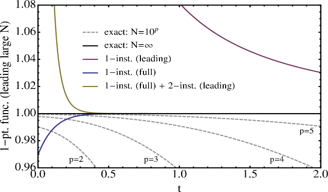
Figure 2: $\Omega(N,t)$ defined by (7.1) as a function of $t$. Everything is normalized by the $N=\infty$ result $\Omega_{0}(t)\equiv\Omega(\infty,t)$ (exact: $N=\infty$), and thus the black solid line representing it is flat. The gray dashed lines (exact: $N=10^{p}$) show the results $\Omega(N,t)$ for $N=10^{p}$ ($p=2,3,4,5$). The red line (1-inst. (leading)) and the blue line (1-inst. (full)) show the behavior of the leading one-instanton contribution $\hat{\Omega}^{(1)}_{0}(t)$ in (5.16) and the full one-instanton contribution $\Omega_{0}^{(1)}(t)$ in (5.26), respectively. Finally, the yellow line (1-inst. (full) + 2-inst. (leading)) represents the sum of the full one-instanton result $\Omega_{0}^{(1)}(t)$ and the leading two-instanton result $\hat{\Omega}^{(2)}_{0}(t)$ in (6.30).

We evaluate the one-point function

$$\Omega(N,t)\equiv N^{4/3}\left\langle\frac{1}{N}{\rm tr}\,(\phi^{2}-\mu^{2})\right\rangle^{(1,0)}$$ (7.1)

from $N=1$ to $N=1,000,000$, and then extrapolate the results to $N=\infty$ to obtain $\Omega_{0}(t)\equiv\Omega(\infty,t)$. The systematic error in the extrapolation is expected to be too small (around $10^{-7}\%$) to resolve in the presented figures. Fig. 2 summarizes our result for the one-point function. Everything in the plot is normalized by the $N=\infty$ result $\Omega_{0}(t)$, and we can see how finite $N$ results depicted by the gray dashed lines converge to the $N=\infty$ one. The result suggests that $t$ in (2.17) is the appropriate scaling variable in the double scaling limit. If this were not the case, $\Omega_{0}(t)$ would be driven to zero or infinity, and consequently all the gray dashed lines would lie at infinity or zero. Then, we could not obtain a sensible result such as in Fig. 2. The analytical results obtained in the previous sections are also plotted with this normalization. The full one-instanton result (5.26) significantly improves the approximation compared with the leading result (5.16). Although it is not clear in this figure whether or not the leading two-instanton contribution (6.30) makes the situation better, magnifying the neighborhood of 1.00 along the vertical axis as in Fig. 3 shows that it is indeed the case for $t\gtrsim 0.65$.

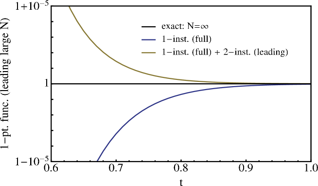
Figure 3: A magnified view of Fig. 2 around 1.00 in the vertical axis. Finite $N$ results lie outside the plot range.

We also find that the subleading correction with respect to $1/N$ (5.27) has good agreement with the corresponding numerical result, which is obtained from the subleading extrapolation parameters in $1/N$. For readers who have an interest, we present the result in Fig. 5 of appendix D.

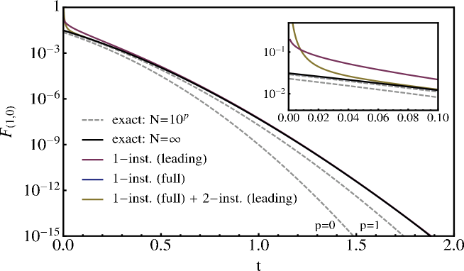
Figure 4: Full nonperturbative contribution to the free energy $F_{(1,0)}$ as a function of $t$. The black solid line (exact: $N=\infty$) represents the result of (7.2). For comparison, finite $N$ results ($4\int^{\infty}_{t}dt^{\prime}\,\Omega(N,t^{\prime})$ for various $N$) are shown by the gray dashed lines (exact: $N=10^{p}$). Also, the leading and full one-instanton contributions to $F_{(1,0)}$ (5.17) and (5.31) are depicted by the red and blue lines, respectively. The yellow line represents the sum of the full one-instanton result (5.31) and the leading two-instanton result in (6.33).

Finally we present in Fig. 4 the full nonperturbative contribution to the free energy $F_{(1,0)}=-\ln Z_{(1,0)}$ obtained by numerically integrating the $N=\infty$ result for the one-point function:

$$F_{(1,0)}=4\int^{\infty}_{t}dt^{\prime}\,\Omega_{0}(t^{\prime}).$$ (7.2)

Note that the free energy is a finite function of $t$ even at the origin, which corresponds to the strongly coupled limit of the type IIA superstring theory. In this limit, an approximation by the instanton number expansion does not make sense any longer. Instead there might be an appropriate description by weakly coupled degrees of freedom in an S-dual to the original theory. The behavior of the free energy might suggest the existence of such degrees of freedom.

From the viewpoint of perturbation theory, the free energy is expected to be formally expressed as a double series with respect to $t^{-3/2}$ and $e^{-\frac{32}{3}\,t^{3/2}}$ (the so-called trans-series [34]):

$$F_{(1,0)}=\sum_{k=1}^{\infty}e^{-\frac{32k}{3}\,t^{3/2}}\sum_{n=k}^{\infty}f^{(k)}_{n}\,t^{-\frac{3}{2}n}$$ (7.3)

with coefficients $f_{n}^{(k)}$. In matrix models for bosonic strings, it is extremely nontrivial to sum up such double series and obtain a well-defined result (for example, see [34, 35, 36]). However, in our matrix model for the IIA superstring theory, Fig. 4 indicates a well-defined result after we manage the summation.

8 Discussions

In this paper, we explicitly computed nonperturbative effects in a supersymmetric double-well matrix model [11] in the double scaling limit with $t=N^{2/3}\omega$ fixed. As was discussed in [11, 12], this model corresponds to type IIA superstring theory on a nontrivial Ramond-Ramond background in the two-dimensional target space (Liouville direction) $\times$ ($S^{1}$ with self-dual radius).

For the one-point function $\left\langle\frac{1}{N}{\rm tr}\,(\phi^{2}-\mu^{2})\right\rangle^{(1,0)}$ and the free energy $F_{(1,0)}$, full one-instanton contributions were obtained as closed form expressions containing all perturbative fluctuations around the one-instanton background. Also, presented were their analytic expressions for the leading two-instanton effect with respect to finite but large $t$. The result shows that the supersymmetry is spontaneously broken by nonperturbative effects due to instantons. In particular, the instanton effects survive in the double scaling limit, which implies that supersymmetry breaking takes place by nonperturbative dynamics in the target space of the type IIA superstring theory.

Moreover, we numerically evaluated full nonperturbative contributions to the one-point function and the free energy up to $N=1,000,000$, and extrapolated the results to $N=\infty$ in the double scaling limit. From the result, we further confirmed that $t$ is the correct scaling variable to be fixed in the double scaling limit. It was shown that the full one-instanton contribution to the one-point function gives a significantly better approximation of the $N=\infty$ result compared to the leading term in the one-instanton contribution, and that the leading two-instanton contribution further improves the result for $t\gtrsim 0.65$. The full nonperturbative free energy seems to be a finite function of $t$ even at the origin, which corresponds to the strongly coupled limit of the type IIA superstring theory. The result might suggest a well-defined weakly coupled theory as an S-dual to the IIA theory. It would be intriguing to obtain an analytic expression for the full nonperturbative contribution and to identify the S-dual theory.

In order to identify the Nambu-Goldstone fermions associated with the spontaneous supersymmetry breaking, let us express the auxiliary field $B_{ij}$ by its expectation value

$$\left\langle B_{ij}\right\rangle^{(1,0)}=-i\left\langle(\phi^{2}-\mu^{2})_{ij}\right\rangle^{(1,0)}=-i\left\langle\frac{1}{N}\,{\rm tr}(\phi^{2}-\mu^{2})\right\rangle^{(1,0)}\!\delta_{ij}$$ (8.1)

and fluctuations around it $\tilde{B}_{ij}$. The last equality comes from $U(N)$ symmetry of the system. Then, (2.5) leads to a nonlinear transformation:

$$Q\bar{\psi}_{ij}=-\left\langle\frac{1}{N}\,{\rm tr}(\phi^{2}-\mu^{2})\right\rangle^{(1,0)}\!\delta_{ij}-i\tilde{B}_{ij},$$ (8.2)

which is a signal of Nambu-Goldstone fermions according to the standard argument. Since the nonlinear term can be removed from $N-1$ of the $N$ independent components $\bar{\psi}_{ii}$ ($i=1,\cdots,N$) by taking appropriate linear combinations (for example, $\bar{\psi}_{11}-\bar{\psi}_{ii}$ ($i=2,\cdots,N$)), the linearly independent component $\frac{1}{N}\,{\rm tr}\,\bar{\psi}$ can be regarded as the Nambu-Goldstone fermion associated with the breaking of $Q$. Similarly, $\frac{1}{N}\,{\rm tr}\,\psi$ can be regarded as the Nambu-Goldstone fermion associated with the breaking of $\bar{Q}$. According to [11, 12], these correspond to (R$+$, NS) and (NS, R$-$) vertex operators in the type IIA theory:

$$\int d^{2}z\,V_{+\frac{1}{2},\,+1}(z)\,\bar{T}_{\frac{1}{2}}(\bar{z})=\int d^{2}z\,e^{-\frac{1}{2}\phi+\frac{i}{2}H+\frac{i}{2}x+\frac{1}{2}\varphi}(z)\,e^{-\bar{\phi}+\frac{i}{2}\bar{x}+\frac{1}{2}\bar{\varphi}}(\bar{z})$$ (8.3)

and

$$\int d^{2}z\,T_{-\frac{1}{2}}(z)\,\bar{V}_{-\frac{1}{2},\,-1}(\bar{z})=\int d^{2}z\,e^{-\phi-\frac{i}{2}x+\frac{1}{2}\varphi}(z)\,e^{-\frac{1}{2}\bar{\phi}-\frac{i}{2}\bar{H}-\frac{i}{2}\bar{x}+\frac{1}{2}\bar{\varphi}}(\bar{z})$$ (8.4)

(up to cocycle factors), respectively. Note that the Nambu-Goldstone fermions are generally not identical to fermion zero-modes in an instanton background. Suppose that diagonalization of $\phi$: $\phi=U\,{\rm diag}(\lambda_{1},\cdots,\lambda_{N})\,U^{\dagger}$ ($U\in SU(N)$) is accompanied with transformations of the fermions: $\psi=U\psi^{\prime}U^{\dagger}$ and $\bar{\psi}=U\bar{\psi}^{\prime}U^{\dagger}$. As discussed in section 3, one of the eigenvalues, say $y=\lambda_{N}$, sitting at the origin gives a configuration of a single instanton. Then, the fermionic variables $\psi^{\prime}_{NN}$ and $\bar{\psi}^{\prime}_{NN}$ will disappear from the classical action (2.1), becoming fermion zero-modes. Likewise, for a $k$-instanton configuration in which $\lambda_{j}$ ($j=N-k+1,\cdots,N$) are at the origin, $2k^{2}$ fermionic variables $\psi^{\prime}_{ij}$, $\bar{\psi}^{\prime}_{ij}$ ($i,j=N-k+1,\cdots,N$) will become zero-modes. Almost all of these zero-modes would be lifted by quantum effects due to the Vandermonde determinant. It would be interesting to consider a relation between the Nambu-Goldstone fermions and the fermion zero-modes. The fermion zero-modes might suggest that each eigenvalue at the origin corresponds to an object like a D-brane and anti-D-brane pair in the type IIA theory. This would be clarified by considering analogs of FZZT or ZZ branes [27, 28, 29] in the IIA superstring theory.

It would be interesting to consider various interpretations of the matrix variables in the matrix model. For instance, each matrix element could be regarded as a kind of string bit carrying a unit of winding or momentum along the $S^{1}$ target space, which seems to have some similarity to the matrix string theory [37]. Alternatively, the matrix elements might be interpreted as open string excitations on certain D-branes and the matrix model could describe closed string dynamics via the open-closed string duality [4, 5, 6, 8, 9, 10]. Refs. [38, 39, 40, 41] would be useful for furthering an investigation along these lines.

Note added

After this paper appeared in the arXiv, we were informed by Ricardo Schiappa that refs. [44, 45, 46] generalize the method of [20, 21] to be valid both in the double scaling limit and off-criticality. He also pointed out that trans-series and resurgent analysis discussed in [47, 48, 46] would be useful to compute higher instanton contributions in (7.3). Mithat Ünsal informed us of trans-series and resurgence approach to nonperturbative completion of quantum field theory (for example, see [49, 50, 51, 52]).

Appendix A Perturbative contributions to $Z_{(1,0)}$

In this appendix, we compute perturbative contributions to $Z_{(1,0)}$ by using a deformation method in topological field theory. Although related calculations are given in [22], we present a direct derivation here. First, $Z_{(1,0)}$ in (2.10) can be expressed in a form that involves the original matrix integrals:

$$Z_{(1,0)}=\left(-1\right)^{N^{2}}\int d^{N^{2}}B\int_{H_{+}}d^{N^{2}}\phi\int\left(d^{N^{2}}\psi\,d^{N^{2}}\bar{\psi}\right)\,e^{-S},$$ (A.1)

with $S$ given by (2.1). The integration region of $\phi$ is the space of positive definite Hermitian matrices $H_{+}$. We expand $\phi$ around the minimum $\mu$ of the double-well:

$$\phi=\mu+\tilde{\phi},$$ (A.2)

and compute $Z_{(1,0)}$ in perturbation theory with respect to small fluctuations $\tilde{\phi}$. The perturbative contribution can be expressed as

$$\left.Z_{(1,0)}\right|_{\rm pert.}\equiv\left(-1\right)^{N^{2}}\int d^{N^{2}}B\,d^{N^{2}}\tilde{\phi}\,\left(d^{N^{2}}\psi\,d^{N^{2}}\bar{\psi}\right)\,e^{-S_{\rm free}}\,\left[e^{-S_{\rm int.}}\right]_{\rm pert.},$$ (A.3)

where

$$S_{\rm free}\equiv N\,{\rm tr}\left[\frac{1}{2}B^{2}+i2\mu B\tilde{\phi}+2\mu\bar{\psi}\psi\right],\qquad S_{\rm int.}\equiv N\,{\rm tr}\left[iB\tilde{\phi}^{2}+\bar{\psi}\left(\tilde{\phi}\psi+\psi\tilde{\phi}\right)\right],$$ (A.4)

and the last factor $\left[e^{-S_{\rm int.}}\right]_{\rm pert.}$ means that the interaction part $S_{\rm int.}$ is treated in perturbation theory by expanding the exponential. Note that $\tilde{\phi}$ is integrated over all Hermitian matrices, following the conventional approach for perturbation theory around a saddle point of the classical action.

Since the integrand of (A.3) is invariant under the supersymmetry transformations (2.5) and (2.6) with the trivial change of $\phi$ to $\tilde{\phi}$, adding the term $N\,{\rm tr}\,(\frac{\epsilon-1}{2}B^{2})$ to the free part $S_{\rm free}$ does not affect the value of $\left.Z_{(1,0)}\right|_{\rm pert.}$ so long as the parameter $\epsilon$ is positive. For $\left.Z_{(1,0)}\right|_{\rm pert.}(\epsilon)$ denoting the deformed partition function, one can show

$$\frac{d}{d\epsilon}\left.Z_{(1,0)}\right|_{\rm pert.}(\epsilon)=0$$ (A.5)

for arbitrary positive $\epsilon$, from the facts that $N\,{\rm tr}\,(\frac{\epsilon-1}{2}B^{2})$ can be written in a $Q$-exact or $\bar{Q}$-exact form and that the deformation with $\epsilon>0$ does not change the asymptotic behavior of the integrand [42]. Rescaling $B\to\frac{1}{\sqrt{\epsilon}}\,B$ and $\tilde{\phi}\to\sqrt{\epsilon}\,\tilde{\phi}$ after the deformation, we find the expression:

$$\left.Z_{(1,0)}\right|_{\rm pert.}=\left(-1\right)^{N^{2}}\int d^{N^{2}}B\,d^{N^{2}}\tilde{\phi}\,\left(d^{N^{2}}\psi\,d^{N^{2}}\bar{\psi}\right)\,e^{-S_{\rm free}}\,\left[e^{-\sqrt{\epsilon}\,S_{\rm int.}}\right]_{\rm pert.}.$$ (A.6)

Because the value of $\left.Z_{(1,0)}\right|_{\rm pert.}$ does not depend on $\epsilon$, we may compute (A.6) in the limit $\epsilon\to+0$. Then, the matrix integral reduces to trivial Gaussian integrations. By using (2.3) and (2.4), it is easy to obtain

$$\left.Z_{(1,0)}\right|_{\rm pert.}=1.$$ (A.7)

This result is valid for arbitrary $N$.

Appendix B Computation of $V_{\rm eff}^{(1)}(0)$

In this appendix, we compute the value at $y=0$ of the effective potential at the subleading order $V_{\rm eff}^{(1)}(y)$ in (3.14).

B.1 Computation of $\Delta_{0}D(y^{2})$

Let us first evaluate the contribution from the difference of disk amplitudes $\Delta_{0}D(y^{2})$ defined by (3.11). After the same replacement as (3.24), $\left\langle\frac{1}{N}\sum_{i=1}^{N-1}\frac{1}{z-\lambda_{i}^{2}}\right\rangle_{\rm planar}^{{}^{\prime}\,(1,0)}$ becomes

$$\sqrt{\frac{N-1}{N}}\,\cdot\left.\left\langle\frac{1}{N}\sum_{i=1}^{N}\frac{1}{z-\lambda_{i}^{2}}\right\rangle_{\rm planar}^{(1,0)}\right|_{(N,\,\lambda_{i},\,z,\,\mu)\to(N-1,\,\lambda^{\prime}_{i},\,z^{\prime},\,\mu^{\prime})},$$ (B.1)

where $z=\left(\frac{N-1}{N}\right)^{\frac{1}{2}}z^{\prime}$. (3.15) gives the last factor of (B.1) as 

$$\frac{1}{2}\left[z^{\prime}-\mu^{\prime 2}-\sqrt{(z^{\prime}-\mu^{\prime 2})^{2}-4}\right].$$ (B.2)

Then,

$$\left\langle\frac{1}{N}\sum_{i=1}^{N-1}\frac{1}{z-\lambda_{i}^{2}}\right\rangle_{\rm planar}^{{}^{\prime}\,(1,0)} = \sqrt{\frac{N-1}{N}}\,\frac{1}{2}\left[z^{\prime}-\mu^{\prime 2}-\sqrt{(z^{\prime}-\mu^{\prime 2})^{2}-4}\right]$$

$$= \frac{1}{2}\left[z-\mu^{2}-\sqrt{(z-\mu^{2})^{2}-4\frac{N-1}{N}}\right]$$

$$= \left\langle\frac{1}{N}\sum_{i=1}^{N}\frac{1}{z-\lambda_{i}^{2}}\right\rangle^{(1,0)}_{\rm planar}-\frac{1}{N}\frac{1}{\sqrt{(z-a^{2})(z-b^{2})}}+{\cal O}(N^{-2}).$$

Similar to (3.16),

$$\left\langle\frac{1}{N}\sum_{i=1}^{N-1}\ln(y^{2}-\lambda_{i}^{2})\right\rangle_{\rm planar}^{{}^{\prime}\,(1,0)}=\lim_{\Lambda\to\infty}\left[\int^{y^{2}}_{\Lambda}dz\left\langle\frac{1}{N}\sum_{i=1}^{N-1}\frac{1}{z-\lambda_{i}^{2}}\right\rangle^{{}^{\prime}\,(1,0)}_{\rm planar}+\frac{N-1}{N}\ln\Lambda\right].$$ (B.4)

Plugging (LABEL:deltaD_1) into (B.4), we have

$$\Delta_{0}D(y^{2})=-2\lim_{\Lambda\to\infty}\left[{\rm Re}\int^{y^{2}}_{\Lambda}dz\frac{1}{\sqrt{(z-a^{2})(z-b^{2})}}+\ln\Lambda\right],$$ (B.5)

whose value at the origin is computed as

$$\Delta_{0}D(0) = 2\lim_{\Lambda\to\infty}\left[\int^{\Lambda}_{b^{2}}dz\frac{1}{\sqrt{(z-a^{2})(z-b^{2})}}-\int^{a^{2}}_{0}dz\frac{1}{\sqrt{(a^{2}-z)(b^{2}-z)}}-\ln\Lambda\right]$$ (B.6)

$$= -\ln\frac{\mu^{2}+\sqrt{\mu^{4}-4}}{2}.$$

The result turns out to be negligible in the double scaling limit:

$$\Delta_{0}D(0)=-2\frac{\sqrt{t}}{N^{1/3}}+{\cal O}(N^{-2/3}).$$ (B.7)

B.2 Computation of $\left\langle\left\{{\rm Re}\sum_{i=1}^{N}\ln(y^{2}-\lambda_{i}^{2})\right\}^{2}\right\rangle_{C,\,{\rm planar}}^{(1,0)}$

To obtain the annulus amplitude $\left\langle\left\{{\rm Re}\sum_{i=1}^{N}\ln(y^{2}-\lambda_{i}^{2})\right\}^{2}\right\rangle_{C,\,{\rm planar}}^{(1,0)}$, let us start with the expression derived in appendix A of [11]:

$$\left\langle\left(\sum_{i=1}^{N}\frac{1}{z-\lambda^{2}_{i}}\right)\left(\sum_{j=1}^{N}\frac{1}{w-\lambda^{2}_{j}}\right)\right\rangle^{(1,0)}_{C,\,{\rm planar}}$$

$$=\frac{1}{4}\frac{1}{(z-w)^{2}}\left[\sqrt{\frac{(z-a^{2})(w-b^{2})}{(z-b^{2})(w-a^{2})}}+\sqrt{\frac{(z-b^{2})(w-a^{2})}{(z-a^{2})(w-b^{2})}}-2\right],$$ (B.8)

which is valid for an arbitrary filling fraction. Note that the r.h.s. can be written in terms of total derivatives as

$$\partial_{z}\partial_{w}\left[-\ln\left(1-e^{-\theta_{z}}e^{-\theta_{w}}\right)\right]$$ (B.9)

with

$$e^{-\theta_{z}}=\left\langle\frac{1}{N}\sum_{i=1}^{N}\frac{1}{z-\lambda_{i}^{2}}\right\rangle^{(1,0)}_{\rm planar}=\frac{1}{2}\left[z-\mu^{2}-\sqrt{(z-a^{2})(z-b^{2})}\right].$$ (B.10)

Also,

$$e^{\pm\frac{1}{2}\theta_{z}}=\frac{1}{2}\left(\sqrt{z-a^{2}}\pm\sqrt{z-b^{2}}\right)$$ (B.11)

will be useful to check (B.9).

Similar to (3.16), we have

$$\left\langle\left(\sum_{i=1}^{N}\ln(z-\lambda_{i}^{2})\right)\left(\sum_{j=1}^{N}\ln(w-\lambda_{j}^{2})\right)\right\rangle^{(1,0)}_{C,\,{\rm planar}}$$

$$=\int^{z}_{\infty}dz^{\prime}\int^{w}_{\infty}dw^{\prime}\left\langle\left(\sum_{i=1}^{N}\frac{1}{z^{\prime}-\lambda^{2}_{i}}\right)\left(\sum_{j=1}^{N}\frac{1}{w^{\prime}-\lambda^{2}_{j}}\right)\right\rangle^{(1,0)}_{C,\,{\rm planar}},$$ (B.12)

where we have used the fact that the leading terms ($\ln z$ and $\frac{1}{z}$) in the large-$z$ expansions of $\ln(z-\lambda_{i}^{2})$ and $\frac{1}{z-\lambda_{i}^{2}}$ do not contribute to the connected amplitudes. Plugging (B.9) into (B.12) leads to

$$\left\langle\left(\sum_{i=1}^{N}\ln(z-\lambda_{i}^{2})\right)\left(\sum_{j=1}^{N}\ln(w-\lambda_{j}^{2})\right)\right\rangle^{(1,0)}_{C,\,{\rm planar}}=-\ln\left(1-e^{-\theta_{z}}e^{-\theta_{w}}\right).$$ (B.13)

Thus, for $|y|>b$,

$$\left\langle\left\{{\rm Re}\sum_{i=1}^{N}\ln(y^{2}-\lambda_{i}^{2})\right\}^{2}\right\rangle_{C,\,{\rm planar}}^{(1,0)} = \left\langle\left\{\sum_{i=1}^{N}\ln(y^{2}-\lambda_{i}^{2})\right\}^{2}\right\rangle_{C,\,{\rm planar}}^{(1,0)}$$

$$= -\ln\left[1-\frac{1}{4}\left\{y^{2}-\mu^{2}-\sqrt{(y^{2}-a^{2})(y^{2}-b^{2})}\right\}^{2}\right].$$

For $|y|<a$, although

$$\ln(y^{2}-\lambda_{i}^{2})={\rm Re}\ln(y^{2}-\lambda_{i}^{2})\pm i\pi,$$ (B.15)

the argument $\pm i\pi$ is constant and does not contribute to the connected amplitude. We obtain

$$\left\langle\left\{{\rm Re}\sum_{i=1}^{N}\ln(y^{2}-\lambda_{i}^{2})\right\}^{2}\right\rangle_{C,\,{\rm planar}}^{(1,0)}=-\ln\left[1-\frac{1}{4}\left\{y^{2}-\mu^{2}+\sqrt{(a^{2}-y^{2})(b^{2}-y^{2})}\right\}^{2}\right],$$

whose value at the origin becomes

$$\left.\left\langle\left\{{\rm Re}\sum_{i=1}^{N}\ln(y^{2}-\lambda_{i}^{2})\right\}^{2}\right\rangle_{C,\,{\rm planar}}^{(1,0)}\right|_{y=0} = -\ln\left[1-\left(\frac{b-a}{2}\right)^{4}\right]$$ (B.17)

$$= -\ln\frac{4\sqrt{t}}{N^{1/3}}+{\cal O}(N^{-1/3})$$

in the double scaling limit.

B.3 Result of $V_{\rm eff}^{(1)}(0)$

From (B.7) and (B.17), the subleading order contribution to the effective potential at the origin is obtained as

$$V_{\rm eff}^{(1)}(0)=\ln\frac{16t}{N^{2/3}}+{\cal O}(N^{-1/3}).$$ (B.18)

Appendix C Derivation of (5.21)

The formula (5.21) with an unspecified ${\cal O}(n^{-2/3})$ correction is found in eq. (8.22.14) of ref. [43]. In order to make this paper self-contained, we derive the formula (5.21) and explicitly determine the ${\cal O}(n^{-2/3})$ correction $g_{0}(s)$ which is required to obtain (5.27).

Although (5.21) seems to be understood as contributions around the turning points in the WKB analysis of the harmonic oscillator potential, let us start with the integral representation

$$H_{n}(x)=\frac{2^{n}}{\sqrt{\pi}}\int^{\infty}_{-\infty}dt\,e^{-t^{2}}\,(x+it)^{n}$$ (C.1)

for a more systematic treatment. At the value of $x$ in (5.22), it takes the form

$$H_{n}(x)=\frac{2^{n}}{\sqrt{\pi}}\,(2n+1)^{\frac{n+1}{2}}\int^{\infty}_{-\infty}dt\,e^{f(t)}$$ (C.2)

with

$$f(t)\equiv-(2n+1)t^{2}+n\,\ln(1+\Delta+it),\qquad\Delta\equiv\frac{s}{\sqrt{2}\,n^{1/6}\sqrt{2n+1}}.$$ (C.3)

We evaluate the integral (C.2) using the saddle point method for $n$ large. The saddle point satisfying $f^{\prime}(t)=0$ and $f^{\prime\prime}(t)<0$ is

$$t_{-}=\frac{i}{2}\left[1+\Delta-\sqrt{2\Delta+\Delta^{2}+\frac{1}{2n+1}}\right].$$ (C.4)

$f(t)$ must be expanded around the saddle point up to fifth order to obtain $g_{0}(s)$ in (5.21):

$$f(t)=f(t_{-})+\frac{1}{2!}f^{\prime\prime}(t_{-})\frac{z^{2}}{n^{2/3}}+\frac{1}{3!}f^{\prime\prime\prime}(t_{-})\frac{z^{3}}{n}+\frac{1}{4!}f^{(4)}(t_{-})\frac{z^{4}}{n^{4/3}}+\frac{1}{5!}f^{(5)}(t_{-})\frac{z^{5}}{n^{5/3}}+\cdots.$$ (C.5)

Here, we take $t-t_{-}=\frac{z}{n^{1/3}}$. This choice naturally follows from the fact that $f^{\prime\prime}(t_{-})$ is a quantity of order $n^{2/3}$. Explicitly,

$$f(t) = f(t_{-})-4s^{1/2}z^{2}-i\frac{8}{3}z^{3}+n^{-1/3}\left\{(4s-s^{-1/2})z^{2}+i8s^{1/2}z^{3}-4z^{4}\right\}$$ (C.6)

$$+n^{-2/3}\left\{\left(-\frac{5}{2}s^{3/2}+2+\frac{1}{8}s^{-3/2}\right)z^{2}+i2(s^{-1/2}-6s)z^{3}+16s^{1/2}z^{4}+i\frac{32}{5}z^{5}\right\}$$

$$+{\cal O}(n^{-1}),$$

$$f(t_{-}) = \frac{n}{2}-n\ln 2+n^{1/3}s-\frac{2}{3}s^{3/2}+\frac{1}{4}+n^{-1/3}\left(-\frac{1}{2}s^{1/2}+\frac{1}{4}s^{2}\right)$$ (C.7)

$$+n^{-2/3}\left(-\frac{1}{16}s^{-1/2}+\frac{1}{4}s-\frac{1}{20}s^{5/2}\right)+{\cal O}(n^{-1}).$$

Under the variable change $z\to\frac{1}{2}(z+is^{1/2})$, the integral (C.2) becomes

$$H_{n}(x)=\frac{2^{n}}{\sqrt{\pi}}\frac{(2n+1)^{\frac{n+1}{2}}}{2n^{1/3}}\,e^{f(t_{-})+\frac{2}{3}s^{3/2}}\int^{\infty}_{-\infty}dz\,e^{-isz-i\frac{1}{3}z^{3}}\,e^{A(s,z)}.$$ (C.8)

The integral gives the Airy function up to the small correction terms attributed to

$$A(s,z) \equiv n^{-1/3}\left\{\frac{1}{4}(s^{1/2}-s^{2})-\frac{i}{2}z-\left(\frac{1}{2}s+\frac{1}{4}s^{-1/2}\right)z^{2}-\frac{1}{4}z^{4}\right\}$$ (C.9)

$$+n^{-2/3}\left\{-\frac{1}{32}s^{-1/2}-\frac{1}{4}s-\frac{3}{40}s^{5/2}+i\frac{(1+2s^{3/2})^{2}}{16s}z\right.$$

$$\left.\hskip 39.83385pt+\frac{1}{32}(-8+s^{-3/2}-4s^{3/2})z^{2}+i\left(\frac{1}{4}s^{-1/2}+\frac{1}{2}s\right)z^{3}+i\frac{1}{5}z^{5}\right\}$$

$$+{\cal O}(n^{-1}).$$

The l.h.s. of (5.21) is written as

$$e^{-x^{2}/2}H_{n}(x)=\pi^{\frac{1}{4}}2^{\frac{n}{2}+\frac{1}{4}}n^{-\frac{1}{12}}\sqrt{n!}\,e^{B(s)}\frac{1}{2\pi}\int^{\infty}_{-\infty}dz\,e^{-isz-i\frac{1}{3}z^{3}}\,e^{A(s,z)}$$ (C.10)

with

$$B(s)\equiv-\frac{1}{2}n^{-1/3}s^{1/2}-n^{-2/3}\left(\frac{1}{16}s^{-1/2}+\frac{1}{20}s^{5/2}\right)+{\cal O}(n^{-1}).$$ (C.11)

In (C.10), we keep terms up to ${\cal O}(n^{-2/3})$ in the expansion $e^{B(s)+A(s,z)}=1+B(s)+A(s,z)+\frac{1}{2}(B(s)+A(s,z))^{2}+\cdots$. These terms can be removed from the integral by replacing $z$ with $i\partial_{s}$. Then,

$$e^{-x^{2}/2}H_{n}(x) = \pi^{\frac{1}{4}}2^{\frac{n}{2}+\frac{1}{4}}n^{-\frac{1}{12}}\sqrt{n!}$$ (C.12)

$$\times\left[1+n^{-1/3}C_{1}(s,\partial_{s})+n^{-2/3}C_{2}(s,\partial_{s})+{\cal O}(n^{-1})\right]{\rm Ai}(s),$$

where

$$C_{1}(s,\partial_{s}) \equiv -\frac{1}{4}(s^{1/2}+s^{2})+\frac{1}{2}\partial_{s}+\left(\frac{1}{2}s+\frac{1}{4}s^{-1/2}\right)\partial_{s}^{2}-\frac{1}{4}\partial_{s}^{4},$$ (C.13)

$$C_{2}(s,\partial_{s}) \equiv -\frac{3}{32}s^{-1/2}-\frac{7}{32}s-\frac{s^{5/2}}{16}+\frac{s^{4}}{32}-\left(\frac{1}{16}s^{-1}+\frac{3}{8}(s^{1/2}+s^{2})\right)\partial_{s}$$ (C.14)

$$+\left(\frac{5}{16}-\frac{1}{32}s^{-3/2}-\frac{s^{3/2}}{16}-\frac{s^{3}}{8}\right)\partial_{s}^{2}+\frac{3}{4}\left(\frac{1}{2}s^{-1/2}+s\right)\partial_{s}^{3}$$

$$+\left(\frac{1}{32}s^{-1}+\frac{3}{16}(s^{1/2}+s^{2})\right)\partial_{s}^{4}-\frac{13}{40}\partial_{s}^{5}-\frac{1}{8}\left(\frac{1}{2}s^{-1/2}+s\right)\partial_{s}^{6}$$

$$+\frac{1}{32}\partial_{s}^{8}.$$

Use of

$$\partial_{s}^{2}{\rm Ai}(s) = s{\rm Ai}(s),$$

$$\partial_{s}^{3}{\rm Ai}(s) = (1+s\partial_{s}){\rm Ai}(s),$$

$$\partial_{s}^{4}{\rm Ai}(s) = (s^{2}+2\partial_{s}){\rm Ai}(s),$$

$$\partial_{s}^{5}{\rm Ai}(s) = (4s+s^{2}\partial_{s}){\rm Ai}(s),$$

$$\partial_{s}^{6}{\rm Ai}(s) = (s^{3}+4+6s\partial_{s}){\rm Ai}(s),$$

$$\partial_{s}^{8}{\rm Ai}(s) = (s^{4}+28s+12s^{2}\partial_{s}){\rm Ai}(s)$$ (C.15)

leads to (5.21) with

$$g_{0}(s)=-\frac{s}{20}\,{\rm Ai}(s)+\frac{s^{2}}{20}\,{\rm Ai}^{\prime}(s).$$ (C.16)

Appendix D Evaluation of $\Omega(N,t)$ at the subleading of $1/N$

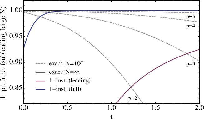
Figure 5: The subleading in $1/N$ contribution to the one-point function $\Omega(N,t)$ as a function of $t$. Everything is normalized by the extrapolation of (D.1) to $N=\infty$ (exact: $N=\infty$), and thus the black solid line representing it is flat. The gray dashed lines (exact: $N=10^{p}$) show (D.1) for $N=10^{p}$ ($p=2,3,4,5$). (5.27) is depicted by the blue line (1-inst. (full)), and the leading order term of (5.27) at large $t$ by the red line (1-inst. (leading)).

In Fig. 5, we present a plot of the subleading large-$N$ contribution to the one-point function $\Omega(N,t)$ in the double scaling limit. The result is normalized by the full nonperturbative result obtained from numerical extrapolation of the difference

$$N^{2/3}\left(\Omega(N,t)-\Omega_{0}(t)\right),$$ (D.1)

evaluated at various finite $N$ (up to $N=1,000,000$). For comparison, we also present the result for the full one-instanton contribution (5.27) and its leading order contribution at large $t$. In the plot, it appears that even the subleading large-$N$ contribution to the full one-instanton result (5.27) exhibits good agreement with the numerical results for the full contribution for $t\gtrsim 0.5$.

References

- [1] P. Di Francesco, P. H. Ginsparg and J. Zinn-Justin, “2-D Gravity and random matrices,” Phys. Rept. 254 (1995) 1 [hep-th/9306153].
- [2] I. R. Klebanov, “String theory in two-dimensions,” In *Trieste 1991, Proceedings, String theory and quantum gravity ’91* 30-101 [hep-th/9108019].
- [3] P. H. Ginsparg and G. W. Moore, “Lectures on 2-D gravity and 2-D string theory,” In *Boulder 1992, Proceedings, Recent directions in particle theory* 277-469 [hep-th/9304011].
- [4] J. McGreevy and H. L. Verlinde, “Strings from tachyons: The matrix reloaded,” JHEP 0312 (2003) 054 [hep-th/0304224].
- [5] I. R. Klebanov, J. M. Maldacena and N. Seiberg, “D-brane decay in two-dimensional string theory,” JHEP 0307 (2003) 045 [hep-th/0305159].
- [6] J. McGreevy, J. Teschner and H. L. Verlinde, “Classical and quantum D-branes in 2-D string theory,” JHEP 0401 (2004) 039 [hep-th/0305194].
- [7] S. Y. Alexandrov, V. A. Kazakov and D. Kutasov, “Nonperturbative effects in matrix models and D-branes,” JHEP 0309 (2003) 057 [hep-th/0306177].
- [8] T. Takayanagi and N. Toumbas, “A Matrix model dual of type 0B string theory in two-dimensions,” JHEP 0307 (2003) 064 [hep-th/0307083].
- [9] M. R. Douglas, I. R. Klebanov, D. Kutasov, J. M. Maldacena, E. J. Martinec and N. Seiberg, “A New hat for the matrix model,” In *Shifman, M. (ed.) et al.: From fields to strings, vol. 3* 1758-1827 [hep-th/0307195].
- [10] J. McGreevy, S. Murthy and H. L. Verlinde, “Two-dimensional superstrings and the supersymmetric matrix model,” JHEP 0404 (2004) 015 [hep-th/0308105].
- [11] T. Kuroki and F. Sugino, “New critical behavior in a supersymmetric double-well matrix model,” Nucl. Phys. B 867 (2013) 448 [arXiv:1208.3263 [hep-th]].
- [12] T. Kuroki and F. Sugino, “Supersymmetric double-well matrix model as two-dimensional type IIA superstring on RR background,” arXiv:1306.3561 [hep-th].
- [13] E. Brezin and V. A. Kazakov, “Exactly Solvable Field Theories Of Closed Strings,” Phys. Lett. B 236 (1990) 144.
- [14] M. R. Douglas and S. H. Shenker, “Strings In Less Than One-Dimension,” Nucl. Phys. B 335 (1990) 635.
- [15] D. J. Gross and A. A. Migdal, “Nonperturbative Two-Dimensional Quantum Gravity,” Phys. Rev. Lett. 64 (1990) 127; “A Nonperturbative Treatment Of Two-dimensional Quantum Gravity,” Nucl. Phys. B 340 (1990) 333.
- [16] E. Witten, “Constraints on Supersymmetry Breaking,” Nucl. Phys. B 202 (1982) 253.
- [17] I. k. Affleck, “Supersymmetry Breaking At Large ,” Phys. Lett. B 121 (1983) 245.
- [18] T. Kuroki and F. Sugino, “Spontaneous supersymmetry breaking by large- matrices,” Nucl. Phys. B 796 (2008) 471 [arXiv:0710.3971 [hep-th]].
- [19] T. Kuroki and F. Sugino, “Spontaneous supersymmetry breaking in large- matrix models with slowly varying potential,” Nucl. Phys. B 830 (2010) 434 [arXiv:0909.3952 [hep-th]].
- [20] M. Hanada, M. Hayakawa, N. Ishibashi, H. Kawai, T. Kuroki, Y. Matsuo and T. Tada, “Loops versus matrices: The Nonperturbative aspects of noncritical string,” Prog. Theor. Phys. 112 (2004) 131 [hep-th/0405076].
- [21] N. Ishibashi and A. Yamaguchi, “On the chemical potential of D-instantons in noncritical string theory,” JHEP 0506 (2005) 082 [hep-th/0503199].
- [22] T. Kuroki and F. Sugino, “Spontaneous supersymmetry breaking in matrix models from the viewpoints of localization and Nicolai mapping,” Nucl. Phys. B 844 (2011) 409 [arXiv:1009.6097 [hep-th]].
- [23] I. K. Kostov, “Strings embedded in Dynkin diagrams,” In *Cargese 1990, Proceedings, Random surfaces and quantum gravity* 135-149.
- [24] I. K. Kostov and M. Staudacher, “Multicritical phases of the model on a random lattice,” Nucl. Phys. B 384 (1992) 459 [arXiv:hep-th/9203030].
- [25] D. Gaiotto, L. Rastelli and T. Takayanagi, “Minimal superstrings and loop gas models,” JHEP 0505 (2005) 029 [hep-th/0410121].
- [26] J. Polchinski, “Combinatorics of boundaries in string theory,” Phys. Rev. D 50 (1994) 6041 [hep-th/9407031].
- [27] V. Fateev, A. B. Zamolodchikov and A. B. Zamolodchikov, “Boundary Liouville field theory. 1. Boundary state and boundary two point function,” hep-th/0001012.
- [28] J. Teschner, “Remarks on Liouville theory with boundary,” hep-th/0009138.
- [29] A. B. Zamolodchikov and A. B. Zamolodchikov, “Liouville field theory on a pseudosphere,” hep-th/0101152.
- [30] H. Kawai, T. Kuroki and Y. Matsuo, “Universality of nonperturbative effect in type 0 string theory,” Nucl. Phys. B 711 (2005) 253 [hep-th/0412004].
- [31] N. Ishibashi, T. Kuroki and A. Yamaguchi, “Universality of nonperturbative effects in noncritical string theory,” JHEP 0509 (2005) 043 [hep-th/0507263].
- [32] C. Itzykson and J. B. Zuber, “The Planar Approximation. 2.,” J. Math. Phys. 21 (1980) 411.
- [33] S. H. Shenker, “The Strength of nonperturbative effects in string theory,” In *Brezin, E. (ed.), Wadia, S.R. (ed.): The large expansion in quantum field theory and statistical physics* 809-819, and In *Cargese 1990, Proceedings, Random surfaces and quantum gravity* 191-200.
- [34] M. Marino, “Nonperturbative effects and nonperturbative definitions in matrix models and topological strings,” JHEP 0812 (2008) 114 [arXiv:0805.3033 [hep-th]].
- [35] F. David, “Phases of the large matrix model and nonperturbative effects in 2-d gravity,” Nucl. Phys. B 348 (1991) 507.
- [36] C. -T. Chan, H. Irie and C. -H. Yeh, “Stokes Phenomena and Non-perturbative Completion in the Multi-cut Two-matrix Models,” Nucl. Phys. B 854 (2012) 67 [arXiv:1011.5745 [hep-th]].
- [37] R. Dijkgraaf, E. P. Verlinde and H. L. Verlinde, “Matrix string theory,” Nucl. Phys. B 500 (1997) 43 [arXiv:hep-th/9703030].
- [38] N. Seiberg and D. Shih, “Flux vacua and branes of the minimal superstring,” JHEP 0501 (2005) 055 [hep-th/0412315].
- [39] N. Seiberg, “Observations on the moduli space of two dimensional string theory,” JHEP 0503 (2005) 010 [hep-th/0502156].
- [40] A. Mukherjee and S. Mukhi, “ matrix models: Equivalences and open-closed string duality,” JHEP 0510 (2005) 099 [hep-th/0505180].
- [41] T. Kuroki and F. Sugino, “T duality of the Zamolodchikov-Zamolodchikov brane,” Phys. Rev. D 75 (2007) 044008 [hep-th/0612042].
- [42] E. Witten, “Two-dimensional gauge theories revisited,” J. Geom. Phys. 9 (1992) 303 [hep-th/9204083].
- [43] G. Szego, “Orthogonal Polynomials,” 4th ed., Providence: American Mathematical Society (1975) 432p.
- [44] M. Marino, R. Schiappa and M. Weiss, “Nonperturbative Effects and the Large-Order Behavior of Matrix Models and Topological Strings,” Commun. Num. Theor. Phys. 2 (2008) 349 [arXiv:0711.1954 [hep-th]].
- [45] M. Marino, R. Schiappa and M. Weiss, “Multi-Instantons and Multi-Cuts,” J. Math. Phys. 50 (2009) 052301 [arXiv:0809.2619 [hep-th]].
- [46] R. Schiappa and R. Vaz, “The Resurgence of Instantons: Multi-Cuts Stokes Phases and the Painleve II Equation,” arXiv:1302.5138 [hep-th].
- [47] S. Pasquetti and R. Schiappa, “Borel and Stokes Nonperturbative Phenomena in Topological String Theory and Matrix Models,” Annales Henri Poincare 11 (2010) 351 [arXiv:0907.4082 [hep-th]].
- [48] I. Aniceto, R. Schiappa and M. Vonk, “The Resurgence of Instantons in String Theory,” Commun. Num. Theor. Phys. 6 (2012) 2, 339 [arXiv:1106.5922 [hep-th]].
- [49] G. V. Dunne and M. Unsal, “Resurgence and Trans-series in Quantum Field Theory: The CP(N-1) Model,” JHEP 1211 (2012) 170 [arXiv:1210.2423 [hep-th]].
- [50] G. V. Dunne and M. Unsal, “Generating Energy Eigenvalue Trans-series from Perturbation Theory,” arXiv:1306.4405 [hep-th].
- [51] A. Cherman, D. Dorigoni, G. V. Dunne and M. Unsal, “Resurgence in QFT: Unitons, Fractons and Renormalons in the Principal Chiral Model,” arXiv:1308.0127 [hep-th].
- [52] G. Basar, G. V. Dunne and M. Unsal, “Resurgence theory, ghost-instantons, and analytic continuation of path integrals,” arXiv:1308.1108 [hep-th].
- [53]