Orbits in a stochastic Goodwin-Lotka-Volterra model

Abstract

This paper examines the cycling behavior of a deterministic and a stochastic version of the economic interpretation of the Lotka-Volterra model, the Goodwin model. We provide a characterization of orbits in the deterministic highly non-linear model. We then study the cycling behavior for a stochastic version, where a Brownian noise is introduced via an heterogeneous productivity factor. Sufficient conditions for existence of the system are provided. We prove that the system produces cycles around an equilibrium point in finite time for general volatility levels, using stochastic Lyapunov techniques for recurent domains. Numerical insights are provided.

Keywords: Lotka-Volterra model; Goodwin model; Brownian motion; Random perturbation; Business cycles; Stochastic Lyapunov techniques.

1 Introduction

The Lotka-Volterra equation is at the heart of population dynamics, but also possesses a famous economic interpretation. Introduced by Richard Goodwin [10] in 1967, the model in its modern form [6] reduces to the planar oscillator on a subset $D$ of $\mathbb{R}_{+}$:

$$\left\{\begin{array}[]{ll}dx_{t}&=x_{t}\left(\Phi(y_{t})-\alpha\right)dt\\ dy_{t}&=y_{t}\left(\kappa(x_{t})-\gamma\right)dt\end{array}\right.\;,$$ (1)

where $x_{t}$ denotes the wage share of the working population and $y_{t}$ the employment rate, $\alpha$ and $\gamma$ are constant, and the following assumption is made on $\kappa$ and $\Phi$.

Assumption 1.

Consider system (1).

1. $\Phi\in{\cal C}^{2}([0,1))$, $\Phi^{\prime}(y)>0$, $\Phi^{{}^{\prime\prime}}(y)\geq 0$ for all $y\in[0,1)$, $\Phi(0)<\alpha$ and $\lim_{y\to 1^{-}}\Phi(y)=+\infty$.

2. $\kappa\in{\cal C}^{2}(\mathbb{R}_{+})$, $-\infty<\kappa^{\prime}(x)<0$ for all $x\in\mathbb{R}_{+}$, $\kappa(0)>\gamma$ and $\lim_{x\to+\infty}\kappa(x)=-\infty$.

Lemma 1 below asserts that Assumption 1 is sufficient to have $(x_{t},y_{t})\in D:=\mathbb{R}^{*}_{+}\times(0,1)$ for any $t\geq 0$ if $(x_{0},y_{0})\in D$. This property preserves the above interpretation for $x$ and $y$: the employment rate cannot exceed one for obvious reasons, but the wage share can, depending on the chosen economic assumptions, see [11]. This distinctive feature of the economic version (1) on its biological counterpart follows from a construction based on assumptions describing a closed capitalist economy. It can be done in three steps:

1. Assume a Leontief production function $P_{t}=\min(K_{t}/\nu;a_{t}y_{t}N_{t})$ with full utilization of capital, i.e., $K_{t}/\nu=a_{t}y_{t}N_{t}$. Here, $P_{t}$ is the yearly output, $K_{t}$ the invested capital, $\nu>0$ a capital-to-output ratio, $a_{t}:=a_{0}\exp(\alpha t)$ is the average productivity of workers and $N_{t}:=N_{0}\exp(\beta t)$ is the size of the labor class.

2. The capital depreciates and receives investment, i.e., $dK_{t}/dt=(\kappa(x_{t})-\delta)K_{t}$, where $\delta>0$ is the depreciation rate and $\kappa$ the investment function. Goodwin [10] originally invokes Say’s law, i.e., $\kappa~{}:~{}x\in\mathbb{R}_{+}\mapsto(1-x)/\nu$.

3. Assume a reserve army effect for wage negotiation of the form $dw_{t}=\Phi(y_{t})w_{t}dt$ where $w_{t}:=a_{t}x_{t}$ represents the real wage of the total working population, and $\Phi$ is the Phillips curve.

Defining $\gamma:=\alpha+\beta+\delta$ allows to retrieve (1) for $(x_{t},y_{t}):=(w_{t}/a_{t},K_{t}/(\nu a_{t}N_{t}))$. The class-struggle model (1) has been extensively studied because it allows to generate endogenous real business cycles affecting the production level $P_{t}$, e.g. [8, 9, 11, 15, 28, 29]. On this matter, Goodwin himself conceded that the model is “starkly schematized and hence quite unrealistic” [10]. It hardly connects with irregular observed trajectories, see [13, 22].

The objective of this paper is thus to study the following perturbed version of (1) by a standard Brownian motion $(W_{t})_{t\geq 0}$ on a stochastic basis $(\Omega,{\cal F},\mathbb{P})$:

$$\left\{\begin{array}[]{ll}dx_{t}&=x_{t}\left((\Phi(y_{t})-\alpha+\sigma^{2}(y_{t}))dt+\sigma(y_{t})dW_{t}\right)\\ dy_{t}&=y_{t}\left((\kappa(x_{t})-\gamma+\sigma^{2}(y_{t}))dt+\sigma(y_{t})dW_{t}\right)\end{array}\right.\;,$$ (2)

where $\sigma$ is a positive function of $y$ bounded by $\sigma_{0}>0$, and the filtration ${\cal F}_{t}$ is generated by paths of $W$. The form of $\sigma$ is discussed in Remark 2 after. A stronger condition, Assumption 3, is assumed later on the behavior of $\sigma$ to ensure that solutions of (2) remain in $D$. The example of Section 5 will also illustrate how such condition can hold. We modify the economic development (I), (II) and (III) by introducing the perturbation on one assumption, namely we assume that for $t\geq 0$,

$$da_{t}:=a_{t}d\alpha_{t}=a_{t}\left(\alpha dt-\sigma(y_{t})dW_{t}\right)\;,\quad a_{0}\geq 0\;,$$ (3)

instead of $da_{t}=a_{t}\alpha dt$. Using Itô formula with (3) in the previous reasoning retrieves (2). Productivity is one of the few exogenous parameters of the model, and one of those that were significantly invoked as influencial over business cycles, e.g. [7, 12]. Without arguing for the pertinence of that particular assumption, we simply suggest here that a standard continuous perturbation in this crucial parameter seems a good starting point.

To our knowledge, this is the first attempt to consider random noise in Goodwin interpretation of the famous prey-predator model. To stay in the spirit of the economic application, the present paper studies the cyclical behavior of the deterministic system (1) and the stochastic version (2). Namely, our contribution are as follows, developed in the present order:

• In Section 2, we fully characterize solutions of (1) and the period of their orbits. This generalizes standard results on Lotka-Volterra systems to bounded domains of existence.

• In Section 3, we provide existence conditions for regular solutions of (2). We use the entropy of (1) to estimate the deviation induced by (3). We provide a definition of stochastic orbits for (2). The proof that solutions of (2) draw stochastic orbits in finite time around a unique point is given in Section 4.

Our contribution has to be put in contrast with numerous studies of random perturbations of the Lotka-Volterra system. Apart from the obviously different origin of perturbations in the model, attention was mainly given to systems like (2) for its asymptotic behavior (e.g., [18, 21, 24]), regularity, persistence and extinction of species (e.g., [4, 20, 24, 25]), and the addition of regimes, jumps or delay (e.g., [2, 19, 31]). Here, we attempt to provide a relevant description of trajectories $(x_{t},y_{t})$ and indirectly $P_{t}$, namely a cyclical behavior. This is done using stochastic Lyapunov techniques for recurrent domains as described in [17, 27]. By conveniently dividing the domain $D$, we obtain that almost every trajectory “cycles” around a point in finite time. The $L_{1}$-boundedness is out of reach with our method, but numerical simulations are presented in Section 5, not only to provide expectation of cycles, but also allow to conjecture a limit cycle phenomenon for the expectation of $(x_{t},y_{t})$. It is somewhat unclear how Assumption 1 and late Assumption 3 on $\Phi$, $\kappa$ and $\sigma$, are relevant in these results. We show below thatthey are sufficient to obtain existence of regular solutions to (2). This actually emphasizes the role played by the entropy of the deterministic system in the well-posedness of the stochastic system and as a natural measure for perturbation.

2 Deterministic orbits

According to Assumption 1, there exists only one non-hyperbolic equilibrium point to (1) in $D$ given by $(\hat{x},\hat{y}):=(\kappa^{-1}(\gamma),\Phi^{-1}(\alpha))$. On the boundary of $D$, there exists also an additional equilibrium $(0,0)$ which is eluded along the paper.

Definition 1.

Let $V_{1},V_{2}$ and $V$ be three functions defined by $V~{}:~{}(x,y)\in\mathbb{R}^{*}_{+}\times(0,1)\mapsto V_{1}(x)+V_{2}(y)$ and

$$V_{1}~{}:~{}x\in\mathbb{R}^{*}_{+}\mapsto\int_{\hat{x}}^{x}\frac{\kappa(\hat{x})-\kappa(s)}{s}ds\;,\quad V_{2}~{}:~{}y\in(0,1)\mapsto\int_{\hat{y}}^{y}\frac{\Phi(s)-\Phi(\hat{y})}{s}ds\;.$$

Lemma 1.

Let $(x_{0},y_{0})\in D$. Let Assumption 1 hold. Then a solution $(x_{t},y_{t})$ to (1) starting at $(x_{0},y_{0})$ at $t=0$ describes closed orbits given by the set of points $\{(x,y)\in D~{}:~{}V(x,y)=V(x_{0},y_{0})\}$, and $(x_{t},y_{t})\in D$ for all $t\geq 0$.

Proof.

It is well-known [11] that $V$ is a Lyapunov function and a constant of motion for system (1): $V_{1}$ and $V_{2}$ take non-negative values with $V_{1}(\hat{x})=V_{2}(\hat{y})=0$, and $dV/dt(x,y)=0$. Additionally, under Assumption 1.(i)-(ii),

$$\lim_{x\uparrow+\infty}V_{1}(x)=\lim_{x\downarrow 0^{+}}V_{1}(x)=\lim_{y\uparrow 1^{-}}V_{2}(y)=\lim_{y\downarrow 0^{+}}V_{2}(y)=+\infty\;,$$ (4)

so that for any $(x_{0},y_{0})\in D$, $V(x_{0},y_{0})<+\infty$ and the solution stays in $D$.

∎

The value of $V$ characterizing an orbit, it is in bijection with its period. The following generalizes [14].

Theorem 1.

Let $(x_{t},y_{t})_{t\geq 0}$ be a solution to (1) satisfying Assumption 1, with $(x_{0},x_{0})\in D\backslash\{(\hat{x},\hat{y})\}$. Let $V_{0}:=V(x_{0},y_{0})$, and $\underline{x}<\bar{x}$ the two solutions to equation $V_{1}(x)=V_{0}$. Define three functions $F_{1},F_{2},G$ by

$$F_{1}~{}:~{}u\in\mathbb{R}\mapsto V_{2}(\Phi^{-1}(u^{+}+\alpha))\;,\quad F_{2}~{}:~{}u\in\mathbb{R}\mapsto V_{2}(\Phi^{-1}(-u^{-}+\alpha))\;,\quad G~{}:~{}z\in\mathbb{R}\mapsto V_{0}-V_{1}(e^{z})\;.$$

Then $(x_{T},y_{T})=(x_{0},y_{0})$ for $T$ defined by

$$T(V_{0}):=\int_{log(\underline{x})}^{\log(\bar{x})}\frac{1}{F_{1}^{-1}(G(z))}-\frac{1}{F_{2}^{-1}(G(z))}dz\;.$$ (5)

Proof.

Let $(x_{0},y_{0})\in D\backslash\{(\hat{x},\hat{y})\}$, $V_{0}=V(x_{0},y_{0})>0$ and $(x_{t},y_{t})$ a solution to (1) starting at $(x_{0},y_{0})$. According to Lemma 1, $V_{1}(x_{t})=V_{0}$ implies $V_{2}(y_{t})=0$. Then $\{x\in\mathbb{R}_{+}~{}:~{}x_{t}=x\text{ for some }t\geq 0\}=[\underline{x},\bar{x}]=:I$. Homogeneity of (1) allows to set $(x_{0},y_{0})=(\underline{x},\hat{y})$ without loss of generality. Let $T_{1}:=\inf\{t\geq 0~{}:~{}x_{t}=\bar{x}\}$. For $t\in[0,T_{1}]$, $(x_{t},y_{t})\in[\underline{x},\bar{x}]\times[\hat{y},\bar{y}]$, with $\bar{y}$ such that $V_{2}(\bar{y})=V_{0}$. Let $z_{t}:=\log(x_{t})$ for $t\geq 0$. Then (1) rewrites $dz=(\Phi(y)-\alpha)dt$, $y=\Phi^{-1}(dz/dt+\alpha)$ and we get

$$\frac{d^{2}z}{dt^{2}}=\Phi^{\prime}(y)\frac{dy}{dt}=\Phi^{\prime}\left(\Phi^{-1}\left(\frac{dz}{dt}+\alpha\right)\right)\Phi^{-1}\left(\frac{dz}{dt}+\alpha\right)[\kappa(e^{z})-\gamma]\;.$$

Let $u:=\Phi(y)-\alpha$ and define $\Psi:=\Phi^{\prime}\circ\Phi^{-1}\times\Phi^{-1}$, to rewrite again

$$\left\{\begin{array}[]{ll}dz/dt&=u\\ du/dt&=\Psi\left(u+\alpha\right)[\kappa(e^{z})-\gamma]\end{array}\right.\;.$$ (6)

Since $z_{t}\in[\underline{z},\bar{z}]:=[\log(\underline{x}),\log(\bar{x})]$ and $u_{t}\in[0,\Phi(\bar{y})-\alpha]$ for $t\in[0,T_{1}]$, separation of variables in (6) provides two quantities $F$ and $G$:

$$F(u):=\int_{0}^{u}\frac{s}{\Psi\left(s+\alpha\right)}ds=\int_{\underline{z}}^{z}[\kappa(e^{s})-\gamma]ds=:G(z)\;.$$ (7)

The function $F$ verifies $F(0)=G(\bar{z})=0$, is increasing on $[0,\Phi(\bar{y})-\alpha]$ and decreasing on $[\Phi(\underline{y})-\alpha,0]$ with $\underline{y}<\hat{y}$ so that $V_{2}(\underline{y})=0$. Coming back to $y=\Phi^{-1}(u+\alpha)$ we get

$$F(u)=\int_{0}^{u}\frac{s}{\Phi^{\prime}(\Phi^{-1}(s+\alpha))\Phi^{-1}(s+\alpha)}ds=\int_{\hat{y}}^{\Phi^{-1}(u+\alpha)}\frac{\Phi(s)-\Phi(\hat{y})}{s}ds=V_{2}(\Phi^{-1}(u+\alpha))\;,$$

implying that $F(u)\in[0,V(\underline{x},\hat{y})]$ for $u\in[\Phi(\underline{y})+\alpha,\Phi(\bar{y})+\alpha]$. We can write $F=F_{1}+F_{2}$ where $F_{1}$ and $F_{2}$ are the two restrictions of $F$ on $\mathbb{R}_{+}$ and $\mathbb{R}_{-}$ respectively. Notice that if $t\in[0,T_{1}]$, then $u_{t}:=\Phi(y_{t})+\alpha\in[0,\Phi(\bar{y}+\alpha)]$. Thus, $F_{1}(u_{t})$ is a strictly increasing function of $t$ taking its values in $[0,V(\underline{x},\hat{y})]$. Getting back to $x=e^{z}$ for $G$, we have for $z\geq\underline{z}$

$$G(z):=\int_{\underline{x}}^{\hat{x}\wedge e^{z}}\frac{\kappa(s)-\gamma}{s}ds+\int_{\hat{x}\wedge e^{z}}^{e^{z}}\frac{\kappa(s)-\gamma}{s}ds=V_{0}-V_{1}(e^{z})$$

Since $\text{sign}(\kappa(x)-\gamma)=\text{sign}(\hat{x}-x)$ we have $\max_{z\in[\underline{z},\bar{z}]}G(z)=G(\log(\hat{x}))=V_{1}(\underline{x})=V(\underline{x},\hat{y})$, while minimums are given by $G(\bar{z})=G(\underline{z})=0$. This sums up with $G([\underline{z},\bar{z}])\subset[0,V_{0}]$, so we can write on this interval $F_{1}^{-1}(G(z))=u=dz/dt$ which finally gives

$$T_{1}=\int_{\underline{z}}^{\bar{z}}\frac{dz}{F_{1}^{-1}(G(z))}\;.$$

We apply the same method for the other half orbit, taking $(x_{0},y_{0})=(\bar{x},\hat{y})$ and $T_{2}:=\inf\{t\geq 0~{}:~{}x_{t}=\underline{x}\}$, to reach the other half of expression (5), i.e., $T(V_{0})=T_{1}+T_{2}$. ∎

Remark 1.

A first order approximation of (1) at $(\hat{x},\hat{y})$ provides a linear homogeneous system, which solution is trivially given by a linear combination of sines and cosines of $(-\hat{x}\Phi^{\prime}(\hat{y})\hat{y}\kappa^{\prime}(\hat{x})t)$. It follows that

$$\lim\limits_{V_{0}\rightarrow 0}T(V_{0})=\frac{2\pi}{\sqrt{-\hat{x}\Phi^{\prime}(\hat{y})\hat{y}\kappa^{\prime}(\hat{x})}}>0\;.$$

3 Stochastic Goodwin model

We study a specific case of (2) where the deterministic part cancels at a unique point in $D$ defined by $(\tilde{x},\tilde{y}):=(\kappa^{-1}(\gamma-\sigma^{2}(\tilde{y})),\tilde{y})$ where $\tilde{y}$ comes from the following.

Assumption 2.

There is a unique $\tilde{y}\in(0,1)$ such that $\Phi(\tilde{y})-\alpha+\sigma^{2}(\tilde{y})=0$

For a stochastic differential equation to have a unique global solution for any given initial value, functions $\Phi$ and $\kappa$ are generally required to satisfy linear growth and local Lipschitz conditions, see [17]. We can however consider the following Theorem of Khasminskii [17], which is a reformulation of Theorem 3.4, Theorem 3.5 and Corollary 3.1 of [17] to our context.

Theorem 2.

Consider the following stochastic differential equation for $z$ taking values in $\mathbb{R}^{2}_{+}$:

$$dz_{t}=\mu(z_{t})dt+\sigma(z_{t})dW_{t}\;.$$ (8)

Let $(D_{n})_{n\geq 1}$ be an increasing sequence of open sets, and $(K_{n})_{n\geq 1}$ a sequence of constants, verifying

1. $\bar{D}_{n}\subset D$ for all $n\geq 1$,

2. $\bigcup_{n}D_{n}=D$.

3. For any $n\geq 1$, functions $\mu$ and $\sigma$ are Lipschitz on $D_{n}$ and verify $|\mu(z)|+|\sigma(z)|\leq K_{n}(1+|z|)$ for any $z\in D_{n}$.

Let $\varphi\in{\cal C}^{1,2,2}(\mathbb{R}_{+}\times D)$ and $(K,k)\in\mathbb{R}_{+}^{2}$ be such that, denoting ${\cal L}^{z}$ the generator associated with (8),

1. ${\cal L}^{z}\varphi(t,z_{t})\leq K\varphi(t,z_{t})+k$ on the set $\mathbb{R}_{+}\times D$,

2. $\lim_{n}\inf_{D\backslash D_{n}}\varphi(t,z)=+\infty$ for any $t\geq 0$.

Then for any $z\in D$, there exists a regular adapted solution to (8), unique up to null sets, with the Markov property and verifying $z_{t}\in D$ for all $t\geq 0$ almost surely.

To satisfy conditions (a) to (e), we study (2) under the additional sufficient growth conditions.

Assumption 3.

There exist two positive constants $K,k$ such that

1. $\sigma^{2}(y)\Phi^{\prime}(y)\leq KV_{2}(y)+k$ for all $y\in(0,1)$,

2. $-x\kappa^{\prime}(x)-\kappa(x)\leq KV_{1}(x)+k$ for all $x\in\mathbb{R}_{+}^{*}$.

Remark 2.

Assumption 3.(i) involves both $\Phi$ and $\sigma$ to ensure that $y_{t}\in(0,1)$ for all $t\geq 0$ almost surely. Assumption 3.(ii) holds for polynomial growth of $\kappa$, suiting the classical conditions of existence on $\mathbb{R}_{+}$ for $x_{t}$. The dependence of $\sigma$ could be generalized to $x$ in full generality, implying a stronger condition than (ii). We refrain from doing this easy extension, emphasizing the unavoidable dependence in $y$.

For $\varphi\in{\cal C}^{1,2,2}(\mathbb{R}_{+}\times D)$, we recall the diffusion operator associated with (2) by

$$\begin{array}[]{lll}{\cal L}\varphi(t,x,y)&:=&\left[\frac{\partial\varphi}{\partial t}+\frac{\partial\varphi}{\partial x}x(\Phi(y)-\alpha+\sigma^{2}(y))+\frac{\partial\varphi}{\partial y}y(\kappa(x)-\gamma+\sigma^{2}(y))\right.\\ &&\left.+\frac{\sigma^{2}(y)}{2}\left(\frac{\partial^{2}\varphi}{\partial x^{2}}x^{2}+\frac{\partial^{2}\varphi}{\partial y^{2}}y^{2}+2\frac{\partial^{2}\varphi}{\partial x\partial y}xy\right)\right](t,x,y).\end{array}$$ (9)

Theorem 3.

Let $(x_{0},y_{0})\in D$. Let Assumptions 1, 6 and 3 hold. Then there exists a solution $(x_{t},y_{t})_{t\geq 0}$ to (2) staying in $D$ almost surely.

Proof.

Let us show that conditions (a) to (e) of Theorem 2 are fulfilled. Consider the sequence of sets $(D_{n})_{n\geq 1}$ defined by $D_{n}=(1/(n+1),n)\times(1/(n+1),1-1/(n+1))$. For any $n\geq 1$, $D_{n}$ is open and $D_{n}\subset D_{n+1}$. (a) and (b) are satisfied with the limit $D=\mathbb{R}_{+}^{*}\times(0,1)$. According to Assumption 1, one can always find $K_{n}$ big enough such that $\max\{|\Phi(y)-\alpha|;|\kappa(x)-\gamma|\}\leq K_{n}$ for any $(x,y)\in D_{n}$, and ensures the local Lipschitz condition (c).

Now consider $V$ of Definition 1 which is ${\cal C}^{1,2,2}$ on $D$. Applying (9),

$${\cal L}V(x,y)= \left[\kappa(\hat{x})-\kappa(x)\right](\Phi(y)-\alpha+\sigma^{2}(y))+\left[\Phi(y)-\Phi(\hat{y})\right](\kappa(x)-\gamma+\sigma^{2}(y))$$

$$+\left(\left[\kappa(x)-\kappa(\hat{x})-x\kappa^{\prime}(x)\right]+\left[\Phi(\hat{y})-\Phi(y)+y\Phi^{\prime}(y)\right]\right)\sigma^{2}(y)/2\;.$$

Since $\alpha=\Phi(\hat{y})$ and $\gamma=\kappa(\hat{x})$,

$${\cal L}V(x,y)=\left(\left[\kappa(\hat{x})-\kappa(x)-x\kappa^{\prime}(x)\right]+\left[\Phi(y)-\Phi(\hat{y})+y\Phi^{\prime}(y)\right]\right)\sigma^{2}(y)/2\;.$$ (10)

Assumption 3 implies ${\cal L}V(x,y)\leq\max(\sigma_{0}^{2}/2;2K)V(x,y)+2k$ for two positive constants $K,k$, checking condition (d). From Definition 1,

$$\inf_{x\in[0,+\infty)}V(x,y)=V_{2}(y)+\inf_{x\in[0,+\infty)}V_{1}(x)=V_{2}(y)$$

which implies that $\inf_{D\backslash D_{n}}V(x,y)\geq\inf\{V_{2}(y)~{}:~{}\max\{y,1-y\}\leq 1/n\}$, the latter going to infinity with $n$, recall (4). Similarly, $\inf_{y\in(0,1)}V(x,y)$ goes to infinity as $x$ goes to $0$ or $+\infty$. Condition (e) is then satisfied, which allows to apply Theorem 2.

∎

Remark 3.

Notice that $\tilde{y}<\hat{y}$ and thus $\tilde{x}>\hat{x}$. Following Assumption 1, (10) at $(\tilde{x},\tilde{y})$ provides ${\cal L}V(\tilde{x},\tilde{y})>0$. It is straightforward that (2) has no equilibrium point in $D$, nor on its boundary $\{0\}\times(0,1)\cup\mathbb{R}_{+}^{*}\times\{0,1\}$. If the point $(0,0)$ cancels (2), we highlight that ${\cal L}V(0,0)<0$ and by continuity, it holds on a small region $[0,\varepsilon)^{2}$. Recalling (4) implies that $(x_{t},y_{t})$ will diverge from $(0,0)$ almost surely if $(x_{0},y_{0})\in D$.

A solution to (2) can be pictured as a trajectory continuously jumping from an orbit of (1) to another. Along this idea, $V$ provides an estimate on trajectories, and can be related via Theorem 1 to the period $T$.

Theorem 4.

Let $(x_{0},y_{0})\in D$, $V_{0}:=V(x_{0},y_{0})$, and $\left(x_{t},y_{t}\right)_{t\geq 0}$ be a regular solution to (2). We first introduce a constant $0\leq\rho\leq V_{0}$, the set $D(V_{0},\rho):=\{(x,y)\in D~{}:~{}|V(x,y)-V_{0}|\leq\rho\}\subset D$ and the stopping time $\tau_{\rho}:=\inf\{t>0~{}:~{}(x_{t},y_{t})\notin D(V_{0},\rho)\}$. We then introduce two finite constants

$$R(V_{0},\rho):=\max\limits_{D(V_{0},\rho)}\left\{\sigma^{2}(y)\left(\kappa(\hat{x})-\kappa(x)-x\kappa^{\prime}(x)+y\Phi^{\prime}(y)+\Phi(y)-\Phi(\hat{y})\right)\right\}$$

and

$$I(V_{0},\rho):=\max\limits_{D(V_{0},\rho)}\left\{\sigma^{2}(y)\left(\kappa(\hat{x})-\kappa(x)+\Phi(y)-\Phi(\hat{y})\right)^{2}\right\}\;.$$

Then for all $\mu>0$

$$\mathbb{P}\left[{\tau_{\rho}>\Theta(\rho,\mu)}\right]\geq\left(1-\frac{I(V_{0},\rho)}{\mu^{2}}\right)\quad\text{ for }\quad\Theta(\rho,\mu):=\frac{2\left(\mu^{2}+\mu\sqrt{\mu^{2}+2\rho R(V_{0},\rho)}+\rho R(V_{0},\rho)\right)}{(R(V_{0},\rho)\sigma)^{2}}\;.$$ (11)

Proof.

Fix $\mu>0$. Now we define the ${\cal F}_{\tau_{\rho}}$-measurable set $A_{\mu}=\left\{\omega\in\Omega:\sup_{0<t\leq\tau_{\rho}}\big{|}M_{t}(\omega)\big{|}\leq\mu\right\}$ where $(M_{t})_{t\geq 0}$ is a martingale defined by $M_{t}=0$ for $t=0$ and for $t>0$ by

$$M_{t}=\frac{1}{\sqrt{t}}\int_{0}^{t}\sigma(y_{s})\left(\kappa(\hat{x})-\kappa(x_{s})+\Phi(y_{s})-\Phi(\hat{y})\right)dW(s)\;.$$

The process $M$ is not right-continuous at $t=0$ but still verifies $\mathbb{E}\left[M_{t}^{2}\right]\leq I(V_{0},\rho)$ for all $0<t\leq\tau_{\rho}$. The property holds by replacing $M_{t}$ by its càdlàg representation. Doob’s martingale inequality can then be applied: $\mathbb{P}\left[{A_{\mu}}\right]\geq 1-I(V_{0},\rho)/\mu^{2}$. At last, using Itô’s formula, we have from (10):

$$|V(x_{t},y_{t})-V_{0}| \leq \frac{1}{2}\int_{0}^{t}\sigma^{2}(y_{s})\left|\kappa(\hat{x})-\kappa(x_{s})-x_{s}\kappa^{\prime}(x_{s})+y_{s}\Phi^{\prime}(y_{s})+\Phi(y_{s})-\Phi(\hat{y})\right|ds$$

$$+\bigg{|}\int_{0}^{t}\sigma(y_{s})\left(\kappa(\hat{x})-\kappa(x_{s})+\Phi(y_{s})-\Phi(\hat{y})\right)dW_{s}\bigg{|}$$

so that on $\{(t,\omega)\in\mathbb{R}_{+}\times\Omega~{}:~{}(t,\omega)\in A_{\mu}\times[0,\tau_{\rho}(\omega)]\}$ $|V(x_{t},y_{t})-V_{0}|\leq\frac{1}{2}R(V_{0},\rho)t+\mu\sqrt{t}=:S(t)$ almost surely. Also, $|e(t,\omega)|\leq\rho$ on that set. Put in another way, $\tau_{\rho}>S^{-1}(\rho)=:\Theta(\rho)$ on $A_{\mu}$. According to Bayes rule,

$$\mathbb{P}\left[{\tau_{\rho}>\Theta(\rho)}\right]\geq\mathbb{P}\left[{\tau_{\rho}>\Theta(\rho)\big{|}A_{\mu}}\right]\mathbb{P}\left[{A_{\mu}}\right]\geq\mathbb{P}\left[{A_{\mu}}\right]\geq\left(1-\frac{I(V_{0},\rho)}{\mu^{2}}\right)$$

∎

We now introduce the main result of the paper. We provide the following tailor-made definition for the cycling behavior of (2).

Definition 2.

Let $(x^{*},y^{*})\in E\subseteq\mathbb{R}^{2}$ and $(x_{0},y_{0})\in E\backslash\{(x^{*},y^{*})\}$. Let $(x_{t},y_{t})$ be a stochastic process starting at $(x_{0},y_{0})$ staying in $E$ almost surely. We then introduce $(\rho_{t})_{t\geq 0}$ the angle between $[x_{t}-x^{*},y_{t}-y^{*}]^{\top}$ and $[x_{0}-x^{*},y_{0}-y^{*}]^{\top}$. Let $S:=\inf\{t>0~{}:~{}|\rho_{t}|\geq 2\pi\text{ or }(x_{t},y_{t})=(x^{*},y^{*})\}$ be a stopping time (a stochastic period). Then, the process $(x_{t},y_{t})$ is said to orbit stochastically around $(x^{*},y^{*})$ in $E$ if $S<+\infty$ almost surely.

Theorem 5.

Let $(x_{0},y_{0})\in D\backslash\{(\tilde{x},\tilde{y})\}$ and $(x_{t},y_{t})$ a solution to (2) starting at $(x_{0},y_{0})$. Then $(x_{t},y_{t})$ orbits stochastically around $(\tilde{x},\tilde{y})$ in $D$.

More precisely the system (2) produces clockwise orbits inside $D$. The angle $\rho_{t}$ is only defined if $(x_{t},y_{t})\neq(\tilde{x},\tilde{y})$. This can be ensured by either proving that $(x_{t},y_{t})\neq(\tilde{x},\tilde{y})$ for all $t\geq 0$ almost surely, or by defining $S$ as in Definition 2. See also Remark 4 The proof of Theorem 5 is removed to Section 4.

4 Proof of Theorem 5

4.1 Preliminary definitions and results

Recall that the probability space is given by $(\Omega,{\cal F},\mathbb{P})$ with the filtration generated only by $W$ is completed with null sets. Our proof, although unwieldy, allows us to describe precisely the possible trajectories of solutions of (2). it consists in defining subregions $(R_{i})_{i}$ of the domain $D$, see Definition 4 below illustrated by Fig. 1, and prove that the process exits from them in finite time by the appropriate frontier. According to Theorem 3 any regular solution of (2) is a Markov process. We then repeatedly change the initial condition of the system, as equivalent of a time translation and use Definition 5 herefater. We obtain recurrence properties via Theorem 3.9 in [17]. Since it is repeatedly used hereafter, we provide here a version suited to our context.

Theorem 6.

Let $(x_{t},y_{t})_{t\geq 0}$ be a regular solution of (2) in $D$, starting at $(x_{0},y_{0})\in U$, for some $U\subset D$. Let $\varphi(t,x,y)\in{\cal C}^{1,2,2}(\mathbb{R}_{+}\times U)$ verifying $\varphi(t,x,y)\geq 0$ for all $(t,x,y)\in U$ and ${\cal L}\varphi(s,x,y)\leq-\varphi(s)$ where $\varphi(s)\geq 0$ and $\lim_{t}\int_{0}^{t}\varphi(s)ds=+\infty$. Then $(x_{t},y_{t})$ leaves the region $U$ in finite time almost surely.

Definition 3.

Let $f$ be defined by $f~{}:~{}x\in\mathbb{R}_{+}\mapsto f(x):=\Phi^{-1}(\alpha-\gamma+\kappa(x))$ as a concave decreasing function. For a solution $(x_{t},y_{t})$ to (2), we define $\theta_{t}:=y_{t}/x_{t}$ the finite variation process verifying $d\theta_{t}=\theta_{t}\left(\kappa(x)-\gamma+\alpha-\Phi(y)\right)dt=\theta_{t}\left(\Phi(f(x))-\Phi(y)\right)dt$. Additionally, let $\tilde{\theta}:=\tilde{y}/\tilde{x}$.

Definition 4.

We define eight sets $(R_{i})_{i=1,\ldots,8}$ such that $\bigcap_{i=1}^{8}R_{i}=(\tilde{y},\tilde{x})$ and $\bigcup_{i=1}^{8}R_{i}=D$, by

$$\left\{\begin{array}[]{l}R_{1}:=\{(x,y)\in D~{}:~{}y\geq\tilde{y}\;\mbox{ and }\;\theta_{t}\leq\tilde{\theta}\}\\ R_{2}:=\{(x,y)\in D~{}:~{}f(x)\leq y\leq\tilde{y}\}\\ R_{3}:=\{(x,y)\in D~{}:~{}y\leq f(x)\;\mbox{ and }\;x\geq\tilde{x}\}\\ R_{4}:=\{(x,y)\in D~{}:~{}x\leq\tilde{x}\;\mbox{ and }\;\theta\leq\tilde{\theta}\}\\ R_{5}:=\{(x,y)\in D~{}:~{}y\leq\tilde{y}\;\mbox{ and }\;\theta_{t}\geq\tilde{\theta}\}\\ R_{6}:=\{(x,y)\in D~{}:~{}\tilde{y}\leq y\leq f(x)\}\\ R_{7}:=\{(x,y)\in D~{}:~{}y\geq f(x)\;\mbox{ and }\;x_{t}\leq\tilde{x}\}\\ R_{8}:=\{(x,y)\in D~{}:~{}y\geq f(x)\;\mbox{ and }\;x_{t}\leq\tilde{x}\}.\end{array}\right.$$

Definition 5.

Let $(x_{t},y_{t})$ be a solution to (2) starting at $(x_{0},y_{0})=(x,y)\in D$. For any $i\in\{1,\ldots,8\}$, we define the stopping times $\tau_{i}(x,y):=\inf\{t\geq 0~{}:~{}(x_{t},y_{t})\in R_{i}\}$.

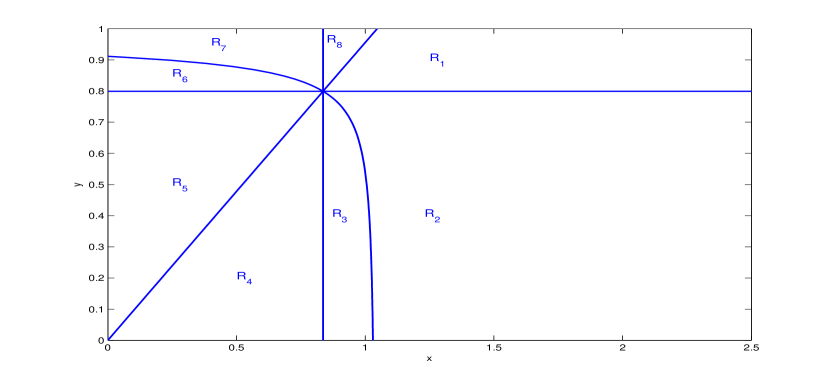
Figure 1: Covering of $D:=\mathbb{R}_{+}^{*})\times(0,1)$ by $(R_{i})_{i=1\ldots 8}$. Since $f(0)<1$ and $\lim_{y\uparrow 1}\Phi(y)=+\infty$, the graph illustrates the general case.

Remark 4.

It seems rather clear that the point $(\tilde{x},\tilde{y})$ is not reached in finite time with a positive probability. In the following, the fact that ${\cal L}V(x,y)>\varepsilon$ for some small $\varepsilon>0$ in a neighborhood of $(\tilde{x},\tilde{y})$ implies that $(\tilde{x},\tilde{y})$ is not a limit to almost every path of a solution to (2), recall Remark 3.

To ease the reading of the proof of Theorem 5 which follows from the following Propositions 1 to 10, we divide it in four quadrants around $(\tilde{x},\tilde{y})$. We first prove that the process cycles, even in infinite time, for some particular starting points.

Proposition 1.

If $(x_{0},y_{0})\in R_{1}$, then $\mathbb{P}\left[{\tau_{8}(x_{0},y_{0})\leq\tau_{7}(x_{0},y_{0})}\right]=0$. If $(x_{0},y_{0})\in R_{5}$, then $\mathbb{P}\left[{\tau_{4}(x_{0},y_{0})\leq\tau_{3}(x_{0},y_{0})}\right]=0$.

Proof.

This is a direct consequence of the absence of Brownian motion in $\theta$. Take $(x_{0},y_{0})\in R_{1}$. Then on $[0,\tau_{3}(x_{0},y_{0})]$, the process $\theta$ is non increasing almost surely, meaning that $R_{8}$ cannot be reached without first crossing region $R_{7}$. The other side is identical. ∎

Remark 5.

Proposition 1 holds even if $\tau_{i}=+\infty$, for any $i$ involved. It also implies that if $(x_{0},y_{0})\in R_{1}\cup R_{5}$, then $\tau_{i}(x_{0},y_{0})\leq\tau_{j}(x_{0},y_{0})$ almost surely for $j\in\{mod(i+1,8)\}$.

4.2 Eastern quadrant

We ought to prove that for $(x_{0},y_{0})\in R_{1}$, the process reaches $R_{3}$ in finite time almost surely.

Proposition 2.

If $(x_{0},y_{0})\in R_{1}$ then $\mathbb{P}\left[{\tau_{2}(x_{0},y_{0})<+\infty}\right]=1$.

Proof.

Let $\varphi~{}:~{}y\in[0,1]\mapsto\sqrt{y}$. Then $\varphi(y)\geq\varphi(\tilde{y})>0$ for any $y$ such that $(x,y)\in R_{1}$. Moreover,

$${\cal L}\varphi(y)=\frac{\varphi(y)}{2}\left(\kappa(x)-\gamma+\frac{3}{4}\sigma^{2}(y)\right)\leq-\frac{\sigma^{2}(\tilde{y})\varphi(y)}{8}\leq-\frac{\sigma^{2}(\tilde{y})h(\tilde{y})}{8}<0\;.$$

Theorem 6 stipulates that $(x_{t},y_{t})$ leaves $R_{1}$ in finite time almost surely which is only possible via $R_{2}$ according to Proposition 1. Reaching the boundary is prevented by Theorem 3.

∎

Proposition 3.

If $(x_{0},y_{0})\in R_{2}\cup R_{3}$ then $\mathbb{P}\left[{\tau_{1}(x_{0},y_{0})\wedge\tau_{4}(x_{0},y_{0})<+\infty}\right]=1$.

Proof.

We follow the proof of Proposition 2 with $\varphi~{}:~{}x\in\mathbb{R}_{+}\mapsto\sqrt{x}$.

∎

Proposition 4.

If $(x_{0},y_{0})\in R_{1}\cup R_{2}$ then $\mathbb{P}\left[{\tau_{3}(x_{0},y_{0})<+\infty}\right]=1$.

Proof.

Step 1. Let $(\upsilon_{n})_{n\geq 0}$ be a sequence of stopping times defined by $\upsilon_{0}=0$ and

$$\upsilon_{n}:=\inf\{t\geq\upsilon_{n-1}~{}:~{}y_{t}=\tilde{y}\text{ or }(x_{t},y_{t})\in R_{3}\},\quad n\geq 1.$$

By construction if $(x_{\upsilon_{n}},y_{\upsilon_{n}})\in R_{3}$ for some $n\geq 1$, then $\upsilon_{k}=\upsilon_{n}$ for all $k>n$. Following Propositions 1, 2 and 3, $\upsilon_{n}<+\infty$ for all $n\geq 1$ almost surely, and $\{\tau_{3}(x,y)=+\infty\}\subset\bigcap_{n\geq 1}\{y_{\upsilon_{n}}=\tilde{y}\}$. We prove in step 2 that this implies

$$\lim\limits_{t\rightarrow\infty}\theta_{t}(\omega)=0,\text{ for }\mathbb{P}-\mbox{a.e.}\ \omega\in\{\tau_{3}(x,y)=+\infty\}\;.$$ (12)

Providing that (12) holds we immediately get $\mathbb{P}\left[{\tau_{3}(x_{0},y_{0})=+\infty}\right]\leq\mathbb{P}\left[{\lim_{n}x_{\upsilon_{n}}=+\infty}\right]=0$.

Step 2. If $\omega\in\{\tau_{3}(x,y)=+\infty\}$, then for all $n\geq 1$, $y_{\upsilon_{n}}=\tilde{y}$ and according to Proposition 3, $(x_{t},y_{t})$ does not converge to the set $R_{2}\cap R_{3}$. Since $\theta_{t}$ is a positive decreasing process for $(x_{t},y_{t})\in R_{1}\cup R_{2}$, Doob’s martingale convergence theorem implies that $\theta_{t}$ converges pathwise in $L^{\infty}([0,\tilde{\theta}))$. Assume now that $\theta_{t}$ does not converge to $0$ with $t$ on $E\subset\{\tau_{3}(x_{0},y_{0})=+\infty\}$. Then for any $\varepsilon>0$, and for almost every $\omega\in E$

$$\lim_{t}\int_{0}^{t}\mathds{1}_{\left\{\kappa(x_{s}(\omega))-\gamma+\alpha-\Phi(y_{s}(\omega))<-\varepsilon\right\}}ds=C_{\varepsilon}(\omega)<+\infty\;.$$ (13)

If the integral (13) explodes to $+\infty$ for some $\varepsilon>0$ on some non null subset $F\subset E$, then for almost every $\omega\in F$,

$${\cal L}\log\theta_{t}(\omega)=\left(\kappa(x_{t}(\omega))-\gamma+\alpha-\Phi(y_{t}(\omega))\right)<-\varepsilon\mathds{1}_{\left\{\kappa(x_{t}(\omega))-\gamma+\alpha-\Phi(y_{t}(\omega))<-\varepsilon\right\}}$$

and $\lim_{t\uparrow\infty}\log\theta_{t}(\omega)=-\infty$ for almost every $\omega\in F$, implying that $\theta_{t}$ converges to $0$ on $F$, a contradiction with $F\subset E$, so that (13) holds on $E$. We then consider the random time $t_{\varepsilon,n}$, being the first time such that

$$\int_{0}^{t_{\varepsilon,n}}\mathds{1}_{\left\{\kappa(x_{s})-\gamma+\alpha-\Phi(y_{s})<-\varepsilon\right\}}ds\geq C_{\varepsilon}-\frac{1}{n}\;,$$ (14)

and $k_{n}$ the smallest index such that $\upsilon_{k_{n}}\geq t_{\epsilon,n}$. Note that $t_{\varepsilon,n}$ is not a $\mathbb{F}$-stopping time and $k_{n}$ is not $\mathbb{F}$-adapted since they depend on $C_{\varepsilon}$ which is ${\cal F}_{\infty}$-measurable. (14) implies that there exists a random time $s_{n}\in(\upsilon_{k_{n}},\upsilon_{k_{n}}+1/n)$ such that $-\varepsilon<\kappa(x_{s_{n}})-\gamma+\alpha-\Phi(y_{s_{n}})<0$, otherwise we would have a contradiction of (13) on a subset of $E$:

$$\int_{0}^{\upsilon_{k_{n}}+1/n}\mathds{1}_{\left\{\kappa(x_{s})-\gamma+\alpha-\Phi(y_{s})<-\varepsilon\right\}}ds\geq C_{\varepsilon}\;.$$

This implies that $\lim_{n}(s_{n}-\upsilon_{k_{n}})(\omega)=0$ for almost every $\omega\in E$, and $(y_{t})_{t\geq 0}$ being a continuous process

$$\lim_{n}y_{s_{n}}(\omega)=\tilde{y},\quad\text{ for }\mathbb{P}-\mbox{a.e.}\ \omega\in D\subset\{\tau_{3}(x_{0},y_{0})=+\infty\}\;.$$

This is impossible for $\varepsilon>0$ small enough since $\theta_{t}$ is strictly decreasing and thus $E$ is a null set. (12) holds. ∎

4.3 Southern quadrant

We show that starting from $R_{2}\cap R_{3}$, $(x_{t},y_{t})$ reaches $R_{5}$ in finite time almost surely.

Proposition 5.

If $(x_{0},y_{0})\in R_{2}\cap R_{3}$ then $\mathbb{P}\left[{\tau_{4}(x_{0},y_{0})<+\infty}\right]=1$.

Proof.

Step 1. We consider $\varphi_{t}:=\varphi(x_{t},y_{t})$ with $\varphi~{}:~{}(x,y)\in D\backslash\{(x,y)\}\mapsto(y_{t}-\tilde{y})/(x_{t}-\tilde{x})$, and aim to prove that the process $F_{t}:=F(\varphi(x_{t},y_{t}))$ with $F~{}:~{}\varphi\in(-\pi/2,\pi/2)\mapsto\tan\left(\tan^{-1}(\varphi)+\tan^{-1}(c)\right)$ is a supermartingale on $R_{1}\cup R_{2}\cup R_{3}$, for $c\in(0,\tilde{\theta}^{-1})$. Notice that it is bounded in $R_{1}\cup R_{2}\cup R_{3}$. Applying Itô to $\varphi$ first gives

$$d\varphi_{t}=\frac{dy_{t}}{x_{t}-\tilde{x}}-\frac{y_{t}-\tilde{y}}{(x_{t}-\tilde{x})^{2}}dx_{t}+\frac{\sigma^{2}(y_{t})}{(x_{t}-\tilde{x})^{2}}\left[\frac{y_{t}-\tilde{y}}{x_{t}-\tilde{x}}x_{t}^{2}-x_{t}y_{t}\right]dt\;.$$

Then, noticing that $F_{t}=(\varphi_{t}+c)(1-\varphi_{t}c)$, we obtain

$$dF_{t}=\frac{1+c^{2}}{(1-\varphi_{t}c)^{2}}\left(d\varphi_{t}+\frac{c}{1-\varphi_{t}c}d\left\langle\varphi\right\rangle_{t}\right)\;.$$

It is clear that $-(y-\tilde{y})(\Phi(y)-\alpha+\sigma^{2}(y))\leq 0$ for all $y\in[0,1)$. Now notice that for $(x,y)\in R_{1}$, we have $(x-\tilde{x})(\kappa(x)-\gamma+\sigma^{2}(y))<0$ so that

$$\frac{(x-\tilde{x})^{4}}{\sigma^{2}(y)}\frac{(1-\varphi c)^{2}}{1+c^{2}}{\cal L}F \leq(y-\tilde{y})(x-\tilde{x})x^{2}-xy(x-\tilde{x})^{2}+\frac{1}{\tilde{y}/\tilde{x}-\varphi}(\tilde{y}x-y\tilde{x})^{2}$$

$$=(x-\tilde{x})\left[x^{2}(y-\tilde{y})-xy(x-\tilde{x})+\tilde{x}(\tilde{y}x-y\tilde{x})\right]$$

$$=(x-\tilde{x})^{2}x\tilde{x}\left[\frac{y}{x}-\frac{\tilde{y}}{\tilde{x}}\right]<0\;.$$

Now on $R_{2}\cup R_{3}$, $\hat{x}<\tilde{x}$ implies that $(\kappa(x)-\gamma)<0$, so that

$$\frac{(x-\tilde{x})^{4}}{\sigma^{2}(y)}\frac{(1-\varphi c)^{2}}{1+c^{2}}{\cal L}F \leq(y-\tilde{y})(x-\tilde{x})x^{2}-y\tilde{x}(x-\tilde{x})^{2}+\frac{1}{\tilde{y}/\tilde{x}-\varphi}(\tilde{y}x-y\tilde{x})^{2}$$

$$=(x-\tilde{x})\left[x^{2}(y-\tilde{y})-y\tilde{x}(x-\tilde{x})+\tilde{x}(\tilde{y}x-y\tilde{x})\right]$$

$$=(x-\tilde{x})^{2}x\left(y-\tilde{y}\right)<0\;.$$

Denoting $\tau_{1,4}:=\tau_{1}(x_{0},y_{0})\wedge\tau_{4}(x_{0},y_{0})$, we conclude that $F_{t\wedge\tau_{1,4}}$ is a supermartingale for $t\geq 0$. Using optional sampling theorem, assisted by Proposition 3, $\tau_{1,4}<+\infty$ almost surely and

$$F_{0}\geq\mathbb{E}\left[F_{\tau_{1,4}}\right]=\frac{1}{c}\mathbb{P}\left[{\tau_{4}(x,y)<\tau_{1}(x,y)}\right]+c\mathbb{P}\left[{\tau_{1}(x_{0},y_{0})<\tau_{4}(x_{0},y_{0})}\right]$$

Since $M:=\max\{F(\varphi(x,y))~{}:~{}(x,y)\in R_{2}\cap R_{3}\}<c$ then

$$\mathbb{P}\left[{\tau_{4}(x_{0},y_{0})<\tau_{1}(x_{0},y_{0})}\right]\geq\frac{c(c-M)}{c^{2}+1}>0\quad\forall(x_{0},y_{0})\in R_{2}\cap R_{3}\;.$$

Step 2. According to Proposition 3, $\tau_{1,4}<+\infty$ almost surely for any $(x_{0},y_{0})\in R_{2}\cap R_{3}$, and according to Proposition 4, $\tau_{3}(x_{0},y_{0})<+\infty\ \mathbb{P}-\mbox{a.s.}$ for all $(x_{0},y_{0})\in R_{1}$. Taking $(x_{0},y_{0})\in R_{2}\cap R_{3}$, we define the sequence $(\tau_{1,4}^{n},\tau_{3}^{n})_{n\geq 0}$ with $\tau_{3}^{0}=0$ and

$$\left\{\begin{array}[]{ll}\tau_{1,4}^{n}:=&\inf\{t\geq\tau_{3}^{n}~{}:~{}(x_{t},y_{t})\in R_{1}\cup R_{4}\}\\ \tau_{3}^{n+1}:=&\inf\{t\geq\tau_{1,4}^{n}~{}:~{}(x_{t},y_{t})\in\left(R_{2}\cap R_{3}\right)\cup R_{4}\}\end{array}\right.,\ \mbox{ for all }n\geq 1\;.$$

We then have $\{\tau_{4}(x_{0},y_{0})=+\infty\}\subset\cap_{n\geq 1}\{x_{\tau_{1,4}^{n}}>\tilde{x}\}$ for any $(x_{0},y_{0})\in R_{2}\cap R_{3}$. The sequence $(\{x_{\tau_{1,4}^{n}}>\tilde{x}\})_{n\geq 1}$ is decreasing in the sense of inclusion, so that

$$\mathbb{P}\left[{\tau_{4}(x,y)=+\infty}\right]=\lim_{n}\mathbb{P}\left[{x_{\tau_{1,4}^{n}}>\tilde{x}}\right]\;.$$ (15)

Using Baye’s rule,

$$\mathbb{P}\left[{x_{\tau_{1,4}^{n}}>\tilde{x}}\right]\leq\displaystyle\prod_{k=1}^{n}\mathbb{P}\left[{x_{\tau_{1,4}^{k}}>\tilde{x}|x_{\tau_{1,4}^{k-1}}>\tilde{x}}\right]\leq\displaystyle\prod_{k=1}^{n}\mathbb{P}\left[{x_{\tau_{1,4}^{k}}>\tilde{x}|x_{\tau_{3}^{k}}>\tilde{x}}\right]\;.$$

Using step 1 of the present proof and the Markov property of $(x_{t},y_{t})$,

$$\mathbb{P}\left[{x_{\tau_{1,4}^{n}}>\tilde{x}}\right]\leq\displaystyle\prod_{k=1}^{n}\mathbb{P}\left[{\tau_{1}(x_{\tau_{3}^{k}},y_{\tau_{3}^{k}})<\tau_{4}(x_{\tau_{3}^{k}},y_{\tau_{3}^{k}})}\right]\leq\displaystyle\prod_{k=1}^{n}\left(1-\frac{c(c-M)}{c^{2}+1}\right)\;.$$

Plugging this inequality into (15) concludes the proof. ∎

Remark 6.

Notice that by choosing $c$ properly in the above proof, it is possible to be arbitrarily close to $R_{5}$ in finite time. The device is used later in Proposition 9.

Proposition 6.

If $(x_{0},y_{0})\in R_{3}\cap R_{4}$ then $\mathbb{P}\left[{\tau_{5}(x_{0},y_{0})<+\infty}\right]=1$.

Proof.

Step 1. We claim that $\tau_{2,5}:=\tau_{2}(x_{0},y_{0})\wedge\tau_{5}(x_{0},y_{0})<+\infty$ almost surely. Consider the function $\varphi~{}:~{}(x,y)\in D\mapsto\sqrt{x_{t\wedge\upsilon_{0}}}$. The process $\varphi_{t}:=\varphi(x_{t},y_{t})$ is a positive supermartingale on $R_{2}\cup R_{3}\cup R_{4}$:

$${\cal L}\varphi(x,y)=\frac{\varphi(x,y)}{2}\left((\Phi(y)-\alpha+\frac{\sigma^{2}(y)}{2}\right)\leq-\frac{\sigma^{2}(y)\varphi(x,y)}{4}\;.$$ (16)

According to Doob’s martingale convergence theorem, $\varphi_{t}$ converges point-wise with $t$. Let $\varepsilon>0$ and define $R_{\varepsilon}:=\bigcup_{i=2}^{4}R_{i}\cap\{x\geq\varepsilon\}$. Then $\varphi_{t}\geq\sqrt{\varepsilon}$ on $R_{\varepsilon}$, and similarly to Proposition 3, we use Theorem 6 to assert that $(x_{t},y_{t})$ leaves $R_{\varepsilon}$ in finite time almost surely. This being true for any $\varepsilon>0$, $\lim_{t}\varphi_{t}(\omega)=0$ for almost every $\omega\in\{\tau_{2,5}(\omega)=+\infty\}$. In $R_{5}$, this is only possible if $\lim_{t}y_{t}(\omega)=0$ also, implying that $\lim_{t}(x_{t}(\omega),y_{t}(\omega))=(0,0)$ on this set. This being improbable, $\tau_{2,5}<+\infty$ almost surely.

Step 2. By denoting $\tau_{4}^{0}=0$, we then define the sequence $(\tau_{2,5}^{n},\tau_{4}^{n})_{n\geq 0}$ by

$$\left\{\begin{array}[]{ll}\tau_{4}^{n}:=&\inf\{t\geq\tau_{2,5}^{n-1}~{}:~{}x_{t}=\tilde{x}\text{ or }(x_{t},y_{t})\in R_{5}\}\\ \tau_{2,5}^{n}:=&\inf\{t\geq\tau_{4}^{n}~{}:~{}(x_{t},y_{t})\in R_{2}\cup R_{5}\}\end{array}\right.,\ \mbox{ for all }n\geq 1\;.$$

If $(x_{\tau_{2,5}^{0}},y_{\tau_{2,5}^{0}})\in R_{2}$, then, according to Proposition 5, the process reaches back $R_{4}$ in finite time. Using step 1, we have that $\mathbb{P}\left[{\tau_{4}^{n}<+\infty}\right]=\mathbb{P}\left[{\tau_{2,5}^{n}<+\infty}\right]=1$. By construction and Proposition 5, for $n\geq 1$

$$\{(x_{\tau_{2,5}^{n}},y_{\tau_{2,5}^{n}})\in R_{2}\}\subset\{x_{\tau_{4}^{n}}=\tilde{x}\}=\{(x_{\tau_{2,5}^{n-1}},y_{\tau_{2,5}^{n-1}})\in R_{2}\}=\{x_{\tau_{2,5}^{n-1}}>\tilde{x}\}.$$ (17)

Therefore, $\{\tau_{5}(x_{0},y_{0})=+\infty\}=\bigcap_{n\geq 0}\{(x_{\tau_{2,5}^{n}},y_{\tau_{2,5}^{n}})\in R_{2}\}$ and the sequence of sets

$$\left(\{(x_{\tau_{2,5}^{n}},y_{\tau_{2,5}^{n}})\in R_{2}\}\right)_{n\geq 0}$$

is decreasing in the sense of inclusion. Altogether we get

$$\mathbb{P}\left[{\tau_{5}(x_{0},y_{0})=+\infty}\right]=\lim_{n}\mathbb{P}\left[{x_{\tau_{2,5}^{n}}>\tilde{x}}\right]\;.$$ (18)

Now using Bayes formula and (17), we finally obtain for every $n\geq 1$

$$\mathbb{P}\left[{x_{\tau_{2,5}^{n}}>\tilde{x}}\right]\leq\displaystyle\prod_{k=1}^{n}\mathbb{P}\left[{x_{\tau_{2,5}^{k}}>\tilde{x}|x_{\tau_{2,5}^{k-1}}>\tilde{x}}\right]=\displaystyle\prod_{k=1}^{n}\mathbb{P}\left[{x_{\tau_{2,5}^{k}}>\tilde{x}|x_{\tau_{4}^{k}}=\tilde{x}}\right]$$ (19)

Putting (18) and (19) together, $\mathbb{P}\left[{\tau_{5}(x_{0},y_{0})=+\infty}\right]>0$ implies that

$$\lim_{n}\mathbb{P}\left[{x_{\tau_{2,5}^{n}}>\tilde{x}|x_{\tau_{4}^{n}}=\tilde{x}}\right]=1\;.$$ (20)

Step 3. Let $\varphi~{}:~{}(t,x)\in\mathbb{R}_{+}^{2}\mapsto\sqrt{x}\exp(\frac{1}{8}\sigma^{2}(\tilde{y})t)$. According to (16) the process $\varphi_{t}:=\varphi(t,x_{t})$ is a supermartingale on $[\tau_{4}^{n},\tau_{2,5}^{n}]$. Fixing $t>0$ and applying optional sampling theorem, we obtain

$$\mathbb{E}\left[\varphi(t\wedge\tau_{2,5}^{n},x_{t\wedge\tau_{2,5}^{n}})-\varphi(t\wedge\tau_{4}^{n},x_{t\wedge\tau_{4}^{n}})|x_{t\wedge\tau_{4}^{n}}=\tilde{x}\right]\leq 0\;.$$

Since $\max(\tau_{4}^{n},\tau_{2,5}^{n})<+\infty$ almost surely, we apply Fatou’s lemma and obtain

$$\mathbb{E}\left[\exp\left(\frac{1}{8}\sigma^{2}(\tilde{y})[\tau_{2,5}^{n}-\tau_{4}^{n}]\right)\sqrt{x_{\tau_{2,5}^{n}}}\left(\mathds{1}_{\left\{x_{\tau_{2,5}^{n}}<\tilde{x}\right\}}+\mathds{1}_{\left\{x_{\tau_{2,5}^{n}}>\tilde{x}\right\}}\right)\big{|}x_{\tau_{4}^{n}}=\tilde{x}\right]\leq\sqrt{\tilde{x}}\;.$$ (21)

Since $\sqrt{x_{\tau_{2,5}^{n}}}\mathds{1}_{\left\{x_{\tau_{2,5}^{n}}<\tilde{x}\right\}}\geq 0$ and $\sqrt{x_{\tau_{2,5}^{n}}}\mathds{1}_{\left\{x_{\tau_{2,5}^{n}}>\tilde{x}\right\}}\geq\sqrt{\tilde{x}}\mathds{1}_{\left\{x_{\tau_{2,5}^{n}}>\tilde{x}\right\}}$ for all $n\geq 1$, (21) implies

$$\mathbb{E}\left[\exp\left(\frac{1}{8}\sigma^{2}(\tilde{y})[\tau_{2,5}^{n}-\tau_{4}^{n}]\right)\mathds{1}_{\left\{x_{\tau_{2,5}^{n}}>\tilde{x}\right\}}\big{|}x_{\tau_{4}^{n}}=\tilde{x}\right]\leq 1\;,$$

leading to

$$\mathbb{E}\left[\left(\exp\left(\frac{1}{8}\sigma^{2}(\tilde{y})[\tau_{2,5}^{n}-\tau_{4}^{n}]\right)-1\right)\mathds{1}_{\left\{x(\tau_{2,5}^{n})>\tilde{x}\right\}}\big{|}x_{\tau_{4}^{n}}=\tilde{x}\right]\leq 1-\mathbb{P}\left[{x_{\tau_{2,5}^{n}}>\tilde{x}|x_{\tau_{4}^{n}}=\tilde{x}}\right]\;.$$ (22)

If $x_{\tau_{4}^{n}}=\tilde{x}$ then $y_{\tau_{4}^{n}}<\tilde{y}$ and by continuity $\{\tau_{2,5}^{n}>\tau_{4}^{n}\}\supset\{x_{\tau_{4}^{n}}=\tilde{x}\}$, implying

$$\exp\left(\frac{1}{8}\sigma^{2}(\tilde{y})[\tau_{2,5}^{n}(\omega)-\tau_{4}^{n}(\omega)]\right)>1,\ \text{ for }\mathbb{P}-\mbox{a.e.}\ \omega\in\{x_{\tau_{4}^{n}}=\tilde{x}\}\;.$$ (23)

Let’s assume that $\mathbb{P}\left[{\tau_{5}(x_{0},y_{0})=+\infty}\right]>0$, so that (20) holds. According to (22), we get

$$0\leq\mathbb{E}\left[\left(\exp\left(\frac{1}{8}\sigma^{2}(\tilde{y})[\tau_{2,5}^{n}-\tau_{4}^{n}]\right)-1\right)\mathds{1}_{\left\{x_{\tau_{2,5}^{n}}>\tilde{x}\right\}}\big{|}x_{\tau_{4}^{n}}=\tilde{x}\right]\rightarrow 0\text{ as }n\rightarrow\infty\;.$$

Markov inequality then leads to the following convergence for any $\varepsilon>0$:

$$\lim_{n}\mathbb{P}\left[{\left(\exp\left(\frac{1}{8}\sigma^{2}(\tilde{y})[\tau_{2,5}^{n}-\tau_{4}^{n}]\right)-1\right)\mathds{1}_{\left\{x_{\tau_{2,5}^{n}}>\tilde{x}\right\}}>\varepsilon\big{|}x_{\tau_{4}^{n}}=\tilde{x}}\right]=0\;.$$

Now Bayes rules with (23) provides

$$\mathbb{P}\left[{\left(\exp\left(\frac{1}{8}\sigma^{2}(\tilde{y})[\tau_{2,5}^{n}-\tau_{4}^{n}]\right)-1\right)>\varepsilon\big{|}x_{\tau_{2,5}^{n}}>\tilde{x},\;x_{\tau_{4}^{n}}=\tilde{x}}\right]\mathbb{P}\left[{x_{\tau_{2,5}^{n}}>\tilde{x}|x_{\tau_{4}^{n}}=\tilde{x}}\right]$$

$$\hskip 85.35826pt=\mathbb{P}\left[{(\tau_{2,5}^{n}-\tau_{4}^{n})>8\ln(1+\varepsilon)/\sigma^{2}(\tilde{y})\big{|}x_{\tau_{2,5}^{n}}>\tilde{x},\;x_{\tau_{4}^{n}}=\tilde{x}}\right]\mathbb{P}\left[{x_{\tau_{2,5}^{n}}>\tilde{x}|x_{\tau_{4}^{n}}=\tilde{x}}\right]$$

which leads for any $\varepsilon>0$ to $\mathbb{P}\left[{(\tau_{2,5}^{n}-\tau_{4}^{n})>\varepsilon|x_{\tau_{2,5}^{n}}>\tilde{x},\;x_{\tau_{4}^{n}}=\tilde{x}}\right]\rightarrow 0\text{ as }n\rightarrow\infty$. From step 2, $\{\tau_{5}(x_{0},y_{0})=+\infty\}=\bigcap_{n\geq 0}\left(\{x_{\tau_{4}^{n}}=\tilde{x}\}\cap\{x_{\tau_{2,5}^{n}}>\tilde{x}\}\right)$. Therefore on this set, the continuous mapping theorem asserts that $(x,y)$ at consecutive stopping times converge in probability. By continuity, this implies $\lim_{n}y_{\tau_{4}^{n}}(\omega)=\tilde{y}$ and $\lim_{n}x_{\tau_{2,5}^{n}}(\omega)=\tilde{x}$ for $\mathbb{P}-\mbox{a.e.}\ \omega\in\{\tau_{5}(x_{0},y_{0})=+\infty\}$. By the Markov property of $(x_{t},y_{t})$, $\lim\limits_{t\rightarrow\infty}(x_{t},y_{t})(\omega)=(\tilde{x},\tilde{y})$ for almost every $\omega\in\{\tau_{5}(x_{0},y_{0})=+\infty\}\;.$ We conclude that $\mathbb{P}\left[{\tau_{5}(x_{0},y_{0})=+\infty}\right]=0$. ∎

4.4 Western Quadrant

Proposition 7.

If $(x_{0},y_{0})\in R_{5}\cup R_{6}$ then $\mathbb{P}\left[{\tau_{7}(x_{0},y_{0})<+\infty}\right]=1$.

Proof.

Step 1. Consider $R_{\varepsilon}:=R_{5}\cup R_{6}\cap\{x\leq\hat{x}-\varepsilon\}$ for arbitrarily fixed $\varepsilon>0$. Assume that $(x_{0},y_{0})\in R_{\varepsilon}$. Denoting $\varphi_{t}:=\varphi(x_{t},y_{t})\geq 0$ with $\varphi~{}:~{}(x,y)\in D\mapsto 1/y$ and recalling Definition 3, ${\cal L}\varphi(x,y)=-\varphi(x,y)(\kappa(x)-\gamma)<-(\kappa(\hat{x}-\varepsilon)-\gamma)/f(0)<0$ for very $(x,y)\in R_{\varepsilon}$. Theorem 6 then states that $(x_{t},y_{t})$ exits $R_{\varepsilon}$ in finite time almost surely. Since that $\theta$ is non-decreasing on this set, and recalling Theorem 2, it is only possible via $R_{7}$ and $\mathbb{P}\left[{\tau_{7}(x_{0},y_{0})<+\infty}\right]=1$. This holds for any $\varepsilon>0$.

Step 2. Assume now that $(x_{0},y_{0})\in(R_{5}\cup R_{6})\backslash R_{\varepsilon}$. According to step 1, $\{\tau_{7}(x_{0},y_{0})=+\infty\}\subset\{x_{t}\geq\hat{x},\ \forall t\geq 0\}$ and thus $\{\tau_{7}(x_{0},y_{0})=+\infty\}\subset\{\theta_{t}\leq f(\hat{x})/\hat{x},\ \forall t\geq 0\}$. Because $\theta_{t}$ is non decreasing and according to Doob’s martingale convergence theorem, $\theta_{t}$ converges to $\theta_{0}\in L^{\infty}([\tilde{\theta},f(\hat{\omega})/\hat{\omega}])$ on $\{\tau_{7}(x_{0},y_{0})=+\infty\}$. This implies that $(x_{t},y_{t})$ converges with $t$ to $R_{6}\cap R_{7}$ on $\{\tau_{7}(x_{0},y_{0})=+\infty\}$. Since $\sigma(y)>\sigma(f(0))$, this convergence is improbable. ∎

4.5 Northern quadrant

Finally we prove that if $(x_{0},y_{0})\in R_{7}$, then the process reaches $R_{1}$ in finite time almost surely. One can notice that proofs are very similar to those of Subsections 4.2 and 4.3.

Proposition 8.

If $(x_{0},y_{0})\in R_{6}\cup R_{7}$ then $\mathbb{P}\left[{\tau_{5}\wedge\tau_{8}(x_{0},y_{0})<+\infty}\right]=1$.

Proof.

Define the sequence of regions $\{B_{n}\}_{n\in\mathbb{N}}$ through $B_{n}=R_{6}\cup R_{7}\cap\{y<1-k/n\}\cap\{x>k/n\}$ where $k>0$ is sufficiently small to have $(x_{0},y_{0})\in B_{1}$. Applying Itô to $\varphi~{}:~{}(x,y)\in D\mapsto\sqrt{\hat{x}-x_{t}}$ we find that for all $(x,y)\in B_{n}$

$${\cal L}\varphi(x,y) = -\frac{1}{2\varphi(x,y)}\left[x\left[\Phi(y)-\alpha+\sigma^{2}(y)\right]+\frac{1}{4}\frac{x^{2}}{\hat{x}-x}\sigma^{2}(y)\right]\leq-\frac{x^{2}\sigma^{2}(y)}{8(\hat{x}-x)^{3/2}}$$

$$\leq-\frac{k^{2}\sigma^{2}(1-k/n)}{8\sqrt{n}(n\hat{x}-k)^{3/2}}<0$$

while ${\cal L}\varphi(x,y)\leq 0$ in $R_{6}\cup R_{7}$. Doob’s supermartingale convergence theorem implies the existence of the pointwise limit $\varphi_{\infty}:=\lim_{t}\varphi(x_{t\wedge\tau_{5,8}},y_{t\wedge\tau_{5,8}})$ almost surely, where we use the notation $\tau_{5,8}:=\tau_{5}(x_{0},y_{0})\wedge\tau_{8}(x_{0},y_{0})$. In addition, Theorem 6 guarantees that every set $B_{n}$ is exited in finite time almost surely. Consequently if $\omega\in\{\tau_{5,8}=+\infty\}$, we have that either $\lim_{t}x_{t}(\omega)=0$ or $\lim_{t}y_{t}(\omega)=1$, a contradiction in either way. ∎

Proposition 9.

If $(x_{0},y_{0})\in R_{6}\cap R_{7}$ then $\mathbb{P}\left[{\tau_{8}(x_{0},y_{0})<+\infty}\right]=1$.

Proof.

The proof is identical to the one of Proposition 5, with small modifications. Here $\varphi_{t}:=\varphi(x_{t},y_{t})$ with $\varphi~{}:~{}(x,y)\in D\backslash\{(\tilde{x},\tilde{y})\}\mapsto(y-\tilde{y})/(x-\tilde{x})$ and $F~{}:~{}(x,y)\in D\backslash\{(\tilde{x},\tilde{y})\}\mapsto\tan\left(\tan^{-1}(\varphi(x,y))+\tan^{-1}(c)\right)$. The process $F_{t}:=F(x_{t},y_{t})$ is a supermartingale on $R_{5}\cup R_{6}\cup R_{7}$ if we chose $c\in(0,(\tilde{\theta}+M/m)^{-1})$ where $(m,M)$ are two positive constants given by $m:=\min_{[\tilde{x},\hat{x}]\times[\hat{y},\tilde{y}]}x\hat{x}\sigma^{2}(y)$ and $M:=\max_{[\tilde{x},\hat{x}]\times[\hat{y},\tilde{y}]}y(x-\hat{x})\left[\kappa(x)-\gamma\right]-x(y-\hat{y})\left[\Phi(y)-\alpha\right]\;.$ The justification is the following. The domain $S_{c}:=D\backslash\{\tilde{\theta}\leq\varphi(x,y)\leq 1/c\}$ contains the area of interest $R_{5}\cup R_{6}\cup R_{7}$. Using Proposition 5, we can prove that $F_{t}$ is a supermartingale on $S_{c}\backslash[\hat{x},\tilde{x}]\times[\tilde{y},\hat{y}]$. On $[\hat{x},\tilde{x}]\times[\tilde{y},\hat{y}]$,

$$(x-\tilde{x})^{2}\frac{(1-R_{t}c)^{2}}{1+c^{2}}{\cal L}F_{t}\leq \ y(x-\tilde{x})[\kappa(x)-\gamma]-x(y-\tilde{y})[\Phi(y)-\alpha]$$

$$+\sigma^{2}(y)\left[y(x-\tilde{x})-x(y-\tilde{y})+\tilde{x}\left(y-x(1/c-\tilde{x}+\tilde{x})\right)\right]$$

$$\leq \ y(x-\tilde{x})[\kappa(x)-\gamma]-x(y-\tilde{y})[\Phi(y)-\alpha]-x\tilde{x}\sigma^{2}(y)(1/c-\tilde{\theta})$$

$$\leq \ M-m(1/c-\tilde{\theta})\leq 0\;.$$

We then reproduce step 2 of the proof of Proposition 5, using Propositions 7 and 8 instead of Propositions 2 and 3. ∎

Proposition 10.

If $(x_{0},y_{0})\in R_{7}\cap R_{8}$ then $\mathbb{P}\left[{\tau_{1}(x_{0},y_{0})<+\infty}\right]=1$.

Proof.

We follow Proposition 6 with the minor following modifications.

1 We consider $\tau_{1,6}:=\tau_{1}(x_{0},y_{0})\wedge\tau_{6}(x_{0},y_{0})$ the exit time of $R_{7}\cup R_{8}$. The process $\varphi_{t}:=\varphi(x_{t},y_{t})$ with $\varphi~{}:~{}(x,y)\in D\mapsto x_{t}^{-2}$ verifies

$${\cal L}h_{t}=-2h_{t}\left(\Phi(y_{t})-\alpha+\frac{3}{2}\sigma^{2}(y_{t})\right)<-\varepsilon h_{t}<-\varepsilon h(\tilde{\theta})<0$$

for some $\varepsilon>0$. Indeed $\Phi(y)-\alpha+\sigma^{2}(y)\geq 0$ and is null only if $y=\tilde{y}$, whereas $\sigma^{2}(y)=0$ only if $y=1$. Applying Theorem 6 to $R_{7}\cup R_{8}$, $\tau_{1,6}<+\infty$ almost surely.

Step 2. If $(x_{\tau_{1,6}},y_{\tau_{1,6}})\in R_{6}$, then the process reaches $R_{8}$ in finite time almost surely according to Proposition 9. We define the sequence $(\tau_{1,6}^{n},\tau_{8}^{n})_{n\geq 0}$ with $\tau_{8}^{0}:=0$ and

$$\left\{\begin{array}[]{ll}\tau_{1,6}^{n}:=&\inf\{t\geq\tau_{8}^{n}~{}:~{}(x_{t},y_{t})\in R_{6}\cup R_{1}\}\\ \tau_{8}^{n+1}:=&\inf\{t>\tau_{1,6}^{n}~{}:~{}(x_{t},y_{t})\in(R_{7}\cap R_{8})\cup R_{1}\}\end{array}\right.,\ \mbox{ for all }n\geq 0\;.$$

Proceeding as in step 2 Proposition 6, we obtain that $\mathbb{P}\left[{\tau_{1}(x_{0},y_{0})=+\infty}\right]>0$ implies that

$$\lim_{n}\mathbb{P}\left[{x_{\tau_{1,6}^{n}}<\tilde{x}|x_{\tau_{8}^{n}}=\tilde{x}}\right]=1\;.$$ (24)

Step 3. Define $m:=\inf\{2(\Phi(y)-\alpha)+3\sigma^{2}(y)~{}:~{}y\in[\tilde{y},1)\}$, which is strictly positive according to step 1. Consider the new process $\varphi_{t}:=\varphi(x_{t},y_{t})$ with $\varphi~{}:~{}(x,y)\in D\mapsto\exp(-mt)x^{2}_{t}$. It is a positive submartingale on $[0,\tau_{1,6}^{0}]$, and similarly to step 3 of Proposition 6, we can obtain

$$\tilde{x}^{2} \leq \mathbb{E}\left[x^{2}_{\tau_{1,6}^{n}}e^{-m(\tau_{1,6}^{n}-\tau_{8}^{n})}|x_{\tau_{8}^{n}}=\tilde{x}\right]\leq\tilde{x}^{2}\mathbb{E}\left[e^{-m(\tau_{1,6}^{n}-\tau_{8}^{n})}\mathds{1}_{\left\{x_{\tau_{1,6}^{n}}<\tilde{x}\right\}}|x_{\tau_{8}^{n}}=\tilde{x}\right]$$

$$+\tilde{\theta}^{-2}\mathbb{E}\left[e^{-m(\tau_{1,6}^{n}-\tau_{8}^{n})}\mathds{1}_{\left\{x_{\tau_{1,6}^{n}}\geq\tilde{x}\right\}}|x_{\tau_{8}^{n}}=\tilde{x}\right]\;.$$

Assuming (24), we have

$$0\leq\mathbb{E}\left[(1-e^{-m(\tau_{1,6}^{n}-\tau_{8}^{n})})\mathds{1}_{\left\{x_{\tau_{1,6}^{n}}<\tilde{x}\right\}}|x_{\tau_{8}^{n}}=\tilde{x}\right]\leq(1/\tilde{\lambda}-1)(1-\mathbb{P}\left[{x_{\tau_{1,6}^{n}}<\tilde{x}|x_{\tau_{8}^{n}}=\tilde{x}}\right])\xrightarrow{n}0\;.$$

We then proceed exactly as in step 3 of Proposition 6 to finish the proof. ∎

5 Example

In this section we assume that investment follows Say’s law and Philips curve is provided by [11, 15].

Assumption 4.

We let $\kappa~{}:~{}x\in\mathbb{R}_{+}\mapsto(1-x)/\nu$ and $\Phi~{}:~{}y\in[0,1)\mapsto\Phi(y):=\frac{\phi_{1}}{(1-y)^{2}}+\phi_{0}$.

Assumption 1 holds under Assumption 4. The unique non-hyperbolic equlibrium point in $D=\mathbb{R}^{*}_{+}\times(0,1)$ is given by $(\hat{x},\hat{y})=\left(1-\nu\gamma,1-\sqrt{\phi_{1}/(\alpha-\phi_{0})}\right)\;.$ Functions of Definition 1 are given by $V(x,y)=V_{1}(x)+V_{2}(y)$ with

$$\begin{array}[]{lll}V_{1}(x)&=&\frac{1}{\nu}\left(x-\hat{x}\left(\log\left(\frac{x}{\hat{x}}\right)+1\right)\right)\;,\\ V_{2}(y)&=&\phi_{1}\left(\log\left(\frac{1-\hat{y}}{1-y}\right)+\left(\frac{\hat{y}}{1-\hat{y}}\right)\log\left(\frac{\hat{y}}{y}\right)+\frac{1}{y-y^{2}}-\frac{1}{\hat{y}-\hat{y}^{2}}\right)\;.\end{array}$$ (25)

Although period $T$ given by Theorem 1 is not explicit here, numerical computations allow to approximate it with a linear function of $V_{0}$, see first part of Fig. 2. Following Remark 1, $T$ does not converge to $0$ with solutions of (1) concentrating to $(\hat{x},\hat{y})$. A local phase portrait with values of $T$ is provided in second part of Fig. 2.

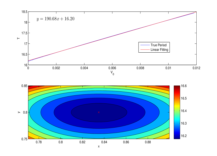
Figure 2: Up: values of $T$ as a function of $V$. Down: Contour lines with values of $T$ in a subset of $D$. Parameters set at $(\alpha,\gamma,\nu,\phi_{0},\phi_{1})=(0.025,0.055,3,0.040064,0.000064)$. Equilibrium point at $(\hat{x},\hat{y})=(0.8350,0.80)$.

Assumption 5.

Let $\sigma~{}:~{}y\in[0,1]\mapsto\sigma_{0}(1-y)$ with $\sigma_{0}>0$.

If we implicitly assume that the perturbation of the average growth rate $\alpha$ of the productivity is due to the flow of workers coming in and out of the fraction $y_{t}$ employed at time $t$, Assumption 5 conveniently expresses that this perturbation decreases with the employment rate since higher employment implies lower perturbation on the constant average rate $\alpha_{t}$. Other models can of course be considered.

Assumption 5 together with Assumption 4, and comparing with (25), satisfy Assumption 3. Indeed for all $y\in(0,1)$,

$$\sigma^{2}(y)\Phi^{\prime}(y)=\frac{2\sigma_{0}^{2}\phi_{1}}{(1-y)}\leq 2\sigma_{0}^{2}\left(V_{2}(y)-\phi_{1}\left(\frac{1}{1-\hat{y}}\left(\hat{y}\log(\hat{y})-\frac{1}{\hat{y}}\right)+\log(1-\hat{y})\right)\right)$$ (26)

and along with the sub-linearity of the log function,

$$-\kappa(x)-x\kappa^{\prime}(x)=\frac{2x-1}{\nu}\leq\frac{2}{1-\hat{x}}\left(V_{1}(x)+\hat{x}-\hat{x}\log(\hat{x})\right)\;.$$ (27)

In line with Assumptions 1 and 3 the vertical asymptote at $y=1$ implies that $\sigma^{2}(y)\Phi(y)\leq K_{0}V_{2}(y)+k_{0}$ for some $K_{0},k_{0}\in\mathbb{R}_{+}^{2}$. Under Assumption 3 and following (26) and (27), $K_{0}=0$ and $k_{0}=\sigma_{0}^{2}(\phi_{1}+\phi_{0})$.

Assumption 5 also implies that $(1-\tilde{y})^{2}$ is the root of a quadratic polynomial $\sigma_{0}^{2}(1-\tilde{y})^{4}-(\alpha+\phi_{0})(1-\tilde{y})^{2}+\phi_{1}=0\;.$ The latter shall have a unique root in $(0,1)$ to satisfy Assumption 6. The following example of condition is sufficient.

Assumption 6.

We assume $\phi_{1}\leq(\alpha+\phi_{0})/2$ and $\sigma_{0}\leq\max\{(\alpha+\phi_{0})/(2\sqrt{\phi_{1}}),(\alpha+\phi_{0}-\phi_{1})\}$.

We are now able to claim the existence of $K,k\in\mathbb{R}^{2}_{+}$ such that $|R(V_{0},\rho)|\leq K(V_{0}+\rho)+k$, where $R$ is defined in Proposition 4. A direct application provides

$$R(V_{0},\rho):=\max\limits_{D(V_{0},\rho)}\left\{\sigma_{0}^{2}(1-y)^{2}\left(\frac{2x-\hat{x}}{\nu}+\frac{2\phi_{1}y}{(1-y)^{3}}+\frac{\phi_{1}}{(1-y)^{2}}-\frac{\phi_{1}}{(1-\hat{y})^{2}}\right)\right\}.$$

Using (27), this estimate becomes $|R(V_{0},\rho)|\leq K(V_{0}+\rho)+k$ where $K:=(2\sigma_{0}^{2})/(1-\hat{x})$ and $k$ is an explicitly calculable constant. Following the same procedure with (26), $I(V_{0},\rho)\leq K(V_{0}+\rho)^{2}+k^{\prime}$ with the same $K$ and $k^{\prime}\neq k$. Now choosing $\mu=(\rho-(K(V_{0}+\rho)+k)\theta/2)/\sqrt{\theta}$ for some $\theta\geq 0$, so that $\Theta(\rho)=\theta$, Proposition 4 provides

$$\mathbb{P}\left[{\tau_{\rho}>\theta}\right]\geq\left(1-\frac{(K(V_{0}+\rho)^{2}+k^{\prime})\theta}{\left(\frac{1}{2}(K(V_{0}+\rho)+k)\theta-\rho\right)^{2}}\right)\;.$$

Theorem 5 is a straightly observable phenomenon with simulations, see Fig. 3. Under the assumptions of this section, the system has been simulated using XPPAUT with a fourth order Runge-Kutta scheme for the deterministic part, and an Euler scheme for the Brownian part. Fig. 3 illustrates the effect of the volatility level $\sigma_{0}$ on trajectories of the system, as for the economic quantity $P_{t}:=a_{t}y_{t}N_{t}$.

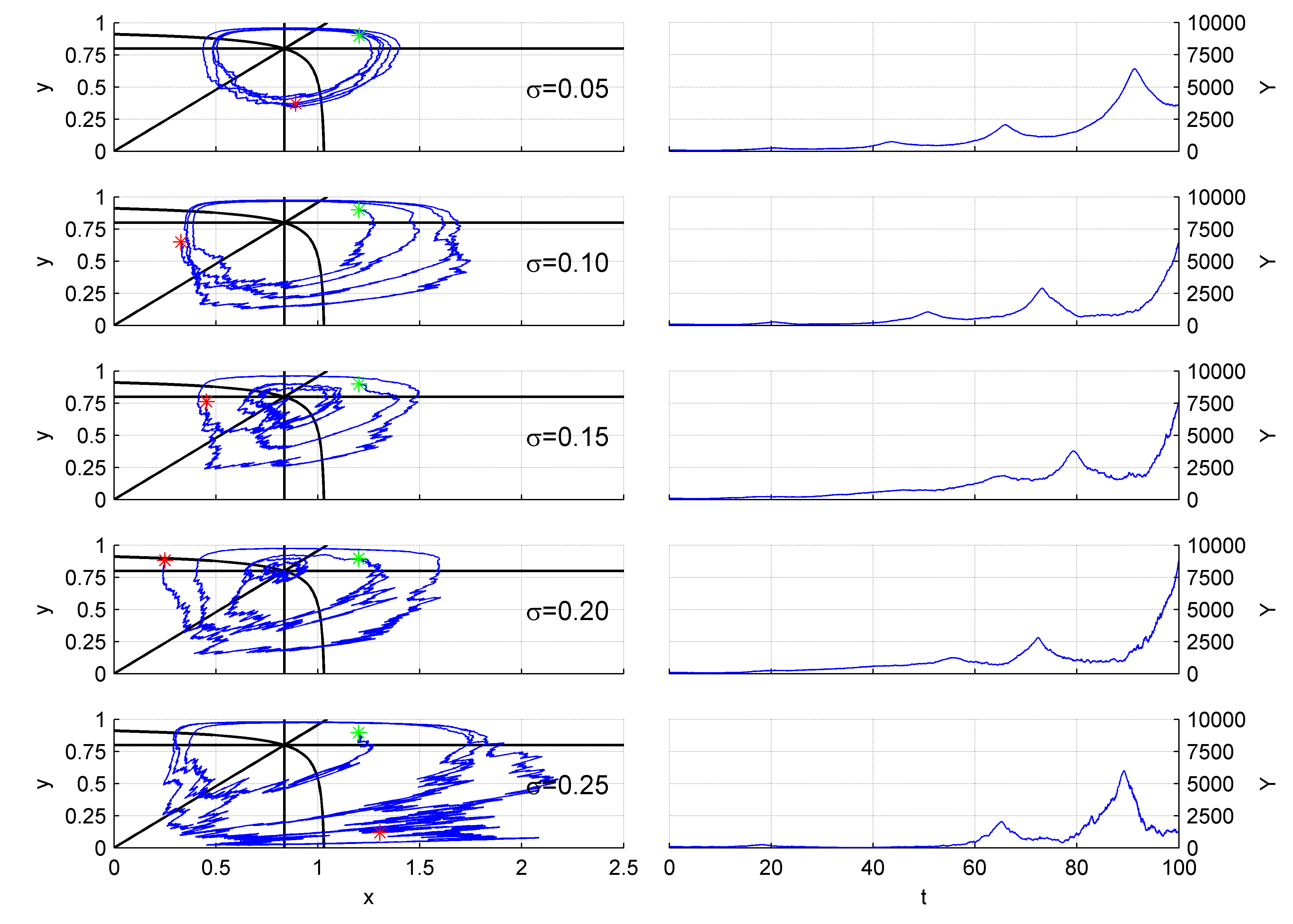
Figure 3: Left column : phase diagram $(x,y)$ of subsample paths of trajectories for (2) with different values of volatility $\sigma_{0}$, starting from the green star and stopping at the red start. Right column: evolution of output $P_{t}$ over time for the subsample path.

Apart from specific subregions of $D$ as $R_{1}$ or $R_{5}$ where Corollary 3.2 in [17] can provide an estimate for the expectation of the exit time, a bound for the expected period $\mathbb{E}\left[S\right]$ seems out of reach. Numerical simulations have nevertheless always provide reasonnable finite periods of stochastic orbits of (2). We thus expect that $\mathbb{E}\left[S\right]$ is finite for a wide range of values of $(x_{0},y_{0})\in D$. Let us start with $(x_{0},y_{0})\in R_{1}\cap R_{8}$ and reformulate $S$ of Definition 2 as the time the process crosses the line $y=\hat{\theta}x$ for the second time. This is equivalent to take $(x_{0},y_{0})\in R_{4}\cap R_{5}$. Resorting to numerical methods, we have simulated the system $2000$ times for $100$ different starting points in $R_{1}\cap R_{8}$ and recorded the position at the time when this line is crossed the second time, that is the positions after a full loop. Fig. 4 contains such examination for an array of values of $\sigma_{0}$. The expected time $\mathbb{E}\left[S\right]$ to complete a full-loop is also illustrated. As observed, there seems to be a stable attractive fixed point to $y_{0}\mapsto\mathbb{E}\left[y_{S}\right]$ for sufficiently large values of $\sigma_{0}$. If the starting point is picked too close to $(\hat{x},\hat{y})$, the expected crossing value after one loop is further away from it. On the other hand, if the one starts extremely far away from $(\hat{x},\hat{y})$, say with $y_{0}<0.25$, then the expected value after on loop is higher. This implies that after many loops, the expectation converges, and so does $\mathbb{E}\left[S\right]$ with the number of loops around $(\tilde{x},\tilde{y})$. Assuming that $\mathbb{E}\left[S\right]<+\infty$ for enough initial points, Theorem 6 can be used with $V$ at points $(0,0)$ and $(\tilde{x},\tilde{y})$ to prove the following conjecture.

Conjecture 1.

Consider the function ${\cal S}~{}:~{}y\in(0,\tilde{y})\mapsto\mathbb{E}\left[y_{S}\right]\in(0,\tilde{y})$ such that $(x_{t},y_{t})$ is a solution to (2) with $(x_{0},y_{0})=(y/\tilde{\theta},y)$, and $S$ is the finite stopping time defined by Theorem 5. Then ${\cal S}$ has at least one fixed point in $(0,\tilde{y})$.

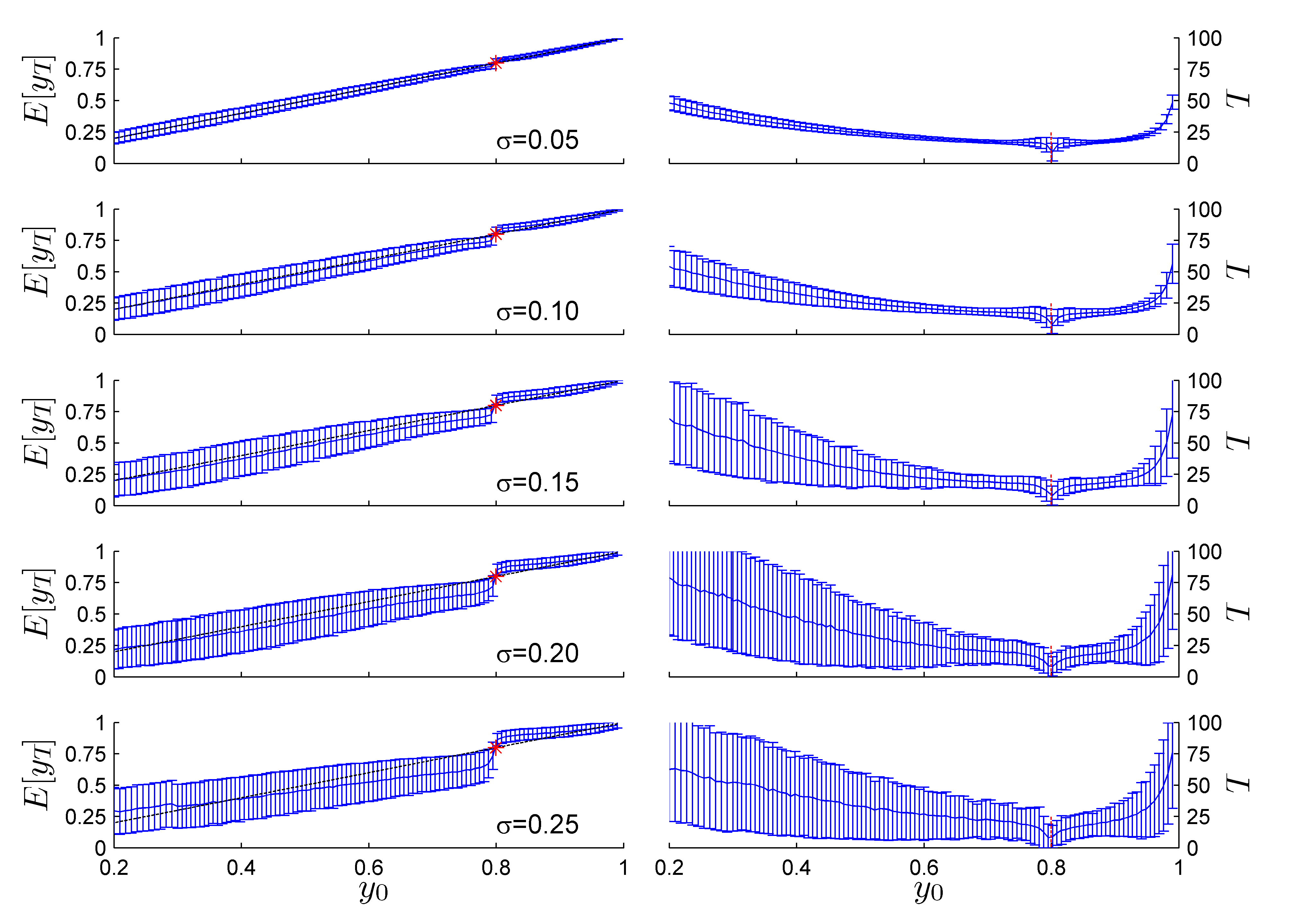
Figure 4: Expected values of employment $y$ after one full loop $y_{T}$ (left), and expected elapsed time $T$ (right). Computation performed in MATLAB, with $2000$ simulations for every value single one of the $100$ initial values taken along the line $y=\hat{\theta}x$.

6 Concluding remarks

This contribution attempts to draw the attention of dynamical system analysis onto macroeconomic models. Before looking into complex models of finance and crises, e.g. [5, 11, 15], we focus here on a Brownian perturbation added into a non-linear version of the Lotka-Volterra system used in Economics, the Goodwin model. To begin with, we recall the usual results for the deterministic planar oscillator: we provide the constant Entropy function and describe the period of the closed orbits drawned by the system. We then provide sufficient conditions for the stochastically perturbed system to stay in the meaningful domain $D$ which is a a bounded subset of $\mathbb{R}^{2}_{+}$ for the $y$-component. The entropy function is actually of great use for the last result, additionally to prior estimates on variations of the system.

We finally prove what seems a fundamental and staightforward property of the system, namely that a solution $(x_{t},y_{t})$ rotates with perturbations around a unique point $(\tilde{x},\tilde{y})$. The definition of stochastic orbits provided here conventienly suits the intuition of how the deterministic concept can be extended. However it has clearly not the ambition to be a definitive concept and further investigations might confirm its usefulness or its precarity. The proof exploits the concept of reccurent domains in an intensive manner.

We expect that economists seek interest in (2), as other perturbed macroeconomic systems (e.g. [16, 23]), for the possibility to adjust the model to observed past data (e.g. [1] and [13, 22]) and find a possible synthetic explanation for perturbations of business cycles (see [7, 12]).

References

- [1] M. Arató, A famous nonlinear stochastic equation (Lotka-Volterra model with diffusion), Mathematical and Computer Modelling, 38.7 (2003), 709–726.
- [2] A. Bahar and X. Mao, Stochastic delay Lotka–Volterra model, Journal of Mathematical Analysis and Applications, 292.2 (2004), 364–380.
- [3] S.M. Bartlett, On theoretical models for competitive and predatory biological systems, Biometrika, 44.1 (1957), 27–42.
- [4] G.Q. Cai and Y. K. Lin. Stochastic analysis of the Lotka-Volterra model for ecosystems, Physical Review E, 70.4 (2004), 041910.
- [5] B. Costa-Lima, M. R. Grasselli, X. S. Wangb and J. Wub, Destabilizing a stable crisis: employment persistence and government intervention in macroeconomics, to appear in Structural Change and Economic Dynamics, 2014.
- [6] M. Desai, B. Henry, A. Mosley and M. Pemberton, A clarification of the Goodwin model of the growth cycle, Journal of Economic Dynamics and Control, 30.12 (2006), 2661–2670.
- [7] C.L. Evans, (1992). Productivity shocks and real business cycles, Journal of Monetary Economics, 29.2 (1992), 191–208.
- [8] P. Flaschel, Some stability properties of Goodwin’s growth cycle a critical elaboration, Journal of Economics, 44.1 (1984), 63–69.
- [9] J. Glombowski and M. Krüger, Generalizations of Goodwin’s growth cycle model, Univ., FB Sozialwiss., 1986.
- [10] R.M. Goodwin, A growth cycle, Socialism, capitalism and economic growth (1967), 54–58.
- [11] M.R. Grasselli and B. Costa Lima, An analysis of the Keen model for credit expansion, asset price bubbles and financial fragility, Mathematics and Financial Economics, 6.3 (2012), 191–210.
- [12] G. D. Hansen, Indivisible labor and the business cycle, Journal of monetary Economics, 16.3 (1985), 309–327.
- [13] D. Harvie, Testing Goodwin: growth cycles in ten OECD countries, Cambridge Journal of Economics, 24.3 (2000), 349–376.
- [14] S.B. Hsu, A remark on the period of the periodic solution in the Lotka-Volterra system, Journal of Mathematical Analysis and Applications, 95.2 (1983), 428–436.
- [15] S. Keen, Finance and economic breakdown: modeling Minsky’s financial instability hypothesis, Journal of Post Keynesian Economics, 17.4 (1995), 607–635.
- [16] E. Kiernan and D.B. Madan, Stochastic stability in macro models, Economica (1989), 97–108.
- [17] R.Z. Khasminskii, Stochastic stability of differential equations, 2nd Ed. (Springerverlag Berlin Heidelberg), 2012.
- [18] R.Z. Khasminskii and F.C. Klebaner, Long term behavior of solutions of the Lotka-Volterra system under small random perturbations, The Annals of Applied Probability, 11.3 (2001), 952–963.
- [19] M. Liu and K. Wang, Stochastic Lotka–Volterra systems with Lévy noise, Journal of Mathematical Analysis and Applications, 410.2 (2014), 750–763.
- [20] X. Mao, G. Marion G. and E. Renshaw, Environmental Brownian noise suppresses explosions in population dynamics, Stochastic Processes and Their Applications, 97.1 (2002), 95–110.
- [21] X. Mao, S. Sabanis and E. Renshaw, Asymptotic behaviour of the stochastic Lotka-Volterra model, Journal of Mathematical Analysis and Applications, 287.1 (2003), 141–156.
- [22] S. Mohun and R. Veneziani, Goodwin cycles and the US economy, 1948-2004, 2006.
- [23] M. Neamtu, G. Mircea, M. Pirtea and D. Opris, The study of some stochastic macroeconomic models, Proceedings of the 11th WSEAS international conference on Applied Computer and Applied Computational Science (2012), 172–177.
- [24] D. Nguyen Huu and S. Vu Hai, Dynamics of a stochastic Lotka-Volterra model perturbed by white noise, Journal of mathematical analysis and applications, 324.1 (2006), 82–97.
- [25] T. Reichenbach, M. Mobilia, and E. Frey, Coexistence versus extinction in the stochastic cyclic Lotka-Volterra model, Physical Review E, 74.5 (2006), 051907.
- [26] J.G. Simmonds, J.G. A first look at perturbation theory, Courier Dover Publications, 1998.
- [27] U.H. Thygesen, U. H. (1997). A survey of Lyapunov techniques for stochastic differential equations, IMM, Department of Mathematical Modeling, Technical University of Denmark, working paper, 1997. Available at http://www.imm.dtu.dk
- [28] K. Velupillai, Some stability properties of Goodwin’s growth cycle, Journal of Economics, 39.3 (1979), 245–257.
- [29] R. Veneziani and S. Mohun, Structural stability and Goodwin’s growth cycle, Structural Change and Economic Dynamics, 17.4 (2006), 437–451.
- [30] C. Zhu and G. Yin, On competitive Lotka-Volterra model in random environments, Journal of Mathematical Analysis and Applications, 357.1 (2009), 154–170.
- [31] C. Zhu and G. Yin, On hybrid competitive Lotka-Volterra ecosystems, Nonlinear Analysis: Theory, Methods & Applications, 71.12 (2009), e1370–e1379.