splittheorem[1]

Theorem 0.1.

Proof.

In Section LABEL:prf:#1.∎

splitlemma[1]

Lemma 0.2.

Proof.

In Section LABEL:prf:#1.∎

splitcorollary[1]

Corollary 0.3.

Proof.

In Section LABEL:prf:#1.∎

splitproof

[-1cm]-3cm

STOCHASTIC OPTIMIZATION FOR MACHINE LEARNING

by

ANDREW COTTER

A thesis submitted in partial fulfillment of the requirements for the degree of

Doctor of Philosophy in Computer Science

at the

TOYOTA TECHNOLOGICAL INSTITUTE AT CHICAGO

Chicago, Illinois

August, 2013

Thesis committee:

Yury Makarychev

David McAllester

Nathan Srebro (thesis advisor)

Stephen Wright

Andrew Cotter: Stochastic Optimization for Machine Learning, © August, 2013

Abstract.1Abstract.1AbstractAbstractAbstract.1

Abstract

It has been found that stochastic algorithms often find good solutions much more rapidly than inherently-batch approaches. Indeed, a very useful rule of thumb is that often, when solving a machine learning problem, an iterative technique which relies on performing a very large number of relatively-inexpensive updates will often outperform one which performs a smaller number of much "smarter" but computationally-expensive updates.

In this thesis, we will consider the application of stochastic algorithms to two of the most important machine learning problems. Part i is concerned with the supervised problem of binary classification using kernelized linear classifiers, for which the data have labels belonging to exactly two classes (e.g. "has cancer" or "doesn’t have cancer"), and the learning problem is to find a linear classifier which is best at predicting the label. In Part ii, we will consider the unsupervised problem of Principal Component Analysis, for which the learning task is to find the directions which contain most of the variance of the data distribution.

Our goal is to present stochastic algorithms for both problems which are, above all, practical–they work well on real-world data, in some cases better than all known competing algorithms. A secondary, but still very important, goal is to derive theoretical bounds on the performance of these algorithms which are at least competitive with, and often better than, those known for other approaches.

Collaborators:

The work presented in this thesis was performed jointly with Raman Arora, Karen Livescu, Shai Shalev-Shwartz and Nathan Srebro.

STOCHASTIC OPTIMIZATION FOR MACHINE LEARNING

A thesis presented by

ANDREW COTTER

in partial fulfillment of the requirements for the degree of

Doctor of Philosophy in Computer Science.

Toyota Technological Institute at Chicago

Chicago, Illinois

August, 2013

Yury Makarychev
Committee member		Signature
David McAllester
Committee member		Signature
Chief academic officer
Nathan Srebro
Committee member		Signature
Thesis advisor
Stephen Wright
Committee member		Signature

July 19, 2013

Acknowledgments.1Acknowledgments.1AcknowledgmentsAcknowledgmentsAcknowledgments.1

Think not, is my eleventh commandment; and sleep when you can, is my twelfth.

— Herman Melville [38]

Part I   Support Vector Machines

Prior Work

1   Overview

One of the oldest and simplest problems in machine learning is that of supervised binary classification, in which the goal is, given a set of training vectors $x_{1},\dots,x_{n}\in\mathcal{X}$ with corresponding labels $y_{1},\dots,y_{n}\in\{\pm 1\}$ drawn i.i.d. from an unknown distribution $\mathcal{D}$, to learn a classification function which assigns labels to previously-unseen samples.

In this and the following chapters, we will consider the application of Support Vector Machines (SVMs) [9] to such problems. It’s important to clearly distinguish the problem to be solved (in this case, binary classification) from the tool used to solve it (SVMs). In the years since their introduction, the use of SVMs has become widespread, and it would not be unfair to say that it is one of a handful of canonical machine learning techniques with which nearly every student is familiar and nearly every practitioner has used. For this reason, it has become increasingly easy to put the cart before the horse, so to speak, and to view each advancement as improving the performance of SVMs, and not finding better binary classifiers.

This is not merely a semantic distinction, since practitioners must measure the performance of the classifiers which they find, while theoreticians often seek to bound the amount of computation required to find (and/or use) a good classifier. For both of these tasks, one requires a metric, a quantifiable way of answering the question “just how good is this classifier, anyway?”. For a SVM, which as we will see in Section 2 can be reduced to a convex optimization problem (indeed, there are several different such reductions in widespread use), the most convenient measure is often the suboptimality of the solution. This convenience is an illusion, however, since unless one has a means of converting a bound on suboptimality into a bound on the classification error on unseen data, this “suboptimality metric” will tell you nothing at all about the true quality of the solution.

Instead, we follow Bottou and Bousquet [5], Shalev-Shwartz and Srebro [51], and consider the “quality” of a SVM solution to be the expected proportion (with respect to $\mathcal{D}$) of classification mistakes made by the classifier, also known as the generalization error. The use of generalization error is hardly novel, neither in this thesis nor in the cited papers—rather, both seek to reverse the trend of viewing SVMs not as a means to an end, but as an end in themselves.

Having discussed the “how” and “why” of measuring the performance of SVMs, let us move on to the “what”. Any supervised learning technique consists of (at least) two phases: training and testing. In the training phase, one uses the set of provided labeled examples (the training data) to find a classifier. In the testing phase, one uses this classifier on previously-unseen data. Ideally, this “use” would be the application of the learned classifier in a production system—say, to provide targeted advertisements to web-page viewers. In research, evaluation of true production systems is rare. Instead, one simulates such an application by using the learned classifier to predict the labels of a set of held-out testing data, the true labels of which are known to the researcher, and then comparing the predicted labels to the true labels in order to estimate the generalization error of the classifier.

Most work focuses on finding a classifier which generalizes well as quickly as possible, i.e. jointly minimizing both the testing error and training runtime. In Chapter 2, a kernel SVM optimization algorithm will be presented which enjoys the best known bound, measured in these terms. Testing runtime should not be neglected, however. Indeed, in some applications, it may be far more important than the training runtime—for example, if one wishes to use a SVM for face recognition on a camera, then one might not mind a training runtime of weeks on a cluster, so long as evaluating the eventual solution on the camera’s processor is sufficiently fast. In Chapter 3, an algorithm for improving the testing performance of kernel SVMs will be presented, which again enjoys the best known bound on its performance.

The remainder of this chapter will be devoted to laying the necessary groundwork for the presentation of these algorithms. In Section 2, the SVM problem will be discussed in detail. In Section 3, generalization bounds will be introduced, and a key result enabling their derivation will be given. The chapter will conclude, in Sections 4 and 5, with discussions of several alternative SVM optimization algorithms, including proofs of generalization bounds.

2   Objective

	Definition	Name
$\mathcal{D}$		Data distribution
$n\in\mathbb{N}$		Training size
$x_{1},\dots,x_{n}\in\mathcal{X}$		Training vectors
$y_{1},\dots,y_{n}\in\{\pm 1\}$		Training labels
$\Phi:\mathcal{X}\rightarrow\mathcal{H}$		Kernel map
$K:\mathcal{X}\times\mathcal{X}\rightarrow\mathbb{R}$	$K(x,x^{\prime})=\left\langle{\Phi(x)},{\Phi(x^{\prime})}\right\rangle$	Kernel function such that $K(x,x)\leq 1$
$g_{w}:\mathcal{X}\rightarrow\mathbb{R}$	$g_{w}(x)=\left\langle{w},{\Phi(x)}\right\rangle$	Linear classifier
$g_{w,b}:\mathcal{X}\rightarrow\mathbb{R}$	$g_{w,b}(x)=\left\langle{w},{\Phi(x)}\right\rangle+b$	Linear classifier with bias
$c_{1},\dots,c_{n}\in\mathbb{R}$	$c_{i}=y_{i}\left\langle{w},{\Phi(x_{i})}\right\rangle$	Training responses
$\ell_{\mathrm{0/1}}:\mathbb{R}\rightarrow\mathbb{R}$	$\ell_{\mathrm{0/1}}(z)=\mathbf{1}_{\left\{z\leq 0\right\}}\left(z\right)$	Zero-one loss
$\ell_{\mathrm{hinge}}:\mathbb{R}\rightarrow\mathbb{R}$	$\ell_{\mathrm{hinge}}(z)=\max(0,1-z)$	Hinge loss
$\hat{\mathcal{L}}:(\mathcal{X}\rightarrow\mathbb{R})\rightarrow\mathbb{R}$	$\hat{\mathcal{L}}\left(g\right)=\frac{1}{n}\sum_{i=1}^{n}\ell\left(y_{i}g(x_{i})\right)$	Empirical loss
$\mathcal{L}:(\mathcal{X}\rightarrow\mathbb{R})\rightarrow\mathbb{R}$	$\mathcal{L}\left(g\right)=\mathbb{E}_{x,y\sim\mathcal{D}}\left[\ell\left(yg(x)\right)\right]$	Expected loss

Table 1.1: Summary of common notation across Chapters 1, 2 and 3. The training responses $c$ are calculated and kept up-to-date during optimization, so the $w$ parameterizing them should be taken to be the weight vector at the current optimization step—see Section 4 for details. The empirical and expected losses are generally subscripted with the particular loss which they use—for example, $\hat{\mathcal{L}}_{\mathrm{hinge}}\left(g_{w}\right)$ is the empirical hinge loss of the linear classifier defined by $w\in\mathcal{H}$.

Training a SVM amounts to finding a vector $w$ defining a classifier $x\mapsto\operatorname{sign}(\left\langle{w},{\Phi\left(x\right)}\right\rangle)$, that on the one hand has low norm, and on the other has a small training error, as measured through the average hinge loss on the training sample (see the definition of $\hat{\mathcal{L}}_{\mathrm{hinge}}\left(w\right)$ in Table 1.1). This is captured by the following bi-criterion optimization problem [25]:

$$\mbox{minimize}: \left\lVert{w}\right\rVert,\hat{\mathcal{L}}_{\mathrm{hinge}}\left(g_{w}\right)$$ (1.1)

We focus on kernelized SVMs, for which we assume the existence of a function $\Phi:\mathcal{X}\rightarrow\mathcal{H}$ which maps elements of $\mathcal{X}$ to elements of a kernel Hilbert space in which the “real” work will be done. The linear classifier which we seek is an element of this Hilbert space, and is therefore linear, not with respect to $\mathcal{X}$, but rather with respect to $\mathcal{H}$. It turns out that we can work in a Hilbert space $\mathcal{H}$ which is defined implicitly, via a kernel function $K(x,x^{\prime})=\left\langle{\Phi(x)},{\Phi(x^{\prime})}\right\rangle$, in which case we never need to evaluate $\Phi$, nor do we need to explicitly represent elements of $\mathcal{H}$. This can be accomplished by appealing to the representor theorem, which enables us to write $w$ as a linear combination of the training vectors with coefficients $\alpha$:

$$w=\sum_{i=1}^{n}\alpha_{i}y_{i}\Phi(x_{i})$$ (1.2)

It follows from this representation that we can write some important quantities in terms of only kernel functions, without explicitly using $\Phi$:

$$\left\lVert{w}\right\rVert^{2}= \sum_{i=1}^{n}\sum_{j=1}^{n}\alpha_{i}\alpha_{j}y_{i}y_{j}K(x_{i},x_{j})$$

$$\left\langle{w},{\Phi(x)}\right\rangle= \sum_{i=1}^{n}\alpha_{i}y_{i}K(x_{i},x)$$

These equations can be simplified further by making use of what we call the responses (see Table 1.1—more on these later). In the so-called “linear” setting, it is assumed that $\mathcal{X}=\mathcal{H}=\mathbb{R}^{d}$, and that $\Phi$ is the identity function. In this case, $K(x,x^{\prime})=\left\langle{x},{x^{\prime}}\right\rangle$, and kernel inner products are nothing but Euclidean inner products on $\mathcal{X}$. It is generally simpler to understand SVM optimization algorithms in the linear setting, with the kernel “extension” only being given once the underlying linear algorithm is understood. Here, we will attempt to do the next best thing, and will generally present our results explicitly, using $\Phi$ instead of $K$, referring to the kernel only when needed.

When first encountering the formulation of Problem 1.1, two questions naturally spring to mind: “why use the hinge loss?” and “why seek a low-norm solution?”. The answer to the second question is related to the first, so let us first discuss the use of the hinge loss. As was mentioned in the previous section, the underlying problem which we wish to solve is binary classification, which would naturally indicate that we should seek to find a classifier which makes the smallest possible number of mistakes on the training set—in other words, we should seek to minimize the training zero-one loss. Unfortunately, doing so is not practical, except for extremely small problem instances, because the underlying optimization problem is combinatorial in nature. There is, however, a class of optimization problems which are widely-studied, and known to be relatively easy to solve: convex optimization problems. Use of the hinge loss, which is a convex upper-bound on the zero-one loss, can therefore be justified by the fact that it results in a convex optimization problem, which we can then solve efficiently. In other words, we are approximating what we “really want to do”, for the sake of practicality.

This is, however, only a partial answer. While the hinge loss is indeed a convex upper bound on the zero-one loss, it is far from the only one, and others (such as the log loss) are in widespread use. Another more subtle but ultimately more satisfying reason for using the hinge loss relates to the fact that we want a solution which experiences low generalization error, coupled with the observation that a solution which performs well on the training set does not necessarily perform well with respect to the underlying data distribution. In the realizable case (i.e. where there exists a linear classifier which performs perfectly with respect to the underlying data distribution $\mathcal{D}$), the classification boundary of a perfect linear classifier must lie somewhere between the set of positive and negative training instances, so, in order to maximize the chance of getting it nearly-“right”, it only makes sense for a learning algorithm to place it in the middle. This intuition can be formalized, and it turns out that large-margin predictors (i.e. predictors for which all training elements of both classes are “far” from the classification boundary) do indeed tend to generalize well. When applying a SVM to a realizable problem, the empirical hinge loss will be zero provided that each training vector is at least $1/\left\lVert{w}\right\rVert$-far from the boundary, so minimizing the norm of $w$ is equivalent to maximizing the margin of the classifier. SVMs, which may also be applied to non-realizable problems, can therefore be interpreted as extending the idea of searching for large-margin classifiers to the case in which the data are not necessarily linearly separable, and we should therefore suspect that SVM solutions will tend to generalize well. This will be formalized in Section 3.

2.1   Primal Objective

A typical way in which Problem 1.1 is “scalarized” (i.e. transformed from a bi-criterion objective into a single unified objective taking an additional parameter) is the following:

$$\mbox{minimize}: \frac{\lambda}{2}\left\lVert{w}\right\rVert^{2}+\hat{\mathcal{L}}_{\mathrm{hinge}}\left(g_{w}\right)$$ (1.3)

Here, the parameter $\lambda$ controls the tradeoff between the norm (inverse margin) and the empirical error. Different values of $\lambda$ correspond to different Pareto optimal solutions of Problem 1.1, and the entire Pareto front can be explored by varying $\lambda$. We will refer to this as the “regularized objective”.

Alternatively, one could scalarize Problem 1.1 not by introducing a regularization parameter $\lambda$, but instead by enforcing a bound $R$ on the magnitude of $w$, and minimizing the empirical hinge loss subject to this constraint:

$$\mbox{minimize}: \hat{\mathcal{L}}_{\mathrm{hinge}}\left(g_{w}\right)$$ (1.4)

$$\mbox{subject to}: \left\lVert{w}\right\rVert\leq R$$

We will refer to this as the “norm-constrained objective”. It and the regularized objective are extremely similar. Like the regularized objective (while varying $\lambda$), varying $R$ causes optimal solutions to the norm-constrained objective to explore the Pareto frontier of Problem 1.1, so the two objectives are equivalent: for every choice of $\lambda$ in the regularized objective, there exists a choice of $R$ such that the optimal solution to the norm-constrained objective is the same as the optimal solution to the regularized objective, and vice-versa.

2.2   Dual Objective

Some SVM training algorithms, of which Pegasos [53] is a prime example, optimize the regularized objective directly. However, particularly for kernel SVM optimization, it is often more convenient to work on the Lagrangian dual of Problem 1.3:

$$\mbox{maximize}: \left\langle{\mathbf{1}},{\alpha}\right\rangle-\frac{1}{2}\left\lVert{w}\right\rVert^{2}$$ (1.5)

$$\mbox{subject to}: 0\leq\alpha_{i}\leq\frac{1}{\lambda n}$$

Here, as in Equation 1.2, $w=\sum_{i=1}^{n}\alpha_{i}y_{i}\Phi(x_{i})$, although now $\alpha$ is more properly considered not as the vector of coefficients resulting from application of the representor theorem, but rather the dual variables which result from taking the Lagrangian dual of Problem 1.3. Optimal solutions to the dual objective correspond to optimal solutions of the primal, and vice-versa. The most obvious practical difference between the two is that the dual objective is a quadratic programming problem subject to box constraints, and is thus particularly “easy” to solve efficiently, especially in comparison to the primal, which is not even smooth (due to the “hinge” in the hinge loss).

There is another more subtle difference, however. While optimal solutions to Problems 1.3 and 1.5 both, by varying $\lambda$, explore the same set of Pareto optimal solutions to Problem 1.1, these alternative objectives are decidedly not equivalent when one considers the quality of suboptimal solutions. We’ll illustrate this phenomenon with a trivial example.

Consider the one-element dataset $\left(x_{1},y_{1}\right)=\left(1,1\right)$ with $\mathcal{X}=\mathcal{H}=\mathbb{R}$ and $\Phi$ being the identity (i.e. this is a linear SVM), and suppose that we wish to optimize the regularized or dual objective with $\lambda=\frac{1}{2}$. For this dataset, both the weight vector $w$ and the vector of dual variables $\alpha$ are one-dimensional scalars, and the expression $w=\sum_{i=1}^{n}\alpha_{i}y_{i}x_{i}$ shows that $w=\alpha$. It is easy to verify that the optimum of both of these objectives occurs at $\hat{w}^{*}=\hat{\alpha}^{*}=1$.

For suboptimal solutions, however, the correspondence between the two objectives is less attractive. Consider, for example, suboptimal solutions of the form $w^{\prime}=\alpha^{\prime}=1-\delta$, and notice that these solutions are dual feasible for $0\leq\delta\leq 1$. The suboptimality of the dual objective function for this choice of $\alpha$ is given by:

$$\left(\hat{\alpha}^{*}-\frac{1}{2}\left(\hat{\alpha}^{*}\right)^{2}\right)-\left(\alpha^{\prime}-\frac{1}{2}\left(\alpha^{\prime}\right)^{2}\right)=\frac{1}{2}\delta^{2}$$

while the primal suboptimality for this choice of $w$ is:

$$\left(\frac{\lambda}{2}\left(w^{\prime}\right)^{2}+\max\left(0,1-w^{\prime}\right)\right)-\left(\frac{\lambda}{2}\left(\hat{w}^{*}\right)^{2}+\max\left(0,1-\hat{w}^{*}\right)\right)=\frac{1}{4}\delta^{2}+\frac{1}{2}\delta$$

In other words, $O(\epsilon)$-suboptimal solutions to the dual objective may be only $O(\sqrt{\epsilon})$-suboptimal in the primal. As a consequence, an algorithm which converges rapidly in the dual may not do so in the primal, and more importantly, may not do so in terms of the ultimate quantity of interest, generalization error. Hence, the apparent ease of optimizing the dual objective may not be as beneficial as it at first appears.

In Chapter 2, an algorithm will be developed based on a third equivalent formulation of the SVM problem, called the slack-constrained objective. The convergence rate of this algorithm, measured in terms of suboptimality, is unremarkable. Instead, it performs well because $\epsilon$-suboptimal solutions to the slack-constrained objective are better, in terms of known bounds on the generalization error, than $\epsilon$-suboptimal solutions to the other objectives mentioned in this section.

2.3   Unregularized Bias

Frequently, SVM problems contain an unregularized bias term—rather than the classification function being $g_{w}(x)=\left\langle{w},{\Phi(x)}\right\rangle$, with the underlying optimization problem searching for a good low-weight vector $w$, the classification function is taken to be the sign of $g_{w,b}(x)=\left\langle{w},{\Phi(x)}\right\rangle+b$, where $w$ is, as before, low-norm, but $b\in\mathbb{R}$ has no constraints on its magnitude. Intuitively, the difference is that, in the former case, the classification boundary is a hyperplane which passes through the origin (i.e. is a subspace of $\mathcal{H}$), while in the latter case it does not (i.e. it is an affine subspace).

The optimization problems which we have so far considered for SVMs do not contain a bias term, and in Chapters 2 and 3 our focus will be on such problems. This is purely to simplify the presentation, however—the algorithms introduced in these chapters can be extended to work on problems with an unregularized bias fairly easily.

Updating the objectives of Section 2.1 to include an unregularized bias amounts to nothing more than inserting $b$ into the hinge loss term. For example, the regularized objective of Problem 1.3 becomes:

$$\mbox{minimize}: \frac{\lambda}{2}\left\lVert{w}\right\rVert^{2}+\hat{\mathcal{L}}_{\mathrm{hinge}}\left(g_{w,b}\right)$$ (1.6)

Precisely the same substitution works on the norm-constrained objective of Problem 1.4.

Finding the Lagrangian dual of Problem 1.6 gives us the analogue of the dual objective of Problem 1.5

$$\mbox{maximize}: \left\langle{\mathbf{1}},{\alpha}\right\rangle-\frac{1}{2}\left\lVert{w}\right\rVert^{2}$$ (1.7)

$$\mbox{subject to}: 0\leq\alpha_{i}\leq\frac{1}{\lambda n},\ \ \sum_{i=1}^{n}y_{i}\alpha_{i}=0$$

The only difference here is the addition of the constraint $\sum_{i=1}^{n}y_{i}\alpha_{i}=0$. As before, we can derive $w$ from $\alpha$ via Equation 1.2, but finding $b$ is slightly more involved. For an optimal vector $\alpha$ of dual variables, it will be the case that $b=y_{i}-\left\langle{w},{\Phi(x_{i})}\right\rangle$ for any $i$ such that $0<\alpha_{i}<\nicefrac{{1}}{{\lambda n}}$ (i.e. $\alpha_{i}$ is bound to neither a lower nor upper-bound constraint), so the most common method for finding $b$ from a (not necessarily optimal) $\alpha$ is to solve this equation for all valid $i$, and average the results.

3   SVM Generalization Bounds

	Overall		$\epsilon=\Omega\left(L^{*}\right)$
	Training	Testing	Training	Testing
SGD on Problem 1.4	$\left(\frac{L^{*}+\epsilon}{\epsilon}\right)\frac{R^{4}}{\epsilon^{3}}$	$\frac{R^{2}}{\epsilon^{2}}$	$\frac{R^{4}}{\epsilon^{3}}$	$\frac{R^{2}}{\epsilon^{2}}$
Dual Decomposition	$\left(\frac{L^{*}+\epsilon}{\epsilon}\right)^{2}\frac{R^{4}}{\epsilon^{2}}$	$\left(\frac{L^{*}+\epsilon}{\epsilon}\right)\frac{R^{2}}{\epsilon}$	$\frac{R^{4}}{\epsilon^{2}}$	$\frac{R^{2}}{\epsilon}$
Perceptron + Online-to-Batch	$\left(\frac{L^{*}+\epsilon}{\epsilon}\right)^{3}\frac{R^{4}}{\epsilon}$	$\left(\frac{L^{*}+\epsilon}{\epsilon}\right)^{2}R^{2}$	$\frac{R^{4}}{\epsilon}$	$R^{2}$
Random Fourier Features	$\left(\frac{L^{*}+\epsilon}{\epsilon}\right)\frac{dR^{4}}{\epsilon^{3}}$	$\frac{dR^{2}}{\epsilon^{2}}$	$\frac{dR^{4}}{\epsilon^{3}}$	$\frac{dR^{2}}{\epsilon^{2}}$

Table 1.2: Summary of results from Sections 4 and 5. First three rows: upper bounds on the number of kernel evaluations required to train a kernelized classifier / evaluate a solution on a single previously-unseen example, such that $\mathcal{L}_{\mathrm{0/1}}\left(g_{w}\right)\leq L^{*}+\epsilon$. Last row: number of $d$-dimensional inner products (random Fourier feature constructions) required. All quantities are given up to constant and log factors, and hold with probability $1-\delta$ (although the dependence on $\delta$ is not shown in this table). It is assumed that $K(x,x)\leq 1$ with probability one for $x\sim\mathcal{D}$, and furthermore, in the last column, that $\mathcal{X}=\mathbb{R}^{d}$. The quantity $L^{*}$ can be read as the “optimal hinge loss”, and is the expected hinge loss (with respect to $\mathcal{D}$) suffered by an arbitrary reference classifier $g_{u}$ with $\left\lVert{u}\right\rVert\leq R$. For the last row, $\left\lVert{u}\right\rVert\leq\left\lVert{u}\right\rVert_{1}\leq R$, with the first inequality following from the fact that $K(x,x^{\prime})\leq 1$. The “Overall” columns show the standard optimistic bounds, while the “$\epsilon=\Omega\left(L^{*}\right)$” columns give versions of these bounds in the most typical machine learning setting, in which the desired level of suboptimality $\epsilon$ is comparable to the optimal hinge loss.

Before introducing and analyzing particular SVM optimization algorithms, we must first describe how these analyses will performed, and what the results of such analyses should be. In this section, we will give a bound on the sample size $n$ required to guarantee good generalization performance (in terms of the 0/1 loss) for a low-norm classifier which is $\epsilon$-suboptimal in terms of the empirical hinge loss. This bound (Lemma LABEL:lem:svm-introduction:generalization-from-expected-loss) essentially enables us to transform a bound on the empirical hinge loss into a bound on generalization performance. This lemma is a vital building block of the bounds derived in the following sections of this chapter (see Table 1.2), as well as in Chapters 2 and 3.

In order to simplify the presentation of our generalization bounds, throughout this chapter, as well as Chapters 2 and 3, we make the simplifying assumption that $K(x,x^{\prime})\leq 1$ with probability $1$ (with respect to the underlying data distribution $\mathcal{D}$).

lem:svm-introduction:generalization-from-expected-loss

Let $u$ be an arbitrary linear classifier, and suppose that we sample a training set of size $n$, with $n$ given by the following equation, for parameters $B\geq\left\lVert{u}\right\rVert$, $\epsilon>0$ and $\delta\in\left(0,1\right)$:

$$n=\tilde{O}\left(\left(\frac{\mathcal{L}_{\mathrm{hinge}}\left(g_{u}\right)+\epsilon}{\epsilon}\right)\frac{\left(B+\log\frac{1}{\delta}\right)^{2}}{\epsilon}\right)$$

Then, with probability $1-\delta$ over the i.i.d. training sample $x_{i},y_{i}:i\in\left\{1,\dots,n\right\}$, we have that $\hat{\mathcal{L}}_{\mathrm{hinge}}\left(g_{u}\right)\leq\mathcal{L}_{\mathrm{hinge}}\left(g_{u}\right)+\epsilon$ and $\mathcal{L}_{\mathrm{0/1}}\left(g_{w}\right)\leq\hat{\mathcal{L}}_{\mathrm{hinge}}\left(g_{u}\right)+\epsilon$, and in particular that $\mathcal{L}_{\mathrm{0/1}}\left(g_{w}\right)\leq\mathcal{L}_{\mathrm{hinge}}\left(g_{u}\right)+2\epsilon$ uniformly for all $w$ satisfying:

$$\left\lVert{w}\right\rVert\leq B,\ \ \hat{\mathcal{L}}_{\mathrm{hinge}}\left(g_{w}\right)\leq\hat{\mathcal{L}}_{\mathrm{hinge}}\left(g_{u}\right)+\epsilon$$

Lemma 1.16 gives that $\hat{\mathcal{L}}_{\mathrm{hinge}}\left(g_{w}\right)\leq\mathcal{L}_{\mathrm{hinge}}\left(u\right)+2\epsilon$ provided that Equation 1.17 is satisfied. Taking $L=\mathcal{L}_{\mathrm{hinge}}\left(u\right)+2\epsilon$ in Lemma 1.13 gives the desired result, provided that Equation 1.14 is also satisfied. Equation 1.18 is what results from combining these two bounds. The fact that this argument holds with probability $1-2\delta$, while our claim is stated with probability $1-\delta$, is due to the fact that scaling $\delta$ by $1/2$ only changes the bound by a constant.

The bounds which we derive from this Lemma are optimistic, in the sense that they will look like $n=O\left(\nicefrac{{1}}{{\epsilon^{2}}}\right)$ when the problem is difficult (i.e. $\epsilon$ is small relative to $\mathcal{L}_{\mathrm{hinge}}\left(g_{u}\right)$), and be better when the problem is easier, approaching $n=O\left(\nicefrac{{1}}{{\epsilon}}\right)$ when it is linearly separable (i.e. $\mathcal{L}_{\mathrm{hinge}}\left(g_{u}\right)=0$).

Applying Lemma LABEL:lem:svm-introduction:generalization-from-expected-loss to a particular algorithm follows two steps. First, we determine, on an algorithm-by-algorithm basis, what is required to find a solution $w$ which satisfies the following:

$$\left\lVert{w}\right\rVert\leq B,\ \ \hat{\mathcal{L}}_{\mathrm{hinge}}\left(g_{w}\right)\leq\hat{\mathcal{L}}_{\mathrm{hinge}}\left(g_{u}\right)+\epsilon$$

Here, $u$ is an arbitrary reference classifier with $\left\lVert{u}\right\rVert\leq B$ (typically, $u$ will be taken to be the optimum). Next, we use Lemma LABEL:lem:svm-introduction:generalization-from-expected-loss to find the sample size $n$ required such that $\mathcal{L}_{\mathrm{0/1}}\left(g_{w}\right)\leq\mathcal{L}_{\mathrm{hinge}}\left(g_{u}\right)+\epsilon$ is satisfied.

4   Traditional Optimization Algorithms

$\mbox{{optimize}}\left(n:\mathbb{N},d:\mathbb{N},x_{1},\dots,x_{n}:\mathbb{R}^{d},y_{1},\dots,y_{n}:\left\{\pm 1\right\},T:\mathbb{N},K:\mathbb{R}^{d}\times\mathbb{R}^{d}\rightarrow\mathbb{R}\right)$
1	$w:=0$;
2	$\mbox{{for }}t=1\mbox{{ to }}T$
3		Somehow choose a working set $\mathcal{I}\subseteq\{1,\dots,n\}$ of training indices;
4		Calculate the responses $c_{i}=y_{i}\left\langle{w},{\Phi\left(x_{i}\right)}\right\rangle$ and use them to optimize some
		subproblem on the working set $\mathcal{I}$;
5		Update $w$ by adding some linear combination of $\Phi\left(x_{i}\right):i\in\mathcal{I}$ to $w$;
6		Scale $w$ by multiplying it by some quantity $\gamma$;
7	$\mbox{{return }}w$;

Algorithm 1.3 Outline of a “traditional” SVM optimization algorithm. Different algorithms will do different things in the “some” portions.

In this section, algorithms for optimizing a SVM based on traditional convex optimization techniques will be described. One significant feature of many such algorithms is that they can be represented as instances of a common “outline”, in which a weight vector $w$ is found iteratively according to Algorithm 1.3. The various algorithms which we will consider in this section, as well as Chapters 2 and 3, differ in how they perform the “some” portions of this algorithm, but their presentation (and analysis, to some extent) will be simplified by recognizing them as instances of this outline. The existence of this general outline also has important consequences for the implementation of these algorithms, since it enables one to create an optimized shared implementation of those portions of the update which are identical across all traditional optimizers, with specialized code only being necessary for the small number of differences between them. ISSVM, which contains the reference implementations of the algorithms of Chapters 2 and 3, is a project designed according to these principles.

For a linear kernel, as was discussed in Section 2, $\Phi$ is the identity function, and one may implement a traditional optimizer by essentially following exactly Algorithm 1.3. For a kernelized SVM optimizer, however, we cannot explicitly depend on $\Phi$, and must instead appeal to Equation 1.2 to represent $w$ as a linear combination of $\Phi\left(x_{i}\right)$ with coefficients $\alpha_{i}$, which enables us to write the algorithm in terms of only the coefficients $\alpha$ and kernel evaluations.

$\mbox{{optimize}}\left(n:\mathbb{N},d:\mathbb{N},x_{1},\dots,x_{n}:\mathbb{R}^{d},y_{1},\dots,y_{n}:\left\{\pm 1\right\},T:\mathbb{N},K:\mathbb{R}^{d}\times\mathbb{R}^{d}\rightarrow\mathbb{R}\right)$
1	$\alpha:=0$; $c:=0$;
2	$\mbox{{for }}t=1\mbox{{ to }}T$
3		Somehow choose a working set $\mathcal{I}\subseteq\{1,\dots,n\}$ of training indices;
4		Optimize some subproblem on the working set $\mathcal{I}$;
5		Update $w$ by adding some $\delta_{i}$ to $\alpha_{i}$ for every $i\in\mathcal{I}$, and update the responses by
		adding $y_{i}y_{j}\delta_{i}K(x_{i},x_{j})$ to $c_{j}$ for every $i\in\mathcal{I}$ and $j\in\{1,\dots,n\}$;
6		Scale $w$ by multiplying $\alpha$ and $c$ by some quantity $\gamma$;
7	$\mbox{{return }}\alpha$;

Algorithm 1.4 Outline of a “traditional” SVM optimization algorithm in the kernel setting which keeps track of a complete up-to-date vector of $n$ responses throughout. Different algorithms will do different things in the “some” portions.

For all of the algorithms which we will consider, calculating the responses on line $4$ will be the most computationally expensive step, with a cost of $kn$ kernel evaluations, where $k=\left\lvert{\mathcal{I}}\right\rvert$ is the number of responses which we need to calculate. Alternatively, we can modify the algorithm to keep track of a complete vector of $n$ responses at all times, updating them whenever we make a change to $\alpha$—this is done in Algorithm 1.4. Updating the responses in line $5$ costs $kn$ kernel evaluations, as before. However, this version has the advantage that the complete vector of responses is available at every point. In particular, we can use $c$ to choose the working set $\mathcal{I}$ on line $3$.

The existence of this “improved” optimization outline demonstrates why the best linear SVM optimization algorithms tend to be different from the best kernel SVM algorithms. In the linear setting, calculating $k$ responses only costs $k$ inner products per iteration, while keeping a complete up-to-date vector $c$ would cost $n$ inner products per iteration. As a result, good algorithms tend to be “fast but dumb”, in that each iteration is computationally very inexpensive, but cannot include the use of advanced working-set-selection heuristics because the responses are unavailable (and computing them would lead to an unacceptable increase to the cost of each iteration). In the kernel setting, however, we must perform $kn$ kernel evaluations per iteration anyway, and therefore prefer “slower but smarter” updates, for two reasons. First, there is no additional cost for keeping a complete up-to-date vector of responses available throughout, which enables one to use a better working-set-selection heuristic; second, because every iteration is already fairly expensive (at least $O(kn)$ as opposed to $O(d)$ in the linear setting, where $\mathcal{X}=\mathbb{R}^{d}$), all of the steps of the update, most importantly the subproblem optimization, can be made more computationally expensive without increasing the asymptotic per-iteration cost of the algorithm.

The work described in this thesis focuses on the kernel setting, so the canonical optimization algorithm outline will be Algorithm 1.4. With this said, it is important to keep in mind that switching between the linear and kernel settings can dramatically change the performance profile of each algorithms under consideration. In particular, algorithms based on stochastic gradient descent (Section 4.1), as well as stochastic dual coordinate ascent (Section 4.2), which do not make use of the complete vector of responses when finding a working set, operate much more efficiently in the linear setting.

4.1   Stochastic Gradient Descent

Probably the simplest algorithm which can be applied to SVM optimization is stochastic gradient descent (SGD). We will present two SGD algorithms, the first being SGD applied to the norm-constrained SVM objective of Problem 1.4, and the second to the regularized objective of Problem 1.3. Due to the similarity of the objectives, the two optimization algorithms are almost the same, although, as we will see, the former enjoys a slightly superior convergence rate, despite the fact that the latter algorithm, also known as Pegasos [53], is far more well-known.

4.1.1   Norm-Constrained Objective

Formally differentiating the norm-constrained SVM objective (Problem 1.4—refer to the definition of the empirical hinge loss in Table 1.1) yields that:

$$\frac{\partial}{\partial w}=\frac{1}{n}\sum_{i=1}^{n}\mathbf{1}_{\left\{y_{i}\left\langle{w},{\Phi\left(x_{i}\right)}\right\rangle<1\right\}}\left(y_{i}\Phi\left(x_{i}\right)\right)$$

We could perform projected gradient descent (GD) by iteratively subtracting a multiple of the above quantity from $w$, and then projecting $w$ onto the feasible set $\left\{w:\left\lVert{w}\right\rVert\leq R\right\}$. This, however, would be an extremely computationally expensive update, because it requires knowledge of all $n$ values of the responses $c_{i}=y_{i}\left\langle{w},{\Phi\left(x_{i}\right)}\right\rangle$, and could potentially add a multiple of every training element to $w$ at each iteration. As a result, regardless of whether we calculate the responses only as-needed, or keep an up-to-date set of all of the responses, the cost of each iteration is potentially as high as $n^{2}$ kernel evaluations in the kernel setting.

It has been observed [65, 53, 51, 54] that performing a large number of simple updates generally leads to faster convergence than performing fewer computationally expensive (but “smarter”) updates, which motivates the idea of using SGD, instead of GD, by iteratively performing the following steps on the $t$th iteration:

1. Sample $i$ uniformly from $\{1,\dots,n\}$.

2. If $y_{i}\left\langle{w},{\Phi\left(x_{i}\right)}\right\rangle<1$ then subtract $\eta_{t}y_{i}\Phi\left(x_{i}\right)$ from $w$.

3. If $\left\lVert{w}\right\rVert>R$ then multiply $w$ by $R/\left\lVert{w}\right\rVert$.

Notice that the quantity added to $w$ in step 2 is equal in expectation (over $i$) to the gradient of the objective with respect to $w$, and therefore that this is a SGD algorithm. Furthermore, these three steps together constitute an instance of the “traditional” algorithm outline, showing that they can be performed using an efficient modular implementation of Algorithm 1.4. The following lemma gives the theoretical convergence rate of this algorithm, in the kernel setting:

thm:svm-introduction:norm-constrained-runtime

Let $u\in\mathcal{H}$ be an arbitrary reference classifier with $R\geq\left\lVert{u}\right\rVert$. Suppose that we perform $T$ iterations of SGD on the norm-constrained objective, with $w_{t}$ the weight vector after the $t$th iteration. If we define $\bar{w}=\frac{1}{T}\sum_{t=1}^{T}w_{t}$ as the average of these iterates, then there exist values of the training size $n$ and iteration count $T$ such that SGD on the norm-constrained objective with step size $\eta_{t}=R\sqrt{\nicefrac{{2}}{{t}}}$ finds a solution $\bar{w}=\sum_{i=1}^{n}\bar{\alpha}_{i}y_{i}\Phi\left(x_{i}\right)$ satisfying:

$$\mathcal{L}_{\mathrm{0/1}}\left(g_{\bar{w}}\right)\leq\mathcal{L}_{\mathrm{hinge}}\left(g_{u}\right)+\epsilon$$

after performing the following number of kernel evaluations:

$$\mbox{\#K}=\tilde{O}\left(\left(\frac{\mathcal{L}_{\mathrm{hinge}}\left(g_{u}\right)+\epsilon}{\epsilon}\right)\frac{R^{4}}{\epsilon^{3}}\log^{3}\frac{1}{\delta}\right)$$

with the size of the support set of $\bar{w}$ (the number nonzero elements in $\bar{\alpha}$) satisfying:

$$\mbox{\#S}=O\left(\frac{R^{2}}{\epsilon^{2}}\log\frac{1}{\delta}\right)$$

the above statements holding with probability $1-\delta$.

We may bound the online regret of SGD using Zinkevich [66, Theorem 1], which gives the following, if we let $i_{t}$ be the index sampled at the $t$th iteration:

$$\frac{1}{T}\sum_{t=1}^{T}\ell_{\mathrm{hinge}}\left(g_{w_{t}}\left(x_{i_{t}}\right)\right)\leq\frac{1}{T}\sum_{t=1}^{T}\ell_{\mathrm{hinge}}\left(g_{u}\left(x_{i_{t}}\right)\right)+R\sqrt{\frac{1}{2T}}$$

In order to change the above regret bound into a bound on the empirical hinge loss, we use the online-to-batch conversion of Cesa-Bianchi et al. [11, Theorem 1], which gives that with probability $1-\delta$:

$$\hat{\mathcal{L}}_{\mathrm{hinge}}\left(g_{\bar{w}}\right)\leq\hat{\mathcal{L}}_{\mathrm{hinge}}\left(g_{u}\right)+R\sqrt{\frac{1}{2T}}+R\sqrt{\frac{2}{T}\log\frac{1}{\delta}}$$

Which gives that $\bar{w}$ will be $\epsilon$-suboptimal after performing the following number of iterations:’

$$T=O\left(\frac{R^{2}}{\epsilon^{2}}\log\frac{1}{\delta}\right)$$

Because $w$ is projected onto the Euclidean ball of radius $R$ at the end of every iteration, we must have that $\left\lVert{\bar{w}}\right\rVert\leq R$, so we may apply Lemma LABEL:lem:svm-introduction:generalization-from-expected-loss to bound $n$ as (Equation 1.18):

$$n=\tilde{O}\left(\left(\frac{\mathcal{L}_{\mathrm{hinge}}\left(g_{u}\right)+\epsilon}{\epsilon}\right)\frac{\left(R+\log\frac{1}{\delta}\right)^{2}}{\epsilon}\right)$$

The number of kernel evaluations performed over $T$ iterations is $Tn$, and the support size is $T$, which gives the claimed result.

4.1.2   Regularized Objective

Applying SGD to the regularized objective results in a similar update, except that instead of explicitly projecting onto the feasible region, it is the regularization term of the objective which ensures that the weight vector $w$ does not become too large. Differentiating Problem 1.3 with respect to $w$ yields:

$$\frac{\partial}{\partial w}=\lambda w+\frac{1}{n}\sum_{i=1}^{n}\mathbf{1}_{\left\{y_{i}\left\langle{w},{\Phi\left(x_{i}\right)}\right\rangle<1\right\}}\left(y_{i}\Phi\left(x_{i}\right)\right)$$

Which shows that the following is a SGD update:

1. Sample $i$ uniformly from $\{1,\dots,n\}$.

2. Multiply $w$ by $1-\eta_{t}\lambda$.

3. If $y_{i}\left\langle{w},{\Phi\left(x_{i}\right)}\right\rangle<1$ then subtract $\eta_{t}y_{i}\Phi\left(x_{i}\right)$ from $w$.

With an appropriate choice of the step size $\eta_{t}$, this algorithm is known as Pegasos [53]. Here, steps $2$ and $3$ together add $\eta$ times $\lambda w+\mathbf{1}_{\left\{y_{i}\left\langle{w},{\Phi\left(x_{i}\right)}\right\rangle<1\right\}}\left(y_{i}\Phi\left(x_{i}\right)\right)$ to $w$, which is equal in expectation to the gradient of the regularized objective with respect to $w$. Once more, this is an instance of the “traditional” algorithm outline (except that the adding and scaling steps are swapped, which makes no difference).

The only difference between SGD on the norm-constrained and regularized objectives is that the first projects $w$ onto the Euclidean ball of radius $R$, while the second shrinks $w$ by a factor proportional to the step size at every iteration. At first glance, this is insignificant, but once we move on to analyzing the performance of these algorithms we find that there are, in fact, pronounced differences.

The first difference results from the fact that, when one applies SGD to non-strongly-convex objectives, the use of a step size $\eta_{t}\propto 1/\sqrt{t}$ typically yields the best convergence rates, whereas $\eta_{t}\propto 1/t$ is better for strongly-convex objectives. These two algorithms are not exceptions—the norm-constrained objective is not strongly convex, while the regularized objective is (with convexity parameter $\lambda$), and these two algorithms perform best, at least in theory, with $O(1/\sqrt{t})$ and $O(1/t)$ step sizes, respectively.

The second main difference is a result of our use of Lemma LABEL:lem:svm-introduction:generalization-from-expected-loss, which gives a bound on the generalization error suffered by weight vectors $w$ with some maximum norm $B$. Because this lemma is stated in terms of a norm-constrained weight vector, it is more convenient to apply it to the result of applying SGD to the norm-constrained objective. On the regularized objective, a bound on the norm of $w$ can only be derived from a bound on the suboptimality, which ultimately causes the convergence rate to not be quite as good as we would hope, as we can see in the following lemma:

thm:svm-introduction:regularized-runtime

Let $u\in\mathcal{H}$ be an arbitrary reference classifier. Suppose that we perform $T$ iterations of Pegasos, with $w_{t}$ the weight vector after the $t$th iteration. If we define $\bar{w}=\frac{1}{T}\sum_{t=1}^{T}w_{t}$ as the average of these iterates, then there exist values of the training size $n$, iteration count $T$ and regularization parameter $\lambda$ such that Pegasos with step size $\eta_{t}=\nicefrac{{1}}{{\lambda t}}$ finds a solution $\bar{w}=\sum_{i=1}^{n}\bar{\alpha}_{i}y_{i}\Phi\left(x_{i}\right)$ satisfying:

$$\mathcal{L}_{\mathrm{0/1}}\left(g_{w}\right)\leq\mathcal{L}_{\mathrm{hinge}}\left(g_{u}\right)+\epsilon$$

after performing the following number of kernel evaluations:

$$\mbox{\#K}=\tilde{O}\left(\min\left(\frac{1}{\epsilon},\left(\frac{\mathcal{L}_{\mathrm{hinge}}\left(g_{u}\right)+\epsilon}{\epsilon}\right)^{2}\right)\frac{\left\lVert{u}\right\rVert^{4}}{\epsilon^{3}}\log^{3}\frac{1}{\delta}\right)$$

with the size of the support set of $w$ (the number nonzero elements in $\bar{\alpha}$) satisfying:

$$\mbox{\#S}=\tilde{O}\left(\frac{\left\lVert{u}\right\rVert^{2}}{\epsilon^{2}}\log\frac{1}{\delta}\right)$$

the above statements holding with probability $1-\delta$.

The analysis of Kakade and Tewari [30, Corollary 7] permits us to bound the suboptimality relative to the reference classifier $u$, with probability $1-\delta$, as:

$$\left(\frac{\lambda}{2}\left\lVert{\bar{w}}\right\rVert^{2}+\hat{\mathcal{L}}_{\mathrm{hinge}}\left(g_{\bar{w}}\right)\right)-\left(\frac{\lambda}{2}\left\lVert{u}\right\rVert^{2}+\hat{\mathcal{L}}_{\mathrm{hinge}}\left(g_{u}\right)\right)\leq\frac{84\log T}{\lambda T}\log\frac{1}{\delta}$$

Solving this equation for $T$ gives that, if one performs the following number of iterations, then the resulting solution will be $\epsilon/2$-suboptimal in the regularized objective, with probability $1-\delta$:

$$T=\tilde{O}\left(\frac{1}{\epsilon}\cdot\frac{r^{2}}{\lambda}\log\frac{1}{\delta}\right)$$

We next follow Shalev-Shwartz and Srebro [51] by decomposing the suboptimality in the empirical hinge loss as:

$$\hat{\mathcal{L}}_{\mathrm{hinge}}\left(g_{\bar{w}}\right)-\hat{\mathcal{L}}_{\mathrm{hinge}}\left(g_{u}\right) =\frac{\epsilon}{2}-\frac{\lambda}{2}\left\lVert{\bar{w}}\right\rVert^{2}+\frac{\lambda}{2}\left\lVert{u}\right\rVert^{2}$$

$$\leq\frac{\epsilon}{2}+\frac{\lambda}{2}\left\lVert{u}\right\rVert^{2}$$

In order to have both terms bounded by $\epsilon/2$, we choose $\lambda=\epsilon/\left\lVert{u}\right\rVert^{2}$, which reduces the RHS of the above to $\epsilon$. Continuing to use this choice of $\lambda$, we next decompose the squared norm of $\bar{w}$ as:

$$\frac{\lambda}{2}\left\lVert{\bar{w}}\right\rVert^{2} =\frac{\epsilon}{2}-\hat{\mathcal{L}}_{\mathrm{hinge}}\left(g_{\bar{w}}\right)+\hat{\mathcal{L}}_{\mathrm{hinge}}\left(g_{u}\right)+\frac{\lambda}{2}\left\lVert{u}\right\rVert^{2}$$

$$\leq\frac{\epsilon}{2}+\hat{\mathcal{L}}_{\mathrm{hinge}}\left(g_{u}\right)+\frac{\lambda}{2}\left\lVert{u}\right\rVert^{2}$$

$$\left\lVert{\bar{w}}\right\rVert^{2} \leq 2\left(\frac{\hat{\mathcal{L}}_{\mathrm{hinge}}\left(g_{u}\right)+\epsilon}{\epsilon}\right)\left\lVert{u}\right\rVert^{2}$$

Hence, we will have that:

$$\left\lVert{\bar{w}}\right\rVert^{2} \leq 2\left(\frac{\hat{\mathcal{L}}_{\mathrm{hinge}}\left(g_{u}\right)+\epsilon}{\epsilon}\right)\left\lVert{u}\right\rVert^{2}$$

$$\hat{\mathcal{L}}_{\mathrm{hinge}}\left(g_{\bar{w}}\right)-\hat{\mathcal{L}}_{\mathrm{hinge}}\left(g_{u}\right) \leq\epsilon$$

with probability $1-\delta$, after performing the following number of iterations:

$$T=\tilde{O}\left(\frac{\left\lVert{u}\right\rVert^{2}}{\epsilon^{2}}\log\frac{1}{\delta}\right)$$ (1.8)

There are two ways in which we will use this bound on $T$ to find bound on the number of kernel evaluations required to achieve some desired error. The easiest is to note that the bound of Equation 1.19 exceeds that of Lemma LABEL:lem:svm-introduction:generalization-from-expected-loss, so that if we take $T=n$, then with high probability, we’ll achieve generalization error $2\epsilon$ after $Tn=T^{2}$ kernel evaluations, in which case:

$$\mbox{\#K}=\tilde{O}\left(\frac{\left\lVert{u}\right\rVert^{4}}{\epsilon^{4}}\log^{2}\frac{1}{\delta}\right)$$

Because we take the number of iterations to be precisely the same as the number of training examples, this is essentially the online stochastic setting.

Alternatively, we may combine our bound on $T$ with Lemma LABEL:lem:svm-introduction:generalization-from-expected-loss. This yields the following bound on the generalization error of Pegasos in the data-laden batch setting.

$$\mbox{\#K}=\tilde{O}\left(\left(\frac{\mathcal{L}_{\mathrm{hinge}}\left(g_{u}\right)+\epsilon}{\epsilon}\right)^{2}\frac{\left\lVert{u}\right\rVert^{4}}{\epsilon^{3}}\log^{3}\frac{1}{\delta}\right)$$

Combining these two bounds on #K gives the claimed result.

Notice that the bound on #K is worse than that of Theorem LABEL:thm:svm-introduction:norm-constrained-runtime. As a result, despite the fact that Pegasos is better-known, SGD on the norm-constrained objective appears to be the better algorithm. For this reason, in this and subsequent chapters, we will not consider Pegasos when we compare the bounds of the various algorithms under consideration.

4.2   Dual Decomposition

Probably the most commonly-used methods for optimizing kernel SVMs are what we call “dual decomposition” approaches. These methods work not by performing SGD on a (primal) objective, but instead by applying coordinate ascent to the dual objective (Problem 1.5). Interestingly, although the principles justifying these techniques are very different from those of Section 4.1, the resulting algorithms are strikingly similar, and also fall under the umbrella of the traditional algorithm outline of Algorithm 1.4.

The various dual-decomposition approaches which we will discuss differ in how they select the working set (line $3$ of Algorithm 1.4), but once the working set has been chosen, they all do the same thing: holding $\alpha_{i}:i\notin\mathcal{I}$ fixed, they solve for the values of $\alpha_{i}:i\in\mathcal{I}$ which maximize the dual objective of Problem 1.5. Because the dual objective is a quadratic programming program subject to box constraints, this $k$-dimensional subproblem is, likewise. When $k$ is sufficiently small, a closed-form solution can be found, rendering the computational cost of each dual-decomposition iteration comparable to the cost of a single iteration of SGD. In particular, for $k=1$, if we take $\mathcal{I}=\{i\}$, then the problem is to maximize:

$$\left\langle{\mathbf{1}},{\alpha}\right\rangle+\delta-\frac{1}{2}\left(\alpha+\delta e_{i}\right)^{T}Q\left(\alpha+\delta e_{i}\right)$$

subject to the constraint that $0\leq\alpha_{i}+\delta\leq\nicefrac{{1}}{{\lambda n}}$, where $e_{i}$ is the $i$th standard unit basis vector and $Q_{ij}=y_{i}y_{j}K\left(x_{i},x_{j}\right)$. Simplifying this expression gives:

$$\delta\left(1-c_{i}\right)-\frac{1}{2}\delta^{2}K\left(x_{i},x_{i}\right)$$

Finally, differentiating with respect to $\delta$ and setting the result equal to zero gives that:

$$\delta=\frac{1-c_{i}}{K\left(x_{i},x_{i}\right)}$$ (1.9)

Because this equation results from maximizing a quadratic objective, we may apply the constraints by simply clipping $\alpha_{i}+\delta$ to the set $\left[0,\nicefrac{{1}}{{\lambda n}}\right]$. This establishes what to do on the subproblem optimization step of line $4$ of Algorithm 1.4, at least for $k=1$. The scaling step of line $6$ is unnecessary, so the only step left undefined is the working-set selection step of line $3$.

The simplest approach to choosing a working set is probably to sample $i$ uniformly at random from $\{1,\dots,n\}$. This is the Stochastic Dual Coordinate Ascent (SDCA) algorithm of Hsieh et al. [27]. As was previously mentioned, because this approach does not require the complete set of responses to be available for working-set selection, it works particularly well in the linear setting. In the kernel setting, the most widely-used algorithm is probably SMO (Sequential Minimal Optimization [46, 21]), which deterministically chooses $i$ to be the index which, after an update, results in the largest increase in the dual objective. SMO is implemented by the popular LibSVM package [37]. The algorithm used by SVM-Light is similar in spirit, except that it heuristically chooses not a single training example, but rather a comparatively large working set ($k=10$ is the default), and solves the resulting subproblem using a built-in QP solver (the gradient projection algorithm [43, Chapter 16.6] is a good choice), instead of Equation 1.9.

4.2.1   Unregularized Bias

So far, for both SGD and dual-decomposition algorithms, we have only considered SVM instances without an unregularized bias. For SGD, it turns out that handling a bias is somewhat difficult, and in fact no “clean” method of doing so is known. Most dual decomposition algorithms, however, can be extended to handle the presence of an unregularized bias quite naturally. The reason for this is that adding a bias to the primal problem is equivalent to adding the constraint $\sum_{i=1}^{n}y_{i}\alpha_{i}=0$ to the dual problem, as we saw in Section 2.3. If we choose a working set of size $k=2$, this constraint can be enforced during subproblem optimization—more rigorously, if $\mathcal{I}=\{i,j\}$, then finding the values of $\alpha_{i}$ and $\alpha_{j}$ which maximize the dual objective amounts to finding a $\delta$ such that adding $y_{i}\delta$ to $\alpha_{i}$ and subtracting $y_{j}\delta$ from $\alpha_{j}$ (which maintains the constraint that $\sum_{i=1}^{n}y_{i}\alpha_{i}=0$) maximizes:

$$y_{i}\delta-y_{j}\delta-\frac{1}{2}\left(\alpha+y_{i}\delta e_{i}-y_{j}\delta e_{j}\right)^{T}Q\left(\alpha+y_{i}\delta e_{i}-y_{j}\delta e_{j}\right)$$

Simplifying, differentiating with respect to $\delta$ and setting the result equal to zero yields that:

$$\delta=\frac{y_{i}\left(1-c_{i}\right)-y_{j}\left(1-c_{j}\right)+2K\left(x_{i},x_{j}\right)}{K\left(x_{i},x_{i}\right)+K\left(x_{j},x_{j}\right)}$$

Once more, we must clip $\delta$ to the constraints $0\leq\alpha_{i}+y_{i}\delta\leq\nicefrac{{1}}{{\lambda n}}$ and $0\leq\alpha_{j}+y_{j}\delta\leq\nicefrac{{1}}{{\lambda n}}$ before applying it. More generally, for larger subproblem sizes, such as those used by SVM-Light, the constraint $\sum_{i=1}^{n}y_{i}\alpha_{i}=0$ can be imposed during subproblem optimization.

4.2.2   Analysis

The use of heuristics to choose the working set makes SMO very difficult to analyze. Although it is known to converge linearly after some number of iterations [13], the number of iterations required to reach this phase can be very large. To the best of our knowledge, the most satisfying analysis for a dual decomposition method is the one given in Hush et al. [28], showing a total number of kernel evaluations of $O(n^{2})$. In terms of learning runtime, combining this result with Lemma LABEL:lem:svm-introduction:generalization-from-expected-loss yields a runtime and support size of:

$$\mbox{\#K}= \tilde{O}\left(\left(\frac{\mathcal{L}_{\mathrm{hinge}}\left(g_{u}\right)+\epsilon}{\epsilon}\right)^{2}\frac{\left\lVert{u}\right\rVert^{4}}{\epsilon^{2}}\right)$$ (1.10)

$$\mbox{\#S}= \tilde{O}\left(\left(\frac{\mathcal{L}_{\mathrm{hinge}}\left(g_{u}\right)+\epsilon}{\epsilon}\right)\frac{\left\lVert{u}\right\rVert^{2}}{\epsilon}\right)$$

to guarantee $\mathcal{L}_{\mathrm{0/1}}\left(g_{w}\right)\leq\mathcal{L}_{\mathrm{hinge}}\left(g_{u}\right)+\epsilon$.

Until very recently, there was no satisfying analysis of SDCA, although it is now known [52] that SDCA finds a $\epsilon$-suboptimal solution (in terms of duality gap, which upper bounds both the primal and dual suboptimality) in $\tilde{O}\left(n+\nicefrac{{1}}{{\lambda\epsilon}}\right)$ iterations. Each iteration costs $n$ kernel evaluations, so this analysis is slightly worse than that of SMO, although the simplicity of the algorithm, and its excellent performance in the linear SVM setting, still make it a worthwhile addition to a practitioner’s toolbox.

5   Other Algorithms

To this point, we have only discussed the optimization of various equivalent SVM objectives which work in the “black-box kernel” setting—i.e. for which we need no special knowledge of the kernel function $K$ in order to perform the optimization, as long as we may evaluate it. In this section, we will consider two additional algorithms which do not fall under this umbrella, but nonetheless may be compared to the SVM optimization algorithms which we have so far considered.

The first of these—the online Perceptron algorithm—does not optimize any version of the SVM objective, but nevertheless achieves a learning guarantee of the same form as those of the previous section. The second approach is based on the idea of approximating a kernel SVM problem with a linear SVM problem, which, as a linear SVM, may be optimized very rapidly, but suffers from the drawback that special knowledge of the kernel function $K$ is required.

5.1   Perceptron

The online Perceptron algorithm considers each training example in sequence, and if $w$ errs on the point under consideration (i.e. $y_{i}\left\langle{w},{\Phi(x_{i})}\right\rangle\leq 0$), then $y_{i}\Phi(x_{i})$ is added into $w$ (i.e. $w$ is updated as $w\leftarrow w+y_{i}\Phi(x_{i})$). Let $M$ be the number of mistakes made by the Perceptron on the sequence of examples. Support vectors are added only when a mistake is made, and so each iteration of the Perceptron involves at most $M$ kernel evaluations. The total runtime is therefore $Mn$, and the total support size $M$.

Analysis of the online Perceptron algorithm is typically presented as a bound (e.g. Shalev-Shwartz [49, Corollary 5]) on the number of mistakes $M$ made by the algorithm in terms of the hinge loss of the best classifier. While it is an online learning algorithm, the Perceptron can also be used in the batch setting using an online-to-batch conversion (e.g. [11]), in which case we may derive a generalization guarantee. The proof of the following lemma follows this outline, and bounds the generalization performance of the Perceptron:

thm:svm-sbp:perceptron-runtime

Let $u\in\mathcal{H}$ be an arbitrary reference classifier. There exists a value of the training size $n$ such that when the Perceptron algorithm is run for a single “pass” over the dataset, the result is a solution $w=\sum_{i=1}^{n}\alpha_{i}y_{i}\Phi\left(x_{i}\right)$ satisfying:

$$\mathcal{L}_{\mathrm{0/1}}\left(g_{w}\right)\leq\mathcal{L}_{\mathrm{hinge}}\left(g_{u}\right)+\epsilon$$

after performing the following number of kernel evaluations:

$$\mbox{\#K}=\tilde{O}\left(\left(\frac{\mathcal{L}_{\mathrm{hinge}}\left(g_{u}\right)+\epsilon}{\epsilon}\right)^{3}\frac{\left\lVert{u}\right\rVert^{4}}{\epsilon}\frac{1}{\delta}\right)$$

with the size of the support set of $w$ (the number nonzero elements in $\alpha$) satisfying:

$$\mbox{\#S}=O\left(\left(\frac{\mathcal{L}_{\mathrm{hinge}}\left(g_{u}\right)+\epsilon}{\epsilon}\right)^{2}\left\lVert{u}\right\rVert^{2}\frac{1}{\delta}\right)$$

the above statements holding with probability $1-\delta$.

If we run the online Perceptron algorithm for a single pass over the dataset, then Corollary 5 of [49] gives the following mistake bound, for $\mathcal{M}$ being the set of iterations on which a mistake is made:

$$\left\lvert{\mathcal{M}}\right\rvert\leq\sum_{i\in\mathcal{M}}\ell\left(y_{i}\left\langle{u},{\Phi\left(x_{i}\right)}\right\rangle\right)$$ (1.11)

$$+\left\lVert{u}\right\rVert\sqrt{\sum_{i\in\mathcal{M}}\ell\left(y_{i}\left\langle{u},{\Phi\left(x_{i}\right)}\right\rangle\right)}+\left\lVert{u}\right\rVert^{2}$$

$$\sum_{i=1}^{n}\ell_{0/1}\left(y_{i}\left\langle{w_{i}},{\Phi\left(x_{i}\right)}\right\rangle\right)\leq\sum_{i=1}^{n}\ell\left(y_{i}\left\langle{u},{\Phi\left(x_{i}\right)}\right\rangle\right)+$$

$$+\left\lVert{u}\right\rVert\sqrt{\sum_{i=1}^{n}\ell\left(y_{i}\left\langle{u},{\Phi\left(x_{i}\right)}\right\rangle\right)}+r^{2}\left\lVert{u}\right\rVert^{2}$$

Here, $\ell$ is the hinge loss and $\ell_{0/1}$ is the 0/1 loss. Dividing through by $n$:

$$\frac{1}{n}\sum_{i=1}^{n}\ell_{0/1}\left(y_{i}\left\langle{w_{i}},{\Phi\left(x_{i}\right)}\right\rangle\right)\leq\frac{1}{n}\sum_{i=1}^{n}\ell\left(y_{i}\left\langle{u},{\Phi\left(x_{i}\right)}\right\rangle\right)$$

$$+\frac{r\left\lVert{u}\right\rVert}{\sqrt{n}}\sqrt{\frac{1}{n}\sum_{i=1}^{n}\ell\left(y_{i}\left\langle{u},{\Phi\left(x_{i}\right)}\right\rangle\right)}+\frac{\left\lVert{u}\right\rVert^{2}}{n}$$

If we suppose that the $x_{i},y_{i}$s are i.i.d., and that $w\sim\mbox{Unif}\left(w_{1},\dots,w_{n}\right)$ (this is a “sampling” online-to-batch conversion), then:

$$\mathbb{E}\left[\mathcal{L}_{\mathrm{0/1}}\left(g_{w}\right)\right]\leq\mathcal{L}_{\mathrm{hinge}}\left(g_{u}\right)+\frac{r\left\lVert{u}\right\rVert}{\sqrt{n}}\sqrt{\mathcal{L}_{\mathrm{hinge}}\left(g_{u}\right)}+\frac{\left\lVert{u}\right\rVert^{2}}{n}$$

Hence, the following will be satisfied:

$$\mathbb{E}\left[\mathcal{L}_{\mathrm{0/1}}\left(g_{w}\right)\right]\leq\mathcal{L}_{\mathrm{hinge}}\left(g_{u}\right)+\epsilon$$ (1.12)

when:

$$n\leq O\left(\left(\frac{\mathcal{L}_{\mathrm{hinge}}\left(g_{u}\right)+\epsilon}{\epsilon}\right)\frac{\left\lVert{u}\right\rVert^{2}}{\epsilon}\right)$$

The expectation is taken over the random sampling of $w$. The number of kernel evaluations performed by the $i$th iteration of the Perceptron will be equal to the number of mistakes made before iteration $i$. This quantity is upper bounded by the total number of mistakes made over $n$ iterations, which is given by the mistake bound of equation 1.20:

$$\left\lvert{\mathcal{M}}\right\rvert\leq n\mathcal{L}_{\mathrm{hinge}}\left(g_{u}\right)+r\left\lVert{u}\right\rVert\sqrt{n\mathcal{L}_{\mathrm{hinge}}\left(g_{u}\right)}+\left\lVert{u}\right\rVert^{2}$$

$$\leq O\left(\left(\frac{1}{\epsilon}\left(\frac{\mathcal{L}_{\mathrm{hinge}}\left(g_{u}\right)+\epsilon}{\epsilon}\right)\mathcal{L}_{\mathrm{hinge}}\left(g_{u}\right)\right.\right.$$

$$\left.\left.+\sqrt{\frac{1}{\epsilon}\left(\frac{\mathcal{L}_{\mathrm{hinge}}\left(g_{u}\right)+\epsilon}{\epsilon}\right)\mathcal{L}_{\mathrm{hinge}}\left(g_{u}\right)}+1\right)\left\lVert{u}\right\rVert^{2}\right)$$

$$\leq O\left(\left(\left(\frac{\mathcal{L}_{\mathrm{hinge}}\left(g_{u}\right)+\epsilon}{\epsilon}\right)^{2}-\left(\frac{\mathcal{L}_{\mathrm{hinge}}\left(g_{u}\right)+\epsilon}{\epsilon}\right)\right.\right.$$

$$\left.\left.+\sqrt{\left(\frac{\mathcal{L}_{\mathrm{hinge}}\left(g_{u}\right)+\epsilon}{\epsilon}\right)^{2}-\left(\frac{\mathcal{L}_{\mathrm{hinge}}\left(g_{u}\right)+\epsilon}{\epsilon}\right)}+1\right)r^{2}\left\lVert{u}\right\rVert^{2}\right)$$

$$\leq O\left(\left(\frac{\mathcal{L}_{\mathrm{hinge}}\left(g_{u}\right)+\epsilon}{\epsilon}\right)^{2}\left\lVert{u}\right\rVert^{2}\right)$$

The number of mistakes $\left\lvert{\mathcal{M}}\right\rvert$ is necessarily equal to the size of the support set of the resulting classifier. Substituting this bound into the number of iterations:

$$\mbox{\#K}= n\left\lvert{\mathcal{M}}\right\rvert$$

$$\leq O\left(\left(\frac{\mathcal{L}_{\mathrm{hinge}}\left(g_{u}\right)+\epsilon}{\epsilon}\right)^{3}\frac{\left\lVert{u}\right\rVert^{4}}{\epsilon}\right)$$

This holds in expectation, but we can turn this into a high-probability result using Markov’s inequality, resulting in in a $\delta$-dependence of $\frac{1}{\delta}$.

Although this result has a $\delta$-dependence of $1/\delta$, this is merely a relic of the simple online-to-batch conversion which we use in the analysis. Using a more complex algorithm (e.g. Cesa-Bianchi et al. [11]) would likely improve this term to $\log\frac{1}{\delta}$.

The flexibility of being able to apply the Perceptron in both the batch and online settings comes at a cost—unlike algorithms which rely on regularization to ensure that the classifier does not overfit, the correctness of the online-to-batch conversion which we use is predicated on the assumption that the training examples considered during training are sampled independently from the underlying distribution $\mathcal{D}$. For this reason, we may only make a single “pass” over the training data, in the batch setting—if we considered each sample multiple times, then each could no longer be regarded as an independent draw from $\mathcal{D}$. As a result, unless training samples are plentiful, the Perceptron may not be able to find a good solution before “running out” of training examples.

5.2   Random Projections

We have so far relied only on “black box” kernel accesses. However, there are specialized algorithms which work only for particular kernels (algorithms which work well on linear kernels are by far the most common), or for a particular class of kernels. One such is the random Fourier feature approach of Rahimi and Recht [47], which works for so-called “shift-invariant” kernels, each of which can be written in terms of the difference between its arguments (i.e. $K(x,x^{\prime})=K^{\prime}(x-x^{\prime})$). The Gaussian kernel, which is probably the most widely-used nonlinear kernel, is one such.

The fundamental idea behind this approach is, starting from a kernel SVM problem using a shift invariant kernel, to find a linear SVM problem which approximates the original problem, and may therefore be solved using any of the many fast linear SVM optimizers in existence (e.g. Pegasos [53], SDCA [27] or SIMBA [25]). Supposing that $\mathcal{X}=\mathbb{R}^{d}$, this is accomplished by observing that we can write $K^{\prime}$ in terms of its Fourier transform as [47, Theorem 1]:

$$K^{\prime}(x-x^{\prime})= Z\int_{\mathbb{R}^{d}}p(w)\cos\left\langle{w},{x-x^{\prime}}\right\rangle dw$$

$$= Z\int_{\mathbb{R}^{d}}p(w)\left(\cos\left\langle{w},{x}\right\rangle\cos\left\langle{w},{x^{\prime}}\right\rangle+\sin\left\langle{w},{x}\right\rangle\sin\left\langle{w},{x^{\prime}}\right\rangle\right)dw$$

where $p$, the Fourier transform of $K^{\prime}$, can be taken to be a probability density function by factoring out the normalization constant $Z$. We may therefore find an unbiased estimator of $K(x,x^{\prime})$ by sampling $v_{1},\dots,v_{D}\in\mathbb{R}^{d}$ independently from $p$ and defining the explicit feature map:

$$\tilde{\Phi}(x)=\sqrt{\frac{Z}{D}}\left[\begin{array}[]{c}\cos\left\langle{v_{1}},{x}\right\rangle\\ \sin\left\langle{v_{1}},{x}\right\rangle\\ \vdots\\ \cos\left\langle{v_{D}},{x}\right\rangle\\ \sin\left\langle{v_{D}},{x}\right\rangle\end{array}\right]$$

so that $\mathbb{E}_{v_{1},\dots,v_{D}}\left[\left\langle{\tilde{\Phi}(x)},{\tilde{\Phi}(x^{\prime})}\right\rangle\right]=K(x,x^{\prime})$. Drawing more samples from $p$ (increasing the dimension $D$ of the explicit features $\tilde{\Phi}(x)$) increases the accuracy of this approximation, with the number of features required to achieve good generalization error being bounded by the following theorem: thm:svm-sbp:projection-runtime

Let $u\in\mathcal{H}$ be an arbitrary reference classifier which is written in terms of the training data as $u=\sum_{i=1}^{n}\alpha_{i}y_{i}\Phi\left(x_{i}\right)$. Suppose that we perform the approximation procedure of Rahimi and Recht [47] to yield a $2D$-dimensional linear approximation to the original kernelized classification problem, and define $\tilde{u}=\sum_{i=1}^{n}\alpha_{i}y_{i}\tilde{\Phi}\left(x_{i}\right)$. There exists a value of the approximate linear SVM dimension $D$:

$$D=\tilde{O}\left(\frac{d\left\lVert{\alpha}\right\rVert_{1}^{2}}{\epsilon^{2}}\log\frac{1}{\delta}\right)$$

as well as a training size $n$, such that, if the resulting number of features satisfies:

$$nD=\tilde{O}\left(\left(\frac{\mathcal{L}_{\mathrm{hinge}}\left(g_{u}\right)+\epsilon}{\epsilon}\right)\frac{d\left\lVert{\alpha}\right\rVert_{1}^{4}}{\epsilon^{3}}\log^{3}\frac{1}{\delta}\right)$$

Then for any $w\in\mathbb{R}^{2D}$ solving the resulting approximate linear problem such that:

$$\left\lVert{w}\right\rVert\leq\left(1+\sqrt{\frac{\epsilon}{\left\lVert{\alpha}\right\rVert_{1}}}\right)\left\lVert{\alpha}\right\rVert_{1},\ \ \hat{\mathcal{L}}_{\mathrm{hinge}}\left(g_{w}\right)\leq\hat{\mathcal{L}}_{\mathrm{hinge}}\left(g_{\tilde{u}}\right)+\epsilon$$

we will have that $\mathcal{L}_{\mathrm{0/1}}\left(g_{w}\right)\leq\mathcal{L}_{\mathrm{hinge}}\left(g_{u}\right)+3\epsilon$, with this result holding with probability $1-\delta$. Notice that we have abused notation slightly here—losses of $g_{u}$ are for the original kernel problem, while losses of $g_{w}$ and $g_{\tilde{u}}$ are of the approximate linear SVM problem.

Hoeffding’s inequality yields [47, Claim 1] that, in order to ensure that $\left\lvert{K(x,x^{\prime})-\left\langle{\tilde{\Phi}(x)},{\tilde{\Phi}(x^{\prime})}\right\rangle}\right\rvert<\tilde{\epsilon}$ uniformly for all $x,x^{\prime}\in\mathbb{R}^{d}$ with probability $1-\delta$, the following number of random Fourier features are required:

$$D=O\left(\frac{d}{\tilde{\epsilon}^{2}}\log\left(\frac{1}{\delta\tilde{\epsilon}^{2}}\right)\right)$$

Here, the proportionality constant hidden inside the big-Oh notation varies depending on the particular kernel in which we are interested, and a uniform bound on the $2$-norm of $x\in\mathcal{X}$. This result is not immediately applicable, because the quantities which we need in order to derive a generalization bound are the norm of the predictor, and the error in each classification (rather than the error in each kernel evaluation). Applying the above bound yields that:

$$\left\lvert{\ell_{\mathrm{hinge}}\left(y\left\langle{u},{\Phi\left(x\right)}\right\rangle\right)-\ell_{\mathrm{hinge}}\left(y\left\langle{\tilde{u}},{\tilde{\Phi}\left(x\right)}\right\rangle\right)}\right\rvert$$

$$\leq\left\lvert{\left\langle{u},{\Phi\left(x\right)}\right\rangle-\left\langle{\tilde{u}},{\tilde{\Phi}\left(x\right)}\right\rangle}\right\rvert$$

$$=\left\lvert{\sum_{i=1}^{n}\alpha_{i}y_{i}\left(K\left(x_{i},x\right)-\left\langle{\tilde{\Phi}\left(x_{i}\right)},{\tilde{\Phi}\left(x\right)}\right\rangle\right)}\right\rvert$$

$$\leq\tilde{\epsilon}\left\lVert{\alpha}\right\rVert_{1}$$

and:

$$\left\lvert{\left\lVert{u}\right\rVert^{2}-\left\lVert{\tilde{u}}\right\rVert^{2}}\right\rvert= \left\lvert{\sum_{i=1}^{n}\sum_{j=1}^{n}\alpha_{i}\alpha_{j}y_{i}y_{j}\left(K\left(x_{i},x_{j}\right)-\left\langle{\tilde{\Phi}\left(x_{i}\right)},{\tilde{\Phi}\left(x_{j}\right)}\right\rangle\right)}\right\rvert$$

$$\leq \tilde{\epsilon}\left\lVert{\alpha}\right\rVert_{1}^{2}$$

Observe that, because $K(x,x)\leq 1$ by assumption, $\left\lVert{u}\right\rVert_{2}\leq\left\lVert{u}\right\rVert_{1}$. Hence, if we take $B=\left(1+\sqrt{\tilde{\epsilon}}\right)\left\lVert{\alpha}\right\rVert_{1}$ so that $B^{2}\geq\left\lVert{u}\right\rVert^{2}+\tilde{\epsilon}\left\lVert{\alpha}\right\rVert_{1}^{2}$ in Lemma LABEL:lem:svm-introduction:generalization-from-expected-loss, we will have that all $\tilde{w}\in\mathbb{R}^{2D}$ satisfying $\left\lVert{w}\right\rVert\leq B$ and $\hat{\mathcal{L}}_{\mathrm{hinge}}\left(g_{w}\right)\leq\hat{\mathcal{L}}_{\mathrm{hinge}}\left(g_{u}\right)+\epsilon$ generalize as $\mathcal{L}_{\mathrm{0/1}}\left(g_{w}\right)\leq\mathcal{L}_{\mathrm{hinge}}\left(g_{\tilde{u}}\right)+2\epsilon$, as long as:

$$n=\tilde{O}\left(\left(\frac{\mathcal{L}_{\mathrm{hinge}}\left(g_{u}\right)+\epsilon}{\epsilon}\right)\frac{\left(\left(1+\sqrt{\tilde{\epsilon}}\right)\left\lVert{\alpha}\right\rVert_{1}+\log\frac{1}{\delta}\right)^{2}}{\epsilon}\right)$$

Taking $\tilde{\epsilon}=\nicefrac{{\epsilon}}{{\left\lVert{\alpha}\right\rVert_{1}}}$, multiplying the bounds on $n$ and $D$, and observing that $\mathcal{L}_{\mathrm{hinge}}\left(g_{\tilde{u}}\right)\leq\mathcal{L}_{\mathrm{hinge}}\left(g_{u}\right)+\epsilon$ completes the proof. Computing each random Fourier feature requires performing a $d$-dimensional inner product, costing $O(d)$ operations. This is the same cost as performing a kernel evaluation for many common kernels with $\mathcal{X}=\mathbb{R}^{d}$, so one may consider the computational cost of finding a single random Fourier feature to be roughly comparable to the cost of performing a single kernel evaluation. Hence, if we ignore the cost of optimizing the approximate linear SVM entirely, and only account for the cost of constructing it, then the above bound on $nD$ can be compared directly to the bounds on the number of kernel evaluations #K which were found elsewhere in this chapter.

Collaborators:

Much of the content of this chapter is not exactly “novel”, but to the extent that it is, the work was performed jointly with Shai Shalev-Shwartz and Nathan Srebro.

6   Proofs for Chapter 1

6.1   Proof of Lemma LABEL:lem:svm-introduction:generalization-from-expected-loss

In order to prove Lemma LABEL:lem:svm-introduction:generalization-from-expected-loss, we must first prove two intermediate results. The first of these, Lemma 1.13, will give a bound on $n$ which guarantees good generalization performance for all classifiers which achieve some target empirical hinge loss $L$. The second, Lemma 1.16, gives a bound on $n$ which guarantees that the empirical hinge loss is close to the expected hinge loss, for a single arbitrary classifier. Combining these results yields the sample size required to guarantee that a suboptimal classifier is within $\epsilon$ of the optimum, giving Lemma LABEL:lem:svm-introduction:generalization-from-expected-loss.

We begin with the following lemma, which follows immediately from Srebro et al. [56, Theorem 1]—indeed, all of the results of this section may be viewed as nothing but a clarification of results proved in this paper:

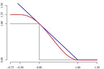
Figure 1.5: Plot of a smooth and bounded function (red) which upper bounds the 0/1 loss and lower bounds the hinge loss.

Lemma 1.13.

Suppose that we sample a training set of size $n$, with $n$ given by the following equation, for parameters $L,B,\epsilon>0$ and $\delta\in\left(0,1\right)$:

$$n=\tilde{O}\left(\left(\frac{L}{\epsilon}\right)\frac{\left(B+\sqrt{\log\frac{1}{\delta}}\right)^{2}}{\epsilon}\right)$$ (1.14)

Then, with probability $1-\delta$ over the i.i.d. training sample $x_{i},y_{i}:i\in\left\{1,\dots,n\right\}$, uniformly for all $w$ satisfying:

$$\left\lVert{w}\right\rVert\leq B,\ \ \hat{\mathcal{L}}_{\mathrm{hinge}}\left(g_{w}\right)\leq L$$ (1.15)

we have that $\mathcal{L}_{\mathrm{0/1}}\left(g_{w}\right)\leq L+\epsilon$.

Proof.

For a smooth loss function, Theorem 1 of Srebro et al. [56] bounds the expected loss in terms of the empirical loss, plus a factor depending on (among other things) the sample size. Neither the 0/1 nor the hinge losses are smooth, so we will define a bounded and smooth loss function which upper bounds the 0/1 loss and lower-bounds the hinge loss. The particular function which we use doesn’t matter, since its smoothness parameter and upper bound will ultimately be absorbed into the big-Oh notation—all that is needed is the existence of such a function. One such is:

$$\psi\left(x\right)=\left\{\begin{array}[]{lcr}\nicefrac{{5}}{{4}}&\cdots&x<-\nicefrac{{1}}{{2}}\\ -x^{2}-x+1&\cdots&-\nicefrac{{1}}{{2}}\leq x<0\\ x^{3}-x^{2}-x+1&\cdots&0\leq x<1\\ 0&\cdots&x\geq 1\end{array}\right.$$

This function, illustrated in Figure 1.5, is $4$-smooth and $\nicefrac{{5}}{{4}}$-bounded. If we define $\mathcal{L}_{\mathrm{smooth}}\left(g_{w}\right)$ and $\hat{\mathcal{L}}_{\mathrm{smooth}}\left(g_{w}\right)$ as the expected and empirical $\psi$-losses, respectively, then the aforementioned theorem gives that, with probability $1-\delta$ uniformly over all $w$ such that $\left\lVert{w}\right\rVert\leq B$:

$$\mathcal{L}_{\mathrm{smooth}}\left(g_{w}\right)\leq\hat{\mathcal{L}}_{\mathrm{smooth}}\left(g_{w}\right)$$

$$+O\left(\frac{B^{2}\log^{3}n}{n}+\frac{\log{\frac{1}{\delta}}}{n}+\sqrt{\hat{\mathcal{L}}_{\mathrm{smooth}}\left(g_{w}\right)}\left(\sqrt{\frac{B^{2}\log^{3}n}{n}}+\sqrt{\frac{\log{\frac{1}{\delta}}}{n}}\right)\right)$$

Because $\psi$ is lower-bounded by the 0/1 loss and upper-bounded by the hinge loss, we may replace $\mathcal{L}_{\mathrm{smooth}}\left(g_{w}\right)$ with $\mathcal{L}_{\mathrm{0/1}}\left(g_{w}\right)$ on the LHS of the above bound, and $\hat{\mathcal{L}}_{\mathrm{smooth}}\left(g_{w}\right)$ with $L$ on the RHS. Setting the big-Oh expression to $\epsilon$ and solving for $n$ then gives the desired result. ∎

While Lemma 1.13 bounds the generalization error of classifiers with empirical hinge loss less than the target value of $L$, the question of how to set $L$ remains unanswered. The following lemma shows that we may take it to be $\mathcal{L}_{\mathrm{hinge}}\left(w^{*}\right)+\epsilon$, where $w^{*}$ minimizes the expected hinge loss:

Lemma 1.16.

Let $u$ be an arbitrary linear classifier, and suppose that we sample a training set of size $n$, with $n$ given by the following equation, for parameters $\epsilon>0$ and $\delta\in\left(0,1\right)$:

$$n=2\left(\frac{\mathcal{L}_{\mathrm{hinge}}\left(g_{u}\right)+\epsilon}{\epsilon}\right)\frac{\left\lVert{u}\right\rVert\log\frac{1}{\delta}}{\epsilon}$$ (1.17)

Then, with probability $1-\delta$ over the i.i.d. training sample $x_{i},y_{i}:i\in\left\{1,\dots,n\right\}$, we have that $\hat{\mathcal{L}}_{\mathrm{hinge}}\left(g_{u}\right)\leq\mathcal{L}_{\mathrm{hinge}}\left(g_{u}\right)+\epsilon$.

Proof.

The hinge loss is upper-bounded by $\left\lVert{u}\right\rVert$ (by assumption, $K(x,x)\leq 1$ with probability $1$, when $x\sim\mathcal{D}$), from which it follows that $\mathrm{Var}_{x,y}\left(\ell\left(y\left\langle{u},{x}\right\rangle\right)\right)\leq\left\lVert{u}\right\rVert\mathcal{L}_{\mathrm{hinge}}\left(g_{u}\right)$. Hence, by Bernstein’s inequality:

$$\mathrm{Pr}\left\{\hat{\mathcal{L}}_{\mathrm{hinge}}\left(g_{u}\right)>\mathcal{L}_{\mathrm{hinge}}\left(g_{u}\right)+\epsilon\right\}\leq \exp\left(-\frac{n}{\left\lVert{u}\right\rVert}\left(\frac{\epsilon^{2}/2}{\mathcal{L}_{\mathrm{hinge}}\left(g_{u}\right)+\epsilon/3}\right)\right)$$

$$\leq \exp\left(-\frac{n}{2\left\lVert{u}\right\rVert}\left(\frac{\epsilon^{2}}{\mathcal{L}_{\mathrm{hinge}}\left(g_{u}\right)+\epsilon}\right)\right)$$

Setting the LHS to $\delta$ and solving for $n$ gives the desired result. ∎

Combining lemmas 1.13 and 1.16 gives us a bound of the desired form, which is given by the following lemma:

lem:svm-introduction:generalization-from-expected-loss

Let $u$ be an arbitrary linear classifier, and suppose that we sample a training set of size $n$, with $n$ given by the following equation, for parameters $B\geq\left\lVert{u}\right\rVert$, $\epsilon>0$ and $\delta\in\left(0,1\right)$:

$$n=\tilde{O}\left(\left(\frac{\mathcal{L}_{\mathrm{hinge}}\left(g_{u}\right)+\epsilon}{\epsilon}\right)\frac{\left(B+\log\frac{1}{\delta}\right)^{2}}{\epsilon}\right)$$ (1.18)

Then, with probability $1-\delta$ over the i.i.d. training sample $x_{i},y_{i}:i\in\left\{1,\dots,n\right\}$, we have that $\hat{\mathcal{L}}_{\mathrm{hinge}}\left(g_{u}\right)\leq\mathcal{L}_{\mathrm{hinge}}\left(g_{u}\right)+\epsilon$ and $\mathcal{L}_{\mathrm{0/1}}\left(g_{w}\right)\leq\hat{\mathcal{L}}_{\mathrm{hinge}}\left(g_{u}\right)+\epsilon$, and in particular that $\mathcal{L}_{\mathrm{0/1}}\left(g_{w}\right)\leq\mathcal{L}_{\mathrm{hinge}}\left(g_{u}\right)+2\epsilon$ uniformly for all $w$ satisfying:

$$\left\lVert{w}\right\rVert\leq B,\ \ \hat{\mathcal{L}}_{\mathrm{hinge}}\left(g_{w}\right)\leq\hat{\mathcal{L}}_{\mathrm{hinge}}\left(g_{u}\right)+\epsilon$$

Lemma 1.16 gives that $\hat{\mathcal{L}}_{\mathrm{hinge}}\left(g_{w}\right)\leq\mathcal{L}_{\mathrm{hinge}}\left(u\right)+2\epsilon$ provided that Equation 1.17 is satisfied. Taking $L=\mathcal{L}_{\mathrm{hinge}}\left(u\right)+2\epsilon$ in Lemma 1.13 gives the desired result, provided that Equation 1.14 is also satisfied. Equation 1.18 is what results from combining these two bounds. The fact that this argument holds with probability $1-2\delta$, while our claim is stated with probability $1-\delta$, is due to the fact that scaling $\delta$ by $1/2$ only changes the bound by a constant.

6.2   Other Proofs

thm:svm-introduction:norm-constrained-runtime

Let $u\in\mathcal{H}$ be an arbitrary reference classifier with $R\geq\left\lVert{u}\right\rVert$. Suppose that we perform $T$ iterations of SGD on the norm-constrained objective, with $w_{t}$ the weight vector after the $t$th iteration. If we define $\bar{w}=\frac{1}{T}\sum_{t=1}^{T}w_{t}$ as the average of these iterates, then there exist values of the training size $n$ and iteration count $T$ such that SGD on the norm-constrained objective with step size $\eta_{t}=R\sqrt{\nicefrac{{2}}{{t}}}$ finds a solution $\bar{w}=\sum_{i=1}^{n}\bar{\alpha}_{i}y_{i}\Phi\left(x_{i}\right)$ satisfying:

$$\mathcal{L}_{\mathrm{0/1}}\left(g_{\bar{w}}\right)\leq\mathcal{L}_{\mathrm{hinge}}\left(g_{u}\right)+\epsilon$$

after performing the following number of kernel evaluations:

$$\mbox{\#K}=\tilde{O}\left(\left(\frac{\mathcal{L}_{\mathrm{hinge}}\left(g_{u}\right)+\epsilon}{\epsilon}\right)\frac{R^{4}}{\epsilon^{3}}\log^{3}\frac{1}{\delta}\right)$$

with the size of the support set of $\bar{w}$ (the number nonzero elements in $\bar{\alpha}$) satisfying:

$$\mbox{\#S}=O\left(\frac{R^{2}}{\epsilon^{2}}\log\frac{1}{\delta}\right)$$

the above statements holding with probability $1-\delta$.

We may bound the online regret of SGD using Zinkevich [66, Theorem 1], which gives the following, if we let $i_{t}$ be the index sampled at the $t$th iteration:

$$\frac{1}{T}\sum_{t=1}^{T}\ell_{\mathrm{hinge}}\left(g_{w_{t}}\left(x_{i_{t}}\right)\right)\leq\frac{1}{T}\sum_{t=1}^{T}\ell_{\mathrm{hinge}}\left(g_{u}\left(x_{i_{t}}\right)\right)+R\sqrt{\frac{1}{2T}}$$

In order to change the above regret bound into a bound on the empirical hinge loss, we use the online-to-batch conversion of Cesa-Bianchi et al. [11, Theorem 1], which gives that with probability $1-\delta$:

$$\hat{\mathcal{L}}_{\mathrm{hinge}}\left(g_{\bar{w}}\right)\leq\hat{\mathcal{L}}_{\mathrm{hinge}}\left(g_{u}\right)+R\sqrt{\frac{1}{2T}}+R\sqrt{\frac{2}{T}\log\frac{1}{\delta}}$$

Which gives that $\bar{w}$ will be $\epsilon$-suboptimal after performing the following number of iterations:’

$$T=O\left(\frac{R^{2}}{\epsilon^{2}}\log\frac{1}{\delta}\right)$$

Because $w$ is projected onto the Euclidean ball of radius $R$ at the end of every iteration, we must have that $\left\lVert{\bar{w}}\right\rVert\leq R$, so we may apply Lemma LABEL:lem:svm-introduction:generalization-from-expected-loss to bound $n$ as (Equation 1.18):

$$n=\tilde{O}\left(\left(\frac{\mathcal{L}_{\mathrm{hinge}}\left(g_{u}\right)+\epsilon}{\epsilon}\right)\frac{\left(R+\log\frac{1}{\delta}\right)^{2}}{\epsilon}\right)$$

The number of kernel evaluations performed over $T$ iterations is $Tn$, and the support size is $T$, which gives the claimed result. thm:svm-introduction:regularized-runtime

Let $u\in\mathcal{H}$ be an arbitrary reference classifier. Suppose that we perform $T$ iterations of Pegasos, with $w_{t}$ the weight vector after the $t$th iteration. If we define $\bar{w}=\frac{1}{T}\sum_{t=1}^{T}w_{t}$ as the average of these iterates, then there exist values of the training size $n$, iteration count $T$ and regularization parameter $\lambda$ such that Pegasos with step size $\eta_{t}=\nicefrac{{1}}{{\lambda t}}$ finds a solution $\bar{w}=\sum_{i=1}^{n}\bar{\alpha}_{i}y_{i}\Phi\left(x_{i}\right)$ satisfying:

$$\mathcal{L}_{\mathrm{0/1}}\left(g_{w}\right)\leq\mathcal{L}_{\mathrm{hinge}}\left(g_{u}\right)+\epsilon$$

after performing the following number of kernel evaluations:

$$\mbox{\#K}=\tilde{O}\left(\min\left(\frac{1}{\epsilon},\left(\frac{\mathcal{L}_{\mathrm{hinge}}\left(g_{u}\right)+\epsilon}{\epsilon}\right)^{2}\right)\frac{\left\lVert{u}\right\rVert^{4}}{\epsilon^{3}}\log^{3}\frac{1}{\delta}\right)$$

with the size of the support set of $w$ (the number nonzero elements in $\bar{\alpha}$) satisfying:

$$\mbox{\#S}=\tilde{O}\left(\frac{\left\lVert{u}\right\rVert^{2}}{\epsilon^{2}}\log\frac{1}{\delta}\right)$$

the above statements holding with probability $1-\delta$.

The analysis of Kakade and Tewari [30, Corollary 7] permits us to bound the suboptimality relative to the reference classifier $u$, with probability $1-\delta$, as:

$$\left(\frac{\lambda}{2}\left\lVert{\bar{w}}\right\rVert^{2}+\hat{\mathcal{L}}_{\mathrm{hinge}}\left(g_{\bar{w}}\right)\right)-\left(\frac{\lambda}{2}\left\lVert{u}\right\rVert^{2}+\hat{\mathcal{L}}_{\mathrm{hinge}}\left(g_{u}\right)\right)\leq\frac{84\log T}{\lambda T}\log\frac{1}{\delta}$$

Solving this equation for $T$ gives that, if one performs the following number of iterations, then the resulting solution will be $\epsilon/2$-suboptimal in the regularized objective, with probability $1-\delta$:

$$T=\tilde{O}\left(\frac{1}{\epsilon}\cdot\frac{r^{2}}{\lambda}\log\frac{1}{\delta}\right)$$

We next follow Shalev-Shwartz and Srebro [51] by decomposing the suboptimality in the empirical hinge loss as:

$$\hat{\mathcal{L}}_{\mathrm{hinge}}\left(g_{\bar{w}}\right)-\hat{\mathcal{L}}_{\mathrm{hinge}}\left(g_{u}\right) =\frac{\epsilon}{2}-\frac{\lambda}{2}\left\lVert{\bar{w}}\right\rVert^{2}+\frac{\lambda}{2}\left\lVert{u}\right\rVert^{2}$$

$$\leq\frac{\epsilon}{2}+\frac{\lambda}{2}\left\lVert{u}\right\rVert^{2}$$

In order to have both terms bounded by $\epsilon/2$, we choose $\lambda=\epsilon/\left\lVert{u}\right\rVert^{2}$, which reduces the RHS of the above to $\epsilon$. Continuing to use this choice of $\lambda$, we next decompose the squared norm of $\bar{w}$ as:

$$\frac{\lambda}{2}\left\lVert{\bar{w}}\right\rVert^{2} =\frac{\epsilon}{2}-\hat{\mathcal{L}}_{\mathrm{hinge}}\left(g_{\bar{w}}\right)+\hat{\mathcal{L}}_{\mathrm{hinge}}\left(g_{u}\right)+\frac{\lambda}{2}\left\lVert{u}\right\rVert^{2}$$

$$\leq\frac{\epsilon}{2}+\hat{\mathcal{L}}_{\mathrm{hinge}}\left(g_{u}\right)+\frac{\lambda}{2}\left\lVert{u}\right\rVert^{2}$$

$$\left\lVert{\bar{w}}\right\rVert^{2} \leq 2\left(\frac{\hat{\mathcal{L}}_{\mathrm{hinge}}\left(g_{u}\right)+\epsilon}{\epsilon}\right)\left\lVert{u}\right\rVert^{2}$$

Hence, we will have that:

$$\left\lVert{\bar{w}}\right\rVert^{2} \leq 2\left(\frac{\hat{\mathcal{L}}_{\mathrm{hinge}}\left(g_{u}\right)+\epsilon}{\epsilon}\right)\left\lVert{u}\right\rVert^{2}$$

$$\hat{\mathcal{L}}_{\mathrm{hinge}}\left(g_{\bar{w}}\right)-\hat{\mathcal{L}}_{\mathrm{hinge}}\left(g_{u}\right) \leq\epsilon$$

with probability $1-\delta$, after performing the following number of iterations:

$$T=\tilde{O}\left(\frac{\left\lVert{u}\right\rVert^{2}}{\epsilon^{2}}\log\frac{1}{\delta}\right)$$ (1.19)

There are two ways in which we will use this bound on $T$ to find bound on the number of kernel evaluations required to achieve some desired error. The easiest is to note that the bound of Equation 1.19 exceeds that of Lemma LABEL:lem:svm-introduction:generalization-from-expected-loss, so that if we take $T=n$, then with high probability, we’ll achieve generalization error $2\epsilon$ after $Tn=T^{2}$ kernel evaluations, in which case:

$$\mbox{\#K}=\tilde{O}\left(\frac{\left\lVert{u}\right\rVert^{4}}{\epsilon^{4}}\log^{2}\frac{1}{\delta}\right)$$

Because we take the number of iterations to be precisely the same as the number of training examples, this is essentially the online stochastic setting.

Alternatively, we may combine our bound on $T$ with Lemma LABEL:lem:svm-introduction:generalization-from-expected-loss. This yields the following bound on the generalization error of Pegasos in the data-laden batch setting.

$$\mbox{\#K}=\tilde{O}\left(\left(\frac{\mathcal{L}_{\mathrm{hinge}}\left(g_{u}\right)+\epsilon}{\epsilon}\right)^{2}\frac{\left\lVert{u}\right\rVert^{4}}{\epsilon^{3}}\log^{3}\frac{1}{\delta}\right)$$

Combining these two bounds on #K gives the claimed result. thm:svm-sbp:perceptron-runtime

Let $u\in\mathcal{H}$ be an arbitrary reference classifier. There exists a value of the training size $n$ such that when the Perceptron algorithm is run for a single “pass” over the dataset, the result is a solution $w=\sum_{i=1}^{n}\alpha_{i}y_{i}\Phi\left(x_{i}\right)$ satisfying:

$$\mathcal{L}_{\mathrm{0/1}}\left(g_{w}\right)\leq\mathcal{L}_{\mathrm{hinge}}\left(g_{u}\right)+\epsilon$$

after performing the following number of kernel evaluations:

$$\mbox{\#K}=\tilde{O}\left(\left(\frac{\mathcal{L}_{\mathrm{hinge}}\left(g_{u}\right)+\epsilon}{\epsilon}\right)^{3}\frac{\left\lVert{u}\right\rVert^{4}}{\epsilon}\frac{1}{\delta}\right)$$

with the size of the support set of $w$ (the number nonzero elements in $\alpha$) satisfying:

$$\mbox{\#S}=O\left(\left(\frac{\mathcal{L}_{\mathrm{hinge}}\left(g_{u}\right)+\epsilon}{\epsilon}\right)^{2}\left\lVert{u}\right\rVert^{2}\frac{1}{\delta}\right)$$

the above statements holding with probability $1-\delta$.

If we run the online Perceptron algorithm for a single pass over the dataset, then Corollary 5 of [49] gives the following mistake bound, for $\mathcal{M}$ being the set of iterations on which a mistake is made:

$$\left\lvert{\mathcal{M}}\right\rvert\leq\sum_{i\in\mathcal{M}}\ell\left(y_{i}\left\langle{u},{\Phi\left(x_{i}\right)}\right\rangle\right)$$ (1.20)

$$+\left\lVert{u}\right\rVert\sqrt{\sum_{i\in\mathcal{M}}\ell\left(y_{i}\left\langle{u},{\Phi\left(x_{i}\right)}\right\rangle\right)}+\left\lVert{u}\right\rVert^{2}$$

$$\sum_{i=1}^{n}\ell_{0/1}\left(y_{i}\left\langle{w_{i}},{\Phi\left(x_{i}\right)}\right\rangle\right)\leq\sum_{i=1}^{n}\ell\left(y_{i}\left\langle{u},{\Phi\left(x_{i}\right)}\right\rangle\right)+$$

$$+\left\lVert{u}\right\rVert\sqrt{\sum_{i=1}^{n}\ell\left(y_{i}\left\langle{u},{\Phi\left(x_{i}\right)}\right\rangle\right)}+r^{2}\left\lVert{u}\right\rVert^{2}$$

Here, $\ell$ is the hinge loss and $\ell_{0/1}$ is the 0/1 loss. Dividing through by $n$:

$$\frac{1}{n}\sum_{i=1}^{n}\ell_{0/1}\left(y_{i}\left\langle{w_{i}},{\Phi\left(x_{i}\right)}\right\rangle\right)\leq\frac{1}{n}\sum_{i=1}^{n}\ell\left(y_{i}\left\langle{u},{\Phi\left(x_{i}\right)}\right\rangle\right)$$

$$+\frac{r\left\lVert{u}\right\rVert}{\sqrt{n}}\sqrt{\frac{1}{n}\sum_{i=1}^{n}\ell\left(y_{i}\left\langle{u},{\Phi\left(x_{i}\right)}\right\rangle\right)}+\frac{\left\lVert{u}\right\rVert^{2}}{n}$$

If we suppose that the $x_{i},y_{i}$s are i.i.d., and that $w\sim\mbox{Unif}\left(w_{1},\dots,w_{n}\right)$ (this is a “sampling” online-to-batch conversion), then:

$$\mathbb{E}\left[\mathcal{L}_{\mathrm{0/1}}\left(g_{w}\right)\right]\leq\mathcal{L}_{\mathrm{hinge}}\left(g_{u}\right)+\frac{r\left\lVert{u}\right\rVert}{\sqrt{n}}\sqrt{\mathcal{L}_{\mathrm{hinge}}\left(g_{u}\right)}+\frac{\left\lVert{u}\right\rVert^{2}}{n}$$

Hence, the following will be satisfied:

$$\mathbb{E}\left[\mathcal{L}_{\mathrm{0/1}}\left(g_{w}\right)\right]\leq\mathcal{L}_{\mathrm{hinge}}\left(g_{u}\right)+\epsilon$$ (1.21)

when:

$$n\leq O\left(\left(\frac{\mathcal{L}_{\mathrm{hinge}}\left(g_{u}\right)+\epsilon}{\epsilon}\right)\frac{\left\lVert{u}\right\rVert^{2}}{\epsilon}\right)$$

The expectation is taken over the random sampling of $w$. The number of kernel evaluations performed by the $i$th iteration of the Perceptron will be equal to the number of mistakes made before iteration $i$. This quantity is upper bounded by the total number of mistakes made over $n$ iterations, which is given by the mistake bound of equation 1.20:

$$\left\lvert{\mathcal{M}}\right\rvert\leq n\mathcal{L}_{\mathrm{hinge}}\left(g_{u}\right)+r\left\lVert{u}\right\rVert\sqrt{n\mathcal{L}_{\mathrm{hinge}}\left(g_{u}\right)}+\left\lVert{u}\right\rVert^{2}$$

$$\leq O\left(\left(\frac{1}{\epsilon}\left(\frac{\mathcal{L}_{\mathrm{hinge}}\left(g_{u}\right)+\epsilon}{\epsilon}\right)\mathcal{L}_{\mathrm{hinge}}\left(g_{u}\right)\right.\right.$$

$$\left.\left.+\sqrt{\frac{1}{\epsilon}\left(\frac{\mathcal{L}_{\mathrm{hinge}}\left(g_{u}\right)+\epsilon}{\epsilon}\right)\mathcal{L}_{\mathrm{hinge}}\left(g_{u}\right)}+1\right)\left\lVert{u}\right\rVert^{2}\right)$$

$$\leq O\left(\left(\left(\frac{\mathcal{L}_{\mathrm{hinge}}\left(g_{u}\right)+\epsilon}{\epsilon}\right)^{2}-\left(\frac{\mathcal{L}_{\mathrm{hinge}}\left(g_{u}\right)+\epsilon}{\epsilon}\right)\right.\right.$$

$$\left.\left.+\sqrt{\left(\frac{\mathcal{L}_{\mathrm{hinge}}\left(g_{u}\right)+\epsilon}{\epsilon}\right)^{2}-\left(\frac{\mathcal{L}_{\mathrm{hinge}}\left(g_{u}\right)+\epsilon}{\epsilon}\right)}+1\right)r^{2}\left\lVert{u}\right\rVert^{2}\right)$$

$$\leq O\left(\left(\frac{\mathcal{L}_{\mathrm{hinge}}\left(g_{u}\right)+\epsilon}{\epsilon}\right)^{2}\left\lVert{u}\right\rVert^{2}\right)$$

The number of mistakes $\left\lvert{\mathcal{M}}\right\rvert$ is necessarily equal to the size of the support set of the resulting classifier. Substituting this bound into the number of iterations:

$$\mbox{\#K}= n\left\lvert{\mathcal{M}}\right\rvert$$

$$\leq O\left(\left(\frac{\mathcal{L}_{\mathrm{hinge}}\left(g_{u}\right)+\epsilon}{\epsilon}\right)^{3}\frac{\left\lVert{u}\right\rVert^{4}}{\epsilon}\right)$$

This holds in expectation, but we can turn this into a high-probability result using Markov’s inequality, resulting in in a $\delta$-dependence of $\frac{1}{\delta}$. thm:svm-sbp:projection-runtime

Let $u\in\mathcal{H}$ be an arbitrary reference classifier which is written in terms of the training data as $u=\sum_{i=1}^{n}\alpha_{i}y_{i}\Phi\left(x_{i}\right)$. Suppose that we perform the approximation procedure of Rahimi and Recht [47] to yield a $2D$-dimensional linear approximation to the original kernelized classification problem, and define $\tilde{u}=\sum_{i=1}^{n}\alpha_{i}y_{i}\tilde{\Phi}\left(x_{i}\right)$. There exists a value of the approximate linear SVM dimension $D$:

$$D=\tilde{O}\left(\frac{d\left\lVert{\alpha}\right\rVert_{1}^{2}}{\epsilon^{2}}\log\frac{1}{\delta}\right)$$

as well as a training size $n$, such that, if the resulting number of features satisfies:

$$nD=\tilde{O}\left(\left(\frac{\mathcal{L}_{\mathrm{hinge}}\left(g_{u}\right)+\epsilon}{\epsilon}\right)\frac{d\left\lVert{\alpha}\right\rVert_{1}^{4}}{\epsilon^{3}}\log^{3}\frac{1}{\delta}\right)$$

Then for any $w\in\mathbb{R}^{2D}$ solving the resulting approximate linear problem such that:

$$\left\lVert{w}\right\rVert\leq\left(1+\sqrt{\frac{\epsilon}{\left\lVert{\alpha}\right\rVert_{1}}}\right)\left\lVert{\alpha}\right\rVert_{1},\ \ \hat{\mathcal{L}}_{\mathrm{hinge}}\left(g_{w}\right)\leq\hat{\mathcal{L}}_{\mathrm{hinge}}\left(g_{\tilde{u}}\right)+\epsilon$$

we will have that $\mathcal{L}_{\mathrm{0/1}}\left(g_{w}\right)\leq\mathcal{L}_{\mathrm{hinge}}\left(g_{u}\right)+3\epsilon$, with this result holding with probability $1-\delta$. Notice that we have abused notation slightly here—losses of $g_{u}$ are for the original kernel problem, while losses of $g_{w}$ and $g_{\tilde{u}}$ are of the approximate linear SVM problem.

Hoeffding’s inequality yields [47, Claim 1] that, in order to ensure that $\left\lvert{K(x,x^{\prime})-\left\langle{\tilde{\Phi}(x)},{\tilde{\Phi}(x^{\prime})}\right\rangle}\right\rvert<\tilde{\epsilon}$ uniformly for all $x,x^{\prime}\in\mathbb{R}^{d}$ with probability $1-\delta$, the following number of random Fourier features are required:

$$D=O\left(\frac{d}{\tilde{\epsilon}^{2}}\log\left(\frac{1}{\delta\tilde{\epsilon}^{2}}\right)\right)$$

Here, the proportionality constant hidden inside the big-Oh notation varies depending on the particular kernel in which we are interested, and a uniform bound on the $2$-norm of $x\in\mathcal{X}$. This result is not immediately applicable, because the quantities which we need in order to derive a generalization bound are the norm of the predictor, and the error in each classification (rather than the error in each kernel evaluation). Applying the above bound yields that:

$$\left\lvert{\ell_{\mathrm{hinge}}\left(y\left\langle{u},{\Phi\left(x\right)}\right\rangle\right)-\ell_{\mathrm{hinge}}\left(y\left\langle{\tilde{u}},{\tilde{\Phi}\left(x\right)}\right\rangle\right)}\right\rvert$$

$$\leq\left\lvert{\left\langle{u},{\Phi\left(x\right)}\right\rangle-\left\langle{\tilde{u}},{\tilde{\Phi}\left(x\right)}\right\rangle}\right\rvert$$

$$=\left\lvert{\sum_{i=1}^{n}\alpha_{i}y_{i}\left(K\left(x_{i},x\right)-\left\langle{\tilde{\Phi}\left(x_{i}\right)},{\tilde{\Phi}\left(x\right)}\right\rangle\right)}\right\rvert$$

$$\leq\tilde{\epsilon}\left\lVert{\alpha}\right\rVert_{1}$$

and:

$$\left\lvert{\left\lVert{u}\right\rVert^{2}-\left\lVert{\tilde{u}}\right\rVert^{2}}\right\rvert= \left\lvert{\sum_{i=1}^{n}\sum_{j=1}^{n}\alpha_{i}\alpha_{j}y_{i}y_{j}\left(K\left(x_{i},x_{j}\right)-\left\langle{\tilde{\Phi}\left(x_{i}\right)},{\tilde{\Phi}\left(x_{j}\right)}\right\rangle\right)}\right\rvert$$

$$\leq \tilde{\epsilon}\left\lVert{\alpha}\right\rVert_{1}^{2}$$

Observe that, because $K(x,x)\leq 1$ by assumption, $\left\lVert{u}\right\rVert_{2}\leq\left\lVert{u}\right\rVert_{1}$. Hence, if we take $B=\left(1+\sqrt{\tilde{\epsilon}}\right)\left\lVert{\alpha}\right\rVert_{1}$ so that $B^{2}\geq\left\lVert{u}\right\rVert^{2}+\tilde{\epsilon}\left\lVert{\alpha}\right\rVert_{1}^{2}$ in Lemma LABEL:lem:svm-introduction:generalization-from-expected-loss, we will have that all $\tilde{w}\in\mathbb{R}^{2D}$ satisfying $\left\lVert{w}\right\rVert\leq B$ and $\hat{\mathcal{L}}_{\mathrm{hinge}}\left(g_{w}\right)\leq\hat{\mathcal{L}}_{\mathrm{hinge}}\left(g_{u}\right)+\epsilon$ generalize as $\mathcal{L}_{\mathrm{0/1}}\left(g_{w}\right)\leq\mathcal{L}_{\mathrm{hinge}}\left(g_{\tilde{u}}\right)+2\epsilon$, as long as:

$$n=\tilde{O}\left(\left(\frac{\mathcal{L}_{\mathrm{hinge}}\left(g_{u}\right)+\epsilon}{\epsilon}\right)\frac{\left(\left(1+\sqrt{\tilde{\epsilon}}\right)\left\lVert{\alpha}\right\rVert_{1}+\log\frac{1}{\delta}\right)^{2}}{\epsilon}\right)$$

Taking $\tilde{\epsilon}=\nicefrac{{\epsilon}}{{\left\lVert{\alpha}\right\rVert_{1}}}$, multiplying the bounds on $n$ and $D$, and observing that $\mathcal{L}_{\mathrm{hinge}}\left(g_{\tilde{u}}\right)\leq\mathcal{L}_{\mathrm{hinge}}\left(g_{u}\right)+\epsilon$ completes the proof.

The Kernelized Stochastic Batch Perceptron

7   Overview

In this chapter, we will present a novel algorithm for training kernel Support Vector Machines (SVMs), and establish learning runtime guarantees which are better then those for any other known kernelized SVM optimization approach. We also show experimentally that our method works well in practice compared to existing SVM training methods. The content of this chapter was originally presented in the 29th International Conference on Machine Learning (ICML 2012) [18].

Our method is a stochastic gradient method on a non-standard scalarization of the bi-criterion SVM objective of Problem 1.1 in Chapter 1. In particular, we use the “slack constrained” scalarized optimization problem introduced by Hazan et al. [25], where we seek to maximize the classification margin, subject to a constraint on the total amount of “slack”, i.e. sum of the violations of this margin. Our approach is based on an efficient method for computing unbiased gradient estimates on the objective. Our algorithm can be seen as a generalization of the “Batch Perceptron” to the non-separable case (i.e. when errors are allowed), made possible by introducing stochasticity, and we therefore refer to it as the “Stochastic Batch Perceptron” (SBP).

The SBP is fundamentally different from other stochastic gradient approaches to the problem of training SVMs (such as SGD on the norm-constrained and regularized objectives of Section 2 in Chapter 1, see Section 4 for details), in that calculating each stochastic gradient estimate still requires considering the entire data set. In this regard, despite its stochasticity, the SBP is very much a “batch” rather than “online” algorithm. For a linear SVM, each iteration would require runtime linear in the training set size, resulting in an unacceptable overall runtime. However, in the kernel setting, essentially all known approaches already require linear runtime per iteration. A more careful analysis reveals the benefits of the SBP over previous kernel SVM optimization algorithms.

As was done in Chapter 1, we follow Bottou and Bousquet [5], Shalev-Shwartz and Srebro [51] and compare the runtimes required to ensure a generalization error of $L^{*}+\epsilon$, assuming the existence of some unknown predictor $u$ with norm $\left\lVert{u}\right\rVert$ and expected hinge loss $L^{*}$. We derive an “optimistic” bound, as described in Section 3 of Chapter 1, for which the main advantage of the SBP over competing algorithms is in the “easy” regime: when $\epsilon=\Omega(L^{*})$ (i.e. we seek a constant factor approximation to the best achievable error, such as if we desire an error of $1.01L^{*}$). In such a case, the overall SBP runtime is $\left\lVert{u}\right\rVert^{4}/\epsilon$, compared with $\left\lVert{u}\right\rVert^{4}/\epsilon^{3}$ for Pegasos and $\left\lVert{u}\right\rVert^{4}/\epsilon^{2}$ for the best known dual decomposition approach.

8   Setup and Formulations

In Section 2 of Chapter 1, the bi-criterion SVM objective was presented, along with several of the equivalent scalarizations of this objective which are optimized by various popular algorithms. The SBP relies on none of these, but rather on the “slack constrained” scalarization [25], for which we maximize the “margin” subject to a constraint of $\nu$ on the total allowed “slack”, corresponding to the average error. That is, we aim at maximizing the margin by which all points are correctly classified (i.e. the minimal distance between a point and the separating hyperplane), after allowing predictions to be corrected by a total amount specified by the slack constraint:

$$\max_{w\in\mathbb{R}^{d}}\max_{\xi\in\mathbb{R}^{n}}\min_{i\in\left\{1,\dots,n\right\}} \left(y_{i}\left\langle{w},{\Phi\left(x_{i}\right)}\right\rangle+\xi_{i}\right)$$ (2.1)

subject to: $$\left\lVert{w}\right\rVert\leq 1,\leavevmode\nobreak\ \xi\succeq 0,\leavevmode\nobreak\ \mathbf{1}^{T}\xi\leq n\nu$$

This scalarization is equivalent to the original bi-criterion objective in that varying $\nu$ explores different Pareto optimal solutions of Problem 1.1. This is captured by the following Lemma, which also quantifies how suboptimal solutions of the slack-constrained objective correspond to Pareto suboptimal points:

Lemma 2.2.

For any $u\neq 0$, consider Problem 2.1 with $\nu=\hat{\mathcal{L}}_{\mathrm{hinge}}\left(g_{u}\right)/\left\lVert{u}\right\rVert$. Let $\bar{w}$ be an $\bar{\epsilon}$-suboptimal solution to this problem with objective value $\gamma$, and consider the rescaled solution $w=\bar{w}/\gamma$. Then:

$$\left\lVert{w}\right\rVert\leq \frac{1}{1-\bar{\epsilon}\left\lVert{u}\right\rVert}\left\lVert{u}\right\rVert\leavevmode\nobreak\ \leavevmode\nobreak\ ,\leavevmode\nobreak\ \leavevmode\nobreak\ \hat{\mathcal{L}}_{\mathrm{hinge}}\left(g_{w}\right)\leq\frac{1}{1-\bar{\epsilon}\left\lVert{u}\right\rVert}\hat{\mathcal{L}}_{\mathrm{hinge}}\left(g_{u}\right)$$

Proof.

This is Lemma 2.1 of Hazan et al. [25]. ∎

9   The Stochastic Batch Perceptron

In this section, we will develop the Stochastic Batch Perceptron. We consider Problem 2.1 as optimization of the variable $w$ with a single constraint $\left\lVert{w}\right\rVert\leq 1$, with the objective being to maximize:

$$f\left(w\right)\leavevmode\nobreak\ =\max_{\xi\succeq 0,\mathbf{1}^{T}\xi\leq n\nu}\leavevmode\nobreak\ \leavevmode\nobreak\ \min_{p\in\Delta^{n}}\leavevmode\nobreak\ \leavevmode\nobreak\ \sum_{i=1}^{n}p_{i}\left(y_{i}\left\langle{w},{\Phi\left(x_{i}\right)}\right\rangle+\xi_{i}\right)$$ (2.3)

Notice that we replaced the minimization over training indices $i$ in Problem 2.1 with an equivalent minimization over the probability simplex, $\Delta^{n}=\{p\succeq 0:\mathbf{1}^{T}p=1\}$, and that we consider $p$ and $\xi$ to be a part of the objective, rather than optimization variables. The objective $f(w)$ is a concave function of $w$, and we are maximizing it over a convex constraint $\left\lVert{w}\right\rVert\leq 1$, and so this is a convex optimization problem in $w$.

Our approach will be to perform a stochastic gradient update on $w$ at each iteration: take a step in the direction specified by an unbiased estimator of a (super)gradient of $f(w)$, and project back to $\left\lVert{w}\right\rVert\leq 1$. To this end, we will need to identify the (super)gradients of $f(w)$ and understand how to efficiently calculate unbiased estimates of them.

9.1   Warmup: The Separable Case

As a warmup, we first consider the separable case, where $\nu=0$ and no errors are allowed. The objective is then:

$$f(w)=\min_{i}y_{i}\left\langle{w},{\Phi\left(x_{i}\right)}\right\rangle,$$ (2.4)

This is simply the “margin” by which all points are correctly classified, i.e. $\gamma$ s.t. $\forall_{i}\leavevmode\nobreak\ y_{i}\left\langle{w},{\Phi(x_{i})}\right\rangle\geq\gamma$. We seek a linear predictor $w$ with the largest possible margin. It is easy to see that (super)gradients with respect to $w$ are given by $y_{i}\Phi(x_{i})$ for any index $i$ attaining the minimum in Equation 2.4, i.e. by the “most poorly classified” point(s). A gradient ascent approach would then be to iteratively find such a point, update $w\leftarrow w+\eta y_{i}\Phi(x_{i})$, and project back to $\left\lVert{w}\right\rVert\leq 1$. This is akin to a “batch Perceptron” update, which at each iteration searches for a violating point and adds it to the predictor.

In the separable case, we could actually use exact supergradients of the objective. As we shall see, it is computationally beneficial in the non-separable case to base our steps on unbiased gradient estimates. We therefore refer to our method as the “Stochastic Batch Perceptron” (SBP), and view it as a generalization of the batch Perceptron which uses stochasticity and is applicable in the non-separable setting. In the same way that the “batch Perceptron” can be used to maximize the margin in the separable case, the SBP can be used to obtain any SVM solution along the Pareto front of the bi-criterion Problem 1.1.

9.2   Supergradients of $f(w)$

Figure 2.1: Illustration of how one finds $\xi^{*}$ and $p^{*}$. The upper curve represents the values of the responses $c_{i}$, listed in order of increasing magnitude. The lower curve illustrates a minimax optimal probability distribution $p^{*}$.

Recall that, in Chapter 1, we defined the vector of “responses” $c\in\mathbb{R}^{n}$ to be, for a fixed $w$:

$$c_{i}=y_{i}\left\langle{w},{\Phi\left(x_{i}\right)}\right\rangle$$ (2.5)

The objective of the max-min optimization problem in the definition of $f(w)$ can be written as $p^{T}(c+\xi)$. Supergradients of $f(w)$ at $w$ can be characterized explicitly in terms of minimax-optimal pairs $p^{*}$ and $\xi^{*}$ such that $p^{*}=\operatorname{argmin}_{p\in\Delta^{n}}p^{t}(c+\xi^{*})$ and $\xi^{*}=\operatorname{argmax}_{\xi\succeq 0,\mathbf{1}^{T}\xi\leq n\nu}(p^{*})^{T}(c+\xi)$.

lem:svm-sbp:slack-constrained-supergradient

For any $w$, let $p^{*},\xi^{*}$ be minimax optimal for Equation 2.3. Then $\sum_{i=1}^{n}p^{*}_{i}y_{i}\Phi\left(x_{i}\right)$ is a supergradient of $f(w)$ at $w$.

By the definition of $f$, for any $v\in\mathbb{R}^{d}$:

$$f\left(w+v\right)=\max_{\xi\succeq 0,\mathbf{1}^{T}\xi\leq n\nu}\min_{p\in\Delta^{n}}\sum_{i=1}^{n}p_{i}\left(y_{i}\left\langle{w+v},{\Phi\left(x_{i}\right)}\right\rangle+\xi_{i}\right)$$

Substituting the particular value $p^{*}$ for $p$ can only increase the RHS, so:

$$f\left(w+v\right)\leq \max_{\xi\succeq 0,\mathbf{1}^{T}\xi\leq n\nu}\sum_{i=1}^{n}p^{*}_{i}\left(y_{i}\left\langle{w+v},{\Phi\left(x_{i}\right)}\right\rangle+\xi_{i}\right)$$

$$\leq \max_{\xi\succeq 0,\mathbf{1}^{T}\xi\leq n\nu}\sum_{i=1}^{n}p^{*}_{i}\left(y_{i}\left\langle{w},{\Phi\left(x_{i}\right)}\right\rangle+\xi_{i}\right)+\sum_{i=1}^{n}p^{*}_{i}y_{i}\left\langle{v},{\Phi\left(x_{i}\right)}\right\rangle$$

Because $p^{*}$ is minimax-optimal at $w$:

$$f\left(w+v\right)\leq f\left(w\right)+\sum_{i=1}^{n}p^{*}_{i}y_{i}\left\langle{v},{\Phi\left(x_{i}\right)}\right\rangle$$

$$\leq f\left(w\right)+\left\langle{v},{\sum_{i=1}^{n}p^{*}_{i}y_{i}\Phi\left(x_{i}\right)}\right\rangle$$

So $\sum_{i=1}^{n}p^{*}_{i}y_{i}\Phi\left(x_{i}\right)$ is a supergradient of $f$.

This suggests a simple method for obtaining unbiased estimates of supergradients of $f(w)$: sample a training index $i$ with probability $p^{*}_{i}$, and take the stochastic supergradient to be $y_{i}\Phi\left(x_{i}\right)$. The only remaining question is how one finds a minimax optimal $p^{*}$.

For any $\xi$, a solution of $\min_{p\in\Delta^{n}}p^{T}(x+\xi)$ must put all of the probability mass on those indices $i$ for which $c_{i}+\xi_{i}$ is minimized. Hence, an optimal $\xi^{*}$ will maximize the minimal value of $c_{i}+\xi^{*}_{i}$. This is illustrated in Figure 2.1. The intuition is that the total mass $n\nu$ available to $\xi$ is distributed among the indices as if this volume of water were poured into a basin with height $c_{i}$. The result is that the indices $i$ with the lowest responses have columns of water above them such that the common surface level of the water is $\gamma$.

Once the “water level” $\gamma$ has been determined, we may find the probability distribution $p$. Note first that, in order for $p$ to be optimal at $\xi^{*}$, it must be supported on a subset of those indices $i$ for which $c_{i}+\xi^{*}_{i}=\gamma$, since any such choice results in $p^{T}\left(c+\xi^{*}\right)=\gamma$, while any choice supported on another set of indices must have $p^{T}\left(c+\xi^{*}\right)>\gamma$.

However, merely being supported on this set is insufficient for minimax optimality. If $i$ and $j$ are two indices with $\xi^{*}_{i},\xi^{*}_{j}>0$, and $p_{i}>p_{j}$, then $p^{T}\left(x+\xi^{*}\right)$ could be made larger by increasing $\xi^{*}_{i}$ and decreasing $\xi^{*}_{j}$ by the same amount. Hence, we must have that $p^{*}$ takes on the constant value $q$ on all indices $i$ for which $\xi^{*}_{i}>0$. What about if $c_{i}=\gamma$ (and therefore $\xi^{*}_{i}=0$)? For such indices, $\xi^{*}_{i}$ cannot be decreased any further, due to the nonnegativity constraint on $\xi$, so we may have that $p_{i}<q$. If $p_{i}>q$, however, then a similar argument to the above shows that $p$ is not minimax optimal.

The final characterization of minimax optimal probability distributions is that $p^{*}_{i}\leq q$ for all indices $i$ such that $c_{i}=\gamma$, and that $p^{*}_{i}=q$ if $c_{i}<\gamma 0$. This is illustrated in the lower portion of Figure 2.1. In particular, the uniform distribution over all indices such that $c_{i}<\gamma$ is minimax optimal.

$\mbox{{find\_gamma}}\left(C:\mathbb{R}^{n},n\nu:\mathbb{R}\right)$
1	$low:=1$; $up:=n$;
2	$low\_max:=-\infty$; $low\_sum:=0$;
3	$\mbox{{while }}low<up$
4		$mid:=\mbox{{partition}}(C\left[low:up\right])$;
5		$mid\_max:=\max\left(low\_max,C\left[low:\left(mid-1\right)\right]\right)$;
6		$mid\_sum:=low\_sum+\sum C\left[low:\left(mid-1\right)\right]$;
7		$\mbox{{if }}mid\_max\cdot\left(mid-1\right)-mid\_sum\geq n\nu\mbox{{ then}}$
8			$up:=mid-1$;
9		$else$
10			$low:=mid$; $low\_max:=mid\_max$; $low\_sum:=mid\_sum$;
11	$\mbox{{return }}\left(n\nu-low\_max\cdot\left(low-1\right)+low\_sum\right)/\left(low-1\right)+low\_max$;

Algorithm 2.2 Divide-and-conquer algorithm for finding the “water level” $\gamma$ from an array of responses $C$ and total volume $n\nu$. The partition function chooses a pivot value from the array it receives as an argument (the median would be ideal), places all values less than the pivot at the start of the array, all values greater at the end, and returns the index of the pivot in the resulting array.

It is straightforward to find the water level $\gamma$ in linear time once the responses $c_{i}$ are sorted (as in Figure 2.1), i.e. with a total runtime of $O(n\log n)$ due to sorting. It is also possible to find the water level $\gamma$ in linear time, without sorting the responses, using a divide-and-conquer algorithm (Algorithm 2.2). This algorithm works by subdividing the set of responses into those less than, equal to and greater than a pivot value (if one uses the median, which can be found in linear time using e.g. the median-of-medians algorithm [4], then the overall will be linear in $n$). Then, it calculates the size, minimum and sum of each of these subsets, from which the total volume of the water required to cover the subsets can be easily calculated. It then recurses into the subset containing the point at which a volume of $n\nu$ just suffices to cover the responses, and continues until $\gamma$ is found.

9.3   Putting it Together

$\mbox{{optimize}}\left(n:\mathbb{N},d:\mathbb{N},x_{1},\dots,x_{n}:\mathbb{R}^{d},y_{1},\dots,y_{n}:\left\{\pm 1\right\},T:\mathbb{N},\nu:\mathbb{R}_{+},K:\mathbb{R}^{d}\times\mathbb{R}^{d}\rightarrow\mathbb{R}_{+}\right)$
1	$\eta_{0}:=1/\sqrt{\max_{i}K\left(x_{i},x_{i}\right)}$;
2	$\alpha^{(0)}:=0^{n}$; $c^{(0)}:=0^{n}$; $r_{0}:=0$;
3	$\mbox{{for }}t:=1\mbox{{ to }}T$
4		$\eta_{t}:=\eta_{0}/\sqrt{t}$;
5		$\gamma:=\mbox{{find\_gamma}}\left(c^{(t-1)},n\nu\right)$;
6		$\mbox{{sample }}i\sim\mbox{{uniform}}\left\{j:c^{(t-1)}_{j}<\gamma\right\}$;
7		$\alpha^{(t)}:=\alpha^{(t-1)}+\eta_{t}e_{i}$;
8		$r_{t}^{2}:=r_{t-1}^{2}+2\eta_{t}c^{(t-1)}_{i}+\eta_{t}^{2}K\left(x_{i},x_{i}\right)$;
9		$\mbox{{for }}j=1\mbox{{ to }}n$
10			$c^{(t)}_{j}:=c^{(t-1)}_{j}+\eta_{t}y_{i}y_{j}K\left(x_{i},x_{j}\right)$;
11		$\mbox{{if }}\left(r_{t}>1\right)\mbox{{ then}}$
12			$\alpha^{(t)}:=\left(1/r_{t}\right)\alpha^{(t)}$; $c^{(t)}:=\left(1/r_{t}\right)c^{(t)}$; $r_{t}:=1$;
13	$\bar{\alpha}:=\frac{1}{T}\sum_{t=1}^{T}\alpha^{(t)}$; $\bar{c}:=\frac{1}{T}\sum_{t=1}^{T}c^{(t)}$; $\gamma:=\mbox{{find\_gamma}}\left(\bar{c},n\nu\right)$;
14	$\mbox{{return }}\bar{\alpha}/\gamma$;

Algorithm 2.3 Stochastic gradient ascent algorithm for optimizing the kernelized version of Problem 2.1. Here, $e_{i}$ is the $i$th standard unit basis vector. The find_gamma subroutine finds the “water level” $\gamma$ from the vector of responses $c$ and total volume $n\nu$.

We are now ready to summarize the SBP algorithm. Starting from $w^{(0)}=0$ (so both $\alpha^{(0)}$ and all responses are zero), each iteration proceeds as follows:

1. Find $p^{*}$ by finding the “water level” $\gamma$ from the responses (Section 9.2), and taking $p^{*}$ to be uniform on those indices for which $c_{i}\leq\gamma$.

2. Sample $j\sim p^{*}$.

3. Update $w^{(t+1)}\leftarrow\mathcal{P}\left(w^{(t)}+\eta_{t}y_{j}\Phi\left(x_{j}\right)\right)$, where $\mathcal{P}$ projects onto the unit ball and $\eta_{t}=\frac{1}{\sqrt{t}}$. This is done by first increasing $\alpha\leftarrow\alpha+\eta_{t}$, updating the responses $c$ accordingly, and projecting onto the set $\left\lVert{w}\right\rVert\leq 1$.

Detailed pseudo-code may be found in Algorithm 2.3—observe that it is an instance of the traditional SVM optimization outline of Section 4 of Chapter 1 (compare to Algorithm 1.4). Updating the responses requires $O(n)$ kernel evaluations (the most computationally expensive part) and all other operations require $O(n)$ scalar arithmetic operations.

Since at each iteration we are just updating using an unbiased estimator of a supergradient, we can rely on the standard analysis of stochastic gradient descent to bound the suboptimality after $T$ iterations:

lem:svm-sbp:zinkevich-batch

For any $T,\delta>0$, after $T$ iterations of the Stochastic Batch Perceptron, with probability at least $1-\delta$, the average iterate $\bar{w}=\frac{1}{T}\sum_{t=1}^{T}w^{(t)}$ (corresponding to $\bar{\alpha}=\frac{1}{T}\sum_{t=1}^{T}\alpha^{(t)}$), satisfies: $f\left(\bar{w}\right)\geq\sup_{\left\lVert{w}\right\rVert\leq 1}f\left(w\right)-O\left(\sqrt{\frac{1}{T}\log\frac{1}{\delta}}\right).$

Define $h=-\frac{1}{r}f$, where $f$ is as in Equation 2.3. Then the stated update rules constitute an instance of Zinkevich’s algorithm, in which steps are taken in the direction of stochastic subgradients $g^{(t)}$ of $h$ at $w^{(t)}=\sum_{i=1}^{n}\alpha_{i}y_{i}\Phi\left(x_{i}\right)$.

The claimed result follows directly from Zinkevich [66, Theorem 1] combined with an online-to-batch conversion analysis in the style of Cesa-Bianchi et al. [11, Lemma 1].

Since each iteration is dominated by $n$ kernel evaluations, and thus takes linear time (we take a kernel evaluation to require $O(1)$ time), the overall runtime to achieve $\epsilon$ suboptimality for Problem 2.1 is $O(n/\epsilon^{2})$.

9.4   Learning Runtime

The previous section has given us the runtime for obtaining a certain suboptimality of Problem 2.1. However, since the suboptimality in this objective is not directly comparable to the suboptimality of other scalarizations, e.g. Problem 1.3, we follow Bottou and Bousquet [5], Shalev-Shwartz and Srebro [51], and analyze the runtime required to achieve a desired generalization performance, instead of that to achieve a certain optimization accuracy on the empirical optimization problem.

Recall that our true learning objective is to find a predictor with low generalization error $\mathcal{L}_{\mathrm{0/1}}\left(g_{w}\right)=\mathrm{Pr}_{(x,y)}\left\{y\left\langle{w},{\Phi(x)}\right\rangle\leq 0\right\}$ with respect to some unknown distribution over $x,y$ based on a training set drawn i.i.d. from this distribution. We assume that there exists some (unknown) predictor $u$ that has norm $\left\lVert{u}\right\rVert$ and low expected hinge loss $L^{*}=\mathcal{L}_{\mathrm{hinge}}\left(g_{u}\right)=\mathbb{E}\left[\ell(y\left\langle{u},{\Phi(x)}\right\rangle)\right]$ (otherwise, there is no point in training a SVM), and analyze the runtime to find a predictor $w$ with generalization error $\mathcal{L}_{\mathrm{0/1}}\left(g_{w}\right)\leq L^{*}+\epsilon$.

In order to understand the SBP runtime, we will follow Hazan et al. [25] by optimizing the empirical SVM bi-criterion Problem 1.1 such that:

$$\left\lVert{w}\right\rVert \leq 2\left\lVert{u}\right\rVert\leavevmode\nobreak\ \leavevmode\nobreak\ ;\leavevmode\nobreak\ \leavevmode\nobreak\ \hat{\mathcal{L}}_{\mathrm{hinge}}\left(g_{w}\right)-\hat{\mathcal{L}}_{\mathrm{hinge}}\left(g_{u}\right)\leq\epsilon/2$$ (2.6)

which suffices to ensure $\mathcal{L}_{\mathrm{0/1}}\left(g_{w}\right)\leq L^{*}+\epsilon$ with high probability. Referring to Lemma 2.2, Equation 2.6 will be satisfied for $\bar{w}/\gamma$ as long as $\bar{w}$ optimizes the objective of Problem 2.1 to within:

$$\bar{\epsilon}=\frac{\epsilon/2}{\left\lVert{u}\right\rVert(\hat{\mathcal{L}}_{\mathrm{hinge}}\left(g_{u}\right)+\epsilon/2)}\geq\Omega\left(\frac{\epsilon}{\left\lVert{u}\right\rVert(\hat{\mathcal{L}}_{\mathrm{hinge}}\left(g_{u}\right)+\epsilon)}\right)$$ (2.7)

The following theorem performs this analysis, and combines it with a bound on the required sample size from Chapter 1 to yield a generalization bound:

thm:svm-sbp:slack-constrained-runtime

Let $u$ be an arbitrary linear classifier in the RKHS and let $\epsilon>0$ be given. There exist values of the training size $n$, iteration count $T$ and parameter $\nu$ such that Algorithm 2.3 finds a solution $w=\sum_{i=1}^{n}\alpha_{i}y_{i}\Phi\left(x_{i}\right)$ satisfying:

$$\mathcal{L}_{\mathrm{0/1}}\left(g_{w}\right)\leq\mathcal{L}_{\mathrm{hinge}}\left(g_{u}\right)+\epsilon$$

where $\mathcal{L}_{\mathrm{0/1}}\left(g_{w}\right)$ and $\mathcal{L}_{\mathrm{hinge}}\left(g_{u}\right)$ are the expected 0/1 and hinge losses, respectively, after performing the following number of kernel evaluations:

$$\mbox{\#K}=\tilde{O}\left(\left(\frac{\mathcal{L}_{\mathrm{hinge}}\left(g_{u}\right)+\epsilon}{\epsilon}\right)^{3}\frac{\left\lVert{u}\right\rVert^{4}}{\epsilon}\log^{2}\frac{1}{\delta}\right)$$ (2.8)

with the size of the support set of $w$ (the number nonzero elements in $\alpha$) satisfying:

$$\mbox{\#S}=O\left(\left(\frac{\mathcal{L}_{\mathrm{hinge}}\left(g_{u}\right)+\epsilon}{\epsilon}\right)^{2}\left\lVert{u}\right\rVert^{2}\log\frac{1}{\delta}\right)$$ (2.9)

the above statements holding with probability $1-\delta$.

For a training set of size $n$, where:

$$n=\tilde{O}\left(\left(\frac{\mathcal{L}_{\mathrm{hinge}}\left(g_{u}\right)+\epsilon}{\epsilon}\right)\frac{B^{2}}{\epsilon}\log\frac{1}{\delta}\right)$$

taking $B=2\left\lVert{u}\right\rVert$ in Lemma LABEL:lem:svm-introduction:generalization-from-expected-loss gives that $\hat{\mathcal{L}}_{\mathrm{hinge}}\left(g_{u}\right)\leq\mathcal{L}_{\mathrm{hinge}}\left(g_{u}\right)+\epsilon$ and $\mathcal{L}_{\mathrm{0/1}}\left(g_{w}\right)\leq\mathcal{L}_{\mathrm{hinge}}\left(g_{u}\right)+2\epsilon$ with probability $1-\delta$ over the training sample, uniformly for all linear classifiers $w$ such that $\left\lVert{w}\right\rVert\leq B$ and $\hat{\mathcal{L}}_{\mathrm{hinge}}\left(g_{w}\right)-\hat{\mathcal{L}}_{\mathrm{hinge}}\left(g_{u}\right)\leq\epsilon$. We will now show that these inequalities are satisfied by the result of Algorithm 2.3. Define:

$$\hat{w}^{*}=\underset{w:\left\lVert{w}\right\rVert\leq\left\lVert{u}\right\rVert}{\operatorname{argmin}}\hat{\mathcal{L}}_{\mathrm{hinge}}\left(g_{w}\right)$$

Because $\hat{w}^{*}$ is a Pareto optimal solution of the bi-criterion objective of Problem 1.1, if we choose the parameter $\nu$ to the slack-constrained objective (Problem 2.1) such that $\left\lVert{\hat{w}^{*}}\right\rVert\nu=\hat{\mathcal{L}}_{\mathrm{hinge}}\left(g_{\hat{w}^{*}}\right)$, then the optimum of the slack-constrained objective will be equivalent to $\hat{w}^{*}$ (Lemma 2.2). As was discussed in Section 9.4, We will use Lemma LABEL:lem:svm-sbp:zinkevich-batch to find the number of iterations $T$ required to satisfy Equation 2.7 (with $u=\hat{w}^{*}$). This yields that, if we perform $T$ iterations of Algorithm 2.3, where $T$ satisfies the following:

$$T\geq O\left(\left(\frac{\hat{\mathcal{L}}_{\mathrm{hinge}}\left(g_{\hat{w}^{*}}\right)+\epsilon}{\epsilon}\right)^{2}\left\lVert{\hat{w}^{*}}\right\rVert^{2}\log\frac{1}{\delta}\right)$$ (2.10)

then the resulting solution $w=\bar{w}/\gamma$ will satisfy:

$$\left\lVert{w}\right\rVert \leq 2\left\lVert{\hat{w}^{*}}\right\rVert$$

$$\hat{\mathcal{L}}_{\mathrm{hinge}}\left(g_{w}\right)-\hat{\mathcal{L}}_{\mathrm{hinge}}\left(g_{\hat{w}^{*}}\right) \leq\epsilon$$

with probability $1-\delta$. That is:

$$\left\lVert{w}\right\rVert \leq 2\left\lVert{\hat{w}^{*}}\right\rVert$$

$$\leq B$$

and:

$$\hat{\mathcal{L}}_{\mathrm{hinge}}\left(g_{w}\right) \leq\hat{\mathcal{L}}_{\mathrm{hinge}}\left(g_{\hat{w}^{*}}\right)+\epsilon$$

$$\leq\hat{\mathcal{L}}_{\mathrm{hinge}}\left(g_{u}\right)+\epsilon$$

These are precisely the bounds on $\left\lVert{w}\right\rVert$ and $\hat{\mathcal{L}}_{\mathrm{hinge}}\left(g_{w}\right)$ which we determined (at the start of the proof) to be necessary to permit us to apply Lemma LABEL:lem:svm-introduction:generalization-from-expected-loss. Each of the $T$ iterations requires $n$ kernel evaluations, so the product of the bounds on $T$ and $n$ bounds the number of kernel evaluations (we may express Equation 2.12 in terms of $\mathcal{L}_{\mathrm{hinge}}\left(g_{u}\right)$ and $\left\lVert{u}\right\rVert$ instead of $\hat{\mathcal{L}}_{\mathrm{hinge}}\left(g_{\hat{w}^{*}}\right)$ and $\left\lVert{\hat{w}^{*}}\right\rVert$, since $\hat{\mathcal{L}}_{\mathrm{hinge}}\left(g_{\hat{w}^{*}}\right)\leq\hat{\mathcal{L}}_{\mathrm{hinge}}\left(g_{u}\right)\leq\mathcal{L}_{\mathrm{hinge}}\left(g_{u}\right)+\epsilon$ and $\left\lVert{\hat{w}^{*}}\right\rVert\leq\left\lVert{u}\right\rVert$).

Because each iteration will add at most one new element to the support set, the size of the support set is bounded by the number of iterations, $T$.

This discussion has proved that we can achieve suboptimality $2\epsilon$ with probability $1-2\delta$ with the given #K and #S. Because scaling $\epsilon$ and $\delta$ by $1/2$ only changes the resulting bounds by constant factors, these results apply equally well for suboptimality $\epsilon$ with probability $1-\delta$.

In the realizable case, where $L^{*}=0$, or more generally when we would like to reach $L^{*}$ to within a small constant multiplicative factor, we have $\epsilon=\Omega(L^{*})$, the first factors in Equation 2.8 is a constant, and the runtime simplifies to $\tilde{O}(\left\lVert{u}\right\rVert^{4}/\epsilon)$. As we will see in Section 10, this is a better guarantee than that enjoyed by any other SVM optimization approach.

9.5   Including an Unregularized Bias

Figure 2.4: Illustration of how one finds the “water level” in a problem with an unregularized bias. The two curves represent the heights of two basins of heights $c_{i}-b$ and $c_{i}+b$, corresponding to the negative and positive examples, respectively, with the bias $b$ determining the relative heights of the basins. Optimizing over $\xi$ and $p$ corresponds to filling these two basins with water of total volume $n\nu$ and common water level $\gamma$, while optimizing $b$ corresponds to ensuring that water covers the same number of indices in each basin.

$\mbox{{find\_gamma\_and\_bias}}\left(y:\left\{\pm 1\right\}^{n},C:\mathbb{R}^{n},n\nu:\mathbb{R}\right)$
1	$C^{+}:=\{C[i]:y[i]=+1\}$; $n^{+}:=\left\lvert{C^{+}}\right\rvert$; $low^{+}:=1$; $up^{+}:=n^{+}$;
2	$C^{-}:=\{C[i]:y[i]=-1\}$; $n^{-}:=\left\lvert{C^{-}}\right\rvert$; $low^{-}:=1$; $up^{-}:=n^{-}$;
3	$low\_max^{+}:=-\infty$; $low\_sum^{+}:=0$; $low\_max^{-}:=-\infty$; $low\_sum^{-}:=0$;
4	$mid^{+}:=\mbox{{partition}}(C^{+}\left[low^{+}:up^{+}\right])$;
5	$mid^{-}:=\mbox{{partition}}(C^{-}\left[low^{-}:up^{-}\right])$;
6	$mid\_max^{+}:=\max\left(C\left[low^{+}:\left(mid^{+}-1\right)\right]\right)$; $mid\_sum^{+}:=\sum C\left[low^{+}:\left(mid^{+}-1\right)\right]$;
7	$mid\_max^{-}:=\max\left(C\left[low^{-}:\left(mid^{-}-1\right)\right]\right)$; $mid\_sum^{-}:=\sum C\left[low^{-}:\left(mid^{-}-1\right)\right]$;
8	$\mbox{{while }}\left(low^{+}<up^{+}\right)\mbox{{ or }}\left(low^{-}<up^{-}\right)$
9		$direction^{+}:=0$; $direction^{-}:=0$;
10		$\mbox{{if }}mid^{+}<low^{-}\mbox{{ then }}direction^{+}=1$;
11		$\mbox{{else if }}mid^{+}>up^{-}\mbox{{ then }}direction^{+}=-1$;
12		$\mbox{{if }}mid^{-}<low^{+}\mbox{{ then }}direction^{-}=1$;
13		$\mbox{{else if }}mid^{-}>up^{+}\mbox{{ then }}direction^{-}=-1$;
14		$\mbox{{if }}direction^{+}=direction^{-}=0\mbox{{ then}}$
15			$volume^{+}:=mid\_max^{+}\cdot\left(mid^{+}-1\right)-mid\_sum^{+}$;
16			$volume^{-}:=mid\_max^{-}\cdot\left(mid^{-}-1\right)-mid\_sum^{-}$;
17			$\mbox{{if }}volume^{+}+volume^{-}\geq n\nu\mbox{{ then}}$
18				$\mbox{{if }}mid^{+}>mid^{-}\mbox{{ then }}direction^{+}=-1$;
19				$\mbox{{else if }}mid^{-}>mid^{+}\mbox{{ then }}direction^{-}=-1$;
20				$\mbox{{else if }}up^{+}-low^{+}>up^{-}-low^{-}\mbox{{ then }}direction^{+}=-1$;
21				$\mbox{{else }}direction^{-}=-1$;
22			else
23				$\mbox{{if }}mid^{+}<mid^{-}\mbox{{ then }}direction^{+}=1$;
24				$\mbox{{else if }}mid^{-}<mid^{+}\mbox{{ then }}direction^{-}=1$;
25				$\mbox{{else if }}up^{+}-low^{+}>up^{-}-low^{-}\mbox{{ then }}direction^{+}=1$;
26				$\mbox{{else }}direction^{-}=1$;
27		$\mbox{{if }}direction^{+}\neq 0\mbox{{ then}}$
28			$\mbox{{if }}direction^{+}>0\mbox{{ then }}up^{+}:=mid^{+}-1$;
29			$\mbox{{else }}low^{+}:=mid^{+}$; $low\_max^{+}:=mid\_max^{+}$; $low\_sum^{+}:=mid\_sum^{+}$;
30			$mid^{+}:=\mbox{{partition}}(C^{+}\left[low^{+}:up^{+}\right])$;
31			$mid\_max^{+}:=\max\left(low\_max^{+},C\left[low^{+}:\left(mid^{+}-1\right)\right]\right)$;
32			$mid\_sum^{+}:=low\_sum^{+}+\sum C\left[low^{+}:\left(mid^{+}-1\right)\right]$;
33		$\mbox{{if }}direction^{-}\neq 0\mbox{{ then}}$
34			$\mbox{{if }}direction^{-}>0\mbox{{ then }}up^{-}:=mid^{-}-1$;
35			$\mbox{{else }}low^{-}:=mid^{-}$; $low\_max^{-}:=mid\_max^{-}$; $low\_sum^{-}:=mid\_sum^{-}$;
36			$mid^{-}:=\mbox{{partition}}(C^{-}\left[low^{-}:up^{-}\right])$;
37			$mid\_max^{-}:=\max\left(low\_max^{-},C\left[low^{-}:\left(mid^{-}-1\right)\right]\right)$;
38			$mid\_sum^{-}:=low\_sum^{-}+\sum C\left[low^{-}:\left(mid^{-}-1\right)\right]$;
39	// at this point $low^{+}=low^{-}=up^{+}=up^{-}$
40	$\Delta\gamma:=\left(n\nu+low\_sum^{+}+low\_sum^{-}\right)/\left(low^{+}-1\right)-low\_max^{+}-low\_max^{-}$;
41	$\mbox{{if }}low^{+}<n^{+}\mbox{{ then }}\Delta\gamma^{+}:=\min\left(\Delta\gamma,C^{+}[low^{+}]-low\_max^{+}\right)\mbox{{ else }}\Delta\gamma^{+}:=\Delta\gamma$;
42	$\mbox{{if }}low^{-}<n^{-}\mbox{{ then }}\Delta\gamma^{-}:=\min\left(\Delta\gamma,C^{-}[low^{-}]-low\_max^{-}\right)\mbox{{ else }}\Delta\gamma^{-}:=\Delta\gamma$;
43	$\gamma^{+}:=low\_max^{+}+0.5\cdot\left(\Delta\gamma+\Delta\gamma^{+}-\Delta\gamma^{-}\right)$;
44	$\gamma^{-}:=low\_max^{-}+0.5\cdot\left(\Delta\gamma-\Delta\gamma^{+}+\Delta\gamma^{-}\right)$;
45	$\gamma:=0.5\cdot\left(\gamma^{+}+\gamma^{-}\right)$; $b:=0.5\cdot\left(\gamma^{-}-\gamma^{+}\right)$;
46	$\mbox{{return }}\left(\gamma,b\right)$;

Algorithm 2.5 Divide-and-conquer algorithm for finding the “water level” $\gamma$ and bias $b$ from an array of labels $y$, array of responses $C$ and total volume $n\nu$, for a problem with an unregularized bias. The partition function is as in Algorithm 2.2.

We have so far considered only homogeneous SVMs, without an unregularized bias term. It is possible to use the SBP to train SVMs with a bias term, i.e. where one seeks a predictor of the form $x\mapsto(\left\langle{w},{\Phi(x)}\right\rangle+b)$. This is done by including the optimization over $b$ inside the objective function $f(w)$, together with the optimization over the slack variables $\xi$. That is, we now take stochastic gradient steps on:

$$f(w)=\max_{\begin{array}[]{c}\scriptstyle b\in\mathbb{R},\xi\succeq 0\\ \scriptstyle\mathbf{1}^{T}\xi\leq n\nu\end{array}}\min_{p\in\Delta^{n}}\sum_{i=1}^{n}p_{i}\left(y_{i}\left\langle{w},{\Phi(x_{i})}\right\rangle+y_{i}b+\xi_{i}\right)$$ (2.11)

Lemma LABEL:lem:svm-sbp:slack-constrained-supergradient still holds, but we must now find minimax optimal $p^{*}$,$\xi^{*}$ and $b^{*}$. This can be accomplished using a modified “water filling” involving two basins, one containing the positively-classified examples, and the other the negatively-classified ones.

As before, finding the water level $\gamma$ reduces to finding minimax-optimal values of $p^{*}$, $\xi^{*}$ and $b^{*}$. The characterization of such solutions is similar to that in the case without an unregularized bias. In particular, for a fixed value of $b$, we may still think about “pouring water into a basin”, except that the height of the basin is now $c_{i}+y_{i}b$, rather than $c_{i}$.

When $b$ is not fixed it is easier to think of two basins, one containing the positive examples, and the other the negative examples. These basins will be filled with water of a total volume of $n\nu$, to a common water level $\gamma$. The relative heights of the two basins are determined by $b$: increasing $b$ will raise the basin containing the positive examples, while lowering that containing the negative examples by the same amount. This is illustrated in Figure 2.4.

It remains only to determine what characterizes a minimax-optimal value of $b$. Let $k^{+}$ and $k^{-}$ be the number of elements covered by water in the positive and negative basins, respectively, for some $b$. If $k^{+}>k^{-}$, then raising the positive basin and lowering the negative basin by the same amount (i.e. increasing $b$) will raise the overall water level, showing that $b$ is not optimal. Hence, for an optimal $b$, water must cover an equal number of indices in each basin. Similar reasoning shows that an optimal $p^{*}$ must place equal probability mass on each of the two classes.

Once more, the resulting problem is amenable to a divide-and-conquer approach. The water level $\gamma$ and bias $b$ will be found in $O(n)$ time by Algorithm 2.5, provided that the partition function chooses the median as the pivot.

10   Relationship to Other Methods

	Overall	$\epsilon=\Omega\left(L^{*}\right)$
SBP	$\left(\frac{L^{*}+\epsilon}{\epsilon}\right)^{3}\frac{R^{4}}{\epsilon}$	$\frac{R^{4}}{\epsilon}$
SGD on Problem 1.4	$\left(\frac{L^{*}+\epsilon}{\epsilon}\right)\frac{R^{4}}{\epsilon^{3}}$	$\frac{R^{4}}{\epsilon^{3}}$
Dual Decomposition	$\left(\frac{L^{*}+\epsilon}{\epsilon}\right)^{2}\frac{R^{4}}{\epsilon^{2}}$	$\frac{R^{4}}{\epsilon^{2}}$
Perceptron + Online-to-Batch	$\left(\frac{L^{*}+\epsilon}{\epsilon}\right)^{3}\frac{R^{4}}{\epsilon}$	$\frac{R^{4}}{\epsilon}$
Random Fourier Features	$\left(\frac{L^{*}+\epsilon}{\epsilon}\right)\frac{dR^{4}}{\epsilon^{3}}$	$\frac{dR^{4}}{\epsilon^{3}}$

Table 2.6: Upper bounds, up to constant and log factors, on the runtime (number of kernel evaluations, or random Fourier feature constructions in the last row) required to achieve $\mathcal{L}_{\mathrm{0/1}}\left(g_{w}\right)\leq L^{*}+\epsilon$, where $R$ bounds the norm of a reference classifier achieving hinge loss $L^{*}$. See Chapter 1 (in particular Sections 4 and 5, as well as Table 1.2) for derivations of the non-SBP bounds.

We will now discuss the relationship between the SBP and several other SVM optimization approaches, highlighting similarities and key differences, and comparing their performance guarantees.

In Table 2.6, we compare the best known upper bounds on the number of kernel evaluations required to achieve 0/1 generalization error which is within $\epsilon$ of the hinge loss achieved by the best predictor, under the assumption that one makes optimal choices of the training set size $n$, iteration count $T$, and other algorithm parameters (such as $\lambda$ or $\nu$).

10.1   Traditional Optimization Algorithms

The SBP is an instance of the “traditional” SVM optimization algorithm outline described in Section 4 of Chapter 1. As can be seen in Table 2.6, the upper bound on the amount of computation required to find a solution which generalizes well is better for the SBP than for any other known traditional SVM optimizer. In particular, when $\epsilon=\Omega\left(L^{*}\right)$, the SBP converges at a $\nicefrac{{1}}{{\epsilon}}$ rate, as compared to the $\nicefrac{{1}}{{\epsilon^{2}}}$ rate enjoyed by the best alternative SVM optimizer (the dual decomposition approach).

10.2   Perceptron

While the Perceptron is an online learning algorithm, it can also be used for obtaining guarantees on the generalization error using an online-to-batch conversion (e.g. Cesa-Bianchi et al. [11]), as was described in Section 5.1 of Chapter 1. Although the generalization bound which we derive for the Perceptron is of the same order as that for the SBP (see Table 2.6), the Perceptron does not converge to a Pareto optimal solution to the bi-criterion SVM Problem 1.1, and therefore cannot be considered a SVM optimization procedure.

Furthermore, the online Perceptron generalization analysis relies on an online-to-batch conversion, and is therefore valid only for a single pass over the data. If we attempt to run the Perceptron for multiple passes, then it might begin to overfit uncontrollably. Hence, when applied to a fixed dataset, the online Perceptron will occasionally “run out of data”, in that performing a single pass over the dataset will result in a poor classifier, while too many passes will result in overfitting. Although the worst-case theoretical guarantee obtained after a single pass is indeed similar to that for an optimum of the SVM objective, in practice an optimum of the empirical SVM optimization problem does seem to have significantly better generalization performance.

With this said, the lack of explicit regularization may also be regarded as an advantage, because the online Perceptron is parameter free. In order to make a full accounting of the cost of optimizing a SVM on a dataset with which one is unfamiliar, one should not only consider the cost of optimizing a particular instance of the SVM objective, but also that of performing a parameter search to find a good value of the regularization parameter. Because no such search is necessary for the online Perceptron, it is likely to sometimes be preferable to a SVM optimizer, particularly when training examples are abundant.

10.3   Random Projections

The random Fourier projection approach of Rahimi and Recht [47] can be used to transform a kernel SVM problem into an approximately-equivalent linear SVM. This algorithm was described in Section 5.2 of Chapter 1. Unlike the other methods considered, which rely only on black-box kernel accesses, Rahimi and Recht’s projection technique can only be applied on a certain class of kernel functions (shift-invariant kernels), of which the Gaussian kernel is a member.

For $d$-dimensional feature vectors, and using a Gaussian kernel with parameter $\sigma^{2}$, Rahimi and Recht’s approach is to sample $v_{1},\dots,v_{D}\in\mathbb{R}^{d}$ independently according to $v_{i}\sim\mathcal{N}\left(0,I\right)$, and then define the mapping $\tilde{\Phi}:\mathbb{R}^{d}\rightarrow\mathbb{R}^{2D}$ as:

$${\tilde{\Phi}\left(x\right)}_{2i}= \frac{1}{\sqrt{D}}\cos\left(\frac{1}{\sigma}\left\langle{v_{i}},{x}\right\rangle\right)$$

$${\tilde{\Phi}\left(x\right)}_{2i+1}= \frac{1}{\sqrt{D}}\sin\left(\frac{1}{\sigma}\left\langle{v_{i}},{x}\right\rangle\right)$$

Then $\left\langle{\tilde{\Phi}\left(x_{i}\right)},{\tilde{\Phi}\left(x_{j}\right)}\right\rangle\approx K\left(x_{i},x_{j}\right)$, with the quality of this approximation improving with increasing $D$.

Notice that computing each pair of Fourier features requires computing the $d$-dimensional inner product $\left\langle{v},{x}\right\rangle$. For comparison, let us write the Gaussian kernel in the following form:

$$K\left(x_{i},x_{j}\right)= \exp\left(-\frac{1}{2\sigma^{2}}\left\lVert{x_{i}-x_{j}}\right\rVert^{2}\right)$$

$$= \exp\left(-\frac{1}{2\sigma^{2}}\left(\left\lVert{x_{i}}\right\rVert^{2}+\left\lVert{x_{j}}\right\rVert^{2}-2\left\langle{x_{i}},{x_{j}}\right\rangle\right)\right)$$

The norms $\left\lVert{x_{i}}\right\rVert$ may be cheaply precomputed, so the dominant cost of performing a single Gaussian kernel evaluation is, likewise, that of the $d$-dimensional inner product $\left\langle{x_{i}},{x_{j}}\right\rangle$.

This observation suggests that the computational cost of the use of Fourier features may be directly compared with that of a kernel-evaluation-based SVM optimizer in terms of $d$-dimensional inner products. The last row of Table 2.6 contains the upper bounds on the number of random feature computations required to achieve $\epsilon$-sized generalization error, and neglects the cost of optimizing the resulting linear SVM entirely. Despite this advantage, the upper bound on the performance of the SBP is still far superior.

10.4   SIMBA

Recently, Hazan et al. [25] presented SIMBA, a method for training linear SVMs based on the same “slack constrained” scalarization (Problem 2.1) we use here. SIMBA also fully optimizes over the slack variables $\xi$ at each iteration, but differs in that, instead of fully optimizing over the distribution $p$ (as the SBP does), SIMBA updates $p$ using a stochastic mirror descent step. The predictor $w$ is then updated, as in the SBP, using a random example drawn according to $p$. A SBP iteration is thus in a sense more “thorough” then a SIMBA iteration. The SBP theoretical guarantee (Lemma LABEL:lem:svm-sbp:zinkevich-batch) is correspondingly better by a logarithmic factor (compare to Hazan et al. [25, Theorem 4.3]). All else being equal, we would prefer performing a SBP iteration over a SIMBA iteration.

For linear SVMs, a SIMBA iteration can be performed in time $O(n+d)$. However, fully optimizing $p$ as described in Section 9.2 requires the responses $c_{i}$, and calculating or updating all $n$ responses would require time $O(nd)$. In this setting, therefore, a SIMBA iteration is much more efficient than a SBP iteration.

In the kernel setting, as was discussed in Section 4 of Chapter 1, calculating even a single response requires $O(n)$ kernel evaluation, which is the same cost as updating all responses after a change to a single coordinate $\alpha_{i}$. This makes the responses essentially “free”, and gives an advantage to methods such as the SBP (and the dual decomposition methods discussed below) which make use of the responses.

Although SIMBA is preferable for linear SVMs, the SBP is preferable for kernelized SVMs. It should also be noted that SIMBA relies heavily on having direct access to features, and that it is therefore not obvious how to apply it directly in the kernel setting.

11   Experiments

			Without unreg. bias			With unreg. bias
Dataset	Train size $n$	Test size	$\sigma^{2}$	$\lambda$	$\nu$	$\sigma^{2}$	$\lambda$	$\nu$
Reuters	$7770$	$3229$	$0.5$	$\nicefrac{{1}}{{n}}$	$6.34\times{10}^{-4}$
Adult	$31562$	$16282$	$10$	$\nicefrac{{1}}{{n}}$	$1.10\times{10}^{-2}$	$100$	$\nicefrac{{1}}{{100n}}$	$5.79\times{10}^{-4}$
MNIST	$60000$	$10000$	$25$	$\nicefrac{{1}}{{n}}$	$2.21\times{10}^{-4}$	$25$	$\nicefrac{{1}}{{1000n}}$	$6.42\times{10}^{-11}$
Forest	$522910$	$58102$				$5000$	$\nicefrac{{1}}{{10000n}}$	$7.62\times{10}^{-10}$

Table 2.7: Datasets, downloaded from http://leon.bottou.org/projects/lasvm, and parameters used in the experiments, in which we use a Gaussian kernel with bandwidth $\sigma$. Reuters is also known as the "money_fx" dataset. For the multiclass MNIST dataset, we took the digit ’8’ to be the positive class, with the other nine digits together being the negative class.

We compared the SBP to other “traditional” SVM optimization approaches on the datasets in Table 2.7. We compared to Pegasos [54], SDCA [27], and SMO [46] with a second order heuristic for working point selection [21]. All of these algorithms were discussed in Section 4 Chapter 1. These approaches work on the regularized formulation of Problem 1.3 or its dual (Problem 1.5). To enable comparison, the parameter $\nu$ for the SBP was derived from $\lambda$ as $\left\lVert{\hat{w}^{*}}\right\rVert\nu=\frac{1}{n}\sum_{i=1}^{n}\ell\left(y_{i}\left\langle{w^{*}},{\Phi\left(x_{i}\right)}\right\rangle\right)$, where $\hat{w}^{*}$ is the known (to us) optimum.

	Reuters	Adult
Test error
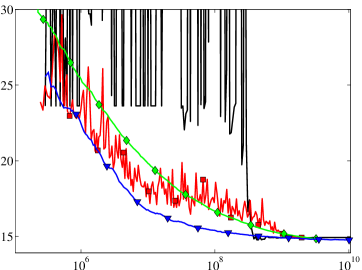
	Kernel Evaluations	Kernel Evaluations

	MNIST
Test error
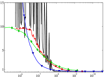
	Kernel Evaluations

Figure 2.8: Classification error on the held-out testing set (linear scale) vs. the number of kernel evaluations performed during optimization (log scale), averaged over ten runs All algorithms were run for ten epochs.

We first compared the methods on a SVM formulation without an unregularized bias, since Pegasos and SDCA do not naturally handle one. So that this comparison would be implementation-independent, we measure performance in terms of the number of kernel evaluations. As can be seen in Figure 2.8, the SBP outperforms Pegasos and SDCA, as predicted by the upper bounds. The SMO algorithm has a dramatically different performance profile, in line with the known analysis: it makes relatively little progress, in terms of generalization error, until it reaches a certain critical point, after which it converges rapidly. Unlike the other methods, terminating SMO early in order to obtain a cruder solution does not appear to be advisable.

To give a sense of actual runtime, we compared our implementation of the SBP to the SVM package LibSVM, running on an Intel E7500 processor. We allowed an unregularized bias (since that is what LibSVM uses), and used the parameters in Table 2.7. For these experiments, we replaced the Reuters dataset with the version of the Forest dataset used by Nguyen et al. [42], using their parameters. LibSVM (with default optimization parameters, except that “shrinking” was turned off) converged to a solution with $14.9$% error in $195$s on Adult, $0.44$% in $1980$s on MNIST, and $1.8$% in $35$ hours on Forest. In one-quarter of each of these runtimes, SBP obtained $15.0$% error on Adult, $0.46$% on MNIST, and $1.6$% on Forest. These results of course depend heavily on the specific stopping criterion used by LibSVM, and do not directly compare the runtimes required to reach solutions which generalize well. We refer to the experiments discussed above for a more controlled comparison. When comparing these SBP results to those of our own SMO implementation, it appears to us that the SBP converges to an acceptable solution more rapidly on Adult, but more slowly on Reuters and MNIST.

11.1   Perceptron

	Reuters	Adult
Test error
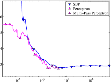
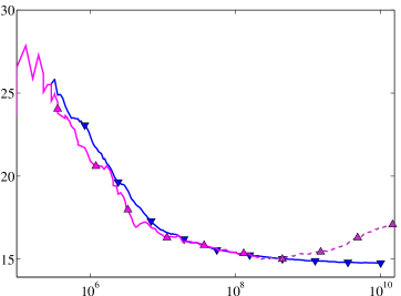
	Inner Products	Inner Products

	MNIST
Test error
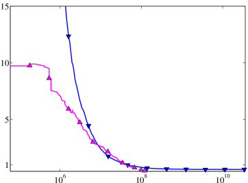
	Inner Products

Figure 2.9: Classification error on the held-out testing set (linear scale) vs. the number of kernel evaluations performed during optimization (log scale), averaged over ten runs. The Perceptron was run for multiple passes over the data—its curve becomes dashed after the first epoch ($n$ iterations). All algorithms were run for ten epochs, except for Perceptron on Adult, which we ran for $100$ epochs to better illustrate its overfitting.

We also compared to the online Perceptron algorithm. As can be seen in Figure 2.9, the Perceptron’s generalization performance is similar to that of the SBP for the first epoch (light purple curve), but the SBP continues improving over additional passes. Although use of the Perceptron is justified for non-separable data only if run for a single pass over the training set, we did continue running for multiple passes (dark purple curve). This is unsafe, since it might overfit after the first epoch, an effect which is clearly visible on the Adult dataset.

11.2   Random Projections

	Reuters	Adult
Test error
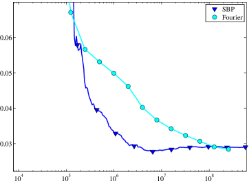
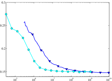
	Inner Products	Inner Products

	MNIST
Test error
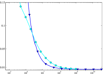
	Inner Products

Figure 2.10: Classification error on the held-out testing set (linear scale) vs. computational cost measured in units of $d$-dimensional inner products (where the training vectors satisfy $x\in\mathbb{R}^{d}$) (log scale), and averaged over ten runs. For the Fourier features, the computational cost (horizontal axis) is that of computing $k\in\left\{1,2,4,8,\dots\right\}$ pairs of Fourier features over the entire training set, while the test error is that of the optimal classifier trained on the resulting linearized SVM objective.

Our final set of experiments compares to the random Fourier projection approach of Rahimi and Recht [47]. Figure 2.10 compares the computational cost of the use of Fourier features to that of the SBP in terms of $d$-dimensional inner products. In this figure, the computational cost of a $2k$-dimensional Fourier linearization is taken to be the cost of computing $\mathcal{P}\left(x_{i}\right)$ on the entire training set ($kn$ inner products, where $n$ is the number of training examples)—we ignore the cost of optimizing the resulting linear SVM entirely. The plotted testing error is that of the optimum of the resulting linear SVM problem, which approximates the original kernel SVM. We can see that at least on Reuters and MNIST, the SBP is preferable to (i.e. faster than) approximating the kernel with random Fourier features.

Collaborators:

The work presented in this chapter was performed jointly with Shai Shalev-Shwartz and Nathan Srebro.

12   Proofs for Chapter 2

lem:svm-sbp:slack-constrained-supergradient

For any $w$, let $p^{*},\xi^{*}$ be minimax optimal for Equation 2.3. Then $\sum_{i=1}^{n}p^{*}_{i}y_{i}\Phi\left(x_{i}\right)$ is a supergradient of $f(w)$ at $w$.

By the definition of $f$, for any $v\in\mathbb{R}^{d}$:

$$f\left(w+v\right)=\max_{\xi\succeq 0,\mathbf{1}^{T}\xi\leq n\nu}\min_{p\in\Delta^{n}}\sum_{i=1}^{n}p_{i}\left(y_{i}\left\langle{w+v},{\Phi\left(x_{i}\right)}\right\rangle+\xi_{i}\right)$$

Substituting the particular value $p^{*}$ for $p$ can only increase the RHS, so:

$$f\left(w+v\right)\leq \max_{\xi\succeq 0,\mathbf{1}^{T}\xi\leq n\nu}\sum_{i=1}^{n}p^{*}_{i}\left(y_{i}\left\langle{w+v},{\Phi\left(x_{i}\right)}\right\rangle+\xi_{i}\right)$$

$$\leq \max_{\xi\succeq 0,\mathbf{1}^{T}\xi\leq n\nu}\sum_{i=1}^{n}p^{*}_{i}\left(y_{i}\left\langle{w},{\Phi\left(x_{i}\right)}\right\rangle+\xi_{i}\right)+\sum_{i=1}^{n}p^{*}_{i}y_{i}\left\langle{v},{\Phi\left(x_{i}\right)}\right\rangle$$

Because $p^{*}$ is minimax-optimal at $w$:

$$f\left(w+v\right)\leq f\left(w\right)+\sum_{i=1}^{n}p^{*}_{i}y_{i}\left\langle{v},{\Phi\left(x_{i}\right)}\right\rangle$$

$$\leq f\left(w\right)+\left\langle{v},{\sum_{i=1}^{n}p^{*}_{i}y_{i}\Phi\left(x_{i}\right)}\right\rangle$$

So $\sum_{i=1}^{n}p^{*}_{i}y_{i}\Phi\left(x_{i}\right)$ is a supergradient of $f$. lem:svm-sbp:zinkevich-batch

For any $T,\delta>0$, after $T$ iterations of the Stochastic Batch Perceptron, with probability at least $1-\delta$, the average iterate $\bar{w}=\frac{1}{T}\sum_{t=1}^{T}w^{(t)}$ (corresponding to $\bar{\alpha}=\frac{1}{T}\sum_{t=1}^{T}\alpha^{(t)}$), satisfies: $f\left(\bar{w}\right)\geq\sup_{\left\lVert{w}\right\rVert\leq 1}f\left(w\right)-O\left(\sqrt{\frac{1}{T}\log\frac{1}{\delta}}\right).$

Define $h=-\frac{1}{r}f$, where $f$ is as in Equation 2.3. Then the stated update rules constitute an instance of Zinkevich’s algorithm, in which steps are taken in the direction of stochastic subgradients $g^{(t)}$ of $h$ at $w^{(t)}=\sum_{i=1}^{n}\alpha_{i}y_{i}\Phi\left(x_{i}\right)$.

The claimed result follows directly from Zinkevich [66, Theorem 1] combined with an online-to-batch conversion analysis in the style of Cesa-Bianchi et al. [11, Lemma 1]. thm:svm-sbp:slack-constrained-runtime

Let $u$ be an arbitrary linear classifier in the RKHS and let $\epsilon>0$ be given. There exist values of the training size $n$, iteration count $T$ and parameter $\nu$ such that Algorithm 2.3 finds a solution $w=\sum_{i=1}^{n}\alpha_{i}y_{i}\Phi\left(x_{i}\right)$ satisfying:

$$\mathcal{L}_{\mathrm{0/1}}\left(g_{w}\right)\leq\mathcal{L}_{\mathrm{hinge}}\left(g_{u}\right)+\epsilon$$

where $\mathcal{L}_{\mathrm{0/1}}\left(g_{w}\right)$ and $\mathcal{L}_{\mathrm{hinge}}\left(g_{u}\right)$ are the expected 0/1 and hinge losses, respectively, after performing the following number of kernel evaluations:

$$\mbox{\#K}=\tilde{O}\left(\left(\frac{\mathcal{L}_{\mathrm{hinge}}\left(g_{u}\right)+\epsilon}{\epsilon}\right)^{3}\frac{\left\lVert{u}\right\rVert^{4}}{\epsilon}\log^{2}\frac{1}{\delta}\right)$$

with the size of the support set of $w$ (the number nonzero elements in $\alpha$) satisfying:

$$\mbox{\#S}=O\left(\left(\frac{\mathcal{L}_{\mathrm{hinge}}\left(g_{u}\right)+\epsilon}{\epsilon}\right)^{2}\left\lVert{u}\right\rVert^{2}\log\frac{1}{\delta}\right)$$

the above statements holding with probability $1-\delta$.

For a training set of size $n$, where:

$$n=\tilde{O}\left(\left(\frac{\mathcal{L}_{\mathrm{hinge}}\left(g_{u}\right)+\epsilon}{\epsilon}\right)\frac{B^{2}}{\epsilon}\log\frac{1}{\delta}\right)$$

taking $B=2\left\lVert{u}\right\rVert$ in Lemma LABEL:lem:svm-introduction:generalization-from-expected-loss gives that $\hat{\mathcal{L}}_{\mathrm{hinge}}\left(g_{u}\right)\leq\mathcal{L}_{\mathrm{hinge}}\left(g_{u}\right)+\epsilon$ and $\mathcal{L}_{\mathrm{0/1}}\left(g_{w}\right)\leq\mathcal{L}_{\mathrm{hinge}}\left(g_{u}\right)+2\epsilon$ with probability $1-\delta$ over the training sample, uniformly for all linear classifiers $w$ such that $\left\lVert{w}\right\rVert\leq B$ and $\hat{\mathcal{L}}_{\mathrm{hinge}}\left(g_{w}\right)-\hat{\mathcal{L}}_{\mathrm{hinge}}\left(g_{u}\right)\leq\epsilon$. We will now show that these inequalities are satisfied by the result of Algorithm 2.3. Define:

$$\hat{w}^{*}=\underset{w:\left\lVert{w}\right\rVert\leq\left\lVert{u}\right\rVert}{\operatorname{argmin}}\hat{\mathcal{L}}_{\mathrm{hinge}}\left(g_{w}\right)$$

Because $\hat{w}^{*}$ is a Pareto optimal solution of the bi-criterion objective of Problem 1.1, if we choose the parameter $\nu$ to the slack-constrained objective (Problem 2.1) such that $\left\lVert{\hat{w}^{*}}\right\rVert\nu=\hat{\mathcal{L}}_{\mathrm{hinge}}\left(g_{\hat{w}^{*}}\right)$, then the optimum of the slack-constrained objective will be equivalent to $\hat{w}^{*}$ (Lemma 2.2). As was discussed in Section 9.4, We will use Lemma LABEL:lem:svm-sbp:zinkevich-batch to find the number of iterations $T$ required to satisfy Equation 2.7 (with $u=\hat{w}^{*}$). This yields that, if we perform $T$ iterations of Algorithm 2.3, where $T$ satisfies the following:

$$T\geq O\left(\left(\frac{\hat{\mathcal{L}}_{\mathrm{hinge}}\left(g_{\hat{w}^{*}}\right)+\epsilon}{\epsilon}\right)^{2}\left\lVert{\hat{w}^{*}}\right\rVert^{2}\log\frac{1}{\delta}\right)$$ (2.12)

then the resulting solution $w=\bar{w}/\gamma$ will satisfy:

$$\left\lVert{w}\right\rVert \leq 2\left\lVert{\hat{w}^{*}}\right\rVert$$

$$\hat{\mathcal{L}}_{\mathrm{hinge}}\left(g_{w}\right)-\hat{\mathcal{L}}_{\mathrm{hinge}}\left(g_{\hat{w}^{*}}\right) \leq\epsilon$$

with probability $1-\delta$. That is:

$$\left\lVert{w}\right\rVert \leq 2\left\lVert{\hat{w}^{*}}\right\rVert$$

$$\leq B$$

and:

$$\hat{\mathcal{L}}_{\mathrm{hinge}}\left(g_{w}\right) \leq\hat{\mathcal{L}}_{\mathrm{hinge}}\left(g_{\hat{w}^{*}}\right)+\epsilon$$

$$\leq\hat{\mathcal{L}}_{\mathrm{hinge}}\left(g_{u}\right)+\epsilon$$

These are precisely the bounds on $\left\lVert{w}\right\rVert$ and $\hat{\mathcal{L}}_{\mathrm{hinge}}\left(g_{w}\right)$ which we determined (at the start of the proof) to be necessary to permit us to apply Lemma LABEL:lem:svm-introduction:generalization-from-expected-loss. Each of the $T$ iterations requires $n$ kernel evaluations, so the product of the bounds on $T$ and $n$ bounds the number of kernel evaluations (we may express Equation 2.12 in terms of $\mathcal{L}_{\mathrm{hinge}}\left(g_{u}\right)$ and $\left\lVert{u}\right\rVert$ instead of $\hat{\mathcal{L}}_{\mathrm{hinge}}\left(g_{\hat{w}^{*}}\right)$ and $\left\lVert{\hat{w}^{*}}\right\rVert$, since $\hat{\mathcal{L}}_{\mathrm{hinge}}\left(g_{\hat{w}^{*}}\right)\leq\hat{\mathcal{L}}_{\mathrm{hinge}}\left(g_{u}\right)\leq\mathcal{L}_{\mathrm{hinge}}\left(g_{u}\right)+\epsilon$ and $\left\lVert{\hat{w}^{*}}\right\rVert\leq\left\lVert{u}\right\rVert$).

Because each iteration will add at most one new element to the support set, the size of the support set is bounded by the number of iterations, $T$.

This discussion has proved that we can achieve suboptimality $2\epsilon$ with probability $1-2\delta$ with the given #K and #S. Because scaling $\epsilon$ and $\delta$ by $1/2$ only changes the resulting bounds by constant factors, these results apply equally well for suboptimality $\epsilon$ with probability $1-\delta$.

Learning Optimally Sparse Support Vector Machines

13   Overview

In the previous chapter, we presented a kernel SVM optimization algorithm with the best known bound on its training runtime. In this chapter, we will consider the related problem of testing runtime. The approach which we describe, which was originally presented in the 29th International Conference on Machine Learning (ICML 2013) [19], results in the best known bound on the testing runtime of the learned predictor. This is possible because the predictor can be expressed in terms of only a subset of the training points, known as “support vectors”. The number of support vectors determines the memory footprint of the learned predictor, as well as the computational cost of using it (i.e. of classifying query points). In order for SVMs to be practical in large scale applications, it is therefore important to have only a small number of support vectors. This is particularly true when, as is the case in many applications, the training is done only once, on a powerful compute cluster that can handle large data, but the predictor then needs to be used many times, possibly in real time, perhaps on a small low-powered device.

However, when training a SVM in the non-separable setting, all incorrectly classified points will be support vectors—e.g. with 10% error, the solution of the SVM empirical optimization problem will necessarily have at least 10% of the training points as support vectors. For data sets with many thousands or even millions of points, this results in very large predictors that are expensive to store and use. Even for some separable problems, the number of support vectors in the SVM solution (the margin-maximizing classifier) may increase linearly with the training set size (e.g. when all the points are on the margin). And so, even though minimizing the empirical SVM objective might be good in terms of generalization ability (and this is very well studied), as we argue here, it might be bad in terms of obtaining sparse solutions.

In this paper, we ask how sparse a predictor we can expect, and show how to learn a SVM predictor with an optimal guarantee on its sparsity, without increasing the required sample complexity nor (asymptotically) the training runtime, and for which the worst-case generalization error has the same bound as the best known for (non-sparse) kernel SVM optimization.

14   Sparse SVMs

In this work, we’re interested in the problem of finding sparse SVM solutions. Hence, the question is whether, given that there exists a good reference classifier $u$ which does not necessarily have a small support size, it is possible to efficiently find a $w$ based on a training sample which not only generalizes well, but also has a small support set.

If the reference classifier $u$ separates the data with a margin, namely $\mathcal{L}_{\mathrm{hinge}}\left(g_{u}\right)=0$, then one can run the kernelized Perceptron algorithm (see for example Freund and Schapire [22]). The Perceptron processes the training examples one by one and adds a support vector only when it makes a prediction mistake. Therefore, a bound on the number of prediction mistakes (i.e. a mistake bound) translates to a bound on the sparsity of the learned predictor. A classic result (the mistake bound used to prove Lemma LABEL:thm:svm-sbp:perceptron-runtime in Chapter 1) shows that if the data is separable with a margin $1$ by some vector $u$, then the Perceptron will make at most $\left\lVert{u}\right\rVert^{2}$ prediction mistakes. Combining this with a generalization bound based on compression of representation (or with an online-to-batch conversion) we can conclude that with $n\geq\tilde{O}(\left\lVert{u}\right\rVert^{2}/\epsilon)$, the generalization error of $w$ will be at most $\epsilon$.

The non-separable case is more tricky. If we somehow obtained a vector $v$ which makes a small number of margin violations on the training set, i.e. $\epsilon_{v}=\frac{1}{n}\sum_{i=1}^{n}\mathbf{1}(y_{i}\left\langle{v},{\Phi(x_{i})}\right\rangle<1)$ is small, then we can find a $w$ with $\left\lVert{v}\right\rVert^{2}$ support vectors which satisfies $\hat{\mathcal{L}}_{\mathrm{0/1}}\left(g_{w}\right)\leq\epsilon_{v}$ by simply ignoring the examples on which $y_{i}\left\langle{v},{\Phi(x_{i})}\right\rangle<1$ and running the Perceptron on the remainder. Again using a compression bound, we can show that $\mathcal{L}_{\mathrm{0/1}}\left(g_{w}\right)$ is little larger than $\hat{\mathcal{L}}_{\mathrm{0/1}}\left(g_{w}\right)$.

However, we cannot, in general, efficiently find a predictor $v$ with a low margin error rate, even if we know that such a predictor exists. Instead, in learning SVMs, we minimize the empirical hinge loss. It is not clear how to relate the margin error rate $\epsilon_{v}$ to the hinge loss of $u$. One option is to note that $\mathbf{1}(z<1)\leq 2[1-z/2]_{+}$, hence $\epsilon_{v}\leq 2\hat{\mathcal{L}}_{\mathrm{hinge}}\left(g_{v/2}\right)$. Since $2\hat{\mathcal{L}}_{\mathrm{hinge}}\left(g_{v/2}\right)$ is a convex function of $v$, we can minimize it as a convex surrogate to $\epsilon_{v}$. Unfortunately, this approach would lead to a dependence on the quantity $2\mathcal{L}_{\mathrm{hinge}}\left(g_{u/2}\right)$, which might be significantly larger than $\mathcal{L}_{\mathrm{hinge}}\left(g_{u}\right)$. This is the main issue we address in Section 15, in which we show how to construct an efficient sparsification procedure which depends on $\mathcal{L}_{\mathrm{hinge}}\left(g_{u}\right)$ and has the same error guarantees and sample complexity as the vanilla SVM predictor.

Before moving on, let us ask whether we could hope for sparsity less then $\Theta(\left\lVert{u}\right\rVert^{2})$. As the following Lemma establishes, we cannot:

lem:svm-sparse:lower-bound

Let $R,\mathcal{L}^{*},\epsilon\geq 0$ be given, with $\mathcal{L}^{*}+\epsilon\leq\nicefrac{{1}}{{4}}$ and with $R^{2}$ being an integer. There exists a data distribution $\mathcal{D}$ and a reference vector $u$ such that $\left\lVert{u}\right\rVert=R$, $\mathcal{L}_{\mathrm{hinge}}\left(g_{u}\right)=\mathcal{L}^{*}$, and any $w$ which satisfies:

$$\mathcal{L}_{\mathrm{0/1}}\left(g_{w}\right)\leq\mathcal{L}^{*}+\epsilon$$

must necessarily be supported on at least $R^{2}/2$ vectors. Furthermore, the claim also holds for randomized classification rules that predict $1$ with probability $\psi(g_{u}(x))$ for some $\psi:\mathbb{R}\to[0,1]$.

We define $\mathcal{D}$ such that $i$ is sampled uniformly at random from the set $\left\{1,\dots,d\right\}$, with $d=R^{2}$, and the feature vector is taken to be $x=e_{i}$ (the $i$th standard unit basis vector) with corresponding label distributed according to $\mathrm{Pr}\left\{y=z\right\}=1-\mathcal{L}^{*}/2$. The value of $z\in\{\pm 1\}$ will be specified later. Choose ${u}_{i}=z$ for all $i$, so that $\left\lVert{u}\right\rVert=R$ and $\mathcal{L}_{\mathrm{hinge}}\left(g_{u}\right)=\mathcal{L}^{*}$.

Take $w$ to be a linear combination of $k<d/2=R^{2}/2$ vectors. Then $g_{w}(x)=0$ on any $x$ which is not in its support set. Suppose that whenever $g_{w}(x_{i})=0$ the algorithm predicts the label $1$ with probability $p\in[0,1]$ ($p=\psi(0)$ for a randomized classifier). If $p\geq 1/2$ we’ll set $z=-1$, and if $p<1/2$ we’ll set $z=1$. This implies that:

$$\mathcal{L}_{\mathrm{0/1}}\left(g_{w}\right)\geq\frac{d-k}{2d}>\frac{1}{4}\geq\mathcal{L}^{*}+\epsilon$$

which concludes the proof.

15   Learning Sparse SVMs

In the previous section we showed that having a good low-norm predictor $u$ often implies there exists also a good sparse predictor, but the existence proof required low margin error. We will now consider the problem of efficiently finding a good sparse predictor, given the existence of low-norm reference predictor $u$ which suffers low hinge loss on a finite training sample.

Our basic approach will be broadly similar to that of Section 14, but instead of relying on an unknown $u$, we will start by using any SVM optimization approach to learn a (possibly dense) $w$. We will then learn a sparse classifier $\tilde{w}$ which mimics $w$.

In Section 14 we removed margin violations and dealt with an essentially separable problem. But when one considers not margin error, but hinge loss, the difference between “correct” and “wrong” is more nuanced, and we must take into account the numeric value of the loss:

1. If $y\left\langle{w},{\Phi(x)}\right\rangle\leq 0$ (i.e. $w$ is wrong), then we can ignore the example, as in Section 14.

2. If $0<y\left\langle{w},{\Phi(x)}\right\rangle<1$ (i.e. $w$ is correct, but there is a margin violation), then we allow $\tilde{w}$ to make a margin violation at most $\nicefrac{{1}}{{2}}$ worse than the margin violation made by $w$, i.e. $y\left\langle{\tilde{w}},{\Phi(x)}\right\rangle\geq y\left\langle{w},{\Phi(x)}\right\rangle-\nicefrac{{1}}{{2}}$.

3. If $y\left\langle{w},{\Phi(x)}\right\rangle\geq 1$ (i.e. $w$ is correct and classifies this example outside the margin), we would like $\tilde{w}$ to also be correct, though we require a smaller margin: $y\left\langle{\tilde{w}},{\Phi(x)}\right\rangle\geq\nicefrac{{1}}{{2}}$.

These are equivalent to finding a solution with value at most $\nicefrac{{1}}{{2}}$ to the following optimization problem:

$$\text{minimize}: f(\tilde{w})=\max_{i:h_{i}>0}\left(h_{i}-y_{i}\left\langle{\tilde{w}},{\Phi(x_{i})}\right\rangle\right)$$ (3.1)

$$\text{where}: h_{i}=\min\left(1,y_{i}\left\langle{w},{\Phi(x_{i})}\right\rangle\right)$$

We will show that a randomized classifier based on a solution to Problem 3.1 with $f\left(\tilde{w}\right)\leq\nicefrac{{1}}{{2}}$ has empirical 0/1 error bounded by the empirical hinge loss of $w$; that we can efficiently find such solution based on at most $4\left\lVert{w}\right\rVert^{2}$ support vectors; and that such a sparse solution generalizes as well as $w$ itself.

15.1   The Slant-loss

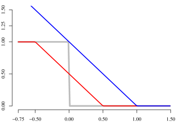
Figure 3.1: Illustration of how the slant-loss (red) relates to the 0/1 (gray) and hinge (blue) losses. Notice that, if the slant-loss is shifted by $\nicefrac{{1}}{{2}}$, then it is still upper bounded by the hinge loss.

The key to our approach is our use of the randomized classification rule $\tilde{g}_{\tilde{w}}\left(x\right)=\left\langle{\tilde{w}},{\Phi\left(x\right)}\right\rangle+Z$ for $Z\sim\mbox{Unif}\left[-\nicefrac{{1}}{{2}},\nicefrac{{1}}{{2}}\right]$, rather than the standard linear classification rule $g_{w}\left(x\right)=\left\langle{w},{\Phi\left(x\right)}\right\rangle$. The effect of the randomization is to “spread out” the expected loss of the classifier. We define the loss function:

$$\ell_{slant}\left(z\right)=\min\left(1,\max\left(0,\nicefrac{{1}}{{2}}-z\right)\right)$$ (3.2)

which we call the “slant-loss” (Figure 3.1), using $\mathcal{L}_{\mathrm{slant}}\left(g\right)$ and $\hat{\mathcal{L}}_{\mathrm{slant}}\left(g\right)$ to denote its expectation and empirical average, analogously to the 0/1 and hinge losses. It is easy to see that $\mathbb{E}_{Z}\left[\ell_{0/1}(\tilde{g}_{\tilde{w}})\right]=\ell_{slant}(g_{\tilde{w}})$—hence, the $0/1$ loss of $\tilde{g}_{\tilde{w}}$ is the same as the slant-loss of $g_{\tilde{w}}$. Equally importantly, $\ell_{slant}(z-\nicefrac{{1}}{{2}})\leq\ell_{hinge}(z)$, from which the following Lemma follows:

lem:svm-sparse:slant-loss

For any $w$, and any $\tilde{w}$ for which Problem 3.1 has value $f\left(\tilde{w}\right)\leq\nicefrac{{1}}{{2}}$, we have that

$$\mathbb{E}_{Z}\left[\hat{\mathcal{L}}_{0/1}\left(\tilde{g}_{\tilde{w}}\right)\right]=\hat{\mathcal{L}}_{slant}\left(g_{\tilde{w}}\right)\leq\hat{\mathcal{L}}_{hinge}\left(g_{w}\right)$$

It remains only to establish that $\hat{\mathcal{L}}_{slant}\left(g_{\tilde{w}}\right)\leq\hat{\mathcal{L}}_{hinge}\left(g_{w}\right)$. For every $x_{i},y_{i}$, consider the following three cases:

1. If $y_{i}\left\langle{w},{\Phi(x_{i})}\right\rangle\leq 0$, then $\ell_{slant}(y_{i}g_{\tilde{w}}(x_{i}))\leq 1\leq\ell_{hinge}(y_{i}g_{w}(x_{i}))$.

2. If $0<y_{i}\left\langle{w},{\Phi(x_{i})}\right\rangle<1$, then $\ell_{slant}(y_{i}g_{\tilde{w}}(x_{i}))\leq\ell_{slant}(y_{i}g_{w}(x_{i})-\nicefrac{{1}}{{2}})\leq\ell_{hinge}(y_{i}g_{w}(x_{i}))$.

3. If $y_{i}\left\langle{w},{\Phi(x_{i})}\right\rangle\geq 1$, then $\ell_{slant}(y_{i}g_{\tilde{w}}(x_{i}))\leq\ell_{slant}(\nicefrac{{1}}{{2}})=0=\ell_{hinge}(y_{i}g_{w}(x_{i}))$.

Hence, $\ell_{slant}(y_{i}g_{\tilde{w}}(x_{i}))\leq\ell_{hinge}(y_{i}g_{w}(x_{i}))$, which completes the proof.

15.2   Finding Sparse Solutions

$\mbox{{optimize}}\left(n:\mathbb{N},d:\mathbb{N},x_{1},\dots,x_{n}:\mathbb{R}^{d},y_{1},\dots,y_{n}:\left\{\pm 1\right\},h:\mathbb{R}^{n},K:\mathbb{R}^{d}\times\mathbb{R}^{d}\rightarrow\mathbb{R}_{+}\right)$
1	$\eta:=1/2$; $\tilde{\alpha}^{(0)}:=0^{n}$; $\tilde{c}^{(0)}:=0^{n}$;
2	do
3		$i:=\operatorname{argmax}_{i:h_{i}>0}\left(h_{i}-\tilde{c}_{i}\right)$;
4		$\mbox{{if }}h_{i}-\tilde{c}_{i}\leq 1/2\mbox{{ then}}$
5			$\mbox{{return }}\tilde{\alpha}$;
6		$\tilde{\alpha}^{(t)}:=\tilde{\alpha}^{(t-1)}+\eta e_{i}$;
7		$\mbox{{for }}j=1\mbox{{ to }}n$
8			$\tilde{c}^{(t)}_{j}:=\tilde{c}^{(t-1)}_{j}+\eta y_{i}y_{j}K\left(x_{i},x_{j}\right)$;

Algorithm 3.2 Subgradient ascent algorithm for optimizing the kernelized version of Problem 3.1. Here, $\tilde{\alpha}$ is the vector of coefficients representing $\tilde{w}$ as a linear combination of the training data: $\tilde{w}=\sum_{i=1}^{n}\tilde{\alpha}_{i}y_{i}\Phi\left(x_{i}\right)$ (this is the representor theorem—see Section 2 of Chapter 1). The vector $h$ is derived from the initial SVM solution as in Problem 3.1, and $e_{i}$ is the $i$th standard unit basis vector. Lemma LABEL:lem:svm-sparse:convergence-rate shows that the termination condition on line $4$ will be satisfied after at most $4\left\lVert{w}\right\rVert^{2}$ iterations.

To find a sparse $\tilde{w}$ with value $f(\tilde{w})\leq 1/2$, we apply subgradient descent to Problem 3.1. The algorithm is extremely straightforward to understand and implement. We initialize $\tilde{w}^{(0)}=0$, and then proceed iteratively, performing the following at the $t$th iteration:

1. Find the training index $i:y_{i}\left\langle{w},{\Phi(x_{i})}\right\rangle>0$ which maximizes $h_{i}-y_{i}\left\langle{\tilde{w}^{(t-1)}},{\Phi(x_{i})}\right\rangle$.

2. Take the subgradient step $\tilde{w}^{(t)}\leftarrow\tilde{w}^{(t-1)}+\eta y_{i}\Phi(x_{i})$.

To this point, we have worked in the explicit kernel Hilbert space $\mathcal{H}$, even though we are interested primarily in the kernelized case, where $\mathcal{H}$ and $\Phi(\cdot)$ are specified only implicitly through $K(x,x^{\prime})=\left\langle{\Phi(x)},{\Phi(x^{\prime})}\right\rangle$. However, like the SBP (Chapter 2), the above algorithm can be interpreted as an instance of the traditional SVM optimization outline of Section 4 in Chapter 1, by relying on the representations $w=\sum_{i=1}^{n}\alpha_{i}y_{i}\Phi(x_{i})$ and $\tilde{w}=\sum_{i=1}^{n}\tilde{\alpha}_{i}y_{i}\Phi(x_{i})$, keeping track of the coefficients $\alpha$ and $\tilde{\alpha}$. We will also maintain an up-to-date vector of responses $\tilde{c}$:

$$\tilde{c}_{j}=y_{j}\left\langle{\tilde{w}},{\Phi(x_{j})}\right\rangle=\sum_{i=1}^{n}\tilde{\alpha}_{i}y_{i}y_{j}K(x_{i},x_{j})$$

Notice that the values of the responses provide sufficient knowledge to find the update index $i$ at every iteration. We can then perform the subgradient descent update $\tilde{w}\leftarrow\tilde{w}+\eta y_{i}\Phi(x_{i})$ by adding $\eta$ to $\tilde{\alpha}_{i}$, and updating the responses as $\tilde{c}_{j}\leftarrow\tilde{c}_{j}+\eta y_{i}y_{j}K(x_{i},x_{j})$, at a total cost of $n$ kernel evaluations.

Algorithm 3.2 gives a detailed version of this algorithm, as an instance of the outline of Algorithm 4. Its convergence rate is characterized in the following lemma:

lem:svm-sparse:convergence-rate

After $T\leq 4\left\lVert{w}\right\rVert^{2}$ iterations of subgradient descent with $\eta=\nicefrac{{1}}{{2}}$, we obtain a solution of the form $\tilde{w}=\frac{1}{2}\sum_{t=1}^{T}y_{i_{t}}\Phi(x_{i_{t}})$ which has value $f\left(\tilde{w}\right)\leq\nicefrac{{1}}{{2}}$.

First note that $f(w)\leq 0$. Relying on this possible solution $w$, the Lemma follows from standard convergence bounds of subgradient descent (see e.g. Section 1.2 of Nesterov [41]): with the step size $\eta=\epsilon$, after performing $\left\lVert{w}\right\rVert^{2}/\epsilon^{2}$ iterations, at least one iterate $\tilde{w}^{(t)}$ will have an objective function value no greater than $\epsilon$. Choosing $\epsilon=\nicefrac{{1}}{{2}}$ gives the desired result. Because each iteration adds at most one new element to the support set, the support size of the solution will likewise be bounded by $4\left\lVert{w}\right\rVert^{2}$. We must calculate the objective function value in the course of each subgradient descent iteration (while finding $i$), so one can identify an iterate with $f(\tilde{w}^{(t)})\leq\nicefrac{{1}}{{2}}$ at no additional cost—this is the termination condition on line $4$ of Algorithm 3.2.

15.3   Generalization Guarantee - Compression

The fact that the optimization procedure outlined in the previous section results in a sparse predictor of a particularly simple structure enables us to bound its generalization error using a compression bound. Before giving our generalization bound, we begin by presenting the compression bound which we use:

thm:svm-sparse:compression-bound

This is Theorem 2 of Shalev-Shwartz [50]. Let $k$ and $n$ be fixed, with $n\geq 2k$, and let $A:\left(\mathbb{R}^{d}\times\left\{\pm 1\right\}\right)^{k}\rightarrow\mathcal{H}$ be a mapping which receives a list of $k$ labeled training examples, and returns a classification vector $w\in\mathcal{H}$. Use $S\in\left[n\right]^{k}$ to denote a list of $k$ training indices, and let $w_{S}$ be the result of applying $A$ to the training elements indexed by $S$. Finally, let $\ell:\mathbb{R}\rightarrow\left[0,1\right]$ be a loss function bounded below by $0$ and above by $1$, with $\mathcal{L}\left(g_{w}\right)$ and $\hat{\mathcal{L}}\left(g_{w}\right)$ the expected loss, and empirical loss on the training set, respectively. Then, with probability $1-\delta$, for all $S$:

$$\mathcal{L}\left(g_{w_{S}}\right)\leq\hat{\mathcal{L}}\left(g_{w_{S}}\right)+\sqrt{\frac{32\hat{\mathcal{L}}\left(g_{w_{S}}\right)\left(k\log n+\log\frac{1}{\delta}\right)}{n}}+\frac{8\left(k\log n+\log\frac{1}{\delta}\right)}{n}$$

Consider, for some fixed $\delta^{\prime}$, the probability that there exists a $S\subseteq\left\{1,\dots,n\right\}$ of size $k$ such that:

$$\mathcal{L}\left(g_{w_{S}}\right)\geq\hat{\mathcal{L}}_{\mbox{test}}\left(g_{w_{S}}\right)+\sqrt{\frac{2\hat{\mathcal{L}}_{\mbox{test}}\left(g_{w_{S}}\right)\log\frac{1}{\delta^{\prime}}}{\left(n-k\right)}}+\frac{4\log\frac{1}{\delta^{\prime}}}{n-k}$$

where $\hat{\mathcal{L}}_{\mbox{test}}\left(g_{w}\right)=\frac{1}{n-k}\sum_{i\notin S}\ell\left(y_{i}g_{w}\left(x_{i}\right)\right)$ is the empirical loss on the complement of $S$. It follows from Bernstein’s inequality that, for a particular $S$, the above holds with probability at most $\delta^{\prime}$. By the union bound:

$$n^{k}\delta^{\prime}\geq\mathrm{Pr}\left\{\exists S\in[n]^{k}:\mathcal{L}\left(g_{w_{S}}\right)\geq\hat{\mathcal{L}}_{\mbox{test}}\left(g_{w_{S}}\right)+\sqrt{\frac{2\hat{\mathcal{L}}_{\mbox{test}}\left(g_{w_{S}}\right)\log\frac{1}{\delta^{\prime}}}{\left(n-k\right)}}+\frac{4\log\frac{1}{\delta^{\prime}}}{n-k}\right\}$$

Let $\delta=n^{k}\delta^{\prime}$. Notice that $\left(n-k\right)\hat{\mathcal{L}}_{\mbox{test}}\left(g_{w_{S}}\right)\leq n\hat{\mathcal{L}}\left(g_{w_{S}}\right)$, so:

$$\delta\geq\mathrm{Pr}\left\{\exists S\in[n]^{k}:\mathcal{L}\left(g_{w_{S}}\right)\geq\frac{n\hat{\mathcal{L}}\left(g_{w_{S}}\right)}{n-k}+\sqrt{\frac{2n\hat{\mathcal{L}}\left(g_{w_{S}}\right)\log\frac{n^{k}}{\delta}}{\left(n-k\right)^{2}}}+\frac{4\log\frac{n^{k}}{\delta}}{n-k}\right\}$$

Because $\hat{\mathcal{L}}\left(g_{w_{S}}\right)\leq 1$ and $k\leq n$, it follows that $k\hat{\mathcal{L}}\left(g_{w_{S}}\right)\leq 2n\log n$, and therefore that $\frac{k}{n-k}\hat{\mathcal{L}}\left(g_{w_{S}}\right)\leq\sqrt{\frac{2nk\hat{\mathcal{L}}\left(g_{w_{S}}\right)\log n}{\left(n-k\right)^{2}}}\leq\sqrt{\frac{2n\hat{\mathcal{L}}\left(g_{w_{S}}\right)\log\frac{n^{k}}{\delta}}{\left(n-k\right)^{2}}}$. Hence:

$$\delta\geq\mathrm{Pr}\left\{\exists S\in[n]^{k}:\mathcal{L}\left(g_{w_{S}}\right)\geq\hat{\mathcal{L}}\left(g_{w_{S}}\right)+\sqrt{\frac{8n\hat{\mathcal{L}}\left(g_{w_{S}}\right)\log\frac{n^{k}}{\delta}}{\left(n-k\right)^{2}}}+\frac{4\log\frac{n^{k}}{\delta}}{n-k}\right\}$$

Using the assumption that $n\geq 2k$ completes the proof.

With this result in place, it is straightforward to bound the generalization performance of the classifier which is found by our subgradient descent procedure:

lem:svm-sparse:generalization-from-compression

With probability at least $1-\delta$ over the training set, if $\tilde{w}$ is a solution with value $f(\tilde{w})\leq\nicefrac{{1}}{{2}}$ to Problem 3.1 found by performing $T=4\left\lVert{w}\right\rVert^{2}$ iterations of subgradient descent (see Algorithm 3.2 and Lemma LABEL:lem:svm-sparse:convergence-rate), then:

$$\mathcal{L}_{\mathrm{0/1}}\left(\tilde{g}_{\tilde{w}}\right)\leq\hat{\mathcal{L}}_{\mathrm{hinge}}\left(\tilde{g}_{\tilde{w}}\right)+O\left(\sqrt{\hat{\mathcal{L}}_{\mathrm{hinge}}\left(g_{w}\right)\frac{\left\lVert{w}\right\rVert^{2}\log n+\log\frac{1}{\delta}}{n}}+\frac{\left\lVert{w}\right\rVert^{2}\log n+\log\frac{1}{\delta}}{n}\right)$$

provided that $n\geq 2T$.

Because $\tilde{w}$ is found via subgradient descent,it can be written in the form $\tilde{w}=\eta\sum_{i\in S}y_{i}x_{i}=A(S)$ with $S\in\left[n\right]^{k}$, and $k=T=4\left\lVert{w}\right\rVert^{2}$. Hence, by the compression bound of Theorem LABEL:thm:svm-sparse:compression-bound, we have that with probability $1-\delta$:

$$\mathcal{L}_{\mathrm{slant}}\left(g_{\tilde{w}}\right)\leq\hat{\mathcal{L}}_{\mathrm{slant}}\left(g_{\tilde{w}}\right)+\sqrt{\frac{32\hat{\mathcal{L}}_{\mathrm{slant}}\left(g_{\tilde{w}}\right)\left(k\log n+\log\frac{1}{\delta}\right)}{n}}+\frac{8\left(k\log n+\log\frac{1}{\delta}\right)}{n}$$

The randomized classification rule $\tilde{g}_{\tilde{w}}$ was defined in such a way that $\ell_{slant}\left(yg_{\tilde{w}}\left(x\right)\right)=\mathbb{E}\left[\ell_{0/1}\left(y\tilde{g}_{\tilde{w}}\left(x\right)\right)\right]$. Furthermore, as was shown in Lemma LABEL:lem:svm-sparse:slant-loss, $\hat{\mathcal{L}}_{\mathrm{slant}}\left(g_{\tilde{w}}\right)\leq\hat{\mathcal{L}}_{\mathrm{hinge}}\left(g_{w}\right)$. Plugging these results into the above equation:

$$\mathcal{L}_{\mathrm{0/1}}\left(\tilde{g}_{\tilde{w}}\right)\leq\hat{\mathcal{L}}_{\mathrm{hinge}}\left(g_{w}\right)+\sqrt{\frac{32\hat{\mathcal{L}}_{\mathrm{hinge}}\left(g_{w}\right)\left(k\log n+\log\frac{1}{\delta}\right)}{n}}+\frac{8\left(k\log n+\log\frac{1}{\delta}\right)}{n}$$

The above holds for all $w$ such that $\tilde{w}$ is a $\nicefrac{{1}}{{2}}$-suboptimal solution to the corresponding instance of Problem 3.1. Plugging the assumption that $k=4\left\lVert{w}\right\rVert^{2}$ completes the proof.

15.4   Generalization Guarantee - Smoothness

The main disadvantage of using a compression bound to prove generalization is that the result bounds the performance of a particular algorithm (in this case, subgradient descent), instead of the performance of all solutions satisfying some conditions. One can address this drawback by using uniform concentration arguments to obtain an almost identical guarantee (up to log factors) which holds for any $\tilde{w}$ (not necessarily sparse) with norm $\left\lVert{\tilde{w}}\right\rVert\leq\left\lVert{w}\right\rVert$ and value $f(\tilde{w})\leq\nicefrac{{1}}{{3}}$. The result is a bound which is slightly worse than that of Lemma LABEL:lem:svm-sparse:convergence-rate, but is more flexible. In order derive it, we must first modify the objective of Problem 3.1 by adding a norm-constraint:

$$\mbox{minimize}: f(\tilde{w})=\max_{i:y_{i}\left\langle{w},{\Phi(x_{i})}\right\rangle>0}\left(h_{i}-y_{i}\left\langle{\tilde{w}},{\Phi(x_{i})}\right\rangle\right)$$ (3.3)

$$\mbox{subject to}: \left\lVert{\tilde{w}}\right\rVert\leq\left\lVert{w}\right\rVert$$

Here, as before, $h_{i}=\min\left(1,y_{i}\left\langle{w},{\Phi(x_{i})}\right\rangle\right)$. Like Problem 3.1, this objective can be optimized using subgradient descent, although one must add a step in which the current iterate is projected onto the ball of radius $\left\lVert{w}\right\rVert$ after every iteration. Despite this change, an $\epsilon$-suboptimal solution can still be found in $\left\lVert{w}\right\rVert^{2}/\epsilon^{2}$ iterations.

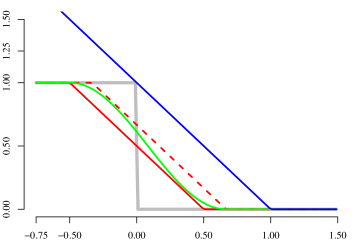
Figure 3.3: Illustration of the how our smooth loss relates to the slant and hinge losses. Our smooth loss (green) upper bounds the slant-loss, and lower bounds the slant-loss when shifted by $\nicefrac{{1}}{{6}}$, and the hinge-loss when shifted by $\nicefrac{{1}}{{3}}$.

The concentration-based version of our main theorem follows:

thm:svm-sparse:main-smooth

Let $R\in\mathbb{R}_{+}$ be fixed. With probability $1-\delta$ over the training sample, uniformly over all pairs $w,\tilde{w}\in\mathcal{H}$ such that $\left\lVert{w}\right\rVert\leq R$ and $\tilde{w}$ has objective function $f(\tilde{w})\leq\nicefrac{{1}}{{3}}$ in Problem 3.3:

$$\mathcal{L}_{\mathrm{0/1}}\left(\tilde{g}_{\tilde{w}}\right)\leq\hat{\mathcal{L}}_{\mathrm{hinge}}\left(g_{w}\right)$$

$$+O\left(\sqrt{\frac{\hat{\mathcal{L}}_{\mathrm{hinge}}\left(g_{w}\right)R^{2}\log^{3}n}{n}}+\sqrt{\frac{\hat{\mathcal{L}}_{\mathrm{hinge}}\left(g_{w}\right)\log\frac{1}{\delta}}{n}}+\frac{R^{2}\log^{3}n}{n}+\frac{\log\frac{1}{\delta}}{n}\right)$$

Because our bound is based on a smooth loss, we begin by defining the bounded $4$-smooth loss $\ell_{smooth}(z)$ to be $1$ if $z<-\nicefrac{{1}}{{2}}$, $0$ if $z>\nicefrac{{2}}{{3}}$, and $\nicefrac{{1}}{{2}}\left(1+\cos\left(\nicefrac{{\pi}}{{2}}\left(1+\nicefrac{{1}}{{7}}\left(12z-1\right)\right)\right)\right)$ otherwise. This function is illustrated in Figure 3.3—notice that it upper-bounds the slant-loss, and lower-bounds the hinge loss even when shifted by $\nicefrac{{1}}{{3}}$. Applying Theorem 1 of Srebro et al. [56] to this smooth loss yields that, with probability $1-\delta$, uniformly over all $\tilde{w}$ such that $\left\lVert{\tilde{w}}\right\rVert\leq R$:

$$\mathcal{L}_{\mathrm{smooth}}\left(g_{\tilde{w}}\right)\leq\hat{\mathcal{L}}_{\mathrm{smooth}}\left(g_{\tilde{w}}\right)+$$

$$O\left(\sqrt{\frac{\hat{\mathcal{L}}_{\mathrm{smooth}}\left(g_{\tilde{w}}\right)R^{2}\log^{3}n}{n}}+\sqrt{\frac{\hat{\mathcal{L}}_{\mathrm{smooth}}\left(g_{\tilde{w}}\right)\log\frac{1}{\delta}}{n}}+\frac{R^{2}\log^{3}n}{n}+\frac{\log\frac{1}{\delta}}{n}\right)$$

Just as the empirical slant-loss of a $\tilde{w}$ with $f(\tilde{w})\leq\nicefrac{{1}}{{2}}$ is upper bounded by the empirical hinge loss of $w$, the empirical smooth loss of a $\tilde{w}$ with $f(\tilde{w})\leq\nicefrac{{1}}{{3}}$ is upper-bounded by the same quantity. As was argued in the proof of Lemma LABEL:lem:svm-sparse:slant-loss, this follows directly from Problem 3.3, and the definition of the smooth loss. Combining this with the facts that the slant-loss lower bounds the smooth loss, and that $\mathcal{L}_{\mathrm{slant}}\left(g_{\tilde{w}}\right)=\mathcal{L}_{\mathrm{0/1}}\left(\tilde{g}_{\tilde{w}}\right)$, completes the proof.

It’s worth pointing out that the addition of a norm-constraint to the objective function (Problem 3.3) is only necessary because we want the theorem to apply to any $\tilde{w}$ with $f(\tilde{w})\leq\nicefrac{{1}}{{3}}$. If we restrict ourselves to $\tilde{w}$ which are found using subgradient descent with the suggested step size and iteration count, then applying the triangle inequality to the sequence of steps yields that $\left\lVert{\tilde{w}}\right\rVert\leq O\left(\left\lVert{w}\right\rVert\right)$, and the above bound still holds (albeit with a different constant hidden inside the big-Oh notation).

15.5   Putting it Together

Now that all of the pieces are in place, we can state our final procedure, start-to-finish:

1. Train a SVM to obtain $w$ with norm $\left\lVert{w}\right\rVert\leq O\left(\left\lVert{u}\right\rVert\right)$ and $\hat{\mathcal{L}}_{\mathrm{hinge}}\left(g_{w}\right)\leq\hat{\mathcal{L}}_{\mathrm{hinge}}\left(g_{u}\right)+O\left(\epsilon\right)$.

2. Run subgradient descent on Problem 3.1 until we find a predictor $\tilde{w}$ with value $f(\tilde{w})\leq\nicefrac{{1}}{{2}}$ (see Algorithm 3.2).

3. Predict using $\tilde{g}_{\tilde{w}}$.

thm:svm-sparse:main-compression

For an arbitrary (unknown) reference classifier $u$, with probability at least $1-2\delta$ over a training set of size:

$$n=\tilde{O}\left(\left(\frac{\mathcal{L}_{\mathrm{hinge}}\left(g_{u}\right)+\epsilon}{\epsilon}\right)\frac{\left\lVert{u}\right\rVert^{2}}{\epsilon}\log\frac{1}{\delta}\right)$$

the procedure above finds a predictor $\tilde{w}$ supported on at most $O(\left\lVert{u}\right\rVert^{2})$ training vectors and error $\mathcal{L}_{\mathrm{0/1}}\left(\tilde{g}_{\tilde{w}}\right)\leq\mathcal{L}_{\mathrm{hinge}}\left(g_{u}\right)+O(\epsilon)$

First, note that with the specified sample size, applying Bernstein’s inequality to the fixed predictor $u$, we have that with probability at least $1-\delta$,

$$\hat{\mathcal{L}}_{\mathrm{hinge}}\left(u\right)\leq\mathcal{L}_{\mathrm{hinge}}\left(u\right)+\epsilon.$$ (3.4)

Combining Equation 3.9 with the SVM training goal (Step 1) and Lemma LABEL:lem:svm-sparse:slant-loss, we have that $\hat{\mathcal{L}}_{\mathrm{slant}}\left(g_{\tilde{w}}\right)\leq\mathcal{L}_{\mathrm{hinge}}\left(g_{u}\right)+O(\epsilon)$. Following Lemma LABEL:lem:svm-sparse:convergence-rate we can apply Lemma LABEL:lem:svm-sparse:generalization-from-compression with $T=O(\|u\|^{2})$, and plugging in the specified sample complexity, we have $\mathcal{L}_{\mathrm{slant}}\left(g_{\tilde{w}}\right)\leq\hat{\mathcal{L}}_{\mathrm{slant}}\left(g_{\tilde{w}}\right)$. Combining the two inequalities, and recalling that the slant-loss of $g_{\tilde{w}}$ is the same as the expected $0/1$ error of $\tilde{g}_{\tilde{w}}$, we obtain $\mathcal{L}_{\mathrm{0/1}}\left(\tilde{g}_{\tilde{w}}\right)\leq\mathcal{L}_{\mathrm{hinge}}\left(g_{u}\right)+O(\epsilon)$. Lemma LABEL:lem:svm-sparse:convergence-rate also establishes the desired bound on the number of support vectors.

The procedure is efficient, and aside from initial SVM optimization, requires at most $O(\left\lVert{u}\right\rVert^{2})$ iterations.

15.6   Kernelization

As we saw in Section 15.2, each iteration of Algorithm 3.2 requires $n$ kernel evaluations. These kernel evaluations dominate the computational cost of the gradient descent procedure (all other operations can be performed in $O(n)$ operations per iteration). As is standard for kernel SVM training, we will therefore analyze runtime in terms of the number of kernel evaluations required.

With $O(\|u\|^{2})$ iterations, and $O(n)$ kernel evaluations per iteration, the overall number of required kernel evaluations for the gradient descent procedure is (ignoring the $\delta$ dependence):

$$O\left(n\left\lVert{u}\right\rVert^{2}\right)=\tilde{O}\left(\left(\frac{\hat{\mathcal{L}}_{\mathrm{hinge}}\left(g_{u}\right)+\epsilon}{\epsilon}\right)\frac{\left\lVert{u}\right\rVert^{4}}{\epsilon}\right)$$

This is less then the best known runtime bound for kernel SVM optimization, so we do not expect the sparsification step to be computationally dominant (i.e. it is in a sense “free”). In order to complete the picture and understand the entire runtime of our method, we must also consider the runtime of the SVM training (Step 1). The best kernelized SVM optimization guarantee of which we are aware is achieved by the Stochastic Batch Perceptron (SBP, Cotter et al. [18]). Using the SBP, we can find $w$ with $\left\lVert{w}\right\rVert\leq 2\left\lVert{u}\right\rVert$ and $\hat{\mathcal{L}}_{\mathrm{hinge}}\left(g_{w}\right)\leq\hat{\mathcal{L}}_{\mathrm{hinge}}\left(g_{u}\right)+\epsilon$ using:

$$O\left(\left(\frac{\hat{\mathcal{L}}_{\mathrm{hinge}}\left(g_{u}\right)+\epsilon}{\epsilon}\right)^{2}\left\lVert{u}\right\rVert^{2}n\right)$$

kernel evaluations, yielding (with the $\delta$-dependence):

Corollary 3.5.

If using the SBP for Step 1 and the sample size required by Theorem LABEL:thm:svm-sparse:main-compression, the procedure in Section 15.5 can be performed with:

$$\tilde{O}\left(\left(\frac{\hat{\mathcal{L}}_{\mathrm{hinge}}\left(g_{u}\right)+\epsilon}{\epsilon}\right)^{3}\frac{\left\lVert{u}\right\rVert^{4}}{\epsilon}\log\frac{1}{\delta}\right)$$

kernel evaluations.

Because the SBP finds a $w$ with $\left\lVert{w}\right\rVert\leq 2\left\lVert{u}\right\rVert$, and our subgradient descent algorithm finds a $\tilde{w}$ supported on $4\left\lVert{w}\right\rVert^{2}$ training vectors, it follows that the support size of $\tilde{w}$ is bounded by $16\left\lVert{u}\right\rVert^{2}$. The runtime of Step 2 (the sparsification procedure) is asymptotically negligible compared to Step 1 (initial SVM training), so the overall runtime is the same as for stand-alone SBP. Overall, our procedure finds an optimally sparse SVM predictor, and at the same time matches the best known sample and runtime complexity guarantees for SVM learning (up to small constant factors).

15.7   Unregularized Bias

Frequently, SVM problems contain an unregularized bias term—rather than the classification function being the sign of $g_{w}(x)=\left\langle{w},{\Phi(x)}\right\rangle$, it is the sign of $g_{w,b}(x)=\left(\left\langle{w},{\Phi(x)}\right\rangle+b\right)$ for a weight vector $w$ and a bias $b$, where the bias is unconstrained, being permitted to take on the value of any real number.

When optimizing SVMs, the inclusion of an unregularized bias introduces some additional complications which typically require special treatment. Our subgradient descent procedure, however, is essentially unchanged by the inclusion of a bias (although the SVM solver which we use to find $w$ and $b$ must account for it). Indeed, we need only redefine:

$$h_{i}=\min\left(1,y_{i}\left(\left\langle{w},{\Phi(x_{i})}\right\rangle+b\right)\right)-y_{i}b$$

in Problem 3.1, and then find $\tilde{w}$ as usual. The resulting sparse classifier is parameterized by $\tilde{w}$ and $b$, with $b$ being that of the initial SVM solution.

Alternatively, instead of taking the bias of the sparse predictor to be the same as that of the original SVM predictor, we may optimize over $\tilde{b}$ during our subgradient descent procedure. The resulting optimization procedure is more complex, although it enjoys the same performance guarantee, and may result in better solutions, in practice. The relevant optimization problem (analogous to Problem 3.1) is:

$$\mbox{minimize}: f(\tilde{w},\tilde{b})=\max_{i:y_{i}\left\langle{w},{\Phi(x_{i})}\right\rangle>0}\left(h_{i}-y_{i}\left(\left\langle{\tilde{w}},{\Phi(x_{i})}\right\rangle+\tilde{b}\right)\right)$$ (3.6)

$$\mbox{with}: h_{i}=\min\left(1,y_{i}(\left\langle{w},{\Phi(x_{i})}\right\rangle+b)\right)$$

A $\nicefrac{{1}}{{2}}$-approximation may once more be found using subgradient descent. The difference is that, before finding a subgradient, we will implicitly optimize over $\tilde{b}$. It can be easily observed that the optimal $\tilde{b}$ will ensure that:

$$\max_{i:y_{i}>0\wedge\left\langle{w},{\Phi(x_{i})}\right\rangle>0}\left(h_{i}-(\left\langle{\tilde{w}},{\Phi(x_{i})}\right\rangle+\tilde{b})\right)=\max_{i:y_{i}<0\wedge\left\langle{w},{\Phi(x_{i})}\right\rangle<0}\left(h_{i}+(\left\langle{\tilde{w}},{\Phi(x_{i})}\right\rangle+\tilde{b})\right)$$ (3.7)

In other words, $\tilde{b}$ will be chosen such that the maximal violation among the set of positive examples will equal that among the negative examples. Hence, during optimization, we may find the most violating pair of one positive and one negative example, and then take a step on both elements. The resulting subgradient descent algorithm is:

1. Find the training indices $i_{+}:y_{i}>0\wedge\left\langle{w},{\Phi(x_{i})}\right\rangle+b>0$ and $i_{-}:y_{i}<0\wedge\left\langle{w},{\Phi(x_{i})}\right\rangle+b<0$ which maximize $h_{i}-y_{i}\left\langle{\tilde{w}^{(t-1)}},{\Phi(x_{i})}\right\rangle$

2. Take the subgradient step $\tilde{w}^{(t)}\leftarrow\tilde{w}^{(t-1)}+\eta(\Phi(x_{i_{+}})-\Phi(x_{i_{-}}))$.

Once optimization has completed, $\tilde{b}$ may be computed from Equation 3.7. As before, this algorithm will find a $\nicefrac{{1}}{{2}}$-approximation in $4\left\lVert{w}\right\rVert^{2}$ iterations.

16   Related Algorithms

	Support Size
GD on Problem 3.1	$R^{2}$
SBP	$\left(\frac{L^{*}+\epsilon}{\epsilon}\right)^{2}R^{2}$
SGD on Problem 1.4	$\frac{R^{2}}{\epsilon^{2}}$
Dual Decomposition	$\left(\frac{L^{*}+\epsilon}{\epsilon}\right)\frac{R^{2}}{\epsilon}$
Perceptron + Online-to-Batch	$\left(\frac{L^{*}+\epsilon}{\epsilon}\right)^{2}R^{2}$
Random Fourier Features	$\frac{dR^{2}}{\epsilon^{2}}$

Table 3.4: Upper bounds, up to constant and log factors, on the support size of the solution found by various algorithms, where the solution satisfies $\mathcal{L}_{\mathrm{0/1}}\left(g_{w}\right)\leq L^{*}+\epsilon$, where $R$ bounds the norm of a reference classifier achieving hinge loss $L^{*}$. See Chapter 1 (in particular Sections 4 and 5, as well as Table 1.2) for derivations of the non-SBP bounds, and Chapter 2 (in particular Section 9.4) for the SBP bound.

The tendency of SVM training algorithms to find solutions with large numbers of support vectors has been recognized as a shortcoming of SVMs since their introduction, and many approaches for finding solutions with smaller support sizes have been proposed, of varying levels of complexity and effectiveness.

We group these approaches into two categories: those which, like ours, start with a non-sparse solution to the SVM problem, and then find a sparse approximation; and those which either modify the SVM objective so as to result in sparse solutions, or optimize it using an algorithm specifically designed to maximize sparsity.

In this section, we will discuss previous work of both of these types. None of these algorithms have performance guarantees which can be compared to that of Theorem LABEL:thm:svm-sparse:main-compression, so we will also discuss some algorithms which do not optimize the SVM objective (even approximately), but do find sparse solutions, and for some of which generalization bounds have been proven. In section 18, we also report on empirical comparisons to some of the methods discussed here.

There is a third class of algorithms which are worthy of mention: those SVM optimizers which are not explicitly designed to limit the support size of the solution, but for which we can prove bound son the support size which are comparable to that of Theorem LABEL:thm:svm-sparse:main-compression. Table 3.4 contains such bounds for the algorithms of Chapters 1 and 2. One can see that none perform as well as our novel sparsification procedure (first row), although both SBP and the online Perceptron perform quite well. Significantly, our procedure is the only one for which the support size has no dependence on $\epsilon$.

16.1   Post-hoc approximation approaches

One of the earliest proposed methods for finding sparse SVM solutions was that of Osuna and Girosi [45], who suggest that one first solve the kernel SVM optimization problem to find $w$, and then, as a post-processing step, find a sparse approximation $\tilde{w}$ using support vector regression (SVR), minimizing the average $\epsilon$-insensitive loss, plus a regularization penalty:

$$\mbox{minimize}:f_{OG}(\tilde{w})=\frac{1}{2}\left\lVert{\tilde{w}}\right\rVert^{2}+$$ (3.8)

$$\tilde{C}\sum_{i=1}^{n}\max\left(0,\left\lvert{\left\langle{w},{\Phi(x_{i})}\right\rangle-\left\langle{\tilde{w}},{\Phi(x_{i})}\right\rangle}\right\rvert-\epsilon\right)$$

Optimizing this problem results in a $\tilde{w}$ for which the numerical values of $\left\langle{w},{\Phi(x)}\right\rangle$ and $\left\langle{\tilde{w}},{\Phi(x)}\right\rangle$ must be similar, even for examples which $w$ misclassifies. This is an unnecessarily stringent condition—because the underlying problem is one of classification, we need only find a solution which gives roughly the same classifications as $w$, without necessarily matching the value of the classification function $g_{w}$. It is in this respect that our objective function, Problem 3.1, differs.

Osuna and Girosi’s work was later used as a key component of the work of Zhan and Shen [64], who first solve the SVM optimization problem, and then exclude a large number of support vectors from the training set based on a “curvature heuristic”. They then retrain the SVM on this new, smaller, training set, and finally apply the technique of Osuna and Girosi to the result.

16.2   Alternative optimization strategies

Another early method for finding sparse approximate SVM solutions is RSVM [36], which randomly samples a subset of the training set, and then searches for a solution supported only on this sample, minimizing the loss on the entire training set.

So-called “reduced set” methods [8, 63] address the problem of large support sizes by removing the constraint that the SVM solution be supported on the training set. Instead it is now supported on a set of “virtual training vectors” $z_{1},\dots,z_{k}$ with $k\ll n$, while having the same form as the standard SVM solution: $\operatorname{sign}\left(\sum_{i=1}^{k}\beta_{i}y_{i}K(x,z_{i})\right)$. One must optimize over not just the coefficients $\beta_{i}$, but also the virtual training vectors $z_{i}$. Because the support set is not a subset of the training set, our lower bound (Lemma LABEL:lem:svm-sparse:lower-bound) does not apply. However, the resulting optimization problem is non-convex, and is therefore difficult to optimize.

More recently, techniques such as those of Joachims and Yu [29] and Nguyen et al. [42] have been developed which, rather than explicitly including the search for good virtual training vectors in the objective function, instead find such vectors heuristically during optimization. These approaches have the significant advantage of not explicitly relying on the optimization of a non-convex problem, although in a sense this difficulty is being “swept under the rug” through the use of heuristics.

Another approach is that of Keerthi et al. [33], who optimize the standard SVM objective function while explicitly keeping track of a support set $S$. At each iteration, they perform a greedy search over all training vectors $x_{i}\notin S$, finding the $x_{i}$ such that the optimal solution supported on $S\cup\{x_{i}\}$ is best. They then add $x_{i}$ to $S$, and repeat. This is another extremely well-performing algorithm, but while the authors propose a clever method for improving the computational cost of their approach, it appears that it is still too computationally expensive to be used on very large datasets.

16.3   Non-SVM algorithms

Collobert et al. [15] modify the SVM objective to minimize not the convex hinge loss, but rather the non-convex “ramp loss”, which differs from our slant-loss only in that the ramp covers the range $[-1,1]$ instead of $[-\nicefrac{{1}}{{2}},\nicefrac{{1}}{{2}}]$. Because the resulting objective function is non-convex, it is difficult to find a global optimum, but the experiments of Collobert et al. [15] show that local optima achieve essentially the same performance with smaller support sizes than solutions found by “standard” SVM optimization.

Another approach for learning kernel-based classifiers is to use online learning algorithms such as the Perceptron (e.g. Freund and Schapire [22]). The Perceptron processes the training example one by one and adds a support vector only when it makes a prediction mistake. Therefore, a bound on the number of prediction mistakes (i.e. a mistake bound) translates to a bound on the sparsity of the learned predictor.

As was discussed in Section 14, if the data are separable with margin $1$ by some vector $u$, then the Perceptron can find a very sparse predictor with low error. However, in the non-separable case, the Perceptron might make a number of mistakes that grows linearly with the size of the training sample, although, as can be seen in Table 3.4, the Perceptron shares the second-best bound on the sparsity of its solution with the SBP algorithm of Chapter 2.

To address this linear growth in the support size, online learning algorithms for which the support size is bounded by a budget parameter have been proposed. Notable examples include the Forgetron [20] and the Randomized Budget Perceptron (RBP, Cavallanti et al. [10]). Such algorithms discard support vectors when their number exceeds the budget parameter—for example, the RBP discards an example chosen uniformly at random from the set of support vectors, whenever needed.

Both of these algorithms have been analyzed, but the resulting mistake bounds are inferior to that of the Perceptron, leading to worse generalization bounds than the one we achieve for our proposed procedure, for the same support size. For example, the generalization bound of the Forgetron is at least $4\hat{\mathcal{L}}_{hinge}\left(g_{u}\right)$. The bound of the RBP is more involved, but it is possible to show that in order to obtain a support size of $16\left\lVert{u}\right\rVert^{2}$, the generalization bound would depend on at least $(5/3)\hat{\mathcal{L}}_{hinge}\left(g_{u}\right)$. In contrast, the bound we obtain only depends on $\hat{\mathcal{L}}_{hinge}\left(g_{u}\right)$.

17   Practical Variants

While our “basic algorithm” (Algorithm 3.2) gives asymptotically optimal theoretical performance, slight variations of it give better empirical performance.

The analysis of Theorem LABEL:thm:svm-sparse:main-compression bounds the performance of the randomized classifier $\tilde{g}_{\tilde{w}}$, but we have found that randomization hurts performance in practice, and that one is better off predicting using $\operatorname{sign}(g_{\tilde{w}})$. Our technique relies on finding an approximate solution $\tilde{w}$ to Problem 3.1 with $f(\tilde{w})\leq\nicefrac{{1}}{{2}}$, but this $\nicefrac{{1}}{{2}}$ threshold is a relic of our use of randomization. Since randomization does not help in practice, there is little reason to expect there to be anything “special” about $\nicefrac{{1}}{{2}}$—one may achieve a superior sparsity/generalization tradeoff at different levels of convergence, and with values of the step-size $\eta$ other than the suggested value of $\nicefrac{{1}}{{2}}$. For this reason, we suggest experimenting with different values of these parameters, and choosing the best based on cross-validation.

Another issue is the handling of an unregularized bias. In Section 15.7, we give two alternatives: the first is to take the bias associated with $\tilde{w}$ to be the same as that associated with $w$, while the second is to learn $\tilde{b}$ during optimization The latter approach results in a slightly more complicated subgradient descent algorithm, but its use may result in a small boost in performance—hence, our reference implementation uses this procedure.

17.1   Aggressive Variant

A more substantial deviation from our basic algorithm is to try to be more aggressive about maintaining sparsity by re-using existing support vectors when optimizing Problem 3.1. This can be done in the the following way: at each iteration, check if there is a support vector (i.e. a training point already added to the support set) for which $h_{i}-\left\langle{\tilde{w}},{\Phi(x_{i})}\right\rangle\leq\epsilon$ (where $\epsilon$ is the termination threshold, $\nicefrac{{1}}{{2}}$ in the analysis of Section 15). If there is such a support vector, increase its coefficient $\alpha_{i}$—only take a step on index $i$ which is not currently in the support set if all current support vectors satisfy the constraint. This yields a potentially sparser solution at the cost of more iterations.

18   Experiments

	Training	Testing	$\gamma$	$C$
Adult	$22696$	$9865$	$0.1$	$1$
IJCNN	$35000$	$91701$	$1$	$10$
Web	$49749$	$14951$	$0.1$	$10$
TIMIT	$63881$	$22257$	$0.025$	$1$
Forest	$522910$	$58102$	$0.0001$	$10000$

Table 3.5: Datasets used in our experiments. Except for TIMIT, these are a subset of the datasets, with the same parameters, as were compared in Nguyen et al. [42]. We use a Gaussian kernel $K(x,x^{\prime})=\exp(-\gamma\left\lVert{x-x^{\prime}}\right\rVert)$ with parameter $\gamma$, and regularization tradeoff parameter $C$.

	Adult	IJCNN
Test error
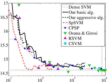
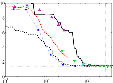
	Support Size	Support Size

	Web	TIMIT
Test error
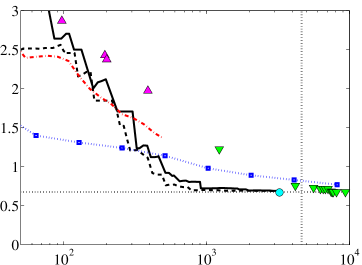
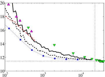
	Support Size	Support Size

	Forest
Test error
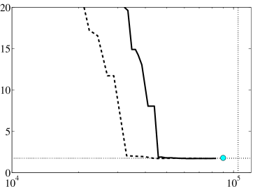
	Support Size

Figure 3.6: Plots of test error (linear scale) versus support size (log scale). The horizontal and vertical dotted lines are the test error rate and support size of the classifier found by GTSVM. TIMIT was not included in the experiments of Nguyen et al. [42]. On Forest, SpSVM ran out of memory, CPSP failed to terminate in one week for 4096 or more basis functions, LibSVM failed to optimize the SVR problem (Problem 3.8) in $4$ days for $\epsilon<1$, and RSVM’s solutions were limited to $200$ support vectors, far too few to perform well on this dataset.

Basing our experiments on recent comparisons between sparse SVM optimizers [33, 42], we compare our implementation to the following methods:

1. SpSVM [33], using Olivier Chapelle’s implementation.

2. CPSP [29], using SVM-Perf.

3. Osuna & Girosi’s algorithm [45], using LibSVM [12] to optimize the resulting SVR problems.

4. RSVM [36], using the LibSVM Tools implementation [37].

5. CSVM [42]. We did not perform these experiments ourselves, and instead present the results reported in the CSVM paper.

Our comparison was performed on the datasets listed in Table 3.5. Adult and IJCNN are the “a8a” and “ijcnn1” datasets from LibSVM Tools. Web and Forest are from the LibCVM Toolkit. We also use a multiclass dataset derived from the TIMIT speech corpus, on which we perform one-versus-rest classification, with class number $3$ (the phoneme /k/) providing the “positive” instances. Both Adult and TIMIT have relatively high error rates, making them more challenging for sparse SVM solvers. Both our algorithm and that of Osuna & Girosi require a reference classifier $w$, found using GTSVM [17].

We experimented with two versions of our algorithm, both incorporating the modifications of Section 17, differing only in whether they include the aggressive variation. For the “basic” version, we tried $\eta=\{4^{-4},4^{-3},\dots,4^{2}\}$, keeping track of the progress of the algorithm throughout the course of optimization. For each support size, we chose the best $\eta$ based on a validation set (half of the original test set) reporting errors on an independent test set (the other half). This was then averaged over $100$ random test/validation splits.

For the aggressive variant (Section 17.1), we experimented not only with multiple choices of $\eta$, but also termination thresholds $\epsilon\in\left\{2^{-4},2^{-3},\dots,1\right\}$, running until this threshold was satisfied. Optimization over the parameters was then performed using the same validation approach as for the “basic” algorithm.

In our CPSP experiments, the target numbers of basis functions were taken to be powers of two. For Osuna & Girosi’s algorithm, we took the SVR regularization parameter $\tilde{C}$ to be that of Table 3.5 (i.e. $\tilde{C}=C$), and experimented with $\epsilon\in\left\{2^{-16},2^{-15},\dots,2^{4}\right\}$. For RSVM, we tried subset ratios $\nu\in\left\{2^{-16},2^{-15},\dots,1\right\}$—however, the implementation we used was unable to find a support set of size larger than $200$, so many of the larger values of $\nu$ returned duplicate results.

The results are summarized in Figure 3.6. Our aggressive variant achieved a test error / support size tradeoff comparable to or better than the best competing algorithms, except on the Adult and TIMIT datasets, on the latter of which performance was fairly close to that of CPSP. Even the basic variant achieved very good results, often similar to or better than other, more complicated, methods. On the Adult data set, the test errors (reported) are significantly higher then the validation errors, indicating our methods are suffering from parameter overfitting due to too small a validation set (this is also true, to a lesser degree, on TIMIT). Note that SpSVM and CPSP, both of which perform very well, failed to find good solutions on the forest dataset within a reasonable timeframe, illustrating the benefits of the simplicity of our approach.

To summarize, not only does our proposed method achieve optimal theoretical guarantees (the best possible sparseness guarantee with the best known sample complexity and runtime for kernelized SVM learning), it is also computationally inexpensive, simple to implement, and performs well in practice.

Collaborators:

The work presented in this chapter was performed jointly with Shai Shalev-Shwartz and Nathan Srebro.

19   Proofs for Chapter 3

lem:svm-sparse:lower-bound

Let $R,\mathcal{L}^{*},\epsilon\geq 0$ be given, with $\mathcal{L}^{*}+\epsilon\leq\nicefrac{{1}}{{4}}$ and with $R^{2}$ being an integer. There exists a data distribution $\mathcal{D}$ and a reference vector $u$ such that $\left\lVert{u}\right\rVert=R$, $\mathcal{L}_{\mathrm{hinge}}\left(g_{u}\right)=\mathcal{L}^{*}$, and any $w$ which satisfies:

$$\mathcal{L}_{\mathrm{0/1}}\left(g_{w}\right)\leq\mathcal{L}^{*}+\epsilon$$

must necessarily be supported on at least $R^{2}/2$ vectors. Furthermore, the claim also holds for randomized classification rules that predict $1$ with probability $\psi(g_{u}(x))$ for some $\psi:\mathbb{R}\to[0,1]$.

We define $\mathcal{D}$ such that $i$ is sampled uniformly at random from the set $\left\{1,\dots,d\right\}$, with $d=R^{2}$, and the feature vector is taken to be $x=e_{i}$ (the $i$th standard unit basis vector) with corresponding label distributed according to $\mathrm{Pr}\left\{y=z\right\}=1-\mathcal{L}^{*}/2$. The value of $z\in\{\pm 1\}$ will be specified later. Choose ${u}_{i}=z$ for all $i$, so that $\left\lVert{u}\right\rVert=R$ and $\mathcal{L}_{\mathrm{hinge}}\left(g_{u}\right)=\mathcal{L}^{*}$.

Take $w$ to be a linear combination of $k<d/2=R^{2}/2$ vectors. Then $g_{w}(x)=0$ on any $x$ which is not in its support set. Suppose that whenever $g_{w}(x_{i})=0$ the algorithm predicts the label $1$ with probability $p\in[0,1]$ ($p=\psi(0)$ for a randomized classifier). If $p\geq 1/2$ we’ll set $z=-1$, and if $p<1/2$ we’ll set $z=1$. This implies that:

$$\mathcal{L}_{\mathrm{0/1}}\left(g_{w}\right)\geq\frac{d-k}{2d}>\frac{1}{4}\geq\mathcal{L}^{*}+\epsilon$$

which concludes the proof. lem:svm-sparse:slant-loss

For any $w$, and any $\tilde{w}$ for which Problem 3.1 has value $f\left(\tilde{w}\right)\leq\nicefrac{{1}}{{2}}$, we have that

$$\mathbb{E}_{Z}\left[\hat{\mathcal{L}}_{0/1}\left(\tilde{g}_{\tilde{w}}\right)\right]=\hat{\mathcal{L}}_{slant}\left(g_{\tilde{w}}\right)\leq\hat{\mathcal{L}}_{hinge}\left(g_{w}\right)$$

It remains only to establish that $\hat{\mathcal{L}}_{slant}\left(g_{\tilde{w}}\right)\leq\hat{\mathcal{L}}_{hinge}\left(g_{w}\right)$. For every $x_{i},y_{i}$, consider the following three cases:

1. If $y_{i}\left\langle{w},{\Phi(x_{i})}\right\rangle\leq 0$, then $\ell_{slant}(y_{i}g_{\tilde{w}}(x_{i}))\leq 1\leq\ell_{hinge}(y_{i}g_{w}(x_{i}))$.

2. If $0<y_{i}\left\langle{w},{\Phi(x_{i})}\right\rangle<1$, then $\ell_{slant}(y_{i}g_{\tilde{w}}(x_{i}))\leq\ell_{slant}(y_{i}g_{w}(x_{i})-\nicefrac{{1}}{{2}})\leq\ell_{hinge}(y_{i}g_{w}(x_{i}))$.

3. If $y_{i}\left\langle{w},{\Phi(x_{i})}\right\rangle\geq 1$, then $\ell_{slant}(y_{i}g_{\tilde{w}}(x_{i}))\leq\ell_{slant}(\nicefrac{{1}}{{2}})=0=\ell_{hinge}(y_{i}g_{w}(x_{i}))$.

Hence, $\ell_{slant}(y_{i}g_{\tilde{w}}(x_{i}))\leq\ell_{hinge}(y_{i}g_{w}(x_{i}))$, which completes the proof. lem:svm-sparse:convergence-rate

After $T\leq 4\left\lVert{w}\right\rVert^{2}$ iterations of subgradient descent with $\eta=\nicefrac{{1}}{{2}}$, we obtain a solution of the form $\tilde{w}=\frac{1}{2}\sum_{t=1}^{T}y_{i_{t}}\Phi(x_{i_{t}})$ which has value $f\left(\tilde{w}\right)\leq\nicefrac{{1}}{{2}}$.

First note that $f(w)\leq 0$. Relying on this possible solution $w$, the Lemma follows from standard convergence bounds of subgradient descent (see e.g. Section 1.2 of Nesterov [41]): with the step size $\eta=\epsilon$, after performing $\left\lVert{w}\right\rVert^{2}/\epsilon^{2}$ iterations, at least one iterate $\tilde{w}^{(t)}$ will have an objective function value no greater than $\epsilon$. Choosing $\epsilon=\nicefrac{{1}}{{2}}$ gives the desired result. thm:svm-sparse:compression-bound

This is Theorem 2 of Shalev-Shwartz [50]. Let $k$ and $n$ be fixed, with $n\geq 2k$, and let $A:\left(\mathbb{R}^{d}\times\left\{\pm 1\right\}\right)^{k}\rightarrow\mathcal{H}$ be a mapping which receives a list of $k$ labeled training examples, and returns a classification vector $w\in\mathcal{H}$. Use $S\in\left[n\right]^{k}$ to denote a list of $k$ training indices, and let $w_{S}$ be the result of applying $A$ to the training elements indexed by $S$. Finally, let $\ell:\mathbb{R}\rightarrow\left[0,1\right]$ be a loss function bounded below by $0$ and above by $1$, with $\mathcal{L}\left(g_{w}\right)$ and $\hat{\mathcal{L}}\left(g_{w}\right)$ the expected loss, and empirical loss on the training set, respectively. Then, with probability $1-\delta$, for all $S$:

$$\mathcal{L}\left(g_{w_{S}}\right)\leq\hat{\mathcal{L}}\left(g_{w_{S}}\right)+\sqrt{\frac{32\hat{\mathcal{L}}\left(g_{w_{S}}\right)\left(k\log n+\log\frac{1}{\delta}\right)}{n}}+\frac{8\left(k\log n+\log\frac{1}{\delta}\right)}{n}$$

Consider, for some fixed $\delta^{\prime}$, the probability that there exists a $S\subseteq\left\{1,\dots,n\right\}$ of size $k$ such that:

$$\mathcal{L}\left(g_{w_{S}}\right)\geq\hat{\mathcal{L}}_{\mbox{test}}\left(g_{w_{S}}\right)+\sqrt{\frac{2\hat{\mathcal{L}}_{\mbox{test}}\left(g_{w_{S}}\right)\log\frac{1}{\delta^{\prime}}}{\left(n-k\right)}}+\frac{4\log\frac{1}{\delta^{\prime}}}{n-k}$$

where $\hat{\mathcal{L}}_{\mbox{test}}\left(g_{w}\right)=\frac{1}{n-k}\sum_{i\notin S}\ell\left(y_{i}g_{w}\left(x_{i}\right)\right)$ is the empirical loss on the complement of $S$. It follows from Bernstein’s inequality that, for a particular $S$, the above holds with probability at most $\delta^{\prime}$. By the union bound:

$$n^{k}\delta^{\prime}\geq\mathrm{Pr}\left\{\exists S\in[n]^{k}:\mathcal{L}\left(g_{w_{S}}\right)\geq\hat{\mathcal{L}}_{\mbox{test}}\left(g_{w_{S}}\right)+\sqrt{\frac{2\hat{\mathcal{L}}_{\mbox{test}}\left(g_{w_{S}}\right)\log\frac{1}{\delta^{\prime}}}{\left(n-k\right)}}+\frac{4\log\frac{1}{\delta^{\prime}}}{n-k}\right\}$$

Let $\delta=n^{k}\delta^{\prime}$. Notice that $\left(n-k\right)\hat{\mathcal{L}}_{\mbox{test}}\left(g_{w_{S}}\right)\leq n\hat{\mathcal{L}}\left(g_{w_{S}}\right)$, so:

$$\delta\geq\mathrm{Pr}\left\{\exists S\in[n]^{k}:\mathcal{L}\left(g_{w_{S}}\right)\geq\frac{n\hat{\mathcal{L}}\left(g_{w_{S}}\right)}{n-k}+\sqrt{\frac{2n\hat{\mathcal{L}}\left(g_{w_{S}}\right)\log\frac{n^{k}}{\delta}}{\left(n-k\right)^{2}}}+\frac{4\log\frac{n^{k}}{\delta}}{n-k}\right\}$$

Because $\hat{\mathcal{L}}\left(g_{w_{S}}\right)\leq 1$ and $k\leq n$, it follows that $k\hat{\mathcal{L}}\left(g_{w_{S}}\right)\leq 2n\log n$, and therefore that $\frac{k}{n-k}\hat{\mathcal{L}}\left(g_{w_{S}}\right)\leq\sqrt{\frac{2nk\hat{\mathcal{L}}\left(g_{w_{S}}\right)\log n}{\left(n-k\right)^{2}}}\leq\sqrt{\frac{2n\hat{\mathcal{L}}\left(g_{w_{S}}\right)\log\frac{n^{k}}{\delta}}{\left(n-k\right)^{2}}}$. Hence:

$$\delta\geq\mathrm{Pr}\left\{\exists S\in[n]^{k}:\mathcal{L}\left(g_{w_{S}}\right)\geq\hat{\mathcal{L}}\left(g_{w_{S}}\right)+\sqrt{\frac{8n\hat{\mathcal{L}}\left(g_{w_{S}}\right)\log\frac{n^{k}}{\delta}}{\left(n-k\right)^{2}}}+\frac{4\log\frac{n^{k}}{\delta}}{n-k}\right\}$$

Using the assumption that $n\geq 2k$ completes the proof. lem:svm-sparse:generalization-from-compression

With probability at least $1-\delta$ over the training set, if $\tilde{w}$ is a solution with value $f(\tilde{w})\leq\nicefrac{{1}}{{2}}$ to Problem 3.1 found by performing $T=4\left\lVert{w}\right\rVert^{2}$ iterations of subgradient descent (see Algorithm 3.2 and Lemma LABEL:lem:svm-sparse:convergence-rate), then:

$$\mathcal{L}_{\mathrm{0/1}}\left(\tilde{g}_{\tilde{w}}\right)\leq\hat{\mathcal{L}}_{\mathrm{hinge}}\left(\tilde{g}_{\tilde{w}}\right)+O\left(\sqrt{\hat{\mathcal{L}}_{\mathrm{hinge}}\left(g_{w}\right)\frac{\left\lVert{w}\right\rVert^{2}\log n+\log\frac{1}{\delta}}{n}}+\frac{\left\lVert{w}\right\rVert^{2}\log n+\log\frac{1}{\delta}}{n}\right)$$

provided that $n\geq 2T$.

Because $\tilde{w}$ is found via subgradient descent,it can be written in the form $\tilde{w}=\eta\sum_{i\in S}y_{i}x_{i}=A(S)$ with $S\in\left[n\right]^{k}$, and $k=T=4\left\lVert{w}\right\rVert^{2}$. Hence, by the compression bound of Theorem LABEL:thm:svm-sparse:compression-bound, we have that with probability $1-\delta$:

$$\mathcal{L}_{\mathrm{slant}}\left(g_{\tilde{w}}\right)\leq\hat{\mathcal{L}}_{\mathrm{slant}}\left(g_{\tilde{w}}\right)+\sqrt{\frac{32\hat{\mathcal{L}}_{\mathrm{slant}}\left(g_{\tilde{w}}\right)\left(k\log n+\log\frac{1}{\delta}\right)}{n}}+\frac{8\left(k\log n+\log\frac{1}{\delta}\right)}{n}$$

The randomized classification rule $\tilde{g}_{\tilde{w}}$ was defined in such a way that $\ell_{slant}\left(yg_{\tilde{w}}\left(x\right)\right)=\mathbb{E}\left[\ell_{0/1}\left(y\tilde{g}_{\tilde{w}}\left(x\right)\right)\right]$. Furthermore, as was shown in Lemma LABEL:lem:svm-sparse:slant-loss, $\hat{\mathcal{L}}_{\mathrm{slant}}\left(g_{\tilde{w}}\right)\leq\hat{\mathcal{L}}_{\mathrm{hinge}}\left(g_{w}\right)$. Plugging these results into the above equation:

$$\mathcal{L}_{\mathrm{0/1}}\left(\tilde{g}_{\tilde{w}}\right)\leq\hat{\mathcal{L}}_{\mathrm{hinge}}\left(g_{w}\right)+\sqrt{\frac{32\hat{\mathcal{L}}_{\mathrm{hinge}}\left(g_{w}\right)\left(k\log n+\log\frac{1}{\delta}\right)}{n}}+\frac{8\left(k\log n+\log\frac{1}{\delta}\right)}{n}$$

The above holds for all $w$ such that $\tilde{w}$ is a $\nicefrac{{1}}{{2}}$-suboptimal solution to the corresponding instance of Problem 3.1. Plugging the assumption that $k=4\left\lVert{w}\right\rVert^{2}$ completes the proof. thm:svm-sparse:main-smooth

Let $R\in\mathbb{R}_{+}$ be fixed. With probability $1-\delta$ over the training sample, uniformly over all pairs $w,\tilde{w}\in\mathcal{H}$ such that $\left\lVert{w}\right\rVert\leq R$ and $\tilde{w}$ has objective function $f(\tilde{w})\leq\nicefrac{{1}}{{3}}$ in Problem 3.3:

$$\mathcal{L}_{\mathrm{0/1}}\left(\tilde{g}_{\tilde{w}}\right)\leq\hat{\mathcal{L}}_{\mathrm{hinge}}\left(g_{w}\right)$$

$$+O\left(\sqrt{\frac{\hat{\mathcal{L}}_{\mathrm{hinge}}\left(g_{w}\right)R^{2}\log^{3}n}{n}}+\sqrt{\frac{\hat{\mathcal{L}}_{\mathrm{hinge}}\left(g_{w}\right)\log\frac{1}{\delta}}{n}}+\frac{R^{2}\log^{3}n}{n}+\frac{\log\frac{1}{\delta}}{n}\right)$$

Because our bound is based on a smooth loss, we begin by defining the bounded $4$-smooth loss $\ell_{smooth}(z)$ to be $1$ if $z<-\nicefrac{{1}}{{2}}$, $0$ if $z>\nicefrac{{2}}{{3}}$, and $\nicefrac{{1}}{{2}}\left(1+\cos\left(\nicefrac{{\pi}}{{2}}\left(1+\nicefrac{{1}}{{7}}\left(12z-1\right)\right)\right)\right)$ otherwise. This function is illustrated in Figure 3.3—notice that it upper-bounds the slant-loss, and lower-bounds the hinge loss even when shifted by $\nicefrac{{1}}{{3}}$. Applying Theorem 1 of Srebro et al. [56] to this smooth loss yields that, with probability $1-\delta$, uniformly over all $\tilde{w}$ such that $\left\lVert{\tilde{w}}\right\rVert\leq R$:

$$\mathcal{L}_{\mathrm{smooth}}\left(g_{\tilde{w}}\right)\leq\hat{\mathcal{L}}_{\mathrm{smooth}}\left(g_{\tilde{w}}\right)+$$

$$O\left(\sqrt{\frac{\hat{\mathcal{L}}_{\mathrm{smooth}}\left(g_{\tilde{w}}\right)R^{2}\log^{3}n}{n}}+\sqrt{\frac{\hat{\mathcal{L}}_{\mathrm{smooth}}\left(g_{\tilde{w}}\right)\log\frac{1}{\delta}}{n}}+\frac{R^{2}\log^{3}n}{n}+\frac{\log\frac{1}{\delta}}{n}\right)$$

Just as the empirical slant-loss of a $\tilde{w}$ with $f(\tilde{w})\leq\nicefrac{{1}}{{2}}$ is upper bounded by the empirical hinge loss of $w$, the empirical smooth loss of a $\tilde{w}$ with $f(\tilde{w})\leq\nicefrac{{1}}{{3}}$ is upper-bounded by the same quantity. As was argued in the proof of Lemma LABEL:lem:svm-sparse:slant-loss, this follows directly from Problem 3.3, and the definition of the smooth loss. Combining this with the facts that the slant-loss lower bounds the smooth loss, and that $\mathcal{L}_{\mathrm{slant}}\left(g_{\tilde{w}}\right)=\mathcal{L}_{\mathrm{0/1}}\left(\tilde{g}_{\tilde{w}}\right)$, completes the proof. thm:svm-sparse:main-compression

For an arbitrary (unknown) reference classifier $u$, with probability at least $1-2\delta$ over a training set of size:

$$n=\tilde{O}\left(\left(\frac{\mathcal{L}_{\mathrm{hinge}}\left(g_{u}\right)+\epsilon}{\epsilon}\right)\frac{\left\lVert{u}\right\rVert^{2}}{\epsilon}\log\frac{1}{\delta}\right)$$

the procedure above finds a predictor $\tilde{w}$ supported on at most $O(\left\lVert{u}\right\rVert^{2})$ training vectors and error $\mathcal{L}_{\mathrm{0/1}}\left(\tilde{g}_{\tilde{w}}\right)\leq\mathcal{L}_{\mathrm{hinge}}\left(g_{u}\right)+O(\epsilon)$

First, note that with the specified sample size, applying Bernstein’s inequality to the fixed predictor $u$, we have that with probability at least $1-\delta$,

$$\hat{\mathcal{L}}_{\mathrm{hinge}}\left(u\right)\leq\mathcal{L}_{\mathrm{hinge}}\left(u\right)+\epsilon.$$ (3.9)

Combining Equation 3.9 with the SVM training goal (Step 1) and Lemma LABEL:lem:svm-sparse:slant-loss, we have that $\hat{\mathcal{L}}_{\mathrm{slant}}\left(g_{\tilde{w}}\right)\leq\mathcal{L}_{\mathrm{hinge}}\left(g_{u}\right)+O(\epsilon)$. Following Lemma LABEL:lem:svm-sparse:convergence-rate we can apply Lemma LABEL:lem:svm-sparse:generalization-from-compression with $T=O(\|u\|^{2})$, and plugging in the specified sample complexity, we have $\mathcal{L}_{\mathrm{slant}}\left(g_{\tilde{w}}\right)\leq\hat{\mathcal{L}}_{\mathrm{slant}}\left(g_{\tilde{w}}\right)$. Combining the two inequalities, and recalling that the slant-loss of $g_{\tilde{w}}$ is the same as the expected $0/1$ error of $\tilde{g}_{\tilde{w}}$, we obtain $\mathcal{L}_{\mathrm{0/1}}\left(\tilde{g}_{\tilde{w}}\right)\leq\mathcal{L}_{\mathrm{hinge}}\left(g_{u}\right)+O(\epsilon)$. Lemma LABEL:lem:svm-sparse:convergence-rate also establishes the desired bound on the number of support vectors.

Part II   Principal Component Analysis

Basic Algorithms

20   Overview

Principal Component Analysis (PCA) is a ubiquitous tool used in many data analysis, machine learning and information retrieval applications. It is used for obtaining a lower dimensional representation of a high dimensional signal that still captures as much as possible of the original signal. Such a low dimensional representation can be useful for reducing storage and computational costs, as complexity control in learning systems, or to aid in visualization.

Uncentered PCA is typically phrased as a question about a fixed dataset: given $n$ vectors in $\mathbb{R}^{d}$, what is the $k$-dimensional subspace that captures most of the variance in the dataset? (or equivalently, that is best in reconstructing the vectors, minimizing the sum squared distances, or residuals, to the subspace). It is well known that this subspace is given by the leading $k$ components of the singular value decomposition of the data matrix (or equivalently the top $k$ eigenvectors of the empirical second moment matrix). And so, the study of computational approaches for PCA has mostly focused on methods for finding the SVD (or leading components of the SVD) of a given $n\times d$ matrix.

Our treatment of this problem departs from the traditional statistical approach in that we view PCA as a stochastic optimization problem, where the goal is to optimize a “population objective” based on i.i.d. draws from the population. That is, we have some unknown source (“population”) distribution $\mathcal{D}$ over $\mathbb{R}^{d}$, and the goal is to find the $k$-dimensional subspace maximizing the (uncentered) variance of $\mathcal{D}$ inside the subspace (or equivalently, minimizing the average squared residual in the population), based on i.i.d. samples from $\mathcal{D}$. The main point here is that the true objective does not measure how well the subspace captures the sample (i.e. the “training error”), but rather how well the subspace captures the underlying source distribution (i.e. the “generalization error”). Furthermore, we are not concerned here with capturing some “true” subspace (in which case one might quantify success as e.g. the “angle” between the found subspace and the “true” subspace), but rather at finding a “good” subspace, which has a near-optimal value of the PCA objective. This will be formalized more in Section 21.

The straightforward approach is “Sample Average Approximation” (SAA) (i.e. “Empirical Risk Minimization”), in which one collects a sample of data points, and then optimizes an empirical version of the objective on the sample using standard deterministic techniques (in this case linear algebra). In the case of uncentered PCA, this amounts to computing the empirical second-moment matrix of the sample, and then seeking the best rank-$k$ approximation to it, e.g. by computing the leading components of its eigendecomposition. The success of this approach is measured not by how well we approximate the empirical second-moment matrix, but rather how well the subspace we obtain captures the unknown source distribution (i.e. the population second-moment matrix). This approach will be considered in greater detail in Section 22.

The alternative, which we advocate here, is a “Stochastic Approximation” (SA) approach. A SA algorithm is iterative—in each iteration a single sampled point is used to perform an update, as in Stochastic Gradient Descent (SGD, the canonical stochastic approximation algorithm). In the context of PCA, one iteratively uses vectors sampled from $\mathcal{D}$ to update the subspace being considered.

Stochastic approximation has been shown to be computationally preferable to statistical average approximation (i.e. to “batch” methods) both theoretically and empirically for learning [5, 51] and more broadly for stochastic optimization [39]. Accordingly, SA approaches, mostly variants of SGD, are often the methods of choice for many learning problems, especially when very large datasets are available [53, 14, 55].

This chapter will begin, in Section 21, with a description of two equivalent versions of the PCA objective: one of which represents the underlying PCA subspace as a set of vectors spanning it, represented as the orthonormal columns of a rectangular matrix $U$; the other as a projection matrix $M$ which projects onto the PCA subspace. We call these the $U$-based and $M$-based objectives, respectively. Section 22 will discuss the SAA approach, while, in Section 23, we will present the “stochastic power method”, a catch-all algorithm of which many variants may be found in literature dating back several decades, and highlight its relationship to the well-known power method for finding the maximum eigenvectors of a matrix. In Section 24, an “incremental algorithm” will be discussed. Both of the latter two algorithms have been found to work well in practice, but suffer from serious theoretical limitations—the former is known to converge with probability one, but the rate of convergence is unknown, while the latter fails to converge entirely on certain problem instances. Portions of this chapter, in particular Sections 23 and 24, were originally presented at the 50th Allerton Conference on Communication, Control and Computing [1].

These basic algorithms form the foundation for Chapters 5 and 6, which discuss theoretically justified and analyzable algorithms for solving PCA problems, the first originally due to Warmuth and Kuzmin [60], and the second novel.

21   Objective

	Description
$\mathcal{D}$	Data distribution such that $\left\lVert{x}\right\rVert\leq 1$ for $x\sim\mathcal{D}$
$n,T\in\mathbb{N}$	Training size ($n$ for a “batch” algorithm, $T$ for a stochastic algorithm)
$d\in\mathbb{N}$	Data dimension
$k\in\mathbb{N}$	PCA subspace dimension
$x_{1},\dots,x_{n}\in\mathbb{R}^{d}$	Training samples
$U\in\mathbb{R}^{n\times d}$	PCA solution (columns span the maximal space)
$M\in\mathbb{R}^{n\times n}$	PCA solution (projection matrix onto the maximal space, or “relaxed” projection matrices in Chapter 6)
$W\in\mathbb{R}^{n\times n}$	PCA solution (“relaxed” projection matrix onto the minimal space in Chapter 5)
$k_{t}^{\prime}\in\mathbb{N}$	Number of nontrivial eigenvalues of the $t$th iterate found by the algorithms of Chapters 5 and 6
$K\in\mathbb{N}$	Upper bound on the rank of the iterates found by the capped MSG algorithm of Chapter 6

Table 4.1: Summary of common notation across Chapters 4, 5 and 6. In the two latter chapters, $M$ will be relaxed to not be a projection matrix onto the PCA space, but rather a (potentially full-rank) PSD matrix for which the magnitude of each eigenvalue represents the likelihood that the corresponding eigenvector is one of the principal components.

The goal of uncentered PCA is to find, for a distribution $\mathcal{D}$ over vectors $x\in\mathbb{R}^{d}$, the subspace of dimension $k$ for which the projections of $x$ onto this subspace have maximal uncentered second sample moments. To simplify the presentation, we will assume, in this chapter as well as Chapters 5 and 6, that $\left\lVert{x}\right\rVert\leq 1$ with probability $1$ for $x\sim\mathcal{D}$—this is a relatively weak assumption, since any bounded data distribution can be adjusted to satisfy it through scaling. There are a number of alternative perspectives which one can take, which ultimately lead to the same problem formulation. For example, one may wish to find a lower-dimensional representation of the data which minimizes the $L^{2}$ reconstruction error:

$$\underset{U^{T}U=I}{\operatorname{argmin}}\mathbb{E}_{x\sim\mathcal{D}}\left[\left\lVert{x-UU^{T}x}\right\rVert_{2}^{2}\right]$$

where $U\in\mathbb{R}^{d\times k}$ has orthonormal columns, which, at the optimum, will be the $k$ maximal eigenvectors of the second moment matrix $\Sigma=\mathbb{E}_{x\sim\mathcal{D}}\left[xx^{T}\right]$. Alternatively, perhaps one wishes to find the projection $UU^{T}$ of $\Sigma$ onto a $k$-dimensional subspace such that the result is closest to $\Sigma$ in terms of the trace norm:

$$\underset{U^{T}U=I}{\operatorname{argmin}}\operatorname{tr}\left(U^{T}\Sigma U-\Sigma\right)$$

Both of these examples may be simplified to the problem of finding a $U$ satisfying:

$$\underset{U^{T}U=I}{\operatorname{argmin}}\mathbb{E}_{x\sim\mathcal{D}}\left[x^{T}UU^{T}x\right]$$

The orthonormality constraint on the columns of $U$ may be weakened to the constraint that all eigenvalues of $U^{T}U$ must be at most one, because if any eigenvalue of this matrix is less than one, then increasing it (in the same basis) will only increase the above objective function. Hence, for the optimal $U^{*}$, all of the eigenvalues of $\left(U^{*}\right)^{T}U^{*}$ will be $1$, implying that $\left(U^{*}\right)^{T}U^{*}=I$, and therefore that the columns of $U$ are orthonormal. This allows us to state the PCA objective in the language of optimization, as:

$$\mbox{maximize}: \mathbb{E}_{x\sim\mathcal{D}}\left[x^{T}UU^{T}x\right]$$ (4.1)

$$\mbox{subject to}: U\in\mathbb{R}^{d\times k},U^{T}U\preceq 1$$

Some of the algorithms which we will consider work not by optimizing $U$, but instead by changing the optimization variables in such as way as to optimize over a rank-$k$ positive semidefinite matrix $M\in\mathbb{R}^{d\times d}$, which we can think of as satisfying $M=UU^{T}$, giving the objective:

$$\mbox{maximize}: \mathbb{E}_{x\sim\mathcal{D}}\left[x^{T}Mx\right]$$ (4.2)

$$\mbox{subject to}: M\in\mathbb{R}^{d\times d},\sigma_{i}\left({M}\right)\in\left\{0,1\right\},\operatorname{rank}M=k$$

Here, $\sigma_{i}\left({M}\right)$ is the $i$th eigenvalue of $M$, so the constraint on the eigenvalues, combined with the rank constraint, forces $M$ to have exactly $k$ eigenvalues equal to $1$, and $n-k$ equal to $0$—in other words, $M$ is a rank-$k$ projection matrix.

Problems 4.1 and 4.2 are both stochastic, in that their objective functions are expectations over the distribution $\mathcal{D}$. In the situation we consider, and which we argue is typical in practice, we do not have direct knowledge of the distribution $\mathcal{D}$, and so cannot exactly calculate the (population) objective, let alone optimize it. Instead, we only have access to i.i.d. samples from $\mathcal{D}$—these can be thought of as “training examples”. The regime we are mostly concerned with is that in which we have an essentially unlimited supply of training examples, and would like to obtain an $\epsilon$-suboptimal solution in the least possible runtime. That is, one can think of access to an “example oracle” that generates an example on-demand, at the cost of reading the sample. We refer to such a regime, where data is abundant and the resources of interest are runtime and perhaps memory consumption, as the “data laden” regime.

The algorithms which we consider are all iterative, in that they consider training examples $x_{t}$ one-at-a-time. At every step, an estimate $U^{(t)}$ or $M^{(t)}$ is produced based on some internal state of the algorithm, a new example is obtained, and a loss is incurred in terms of the component of the example not explained by the current iterate. This loss (residual) is then used to update the internal state of the algorithm.

Problem 4.1 is a quadratic objective subject to quadratic constraints, but because it is a maximization problem, it is not a convex optimization problem. Likewise, Problem 4.2 is a linear objective subject to non-convex constraints. As a result, we may not immediately appeal to the vast literature on convex optimization to efficiently optimize either of these objectives.

The fact that the optimization problems corresponding to PCA are not convex is a major complication in designing and studying stochastic approximation methods for PCA. The empirical optimization problem is still tractable due to algebraic symmetry, and the eigendecomposition can be computed either through algebraic elimination, or through iterative local search methods such as the power method. However standard methods and analyses for stochastic convex optimization are not immediately applicable. This non-convex-but-tractable situation poses a special challenge, and we are not aware of other similar situations where stochastic optimization has been studied. Rather, in most learning applications of stochastic optimization, either stochastic gradient descent, stochastic mirror descent, or variants thereof are directly applicable, or global optimality cannot be ensured even for the deterministic empirical optimization problem (e.g. when using stochastic approximation to train deep networks).

One method for addressing this difficulty is to essentially ignore it, and use standard optimization algorithms (e.g. stochastic gradient ascent), while attempting to prove whatever bounds can be found. In Section 23, we will see an algorithm which takes this approach. Alternatively, one may continue manipulating this objective until one finds an equivalent relaxed convex optimization problem, which may then be optimized efficiently using conventional techniques. Chapters 5 and 6 will give examples of this approach.

22   Sample Average Approximation (SAA)

	Computation	Memory	Convergence
SAA	$nd^{2}$	$d^{2}$	$\sqrt{\frac{k}{n}}$
SAA (Coppersmith-Winograd)	$nd^{1.3727}$	$d^{2}$	$\sqrt{\frac{k}{n}}$
Stochastic Power Method	$Tkd$	$kd$	w.p. $1$
Incremental	$Tk^{2}d$	$kd$	no

Table 4.2: Summary of results from Sections 22, 23 and 24. All bounds are given up to constant factors. The “Convergence” column contains bounds on the suboptimality of the solution—i.e. the difference between the total variance captured by the rank-$k$ subspace found by the algorithm, and the best rank-$k$ subspace with respect to the data distribution $\mathcal{D}$. The stochastic power method converges with probability $1$, but at an unknown rate, while there exist data distributions for which the incremental algorithm fails to converge entirely. The “Coppersmith-Winograd” variant of SAA uses an asymptotically fast matrix multiplication algorithm [16] to calculate the empirical second moment matrix, and is unlikely to be useful in practical applications.

In Section 20, we mentioned the Sample Average Approximation algorithm, which is nothing more than the “traditional” technique for solving stochastic PCA problems: draw $n$ samples from $\mathcal{D}$, calculate their empirical second moment matrix, and find its eigendecomposition to derive the top-$k$ eigenvectors.

Because we’re working in the stochastic setting, this is not, as may at first be assumed, an exact solution—we want to capture most of the variance in the true second moment matrix $\Sigma$ in a $k$-dimensional subspace, while SAA gives us only the maximal subspace based on an empirical second moment matrix $\hat{\Sigma}$. The quality of its solution depends on how accurately $\hat{\Sigma}$ approximates the unknown ground truth $\Sigma$, which depends on the number of samples upon which $\hat{\Sigma}$ is based. One can derive just such a bound with a Rademacher complexity based analysis [3]:

lem:pca-introduction:saa-bound Suppose that $U\in\mathbb{R}^{d\times k}$ has orthonormal columns spanning the maximal subspace of an empirical covariance matrix $\hat{\Sigma}=(1/n)\sum_{i=1}^{n}x_{i}x_{i}^{T}$ over $n$ samples drawn i.i.d. from $\mathcal{D}$. Likewise, let $U^{*}$ be the corresponding matrix with $k$ orthogonal columns spanning the maximal subspace of the true covariance $\Sigma=\mathbb{E}_{x\sim\mathcal{D}}\left[xx^{T}\right]$. Then, with probability $1-\delta$:

$$\operatorname{tr}\left(U^{*}\right)^{T}\Sigma U^{*}-\operatorname{tr}U^{T}\Sigma U\leq O\left(\sqrt{\frac{k\log\frac{1}{\delta}}{n}}\right)$$

Observe that, while Lemma 4.7 holds uniformly for all $U$, we are now considering only a particular $U$, albeit a random variable depending on the sample (hence the need for a uniform bound). Because $U$ is the empirical optimum, it follows that $\operatorname{tr}\left(I-UU^{T}\right)\hat{\Sigma}\leq\operatorname{tr}\left(I-U^{*}\left(U^{*}\right)^{T}\right)\hat{\Sigma}$. Combining this fact with Lemmas 4.7 and 4.8 yields that, with probability $1-\delta$:

$$\operatorname{tr}\left(I-UU^{T}\right)\Sigma-\operatorname{tr}\left(I-U^{*}\left(U^{*}\right)^{T}\right)\hat{\Sigma}\leq\sqrt{\frac{k}{n}}+\sqrt{\frac{8\log\frac{2}{\delta}}{n}}$$

To complete the proof, we need only prove a bound on the difference between $\operatorname{tr}\left(I-U^{*}\left(U^{*}\right)^{T}\right)\hat{\Sigma}$ and $\operatorname{tr}\left(I-U^{*}\left(U^{*}\right)^{T}\right)\Sigma$. By Hoeffding’s inequality:

$$\mathrm{Pr}\left\{\operatorname{tr}\left(I-U^{*}\left(U^{*}\right)^{T}\right)\left(\hat{\Sigma}-\Sigma\right)\geq\epsilon\right\}\leq\exp\left(-\frac{n\epsilon}{2}\right)$$

Setting the RHS to $\delta$ and solving for $\epsilon$ yields that:

$$\epsilon=\frac{2\log\frac{1}{\delta}}{n}$$

Hence, with probability $1-2\delta$:

$$\operatorname{tr}\left(I-UU^{T}\right)\Sigma-\operatorname{tr}\left(I-U^{*}\left(U^{*}\right)^{T}\right)\Sigma\leq\sqrt{\frac{k}{n}}+\sqrt{\frac{2\log\frac{1}{\delta}}{n}}+\sqrt{\frac{8\log\frac{2}{\delta}}{n}}$$

Canceling the two $\operatorname{tr}\Sigma$ terms on the LHS, negating the inequality and simplifying yields the claimed result.

This bound tells only part of the story, since the computational cost of the SAA procedure is so high. Merely calculating the empirical second moment matrix, to say nothing of finding its eigendecomposition, costs $O(nd^{2})$ operations for a naïve implementation, $O\left(nd^{\log_{2}7-1}\right)$ using Strassen’s algorithm [62, 59] to multiply the matrix of samples with its transpose (thereby calculating $\hat{\Sigma}$), or $O\left(nd^{1.3727}\right)$ using Coppersmith and Winograd [16], the fastest-known matrix multiplication algorithm [62]. Both of the latter two algorithms (particularly the second) are widely-regarded as impractical except in highly specialized circumstances, so we will treat the computational cost as $O(nd^{2})$. The memory requirements of this algorithm are also relatively high: $d^{2}$ to store $\hat{\Sigma}$. As we will see in Chapters 5 and 6, there are stochastic algorithms which have similar sample complexity bounds to that of Lemma LABEL:lem:pca-introduction:saa-bound, and a lower computational cost. Even in this chapter, we will consider algorithms which are much “cheaper”, in that they perform less work-per-sample, and work very well in practice, although there are no known bounds on their rate of convergence.

23   The Stochastic Power Method

For convex optimization problems, stochastic gradient descent is a simple and often highly efficient optimization technique. As was previously mentioned, the $U$-optimizing PCA objective function of Problem 4.1 is convex, as is the constraint, but as the goal is maximization of this objective, the formulation of Equation 4.1 is not convex as an optimization problem. However, stochastic gradient descent is still a viable algorithm.

23.1   The Power Method

If $\Sigma=\mathbb{E}_{x\sim\mathcal{D}}\left[xx^{T}\right]$ were known exactly, then the gradient of the PCA objective function $\mathbb{E}_{x\sim\mathcal{D}}\left[x^{T}UU^{T}x\right]=\operatorname{tr}(U^{T}\Sigma U)$ with respect to $U$ would be $2\Sigma U$, leading one to consider updates of the form:

$$U^{(t+1)}=\mathcal{P}_{\textrm{orth}}\left(U^{(t)}+\eta\Sigma U^{(t)}\right)$$ (4.3)

where $\mathcal{P}_{\textrm{orth}}\left(U\right)$ performs a projection with respect to the spectral norm of $UU^{T}$ onto the set of $d\times d$ matrices with $k$ eigenvalues equal to $1$ and the rest $0$ (calling this a “projection” is a slight abuse of terminology, since it is $UU^{T}$ which is projected, not $U$ itself).

One advantage which we have in the non-stochastic setting (i.e. when $\Sigma$ is known) is that we may analytically determine the optimal value of the step size $\eta$. To this end, let’s consider only the one-dimensional case (i.e. $U$ is a column vector $u$). With this simplification in place, projection onto the constraint of Problem 4.1 can be accomplished through normalization, giving the equivalent problem:

$$\mbox{maximize}:\frac{u^{T}\Sigma u}{u^{T}u}$$ (4.4)

Because this objective function is invariant to the scale of $U$, we may, for reasons which will become clear shortly, rewrite the update of Equation 4.3 with the step size $\eta$ applied to the first term, instead of the second:

$$u^{(t+1)}=\eta u^{(t)}+\Sigma u^{(t)}$$ (4.5)

Notice that we have removed the projection step, since this is now handled as a part of the objective function. Assume without loss of generality that $\Sigma=\operatorname{diag}\left(\sigma_{1},\sigma_{2},\dots,\sigma_{d}\right)$ is diagonal. Substituting Equation 4.5 into Equation 4.4 and maximizing over $\eta$ will give the optimal step size:

$$\mbox{maximize}:\frac{\sum_{i=1}^{d}u_{i}^{2}\sigma_{i}\left(\eta+\sigma_{i}\right)^{2}}{\sum_{i=1}^{d}u_{i}^{2}\left(\eta+\sigma_{i}\right)^{2}}$$

Differentiating with respect to $\eta$:

$$\frac{\partial}{\partial\eta}= 2\frac{\sum_{i=1}^{d}u_{i}^{2}\sigma_{i}\left(\eta+\sigma_{i}\right)}{\sum_{i=1}^{d}u_{i}^{2}\left(\eta+\sigma_{i}\right)^{2}}-2\frac{\left(\sum_{i=1}^{d}u_{i}^{2}\sigma_{i}\left(\eta+\sigma_{i}\right)^{2}\right)\left(\sum_{i=1}^{d}u_{i}^{2}\left(\eta+\sigma_{i}\right)\right)}{\left(\sum_{i=1}^{d}u_{i}^{2}\left(\eta+\sigma_{i}\right)^{2}\right)^{2}}$$

$$= -2\frac{\sum_{i=1}^{d}\sum_{j=1}^{d}u_{i}^{2}u_{j}^{2}\sigma_{i}\left(\eta+\sigma_{i}\right)\left(\eta+\sigma_{j}\right)\left(\sigma_{i}-\sigma_{j}\right)}{\left(\sum_{i=1}^{d}u_{i}^{2}\left(\eta+\sigma_{i}\right)^{2}\right)^{2}}$$

$$= -2\frac{\sum_{i=1}^{d}\sum_{j=1}^{i-1}u_{i}^{2}u_{j}^{2}\left(\eta+\sigma_{i}\right)\left(\eta+\sigma_{j}\right)\left(\sigma_{i}-\sigma_{j}\right)^{2}}{\left(\sum_{i=1}^{d}u_{i}^{2}\left(\eta+\sigma_{i}\right)^{2}\right)^{2}}$$

Since this derivative is always negative for $\eta\geq 0$ (note that it will be positive for some negative choices of $\eta$, depending on the spectrum of $\Sigma$), we see that $\eta=0$ is the optimal nonnegative choice for the learning rate, yielding the widely-used power method [23]:

$$u^{(t+1)}=\Sigma u^{(t)}$$

This shows that the power method can be viewed as an instance of the gradient ascent algorithm with an exact line search. For this reason, we refer to stochastic gradient ascent on Problem 4.1 as the “stochastic power method”.

23.2   Stochastic Gradient Ascent

Since $2xx^{T}U$ is equal in expectation to $2\Sigma U$, which is the gradient of the objective of Problem 4.1, we may perform stochastic gradient ascent by iteratively sampling $x_{t}\sim\mathcal{D}$ at the $t$th iteration, and performing the following update:

$$U^{(t+1)}=\mathcal{P}_{\textrm{orth}}\left(U^{(t)}+\eta_{t}x_{t}x_{t}^{T}U^{(t)}\right)$$ (4.6)

This is the “stochastic power method”. Notice that finding $xx^{T}U$ requires only $O(kd)$ operations (two matrix-vector multiplies). The renormalization step represented by $\mathcal{P}_{\textrm{orth}}$ can be performed in $O(k^{2}d)$ operations using, e.g., the Gram-Schmidt procedure. However, it turns out that it is not necessary to renormalize, except for numerical reasons. To see this, suppose that we do renormalize $U^{(t)}$ after each iteration. We may then write $U^{(t)}=Q^{(t)}R^{(t)}$ with $Q^{(t)}$ having orthonormal columns and $R^{(t)}$ being a nonsingular $k\times k$ matrix (this is not necessarily a QR factorization, although it may be, if one renormalizes using Gram-Schmidt). The matrix $Q^{(t)}$ is then the renormalized version of $U^{(t)}$. With this representation of renormalization, the $1$-step SGD update of Equation 4.6 is:

$$U^{(t+1)}= Q^{(t)}+\eta_{t}x_{t}x_{t}^{T}Q^{(t)},$$

$$U^{(t+1)}R^{(t)}= U^{(t)}+\eta_{t}x_{t}x_{t}^{T}U^{(t)}$$

From this equation, it is easy to prove by induction on $t$ that if $V^{(t)}$ is the sequence of iterates which would result if renormalization was not performed, then $V^{(t)}=Q^{(t)}R^{(t)}R^{(t-1)}\cdots R^{(1)}$. Because $R^{(t)}R^{(t-1)}\cdots R^{(1)}$ is a product of nonsingular matrices, it is nonsingular, showing that $V^{(t)}$ and $Q^{(t)}$ span the same subspace.

As a result of this observation, renormalization may be performed for purely numerical reasons, and only very infrequently. Hence, the computational cost of renormalization may be ignored, showing that performing $T$ iterations of SGD costs only $O(Tkd)$ operations and $O\left(kd\right)$ memory (to store $U$), both of which are better by a factor of $d/k$ than the cost of “naïve” SAA (see Section 22), if $T=n$. For small $k$ and large $d$, this represents an enormous potential performance difference over non-stochastic linear algebra-based methods.

Although not presented as instances of SGD, there are a number of algorithms in the literature that perform precisely the above SGD update, differing only in how they renormalize. For example, Oja and Karhunen [44] perform Gram-Schmidt orthonormalization after every iteration, while the popular generalized Hebbian algorithm [48], which was later generalized to the kernel PCA setting by Kim et al. [34], performs a partial renormalization. Both of these algorithms converge with probability $1$ (under certain conditions on the distribution $\mathcal{D}$ and step sizes $\eta_{t}$). However, the rate of convergence is not known.

24   The Incremental Algorithm

One of the most straightforward ways to perform PCA on the $M$-based objective of Problem 4.2 is empirical risk minimization (ERM): at every step $t$, take $C^{(t)}=\frac{1}{t}\sum_{s=1}^{t}x_{s}x_{s}^{T}$ to be the empirical second-moment matrix of all of the samples seen so far, calculate its eigendecomposition, compute the top $k$ eigenvectors, say $U^{(t)}$, of $C^{(t)}$ and take $M^{(t)}=U^{(t)}\left(U^{(t)}\right)^{T}$.

Despite being perfectly sensible, this is far from being a practical solution. Calculating $C^{(t+1)}$ from $C^{(t)}$ requires $O(d^{2})$ operations, to say nothing of then finding its eigendecomposition—this algorithm is simply far too expensive. One can, however, perform approximate ERM at a much lower computational cost by explicitly constraining the rank of the second-moment estimates $C^{(t)}$, and updating these estimates incrementally, as each new sample is observed [1]. Rather than defining $(t+1)C^{(t+1)}=tC^{(t)}+x_{t}x_{t}^{T}$, one instead takes:

$$(t+1)\tilde{C}^{(t+1)}=\mathcal{P}_{\textrm{rank-$k$}}\left(t\tilde{C}^{(t)}+x_{t}x_{t}^{T}\right)$$

where $\mathcal{P}_{\textrm{rank-$k$}}\left(\cdot\right)$ projects its argument onto the set of rank-$k$ matrices with respect to the Frobenius norm (i.e. sets all but the top $k$ eigenvalues to zero).

$\mbox{{rank1-update}}\left(d,k^{\prime}:\mathbb{N},U:\mathbb{R}^{d\times k^{\prime}},\sigma:\mathbb{R}^{k^{\prime}},\eta\in\mathbb{R},x:\mathbb{R}^{d}\right)$
1	$\hat{x}\leftarrow U^{T}x$; $x_{\perp}\leftarrow x-U\hat{x}$; $r\leftarrow\left\lVert{x_{\perp}}\right\rVert$;
2	$\mbox{{if }}r>0$
3		$V^{\prime},\sigma^{\prime}\leftarrow\mbox{{eig}}([\mbox{{diag}}(\sigma)+\eta\hat{x}\hat{x}^{T},\eta r\hat{x};\eta r\hat{x}^{T},\eta r^{2}])$;
4		$U^{\prime}\leftarrow[U,x_{\perp}/r]V^{\prime}$;
5	else
6		$V^{\prime},\sigma^{\prime}\leftarrow\mbox{{eig}}(\mbox{{diag}}(\sigma)+\eta\hat{x}\hat{x}^{T})$;
7		$U^{\prime}\leftarrow UV^{\prime}$;
8	$\mbox{{return }}U^{\prime},\sigma^{\prime}$;

Algorithm 4.3 Routine which computes an eigendecomposition of $M+\eta xx^{T}$ from a rank-$k^{\prime}$ eigendecomposition $M=U\mbox{{diag}}(\sigma)U^{T}$. The computational cost of this algorithm is dominated by the matrix multiplication defining $U^{\prime}$ (line $4$ or $7$) costing $O((k^{\prime})^{2}d)$ operations.

This update can be performed efficiently by maintaining an up-to-date eigendecomposition of $\tilde{C}^{(t)}$ which is updated at every iteration. Take $t\tilde{C}^{(t)}=U\mbox{{diag}}(\sigma)U^{T}$ to be an eigendecomposition of $t\tilde{C}^{(t)}$, where $U\in\mathbb{R}^{d\times k^{\prime}}$ has orthonormal columns, and the rank $k^{\prime}$ of $\tilde{C}^{(t)}$ satisfies $k^{\prime}\leq k$. In order to find an eigendecomposition of $t\tilde{C}^{(t)}+x_{t}x_{t}^{T}$, we will consider the component of $x_{t}$ which lies in the span of the columns of $U$ separately from the orthogonal component $x_{\perp}=(I-U)(I-U)^{T}x_{t}$ with norm $r=\left\lVert{x_{\perp}}\right\rVert$. This gives that, if $r>0$ (the $r=0$ case is trivial):

$$tC^{(t)}+x_{t}x_{t}^{T}=\left[\begin{array}[]{cc}U&\frac{x_{\perp}}{r}\end{array}\right]\left[\begin{array}[]{cc}\mbox{diag}(\sigma)+U^{T}x_{t}x_{t}^{T}U&rUU^{T}x_{t}\\ rx_{t}^{T}UU^{T}&1\end{array}\right]\left[\begin{array}[]{cc}U&\frac{x_{\perp}}{r}\end{array}\right]^{T}$$

Taking the eigendecomposition of the rank-$k^{\prime}+1$ matrix in the above expression:

$$\left[\begin{array}[]{cc}\mbox{diag}(\sigma)+U^{T}x_{t}x_{t}^{T}U&rUU^{T}x_{t}\\ rx_{t}^{T}UU^{T}&1\end{array}\right]=V^{\prime}\mbox{diag}\left(\sigma^{\prime}\right)\left(V^{\prime}\right)^{T}$$

gives that:

$$tC^{(t)}+x_{t}x_{t}^{T}= \left(\left[\begin{array}[]{cc}U&\frac{x_{\perp}}{r}\end{array}\right]V^{\prime}\right)\mbox{diag}\left(\sigma^{\prime}\right)\left(\left[\begin{array}[]{cc}U&\frac{x_{\perp}}{r}\end{array}\right]V^{\prime}\right)^{T}$$

Hence, the new vector of nonzero eigenvalues is $\sigma^{\prime}$, with the corresponding eigenvectors being:

$$U^{\prime}=\left[\begin{array}[]{cc}U&\frac{x_{\perp}}{r}\end{array}\right]V^{\prime}$$

Algorithm 4.3 contains pseudocode which implements this operation, and will find an eigendecomposition of $t\tilde{C}^{(t)}+x_{t}x_{t}^{T}$ of rank at most $k^{\prime}+1$, as $U^{\prime},\sigma^{\prime}=\mbox{{rank1-update}}(d,k^{\prime},U,\sigma,1,x_{t})$ (this algorithm takes an additional parameter $\eta$ which will not be needed until Chapter 6). Projecting onto the set of rank $k$ matrices amounts to removing all but the top $k$ elements of $\sigma^{\prime}$, along with the corresponding columns of $U^{\prime}$. The next iterate then satisfies $t\tilde{C}^{(t+1)}=U^{\prime}\mbox{{diag}}(\sigma^{\prime})\left(U^{\prime}\right)^{T}$. The total computational cost of performing this update $O((k^{\prime})^{2}d)\leq O(k^{2}d)$ operations, which is superior to the $d^{2}$ computational cost of “true” ERM, since for most applications there would be little point in performing PCA unless $k\ll d$. The memory usage is, likewise, better than that of SAA, since the dominant storage requirement is that of the matrix $U$, which contains $kd$ elements.

In Arora et al. [1], we found that this “incremental algorithm” performs extremely well on real datasets—it was the best, in fact, among the compared algorithms. However, there exist somewhat-contrived cases in which this algorithm entirely fails to converge. For example, If the data are drawn from a discrete distribution $\mathcal{D}$ which samples $[\sqrt{3},0]^{T}$ with probability $1/3$ and $[0,\sqrt{2}]^{T}$ with probability $2/3$, and one runs the incremental algorithm with $k=1$, then it will converge to $[1,0]^{T}$ with probability $5/9$, despite the fact that the maximal eigenvector is $[0,1]^{T}$. The reason for this failure is essentially that the orthogonality of the data interacts poorly with the low-rank projection: any update which does not entirely displace the maximal eigenvector in one iteration will be removed entirely by the projection, causing the algorithm to fail to make progress.

The incremental algorithm is of interest only because of its excellent empirical performance. In Chapter 6, we will develop a similar algorithm which is more theoretically justified, less likely to fail, and still performs well in practice.

Collaborators:

The novel content of this chapter (particularly Section 24) was performed jointly with Raman Arora, Karen Livescu and Nathan Srebro.

25   Proof of Lemma LABEL:lem:pca-introduction:saa-bound

Our proof of Lemma LABEL:lem:pca-introduction:saa-bound will follow a similar outline to the proof of Lemma LABEL:lem:svm-introduction:generalization-from-expected-loss in Chapter 1. The first step is to determine the how many samples we must draw in order to ensure that, uniformly over all $U\in\mathbb{R}^{d\times k}$ with orthonormal columns, the expected loss suffered by $U$ is close to the empirical loss:

Lemma 4.7.

Define $\hat{\Sigma}=(1/n)\sum_{i=1}^{n}x_{i}x_{i}^{T}$ to be the empirical covariance matrix over $n$ samples drawn i.i.d. from $\mathcal{D}$, and $\Sigma=\mathbb{E}_{x\sim\mathcal{D}}\left[xx^{T}\right]$ the true covariance matrix. Then, with probability $1-\delta$, every $U\in\mathbb{R}^{d\times k}$ with orthonormal columns satisfies:

$$\operatorname{tr}\left(I-UU^{T}\right)\Sigma-\operatorname{tr}\left(I-UU^{T}\right)\hat{\Sigma}\leq R_{n}\left(\mathcal{F}_{\mathcal{W}}\right)+\sqrt{\frac{8\log\frac{2}{\delta}}{n}}$$

Here, $R_{n}$ is the Rademacher complexity:

$$R_{n}\left(\mathcal{F}\right)=\mathbb{E}\left[\sup_{f\in\mathcal{F}}\left\lvert{\frac{2}{n}\sum_{i=1}^{n}\sigma_{i}f\left(x_{i}x_{i}^{T}\right)}\right\rvert\right]$$

where the expectation is taken jointly with respect to the samples $x_{1},\dots,x_{n}$ and i.i.d. Rademacher random variables $\sigma_{1},\dots,\sigma_{n}\in\{\pm 1\}$, and $\mathcal{F}_{\mathcal{W}}$ is the linear function class:

$$\mathcal{F}_{\mathcal{W}}=\left\{X\mapsto-\operatorname{tr}UU^{T}X\mid U\in\mathbb{R}^{d\times k}\mbox{ has orthonormal columns}\right\}$$

Proof.

This follows immediately from Bartlett and Mendelson [3, Theorem 8], although some effort is required to translate our problem into their setting, and align notation. To this end, we begin by defining the label, function and hypothesis spaces $\mathcal{X}=\mathcal{Y}=\mathcal{A}$ to all be the set of rank-$1$ matrices for which the nonzero eigenvalue is no larger than $1$. Since PCA is an unsupervised problem, there are no labels, so we assume that $X_{i}=Y_{i}=x_{i}x_{i}^{T}$ for all samples, with $x_{i}\sim\mathcal{D}$. Observe that we are now treating the samples not as vectors drawn from $\mathcal{D}$, but rather as matrices formed by taking the outer product of each sample with itself.

For every rank-$k$ projection matrix $M$, define $f_{M}\left(X\right)=MX$ as the function which projects its argument (a rank-$1$ matrix) according to $M$, and take $F$ to be the set of all such $f_{M}$s. Finally, define the loss function $\mathcal{L}\left(Y,A\right)=\operatorname{tr}Y-A$, and observe that since $\left\lVert{x}\right\rVert\leq 1$, $Y=x_{i}x_{i}^{T}$ and $A=(I-M)x_{i}x_{i}^{T}$ for a rank-$k$ projection matrix $M$, the range of $\mathcal{L}$ is $[0,1]$. The definitions of $F$ and $\mathcal{L}$ together recast the problem as minimizing the compression loss suffered by a projection matrix $M=UU^{T}$, with $\mathcal{L}\left(Y,f_{M}(X)\right)=\operatorname{tr}(I-M)X$.

With these definitions in place, application of Bartlett and Mendelson [3, Theorem 8] gives the claimed result. ∎

The bound of the above Lemma is expressed in terms of the Rademacher complexity of the function class $\mathcal{F}_{\mathcal{W}}$, so the next step is to bound this quantity:

Lemma 4.8.

The Rademacher complexity of the function class $\mathcal{F}_{\mathcal{W}}$ defined in Lemma 4.7 satisfies $R_{n}\left(\mathcal{F}_{\mathcal{W}}\right)\leq\sqrt{\frac{k}{n}}$.

Proof.

First observe that if we take:

$$\mathcal{F}_{\mathcal{W}}=\left\{X\mapsto\operatorname{tr}MX\mid M\in\mathcal{W}\right\}$$

then this definition of $\mathcal{F}_{\mathcal{W}}$ is identical to that of Lemma 4.7 when $\mathcal{W}$ is the set of negated rank-$k$ projection matrices. However, this definition enables us to define function classes which are parameterized by sets other than $\mathcal{W}$.

Define $S$ to be the set of all negative semidefinite matrices, and observe that $S$ is closed and convex. Further define $F(X)=\frac{1}{2}\left\lVert{X}\right\rVert_{F}^{2}$, where $\left\lVert{\cdot}\right\rVert_{F}$ is the Frobenius norm (Schatten 2-norm). By Kakade et al. [32, Theorem 11], $F$ is $1$-strongly convex with respect to the Frobenius norm. We wish to define a set $\tilde{\mathcal{W}}\supseteq\mathcal{W}$ using an equation of the form $\tilde{\mathcal{W}}=\left\{M\in S\mid F(M)\leq W_{*}^{2}\right\}$, so that we can apply Kakade et al. [31, Theorem 3] to give the desired result.

Because every $M\in\mathcal{W}$ is a negated rank-$k$ projection matrix, $F(M)=\nicefrac{{k}}{{2}}$ for all such $M$, showing that we may take $W_{*}^{2}=\nicefrac{{k}}{{2}}$ and have that $\tilde{\mathcal{W}}\supseteq\mathcal{W}$, and therefore that $\mathcal{F}_{\tilde{\mathcal{W}}}\supseteq\mathcal{F}_{\mathcal{W}}$, which implies that $R_{n}\left(\mathcal{F}_{\mathcal{W}}\right)\leq R_{n}\left(\mathcal{F}_{\tilde{\mathcal{W}}}\right)$. The claim is then proved by applying Kakade et al. [31, Theorem 3], and using this inequality as well as the fact that $\left\lVert{xx^{T}}\right\rVert_{F}\leq 1$ for $x\sim\mathcal{D}$. ∎

We may now prove Lemma LABEL:lem:pca-introduction:saa-bound by combining Lemmas 4.7 and 4.8, and apply Hoeffding’s inequality to bound the empirical loss of the optimal set of eigenvectors $U^{*}$ in terms of its expected loss: lem:pca-introduction:saa-bound Suppose that $U\in\mathbb{R}^{d\times k}$ has orthonormal columns spanning the maximal subspace of an empirical covariance matrix $\hat{\Sigma}=(1/n)\sum_{i=1}^{n}x_{i}x_{i}^{T}$ over $n$ samples drawn i.i.d. from $\mathcal{D}$. Likewise, let $U^{*}$ be the corresponding matrix with $k$ orthogonal columns spanning the maximal subspace of the true covariance $\Sigma=\mathbb{E}_{x\sim\mathcal{D}}\left[xx^{T}\right]$. Then, with probability $1-\delta$:

$$\operatorname{tr}\left(U^{*}\right)^{T}\Sigma U^{*}-\operatorname{tr}U^{T}\Sigma U\leq O\left(\sqrt{\frac{k\log\frac{1}{\delta}}{n}}\right)$$

Observe that, while Lemma 4.7 holds uniformly for all $U$, we are now considering only a particular $U$, albeit a random variable depending on the sample (hence the need for a uniform bound). Because $U$ is the empirical optimum, it follows that $\operatorname{tr}\left(I-UU^{T}\right)\hat{\Sigma}\leq\operatorname{tr}\left(I-U^{*}\left(U^{*}\right)^{T}\right)\hat{\Sigma}$. Combining this fact with Lemmas 4.7 and 4.8 yields that, with probability $1-\delta$:

$$\operatorname{tr}\left(I-UU^{T}\right)\Sigma-\operatorname{tr}\left(I-U^{*}\left(U^{*}\right)^{T}\right)\hat{\Sigma}\leq\sqrt{\frac{k}{n}}+\sqrt{\frac{8\log\frac{2}{\delta}}{n}}$$

To complete the proof, we need only prove a bound on the difference between $\operatorname{tr}\left(I-U^{*}\left(U^{*}\right)^{T}\right)\hat{\Sigma}$ and $\operatorname{tr}\left(I-U^{*}\left(U^{*}\right)^{T}\right)\Sigma$. By Hoeffding’s inequality:

$$\mathrm{Pr}\left\{\operatorname{tr}\left(I-U^{*}\left(U^{*}\right)^{T}\right)\left(\hat{\Sigma}-\Sigma\right)\geq\epsilon\right\}\leq\exp\left(-\frac{n\epsilon}{2}\right)$$

Setting the RHS to $\delta$ and solving for $\epsilon$ yields that:

$$\epsilon=\frac{2\log\frac{1}{\delta}}{n}$$

Hence, with probability $1-2\delta$:

$$\operatorname{tr}\left(I-UU^{T}\right)\Sigma-\operatorname{tr}\left(I-U^{*}\left(U^{*}\right)^{T}\right)\Sigma\leq\sqrt{\frac{k}{n}}+\sqrt{\frac{2\log\frac{1}{\delta}}{n}}+\sqrt{\frac{8\log\frac{2}{\delta}}{n}}$$

Canceling the two $\operatorname{tr}\Sigma$ terms on the LHS, negating the inequality and simplifying yields the claimed result.

Warmuth & Kuzmin’s Algorithm

26   Overview

The previous chapter introduced the stochastic PCA problem, and highlighted two “basic” algorithms for solving it. In this chapter, we will discuss a far more principled approach, based on convex optimization, originally due to Warmuth and Kuzmin [60]. Unlike the algorithms considered in the previous chapter, the rate of convergence of this algorithm is known. However, its practical performance is poor, primarily due to the fact that, at each iteration, a significant amount of computation must be performed.

In order to address this shortcoming, we will present an optimization which dramatically improves the practical performance of Warmuth and Kuzmin’s algorithm. We will also demonstrate that Warmuth and Kuzmin’s algorithm is nothing but an instance of mirror descent on a particular convex relaxation of the PCA objective, which partially motivates our improved “capped MSG” algorithm of Chapter 6.

Warmuth and Kuzmin’s algorithm was originally presented [60, 35, 61] in the online setting, in which the data examples are not drawn from an underlying unknown distribution $\mathcal{D}$, but are instead potentially chosen adversarially. The online setting is strictly harder than the stochastic setting, in that any good online algorithm may be converted into a good stochastic algorithm through the use of an online-to-batch conversion (although, as we saw in Chapter 2, dedicated stochastic algorithms can work very well, also). For this reason, and due to our focus on the stochastic setting, all of the results in this chapter will be presented in the stochastic setting, despite the fact that they (and those of Chapter 6) apply equally well in the more-general online setting.

This chapter will begin, in Section 27, with a description of the convex objective which Warmuth and Kuzmin’s algorithm optimizes, and an explanation of the reasoning behind it. In Section 28, their algorithm will be described in detail, along with a novel optimization which dramatically improves its empirical performance. The chapter will conclude, in Section 29, with a derivation of their algorithm as an instance of the general Mirror Descent (MD) framework, along with a corresponding proof of convergence. Much of the content of this chapter is due to Warmuth and Kuzmin [60, 61], although Section 28.2 and part of Section 29 was presented in our paper at the 50th Allerton Conference on Communication, Control and Computing [1].

27   Objective

As we saw in Section 21 of Chapter 4, one may formulate PCA as the problem of finding a rank-$k$ projection matrix $M$ which preserves most of the variance of $\Sigma=\mathbb{E}_{x\sim\mathcal{D}}\left[xx^{T}\right]$. This is Problem 4.2. While this objective seeks a rank-$k$ matrix $M$ projecting onto the maximal subspace, one could equivalently seek a rank $d-k$ matrix $W$ projecting onto the minimal subspace (indeed, we used exactly this trick while proving our SAA bound in Section 22). From this matrix, the orthogonal complement may easily be derived. This modification of Problem 4.2 results in the following optimization problem:

$$\mbox{minimize}: \mathbb{E}_{x\sim\mathcal{D}}\left[x^{T}Wx\right]$$ (5.1)

$$\mbox{subject to}: \sigma_{i}\left({W}\right)\in\left\{0,1\right\},\operatorname{rank}W=d-k$$

Because $W$ is a rank $d-k$ projection matrix, it must have have exactly $d-k$ eigenvalues equal to $1$, and $k$ equal to $0$. Unfortunately, this is not a convex constraint, but if we relax it by taking the convex hull, then the result is a convex optimization problem:

$$\mbox{minimize}: \mathbb{E}_{x\sim\mathcal{D}}\left[x^{T}Wx\right]$$ (5.2)

$$\mbox{subject to}: W\succeq 0,\left\lVert{W}\right\rVert_{2}\leq\frac{1}{d-k},\operatorname{tr}W=1$$ (5.3)

This is precisely the relaxed PCA formulation proposed by Warmuth and Kuzmin [60]. Here, $\left\lVert{\cdot}\right\rVert_{2}$ is the spectral norm, and we have scaled both $W$ and the objective by a factor of $d-k$ so that the eigenvalues of $W$ will sum to $1$ (i.e. form a discrete probability distribution)—this is not strictly necessary, but makes such quantities as the von Neumann entropy and quantum relative entropy, which will be crucial to the algorithm description of Section 28 and mirror descent derivation of Section 29, meaningful.

27.1   Un-relaxing a Solution

While Problem 5.2, as a convex optimization problem, is tractable, the fact remains that, since it is a relaxation of Problem 5.1, its solutions will not necessarily be solutions to the true PCA objective. In fact, this is not the case, so long as $\Sigma=\mathbb{E}_{x\sim\mathcal{D}}\left[xx^{T}\right]$ has distinct eigenvalues $\sigma_{1}>\sigma_{2}>\dots>\sigma_{d}$ with corresponding eigenvectors $v_{1},v_{2},\dots,v_{d}$. To see this, suppose that $\sum_{i=1}^{k}v_{i}^{T}Wv_{i}=\alpha>0$ (i.e. that $W$ puts nonzero mass on the $k$ maximal eigenvalues). Then we must have that $\sum_{i=k+1}^{d}v_{i}^{T}Wv_{i}=1-\alpha<1$, implying that it is possible to “move” an $\alpha$-sized amount of mass from the $k$ maximal eigenvalues to the $d-k$ minimal eigenvalues, decreasing the objective function value while continuing to satisfy the constraints. Hence, if $\Sigma$ has distinct eigenvalues, then the unique optimal $W^{*}$ is, aside from scaling by $1/(d-k)$, a rank-$d-k$ projection matrix projecting onto the minimal subspace.

In practice, we will never find the true optimal solution to the objective, since the underlying distribution $\mathcal{D}$, and therefore $\Sigma$, is unknown—instead, we must satisfy ourselves with suboptimal solutions which become increasingly close to the “truth” as we base them on increasing numbers of samples. The observation that Problem 5.2 has a unique rank-$d-k$ optimum, however, motivates a simple and effective heuristic for converting an approximate solution $W$ to the relaxed objective of Problem 5.2 into a solution to the original objective of Problem 5.1—simply set the top $d-k$ eigenvalues of $W$ to $1$, and the remainder to $0$.

$\mbox{{unrelax}}\left(d,k:\mathbb{N},W:\mathbb{R}^{d\times d}\right)$
1	$\left(\sigma_{1},v_{1}\right),\dots,\left(\sigma_{d},v_{d}\right)\leftarrow\mbox{{eig}}(W)$;
2	$\mbox{{while }}\left\lVert{\sigma}\right\rVert_{1}>0$
3		$\mathcal{I}\leftarrow\left\{i:\sigma_{i}=\left\lVert{\sigma}\right\rVert_{1}/(d-k)\right\}$;
4		$\mathcal{J}\leftarrow\left\{i:\sigma_{i}>0\right\}\textbackslash\mathcal{I}$;
5		$\mathcal{K}\leftarrow\mathcal{I}\cup\left\{\mbox{{any }}d-k-\left\lvert{\mathcal{I}}\right\rvert\mbox{{ elements of }}\mathcal{J}\right\}$;
6		$W_{i}\leftarrow\sum_{j\in\mathcal{K}}v_{j}v_{j}^{T}/(d-k)$; $\lambda_{i}\leftarrow\min_{\{j\in\mathcal{K}\}}\sigma_{j}$;
7		$\mbox{{for }}j\in\mathcal{K}$
8			$\sigma_{j}\leftarrow\sigma_{j}-\lambda_{i}$;
9		$i:=i+1$;
10	$\mbox{{return }}\left(\lambda_{1},W_{1}\right),\dots,\left(\lambda_{i},W_{i}\right)$;

Algorithm 5.1 Routine which decomposes a $W$ which is feasible for the relaxed objective of Problem 5.2 into a convex combination $W=\sum_{j}\lambda_{j}W_{j}$ of at most $d$ rank-$d-k$ projection matrices scaled by $1/(d-k)$. This is Algorithm 1 of Warmuth and Kuzmin [60].

This heuristic is recommended for practical applications. However, for theoretical purposes, we would like to have a method for converting $\epsilon$-suboptimal solutions of the relaxed objective into equivalently suboptimal solutions to the original objective, so that any convergence rate which we may prove for an algorithm working on the relaxed objective will yield an equivalent convergence result in the original PCA objective. Warmuth and Kuzmin [60] present such an approach, the basis of which is the fact that Problem 5.2 is derived from Problem 5.1 by taking the convex hull of the constraints. As a result, any feasible solution $W$ to the relaxed objective can be represented as a convex combination of rank-$d-k$ matrices for which all nonzero eigenvalues are equal to exactly $1/(d-k)$ (i.e. projection matrices, aside from the $1/(d-k)$ scaling of Problem 5.2). In fact, as is shown in Warmuth and Kuzmin [60, Theorem 1], a convex combination of at most $d$ such matrices can be found using Algorithm 5.1 (this is Algorithm 1 of Warmuth and Kuzmin [60]):

$$W=\sum_{i}\lambda_{i}W_{i},\ \ \lambda_{i}>0,\ \ \sum_{i}\lambda_{i}=1$$

One may then sample an index $i$ according to the discrete probability distribution given by $\lambda_{1},\dots,\lambda_{d}$, and take $(d-k)W_{i}$ as the solution to the original objective. In expectation over this sampling of $i$, $W_{i}$ will have the same relaxed objective function value as the original $W$, and the objective function value in the original objective will differ (again in expectation) only by the $d-k$ factor introduced by the different scalings of the two objectives.

28   Optimization Algorithm

	Computation	Memory	Convergence
SAA	$nd^{2}$	$d^{2}$	$\sqrt{\frac{k}{n}}$
SAA (Coppersmith-Winograd)	$nd^{1.3727}$	$d^{2}$	$\sqrt{\frac{k}{n}}$
Stochastic Power Method	$Tkd$	$kd$	w.p. $1$
Incremental	$Tk^{2}d$	$kd$	no
Warmuth & Kuzmin	$\sum_{t=1}^{T}\left(k_{t}^{\prime}\right)^{2}d$	$\max_{t\in\{1,\dots,T\}}k_{t}^{\prime}d$	$\sqrt{\frac{L^{*}k}{T}}+\frac{k}{T}$

Table 5.2: Summary of results from Chapter 4 and Section 28. All bounds are given up to constant factors. The “Convergence” column contains bounds on the suboptimality of the solution—i.e. the difference between the total variance captured by the rank-$k$ subspace found by the algorithm, and the best rank-$k$ subspace with respect to the data distribution $\mathcal{D}$ (the objective in Section 27 is scaled by a factor of $d-k$ relative to the other objectives—we have corrected for this here). Warmuth and Kuzmin’s algorithm’s bound is slightly better than that which we derived for SAA in Section 22 of Chapter 4 because it is expressed as an optimistic rate.

Warmuth and Kuzmin [60] propose optimizing Problem 5.2 by iteratively performing the following update:

$$W^{(t+1)}=\mathcal{P}_{\textrm{RE}}\left(\exp\left(\ln W^{(t)}-\eta_{t}x_{t}x_{t}^{T}\right)\right).$$ (5.4)

These are matrix logarithms and exponentials, which in this case amount to element-wise logarithms and exponentials of the eigenvalues of their argument. The projection $\mathcal{P}_{\textrm{RE}}$ onto the constraints is performed with respect to the quantum relative entropy, a generalization of the Kullback-Leibler divergence to the matrix setting:

$$D_{KL}\left(W\|W^{\prime}\right)=\operatorname{tr}\left(W\left(\ln W-\ln W^{\prime}\right)\right)$$ (5.5)

Projecting with respect to this divergence turns out to be a relatively straightforward operation (see Section 28.1).

Warmuth and Kuzmin analyzed their algorithm, and derived the following bound on the error achieved by a solution after $T$ iterations ([61, Equation 4] combined with the observation that $(n-k)\log(n/(n-k))=(n-k)\log(1+k/(n-k))\leq k$):

$$(d-k)\mathbb{E}_{x\sim\mathcal{D}}\left[x\bar{W}x\right]\leq(d-k)\inf_{W\in\mathcal{W}}\mathbb{E}_{x\sim\mathcal{D}}\left[xWx\right]+2\sqrt{\frac{L^{*}k}{T}}+\frac{k}{T}$$ (5.6)

Observe that the loss terms $\mathbb{E}\left[x\bar{W}x\right]$ and $\mathbb{E}\left[xWx\right]$ have been multiplied by $d-k$—the reason for this is that feasible $W$ have eigenvalues which sum to $1$, while we are interested in the loss suffered by rank $d-k$ projection matrices, for which the eigenvalues sum to $d-k$. Here, $\bar{W}=(1/T)\sum_{t=1}^{T}W^{(t)}$ is the average of the iterates found by the algorithm, $\mathcal{W}$ is the feasible region (i.e. the set of all feasible $W$), and $L^{*}=((d-k)/T)\sum_{t=1}^{T}x_{t}^{T}W^{*}x_{t}$ is the average compression loss suffered by the optimal $W^{*}\in\mathcal{W}$ (i.e. the amount of empirical variance which occupies the minimal $d-k$-dimensional subspace). This is called an “optimistic rate”, because if the desired level of suboptimality $\epsilon$ is of roughly the same order as $L^{*}$ (i.e. the problem is “easy”), then the algorithm will converge at a roughly $1/T$ rate. On more difficult problem instances, the algorithm will converge at the much slower $1/\sqrt{T}$ rate.

The intuition which Warmuth and Kuzmin present for their update is that it can be interpreted as a generalization of the exponentiated gradient algorithm, which traditionally works in the vector setting, to the matrix setting. In fact, as we will see in Section 29, this is more than an intuition—both the exponentiated gradient algorithm, and Warmuth and Kuzmin’s matrix algorithm, can be interpreted as instances of the mirror descent algorithm with an entropy regularizer. This insight enables us to analyze this algorithm by simply “plugging in” to known mirror descent bounds.

28.1   The Projection

The only portion of the update of Equation 5.4 of which at least a naïve the implementation is not obvious is the projection onto the constraints with respect to the quantum relative entropy. For this purpose, we will decompose the update of Equation 5.4 into the following two steps:

$$W^{\prime}= \exp\left(\ln W-\eta xx^{T}\right)$$

$$W= \mathcal{P}_{\textrm{RE}}\left(W^{\prime}\right)$$

Here, we have temporarily simplified the notation slightly by giving the input (formerly known as $W^{(t)}$) the same name as the output (formerly $W^{(t+1)}$), and removing the $t$ subscripts on $\eta$ and $x$. We are concerned with the second step, the projection, which as is shown in the following lemma, can be represented as a relatively simple operation on the eigenvalues of the matrix $W^{\prime}$ to be projected: lem:pca-warmuth:projection

Let $W^{\prime}\in\mathbb{R}^{d\times d}$ be a symmetric matrix, with eigenvalues $\sigma_{1}^{\prime},\dots,\sigma_{d}^{\prime}$ and associated eigenvectors $v_{1}^{\prime},\dots,v_{d}^{\prime}$. If $W=\mathcal{P}_{\textrm{RE}}\left(W^{\prime}\right)$ projects $W^{\prime}$ onto the feasible region of Problem 5.2 with respect to the quantum relative entropy (Equation 5.5), then $W$ will be the unique feasible matrix which has the same set of eigenvectors as $W^{\prime}$, with the associated eigenvalues $\sigma_{1},\dots,\sigma_{d}$ satisfying:

$$\sigma_{i}=\min\left(\frac{1}{d-k},\frac{\sigma_{i}^{\prime}}{Z}\right)$$

with $Z\in\mathbb{R}^{+}$ being chosen in such a way that:

$$\sum_{i=1}^{d}\sigma_{i}=1$$

The problem of finding $W$ can be written in the form of a convex optimization problem as:

$$\mbox{minimize}: \ \ D_{KL}\left(W\|W^{\prime}\right)$$

$$\mbox{subject to}: W\succeq 0,\left\lVert{W}\right\rVert_{2}\leq\frac{1}{d-k},\operatorname{tr}W=1$$

The Hessian of the objective function is $M^{-}1$, which is positive definite for positive definite $M$, and all feasible $M$ are positive definite. Hence, the objective is strongly convex. The constraints are also convex, so this problem must have a unique solution. Letting $\sigma_{1},\dots,\sigma_{d}$ and $v_{1},\dots,v_{d}$ be the eigenvalues and associated eigenvectors of $W$, we may write the KKT first-order optimality conditions [6] as:

$$0= \nabla D_{KL}\left(W\|W^{\prime}\right)+\mu I-\sum_{i=1}^{d}\alpha_{i}v_{i}v_{i}^{T}+\sum_{i=1}^{d}\beta_{i}v_{i}v_{i}^{T}$$

$$= I+\ln W-\ln W^{\prime}+\mu I-\sum_{i=1}^{d}\alpha_{i}v_{i}v_{i}^{T}+\sum_{i=1}^{d}\beta_{i}v_{i}v_{i}^{T}$$ (5.7)

where $\mu$ is the Lagrange multiplier for the constraint $\operatorname{tr}W=1$, and $\alpha_{i},\beta_{i}\geq 0$ are the Lagrange multipliers for the constraints $W\succeq 0$ and $\left\lVert{W}\right\rVert_{2}\leq 1/(d-k)$, respectively. The complementary slackness conditions are that $\alpha_{i}\sigma_{i}=\beta_{i}\left(\sigma_{i}-1/(d-k)\right)=0$. In addition, $W$ must be feasible.

Because every term in Equation 5.15 except for $W^{\prime}$ has the same set of eigenvectors as $W$, it follows that an optimal $W$ must have the same set of eigenvectors as $W^{\prime}$, so we may take $v_{i}=v_{i}^{\prime}$, and write Equation 5.15 purely in terms of the eigenvalues:

$$\sigma_{i}=\frac{\exp\alpha_{i}}{\exp\beta_{i}}\left(\frac{\sigma_{i}}{\exp\left(1+\mu\right)}\right)$$

By complementary slackness and feasibility with respect to the constraints $0\leq\sigma_{i}\leq 1/(d-k)$, if $0\leq\sigma_{i}^{\prime}/\exp\left(1+\mu\right)\leq 1/(d-k)$, then $\sigma_{i}=\sigma_{i}^{\prime}/\exp\left(1+\mu\right)$. Otherwise, $\alpha_{i}$ and $\beta_{i}$ will be chosen so as to clip $\sigma_{i}$ to the active constraint:

$$\sigma_{i}=\max\left(0,\min\left(\frac{1}{d-k},\frac{\sigma_{i}}{\exp\left(1+\mu\right)}\right)\right)$$

Because $\exp\left(1+\mu\right)$ is nonnegative, clipping with $0$ is unnecessary. Primal feasibility with respect to the constraint $\operatorname{tr}W=1$ gives that $\mu$ must be chosen in such a way that $\operatorname{tr}W=1$, completing the proof. Essentially, performing the projection reduces to finding a scaling factor $Z$ satisfying the requirements of this lemma. As is pointed out by Warmuth and Kuzmin [60], there exists a divide-and-conquer algorithm which can perform this operation in $O(d)$ time, where $n$ is the number of eigenvalues, and indeed (we will see in Section 28.2 why this is important), it is simple to refine their algorithm to work in $O(m)$ time, where $m$ is the number of distinct eigenvalues of $W^{\prime}$.

$\mbox{{project}}\left(d,k,m:\mathbb{N},\sigma^{\prime}:\mathbb{R}^{m},\kappa^{\prime}:\mathbb{N}^{m}\right)$
1	$\sigma^{\prime},\kappa^{\prime}\leftarrow\mbox{{sort}}(\sigma^{\prime},\kappa^{\prime})$;
2	$s_{i}\leftarrow 0$; $c_{i}\leftarrow 0$;
3	$\mbox{{for }}i=1\mbox{{ to }}m$
4		$s_{i}\leftarrow s_{i}+\kappa_{i}^{\prime}\sigma_{i}^{\prime}$; $c_{i}\leftarrow c_{i}+\kappa_{i}^{\prime}$;
5		$Z\leftarrow s_{i}/(1-(d-c_{i})/(d-k))$;
6		$b\leftarrow($
			$\sigma_{i}^{\prime}/Z\leq 1/(d-k)$
			$\mbox{{and }}((i\geq m)\mbox{{ or }}(\sigma_{i+1}^{\prime}/Z\geq 1/(d-k)))$
		$)$;
7		$\mbox{{return }}Z\mbox{{ if }}b$;
8	return error;

Algorithm 5.3 Routine which finds the $Z$ of Lemma LABEL:lem:pca-warmuth:projection. It takes as parameters the dimension $d$, “target” subspace dimension $k$, and the number of distinct eigenvalues $m$ of the current iterate. The length-$m$ arrays $\sigma^{\prime}$ and $\kappa^{\prime}$ contain the distinct eigenvalues and their multiplicities, respectively, of $W^{\prime}$ (with $\sum_{i=1}^{m}\kappa_{i}^{\prime}=d$). Line $1$ sorts $\sigma^{\prime}$ and re-orders $\kappa^{\prime}$ so as to match this sorting. The loop will be run at most $m$ times, so the computational cost is dominated by that of the sort: $O(m\log m)$.

This linear-time algorithm is unnecessarily complicated, since the projection is, by far, not the dominant computational cost of each iteration (the cost of each step of the update will be discussed in detail in Section 28.2). Hence, we present a simpler and more intuitive algorithm for accomplishing the same goal, which is based on sorting the eigenvalues of $W^{\prime}$, and then performing a simple linear search for a solution. Algorithm 5.3 contains pseudocode for this algorithm. Neglecting the handling of repeated eigenvalues (which is straightforward), it works by searching for the largest index $i$ such that that setting the largest $d-i^{\prime}$ eigenvalues of $W$ to $1/(d-i)$, and scaling the remaining $k^{\prime}$ eigenvalues so as to satisfy the normalization constraint $\operatorname{tr}W=1$ (solving for the necessary $Z$ in the process), results in all eigenvalues of $W$ being bounded above by $1/(d-k)$. It’s overall cost is $O(m\log m)$ operations, where $m$ is the number of distinct eigenvalues of $W^{\prime}$, due to the initial sorting of the eigenvalues.

Observe that Algorithm 5.3 assumes that the eigenvalues of $W^{\prime}$ are known—it does not include an explicit eigendecomposition step. The reason for this is that, with the most straightforward implementation of the update, the eigendecomposition of $W$ must be known in order to take its logarithm (recall that this is the element-wise logarithm of its eigenvalues), and the eigendecomposition of $W^{\prime}$ must be known, because it is the result of a matrix exponentiation. Hence, there is no need to explicitly find the eigenvalues during the projection, as they have already been made available while performing the first step of the update.

28.2   Efficient Updates

In contrast to the algorithms of Chapter 4, Warmuth and Kuzmin’s algorithm has the enormous advantage that a bound—indeed, a very good bound—is known on its convergence rate. However, this bound is expressed in terms of the number of iterations required to find a good solution, and, as written, the cost of each iteration is extremely high. Indeed, when implemented naïvely using two eigendecompositions of $d\times d$ matrices, it is prohibitively expensive on high-dimensional data. As PCA is often used on extremely high-dimensional data (Google’s MapReduce [7] is a prime example, for which there is one dimension for each web site), and as one of the primary goals of providing stochastic algorithms for PCA is to increase efficiency over traditional linear-algebra-based techniques (e.g. the SAA approach of calculating a covariance matrix, and then performing an eigendecomposition), this shortcoming must be addressed in order for the algorithm to be considered at all practical.

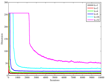
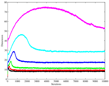
Figure 5.4: Plots of the number of eigenvalues $k_{t}^{\prime}$ which are not capped at the upper bound of $1/(d-k)$ over $10000$ iterations of Warmuth and Kuzmin’s algorithm, on the $256$-dimensional Adult dataset, for the desired subspace dimension $k\in\{1,2,4,8,16,32\}$. In the left hand plot, the algorithm was started at $W^{(0)}=\left(\nicefrac{{1}}{{d}}\right)I$, while in the right plot, it was started at a random matrix with $d-k-1$ eigenvalues equal to $1/(d-k)$, and the remaining $k+1$ equal to $1/((k+1)(d-k))$. At each iteration, samples were drawn uniformly at random from the dataset, and both plots are averaged over $16$ runs.

The key idea to improving the efficiency of the update is to observe that, at every iteration, a rank-one positive-semidefinite matrix ($\eta xx^{T}$) will be subtracted from the current iterate before performing the projection, and that the projection must therefore increase the eigenvalues in order to satisfy the constraint that the eigenvalues sum to $1$—that is, it must be the case that $Z\leq 1$. Because the eigenvalues are capped at $1/(d-k)$, a consequence of this is that, typically, and in particular when the desired subspace dimension $k$ is much smaller than $d$, many of the eigenvalues of each iterate will be exactly $1/(d-k)$. Figure 5.4 experimentally illustrates this phenomenon, on the $256$-dimensional Adult dataset (more detailed experiments may be found in Chapter 6).

$\mbox{{rank1-update}}\left(d,k,k^{\prime}:\mathbb{N},U:\mathbb{R}^{d\times k^{\prime}},\sigma:\mathbb{R}^{k^{\prime}},\eta\in\mathbb{R},x:\mathbb{R}^{d}\right)$
1	$\hat{x}\leftarrow U^{T}x$; $x_{\perp}\leftarrow x-U\hat{x}$; $r\leftarrow\left\lVert{x_{\perp}}\right\rVert$;
2	$\mbox{{if }}r>0$
3		$V^{\prime},\sigma^{\prime}\leftarrow\mbox{{eig}}([\mbox{{diag}}(\sigma)+\eta\hat{x}\hat{x}^{T},\eta r\hat{x};\eta r\hat{x}^{T},\eta r^{2}+1/(d-k)])$;
4		$U^{\prime}\leftarrow[U,x_{\perp}/r]V^{\prime}$;
5	else
6		$V^{\prime},\sigma^{\prime}\leftarrow\mbox{{eig}}(\mbox{{diag}}(\sigma)+\eta\hat{x}\hat{x}^{T})$;
7		$U^{\prime}\leftarrow UV^{\prime}$;
8	$\mbox{{return }}U^{\prime},\sigma^{\prime}$;

Algorithm 5.5 Routine which computes an eigendecomposition of $W+\eta xx^{T}$ from an eigendecomposition $W=U\mbox{{diag}}(\sigma)U^{T}+(1/(d-k))(I-U)(I-U)^{T}$, where $U$ is a matrix containing $k^{\prime}$ orthonormal eigenvectors in its columns, $\sigma$ is a vector of the corresponding eigenvalues, and the eigenvalues corresponding to all eigenvectors not spanned by the columns of $U$ are exactly $1/(d-k)$. The computational cost of this algorithm is dominated by the matrix multiplication defining $U$ (line $4$ or $7$) costing $O((k^{\prime})^{2}d)$ operations.

Exploiting this observation turns out to rely on a similar technique to that used in the incremental algorithm of Section 24 in Chapter 4. The key difference is that, whereas the incremental algorithm performs a rank-1 update to a low-rank matrix, we now must perform a rank-1 update to a matrix with many eigenvalues equal to exactly $1/(d-k)$, instead of $0$. Algorithm 5.5 demonstrates the necessary modification to Algorithm 4.3. The reasoning behind this algorithm is only a little more complicated than that of Section 24. Begin by writing $W$ as:

$$W=U^{T}\mbox{diag}(\sigma)U+\frac{1}{d-k}U^{T}U$$

Here, the columns of $U\in\mathbb{R}^{d\times k^{\prime}}$ are the eigenvectors of $W$ with corresponding unbound eigenvalues in the vector $\sigma$, with all other eigenvalues being $1/(d-k)$. Defining $x_{\perp}=(I-U)(I-U)^{T}x$ as the portion of $x$ which does not lie in the span of the columns of $U$, and taking $r=\left\lVert{x_{\perp}}\right\rVert$, gives that, if $r>0$ (the $r=0$ case is trivial):

$$W+\eta xx^{T}= \left[\begin{array}[]{cc}U&\frac{x_{\perp}}{r}\end{array}\right]\left[\begin{array}[]{cc}\mbox{diag}(\sigma)+\eta U^{T}xx^{T}U&\eta rUU^{T}x\\ \eta rx^{T}UU^{T}&\frac{1}{d-k}+\eta\end{array}\right]\left[\begin{array}[]{cc}U&\frac{x_{\perp}}{r}\end{array}\right]^{T}$$

$$+\frac{1}{d-k}(I-U-\frac{x_{\perp}}{r})(I-U-\frac{x_{\perp}}{r})^{T}$$

We next take the eigendecomposition of the rank-$k^{\prime}+1$ matrix in the above equation:

$$\left[\begin{array}[]{cc}\mbox{diag}(\sigma)+\eta U^{T}xx^{T}U&\eta rUU^{T}x\\ \eta rx^{T}UU^{T}&\frac{1}{d-k}+\eta\end{array}\right]=V^{\prime}\mbox{diag}\left(\sigma^{\prime}\right)\left(V^{\prime}\right)^{T}$$

giving that:

$$W+\eta xx^{T}= \left(\left[\begin{array}[]{cc}U&\frac{x_{\perp}}{r}\end{array}\right]V^{\prime}\right)\mbox{diag}\left(\sigma^{\prime}\right)\left(\left[\begin{array}[]{cc}U&\frac{x_{\perp}}{r}\end{array}\right]V^{\prime}\right)^{T}$$

$$+\frac{1}{d-k}(I-U-\frac{x_{\perp}}{r})(I-U-\frac{x_{\perp}}{r})^{T}$$

This shows that the new vector of non-capped eigenvalues is $\sigma^{\prime}$, with the corresponding eigenvectors being:

$$U^{\prime}=\left[\begin{array}[]{cc}U&\frac{x_{\perp}}{r}\end{array}\right]V^{\prime}$$

Algorithm 5.5 performs precisely these steps (with some additional handling for the $r=0$ case).

Ultimately, the cost of finding $W^{\prime}=W+\eta xx^{T}$, and maintaining an eigendecomposition during this update, is the cost of the matrix multiplication defining the new set of eigenvectors $U^{\prime}$: $O\left(\left(k^{\prime}\right)^{2}d\right)$. Performing the projection using Algorithm 5.3 then requires an additional $O\left(k^{\prime}\log k^{\prime}\right)$ steps, since $W^{\prime}$ has $k^{\prime}+1$ distinct eigenvalues. The overall computational cost of performing a single iteration of this optimized version of Warmuth and Kuzmin’s algorithm is therefore $O\left(\left(k^{\prime}\right)^{2}d\right)$. The memory usage at each iteration is likewise dominated by the cost of storing the eigenvectors: $O(k^{\prime}d)$. Compared to the cost of performing and storing two rank-$d$ eigendecompositions per iteration, this is an extremely significant improvement.

The precise cost-per-iteration, unfortunately, depends on the quantity $k^{\prime}$, which varies from iteration-to-iteration (we will occasionally refer to this quantity as $k_{t}^{\prime}$ to emphasize this fact), and can indeed be as large as $d-1$ (or as small as $k+1$). Hence, while this is an improvement, its theoretical impact is limited. In practical terms, however, $k^{\prime}$ often tends to be quite small, particularly when the algorithm is close to convergence, as can be seen in Figure 5.4.

29   Interpretation as Mirror Descent

	Description
$\mathcal{W}\subseteq\mathcal{H}$	Feasible region (convex subset of some Hilbert space $\mathcal{H}$)
$\mathcal{F}$	Set of convex loss functions with bounded subgradients
$\Psi$	Distance generating function
$\Psi^{*}\left(z^{*}\right)=\sup_{z}\left(\left\langle{z^{*}},{z}\right\rangle-\Psi(z)\right)$	Convex conjugate of $\Psi$
$\left\lVert{\cdot}\right\rVert_{\Psi}$	Norm with respect to which $\Psi$ is $1$-strongly convex
$\left\lVert{\cdot}\right\rVert_{\Psi^{*}}$	Dual norm of $\left\lVert{\cdot}\right\rVert_{\Psi}$
$\Delta_{\Psi}\left(z\|z^{\prime}\right)=\Psi(z)-\Psi(z^{\prime})-\left\langle{\Delta\Psi(z^{\prime})},{z-z^{\prime}}\right\rangle$	Bregman divergence derived from $\Psi$

Table 5.6: Summary of mirror descent notation introduced in Section 29.

In this section, we will present the online mirror descent algorithm, give a bound on its convergence rate, adapt it to the stochastic setting using an online-to-batch conversion, and finally describe how it may be applied to Problem 5.2. Mirror Descent [40] is generally presented in the online setting, although we are interested exclusively in the stochastic setting, and will adjust our presentation of mirror descent, and its application to Warmuth and Kuzmin’s algorithm, accordingly. However, it should be noted that, despite our preference for the stochastic setting, the algorithms of this section could be presented in the online setting with little difficulty.

Whereas in the stochastic setting the learning task is essentially to fit a hypothesis to an unknown data distribution based on some number of independent samples drawn from this distribution, the online setting is best viewed as a repeated game, in which the “learner” and “adversary” alternatingly choose a hypothesis and a loss function, respectively, with the goal of the learner being to suffer cumulative loss little higher than that achieved by the best fixed hypothesis, and the adversary, true to its name, is free to choose loss functions adversarially. We here base our treatment of mirror descent on that of Srebro et al. [57], in which, more formally, for a hypothesis space $\mathcal{W}$ and set of candidate loss functions $\mathcal{F}$, the learner is taken to be a function $\mathcal{A}:\bigcup_{t\in\mathbb{N}}\mathcal{F}^{t}\rightarrow\mathcal{W}$—i.e. for any sequence of $0$ or more loss functions (provided by the adversary at previous steps), the learner outputs a hypothesis in $\mathcal{W}$. At the $t$th step, after the learner has chosen a hypothesis $w_{t}=\mathcal{A}\left(f_{1},f_{2},\dots,f_{t-1}\right)$, the adversary chooses a new loss function $f_{t}\in\mathcal{F}$, and the learner suffers loss $f_{t}\left(w_{t}\right)$. The performance of $\mathcal{A}$ is measured in terms of the online regret:

$$R_{T}=\frac{1}{T}\sum_{t=1}^{T}f_{t}\left(w_{t}\right)-\inf_{w\in\mathcal{W}}\frac{1}{T}\sum_{t=1}^{T}f_{t}\left(w\right)$$ (5.8)

The lower the regret, the closer the learner is to performing as well as the best fixed hypothesis $w$.

While the treatment of Srebro et al. [57] is far more general, we are interested only in the setting in which $\mathcal{W}$ is a convex subset of a Hilbert space $\mathcal{H}$, and the loss functions $f\in\mathcal{F}$ are convex with bounded subgradients. In order to define the mirror descent update, we must provide a distance generating function (d.g.f.) $\Psi:\mathcal{H}\rightarrow\mathbb{R}$, which we take to be differentiable, nonnegative and $1$-strongly convex with respect to a norm $\left\lVert{\cdot}\right\rVert_{\Psi}$:

$$\left\langle{\nabla\Psi\left(z\right)-\nabla\Psi\left(z^{\prime}\right)},{z-z^{\prime}}\right\rangle\geq\left\lVert{z-z^{\prime}}\right\rVert_{\Psi}^{2}$$ (5.9)

Both the norm $\left\lVert{\cdot}\right\rVert_{\Psi}$ and its dual $\left\lVert{\cdot}\right\rVert_{\Psi^{*}}$ are relevant for the analysis, but not for the specification of the algorithm itself. The fact that mirror descent is parameterized by a distance generating function is the essence of its generality—as we will see, choosing different $\Psi$s results in different update rules, and yields different convergence rates (depending on other properties of the problem under consideration). In the vector case, the two most important distance generating functions are the squared Euclidean norm, for which mirror descent becomes nothing but stochastic gradient descent, and the negative Shannon entropy, which gives the multiplicative-weights algorithm. In the matrix setting (which is our area of interest), the analogues of these two cases are the squared Frobenius norm and negative von Neumann entropy, respectively. There are literally infinite possibilities, however, and the fact that they can all be unified under a common framework is remarkable, and significantly simplifies the creation, interpretation and analysis of new online and stochastic-gradient-type algorithms.

We do need some additional pieces beyond $\Psi$ in order to fully specify the mirror descent update algorithm—for one, we need its convex conjugate $\Psi^{*}$, which we assume to be differentiable:

$$\Psi^{*}\left(z^{*}\right)=\sup_{z}\left(\left\langle{z^{*}},{z}\right\rangle-\Psi\left(z\right)\right)$$ (5.10)

and the Bregman divergence defined by $\Psi$:

$$\Delta_{\Psi}\left(z\|z^{\prime}\right)=\Psi\left(z\right)-\Psi\left(z^{\prime}\right)-\left\langle{\nabla\Psi\left(z^{\prime}\right)},{z-z^{\prime}}\right\rangle$$ (5.11)

Table 5.6 summarizes the above notation and assumptions. With these pieces in place, we may state the mirror descent update, and give Srebro et al. [57]’s bound on its convergence rate:

Lemma 5.12.

In the setting described above, define the algorithm $\mathcal{A}$ using the following update rule:

$$w_{t+1}^{\prime}= \nabla\Psi^{*}\left(\nabla\Psi\left(w_{t}\right)-\eta\nabla f_{t}\left(w_{t}\right)\right)$$

$$w_{t+1}= \underset{w\in\mathcal{W}}{\operatorname{argmin}}\Delta_{\Psi}\left(w\|w^{\prime}\right)$$

with the step size $\eta=\sqrt{B/T}$ where $\sup_{w\in\mathcal{W}}\Psi\left(w\right)\leq B$. Then:

$$R_{T}\leq 2\sqrt{B/T}$$

provided that $\frac{1}{T}\sum_{t=1}^{T}\left\lVert{\nabla f_{t}\left(w_{t}\right)}\right\rVert_{\Psi^{*}}^{2}\leq 1$.

Proof.

This is Lemma 2 of Srebro et al. [57]. ∎

We may adapt this result to the stochastic setting very straightforwardly, by assuming that the convex loss functions $f_{t}$, instead of being chosen adversarially, are drawn i.i.d. from some unknown distribution with $\mathbb{E}\left[f_{t}\left(w\right)\right]=f\left(w\right)$. In this case, taking expectations of the above regret bound and using the definition of Equation 5.8:

$$\mathbb{E}\left[\frac{1}{T}\sum_{t=1}^{T}f_{t}\left(w_{t}\right)\right]\leq \mathbb{E}\left[\inf_{w\in\mathcal{W}}\frac{1}{T}\sum_{t=1}^{T}f_{t}\left(w\right)\right]+\frac{2B}{\sqrt{T}}$$

$$\mathbb{E}\left[\frac{1}{T}\sum_{t=1}^{T}f\left(w_{t}\right)\right]\leq \inf_{w\in\mathcal{W}}f\left(w\right)+\frac{2B}{\sqrt{T}}$$

Let $\hat{w}$ be sampled uniformly from the set $\left\{w_{1},\dots,w_{T}\right\}$ [11]. Then:

$$\mathbb{E}\left[f\left(\hat{w}\right)\right]\leq\inf_{w\in\mathcal{W}}f\left(w\right)+\frac{2B}{\sqrt{T}}$$ (5.13)

Hence, in the stochastic setting, we may find a single hypothesis satisfying bound of Lemma 5.12 in expectation.

In the particular case of Warmuth and Kuzmin’s convex relaxation of the stochastic PCA objective (Problem 5.2), the hypothesis space $\mathcal{W}$ is the set of positive semidefinite matrices satisfying the constraints. While the above has all been written in terms of vector operations, for the purposes of defining the strong convexity of $\Psi$, convex conjugate $\Psi^{*}$ and the Bregman divergence $\Delta_{\Psi}\left(x\|x^{\prime}\right)$ (Equations 5.9, 5.10 and 5.11, respectively) we may treat the matrices as vectors by using Frobenius inner products $\left\langle{W},{W^{\prime}}\right\rangle_{F}=\sum_{i,j}W_{i,j}W_{i,j}^{\prime}=\operatorname{tr}WW^{\prime}$ (this holds for symmetric $W$ and $W^{\prime}$). Defining $f_{t}\left(W\right)=x_{t}^{T}Wx_{t}$ where $x_{t}$ is sampled i.i.d. from the data distribution $\mathcal{D}$ suffices to express optimization of a relaxed stochastic PCA objective as an instance of mirror descent. It only remains to specify the distance generating function $\Psi$ and norm $\left\lVert{\cdot}\right\rVert_{\Psi}$, and verify that the conditions of Lemma 5.12 are satisfied.

29.1   Negative von Neumann d.g.f.

We will now show that Warmuth and Kuzmin’s algorithm is nothing but mirror descent applied to Problem 5.2 using a shifted-and-scaled version of the negative von Neumann entropy $-S\left(W\right)=\operatorname{tr}W\ln W$:

$$\Psi_{vN}\left(W\right)=\alpha\left(\operatorname{tr}W\ln W-\beta\right)$$

We choose the scaling constant $\alpha$ in such a way as to insure that $\Psi_{vN}$ is $1$-strongly convex with respect to some norm, and $\beta$ to minimize $\Psi_{vN}$ while maintaining nonnegativity (i.e. so as to minimize the bound of Lemma 5.12).

Before stating the mirror descent update which results from this choice of distance generating function, we must verify that it satisfies the conditions outlined earlier in this section. In order to show strong convexity, observe that $-\nabla S\left(W\right)=I+\ln W$, and so:

$$\left\langle{\nabla\left(-S\left(W\right)\right)-\nabla\left(-S\left(W^{\prime}\right)\right)},{W-W^{\prime}}\right\rangle_{F}$$

$$=\operatorname{tr}W\left(\ln W-\ln W^{\prime}\right)+\operatorname{tr}W^{\prime}\left(\ln W^{\prime}-\ln W\right)$$

$$=D_{KL}\left(W\|W^{\prime}\right)+D_{KL}\left(W^{\prime}\|W\right)$$

where $D_{KL}$ is the quantum relative entropy (Equation 5.5). By the quantum Pinsker inequality [26, 24], $D_{KL}\left(W\|W^{\prime}\right)\geq 2\left\lVert{W-W^{\prime}}\right\rVert_{1}^{2}$, where $\left\lVert{\cdot}\right\rVert_{1}$ is the Schatten $1$-norm (i.e. the trace norm, the sum of the absolute eigenvalues of its argument):

$$\left\langle{\nabla\Psi_{vN}\left(W\right)-\nabla\Psi_{vN}\left(W^{\prime}\right)},{W-W^{\prime}}\right\rangle_{F}\geq 4\left\lVert{W-W^{\prime}}\right\rVert_{1}^{2}$$

Hence, $-S\left(W\right)/4$ is $1$-strongly convex, showing that we should take $\alpha=1/4$.

In order to find $\beta$, we should note that, over the feasible region $\mathcal{W}$ of 5.2, the maximum entropy (and therefore minimum negative entropy) is achieved by the “uniform” matrix $W=I/d$, for which $-S\left(I/d\right)=-\ln d$. Therefore, the largest value of $\beta$ which ensures nonnegativity of $\Psi_{vN}$ on the feasible regions is $\beta=-\ln d$. Hence:

$$\Psi_{vN}\left(W\right)=\frac{1}{4}\left(\operatorname{tr}W\ln W+\ln d\right)$$ (5.14)

What remains is now a simple matter of plugging this choice of $\Psi$ into Lemma 5.12, although some additional work is required in order to simplify the update and projection steps. The update and convergence rate are given by the following lemma: lem:pca-warmuth:convergence-vN

If we apply the mirror descent algorithm to Problem 5.2 with the distance generating function of Equation 5.14, then the update equation is:

$$W^{\left(t+1\right)}=\mathcal{P}_{\textrm{RE}}\left(\exp\left(\ln W^{\left(t\right)}-\eta x_{t}x_{t}^{T}\right)\right)$$

where $\mathcal{P}_{\textrm{RE}}\left(\cdot\right)$ projects its argument onto the constraints of Problem 5.2 with respect to the quantum relative entropy $D_{KL}\left(W\|W^{\prime}\right)=\operatorname{tr}W\left(\ln W-\ln W^{\prime}\right)$. Furthermore, if we perform $T$ iterations with step size $\eta=\frac{2}{\sqrt{T}}\sqrt{\frac{k}{d-k}}$, then:

$$\left(d-k\right)\mathbb{E}_{x\sim\mathcal{D}}\left[x^{T}\hat{W}x\right]\leq\left(d-k\right)\inf_{W\in\mathcal{W}}\mathbb{E}_{x\sim\mathcal{D}}\left[x^{T}Wx\right]+\sqrt{\frac{k\left(d-k\right)}{T}}$$

Here, $\hat{W}$ is sampled uniformly from the set $\left\{W^{\left(1\right)},W^{\left(2\right)},\dots,W^{\left(T\right)}\right\}$. We have already shown that $\Psi_{vN}$ is nonnegative and $1$-strongly convex with respect to $\left\lVert{\cdot}\right\rVert_{1}$. The convex conjugate of $\Psi_{vN}$ satisfies:

$$\Psi_{vN}^{*}\left(W^{*}\right)=\sup_{W}\left(\left\langle{W^{*}},{W}\right\rangle_{F}-\Psi_{vN}\left(W\right)\right)$$

differentiating the expression inside the supremum, and setting the result equal to zero, gives that $0=W^{*}-\frac{1}{4}\left(I+\ln W\right)$, so the $W$ maximizing the supremum defining $\Psi_{vN}^{*}$ is $W=\exp\left(4W^{*}-I\right)$, and so:

$$\Psi_{vN}^{*}\left(W^{*}\right)=\frac{1}{4}\left(\operatorname{tr}\exp\left(4W^{*}-I\right)-\ln d\right)$$

Because $\nabla\Psi_{vN}\left(W\right)=\frac{1}{4}\left(I+\ln W\right)$, $\nabla\Psi_{vN}^{*}\left(W^{*}\right)=\exp\left(4W^{*}-I\right)$, and the stochastic objective $f_{t}\left(W\right)=x_{t}^{T}Wx_{t}$ has gradient $x_{t}x_{t}^{T}$, the mirror descent update (Lemma 5.12) is:

$$W^{\left(t+1\right)}=\mathcal{P}_{\textrm{RE}}\left(\exp\left(\ln W-4\eta^{\prime}x_{t}x_{t}^{T}\right)\right)$$

where $\mathcal{P}_{\textrm{RE}}\left(\cdot\right)$ projects its argument onto $\mathcal{W}$ with respect to the Bregman divergence:

$$\Delta_{\Psi_{vN}}\left(W\|W^{\prime}\right)= \Psi_{vN}\left(W\right)-\Psi_{vN}\left(W^{\prime}\right)-\left\langle{\nabla\Psi_{vN}\left(W^{\prime}\right)},{W-W^{\prime}}\right\rangle_{F}$$

$$= \frac{1}{4}\operatorname{tr}W\ln W-\frac{1}{4}\operatorname{tr}W^{\prime}\ln W^{\prime}-\frac{1}{4}\left\langle{I+\ln W^{\prime}},{W-W^{\prime}}\right\rangle_{F}$$

$$= \frac{1}{4}D_{KL}\left(W\|W^{\prime}\right)-\frac{1}{4}\operatorname{tr}W+\frac{1}{4}\operatorname{tr}W^{\prime}$$

Because $\operatorname{tr}W=1$ on the feasible set and $\operatorname{tr}W^{\prime}$ is a constant, the last two terms may be ignored while performing the projection, showing that $\mathcal{P}_{\mathrm{RE}}\left(\cdot\right)$ projects its argument onto the feasible set with respect to the quantum relative entropy. Because $\left\lVert{\cdot}\right\rVert_{\Psi}$ is the trace norm, $\left\lVert{\cdot}\right\rVert_{\Psi^{*}}$ is the Schatten $\infty$-norm, and $\left\lVert{x}\right\rVert\leq 1$ with probability $1$ by assumption (Section 21 in Chapter 4), so $\mathbb{E}_{x\sim\mathcal{D}}\left[\left\lVert{xx^{T}}\right\rVert_{\Psi^{*}}^{2}\right]=1$. Furthermore, the maximum value of $\Psi_{vN}$ is achieved on the corners of the matrix simplex constraints:

$$\sup_{W\in\mathcal{W}}\Psi_{vN}\left(W\right)= \frac{1}{4}\left(\ln\frac{1}{d-k}+\ln d\right)$$

$$= \frac{1}{4}\ln\frac{d}{d-k}$$

$$\leq \frac{1}{4}\cdot\frac{k}{d-k}$$

so Equation 5.13 yields that, with the step size $\eta^{\prime}=\frac{1}{2\sqrt{T}}\sqrt{\frac{k}{d-k}}$:

$$\mathbb{E}_{x\sim\mathcal{D}}\left[x^{T}\hat{W}x\right]\leq\inf_{W\in\mathcal{W}}\mathbb{E}_{x\sim\mathcal{D}}\left[x^{T}Wx\right]+\frac{1}{\sqrt{T}}\sqrt{\frac{k}{d-k}}$$

We define $\eta=4\eta^{\prime}$ to complete the proof. Unfortunately, while this result demonstrates that Warmuth and Kuzmin’s algorithm is an instance of mirror descent, the proved convergence rate is significantly worse than that which they proved “from scratch” (Equation 5.6). In the first place, it is “non-optimistic”, in that it always gives a $O\left(\sqrt{k(d-k)/T}\right)$ rate, while Warmuth and Kuzmin’s analysis improves towards $O(k/T)$ if $L^{*}$ is small. More importantly, this mirror descent-based bound contains an additional $\sqrt{d-k}$ factor even when $L^{*}$ is large.

The fact that Warmuth and Kuzmin’s algorithm is nothing but mirror descent on a particular convex relaxation of the PCA objective, however, does provide a simple “recipe” for creating other PCA optimization algorithms—we may consider different convex relaxations, and different distance generating functions. In Chapter 6, one such algorithm will be presented, for which a straightforwardly-derived convergence rate is non-optimistic, but does not contain the troublesome $\sqrt{d-k}$ factor.

Collaborators:

The novel content of this chapter (Sections 28.2 and 29) was performed jointly with Raman Arora, Karen Livescu and Nathan Srebro.

30   Proofs for Chapter 5

lem:pca-warmuth:projection

Let $W^{\prime}\in\mathbb{R}^{d\times d}$ be a symmetric matrix, with eigenvalues $\sigma_{1}^{\prime},\dots,\sigma_{d}^{\prime}$ and associated eigenvectors $v_{1}^{\prime},\dots,v_{d}^{\prime}$. If $W=\mathcal{P}_{\textrm{RE}}\left(W^{\prime}\right)$ projects $W^{\prime}$ onto the feasible region of Problem 5.2 with respect to the quantum relative entropy (Equation 5.5), then $W$ will be the unique feasible matrix which has the same set of eigenvectors as $W^{\prime}$, with the associated eigenvalues $\sigma_{1},\dots,\sigma_{d}$ satisfying:

$$\sigma_{i}=\min\left(\frac{1}{d-k},\frac{\sigma_{i}^{\prime}}{Z}\right)$$

with $Z\in\mathbb{R}^{+}$ being chosen in such a way that:

$$\sum_{i=1}^{d}\sigma_{i}=1$$

The problem of finding $W$ can be written in the form of a convex optimization problem as:

$$\mbox{minimize}: \ \ D_{KL}\left(W\|W^{\prime}\right)$$

$$\mbox{subject to}: W\succeq 0,\left\lVert{W}\right\rVert_{2}\leq\frac{1}{d-k},\operatorname{tr}W=1$$

The Hessian of the objective function is $M^{-}1$, which is positive definite for positive definite $M$, and all feasible $M$ are positive definite. Hence, the objective is strongly convex. The constraints are also convex, so this problem must have a unique solution. Letting $\sigma_{1},\dots,\sigma_{d}$ and $v_{1},\dots,v_{d}$ be the eigenvalues and associated eigenvectors of $W$, we may write the KKT first-order optimality conditions [6] as:

$$0= \nabla D_{KL}\left(W\|W^{\prime}\right)+\mu I-\sum_{i=1}^{d}\alpha_{i}v_{i}v_{i}^{T}+\sum_{i=1}^{d}\beta_{i}v_{i}v_{i}^{T}$$

$$= I+\ln W-\ln W^{\prime}+\mu I-\sum_{i=1}^{d}\alpha_{i}v_{i}v_{i}^{T}+\sum_{i=1}^{d}\beta_{i}v_{i}v_{i}^{T}$$ (5.15)

where $\mu$ is the Lagrange multiplier for the constraint $\operatorname{tr}W=1$, and $\alpha_{i},\beta_{i}\geq 0$ are the Lagrange multipliers for the constraints $W\succeq 0$ and $\left\lVert{W}\right\rVert_{2}\leq 1/(d-k)$, respectively. The complementary slackness conditions are that $\alpha_{i}\sigma_{i}=\beta_{i}\left(\sigma_{i}-1/(d-k)\right)=0$. In addition, $W$ must be feasible.

Because every term in Equation 5.15 except for $W^{\prime}$ has the same set of eigenvectors as $W$, it follows that an optimal $W$ must have the same set of eigenvectors as $W^{\prime}$, so we may take $v_{i}=v_{i}^{\prime}$, and write Equation 5.15 purely in terms of the eigenvalues:

$$\sigma_{i}=\frac{\exp\alpha_{i}}{\exp\beta_{i}}\left(\frac{\sigma_{i}}{\exp\left(1+\mu\right)}\right)$$

By complementary slackness and feasibility with respect to the constraints $0\leq\sigma_{i}\leq 1/(d-k)$, if $0\leq\sigma_{i}^{\prime}/\exp\left(1+\mu\right)\leq 1/(d-k)$, then $\sigma_{i}=\sigma_{i}^{\prime}/\exp\left(1+\mu\right)$. Otherwise, $\alpha_{i}$ and $\beta_{i}$ will be chosen so as to clip $\sigma_{i}$ to the active constraint:

$$\sigma_{i}=\max\left(0,\min\left(\frac{1}{d-k},\frac{\sigma_{i}}{\exp\left(1+\mu\right)}\right)\right)$$

Because $\exp\left(1+\mu\right)$ is nonnegative, clipping with $0$ is unnecessary. Primal feasibility with respect to the constraint $\operatorname{tr}W=1$ gives that $\mu$ must be chosen in such a way that $\operatorname{tr}W=1$, completing the proof. lem:pca-warmuth:convergence-vN

If we apply the mirror descent algorithm to Problem 5.2 with the distance generating function of Equation 5.14, then the update equation is:

$$W^{\left(t+1\right)}=\mathcal{P}_{\textrm{RE}}\left(\exp\left(\ln W^{\left(t\right)}-\eta x_{t}x_{t}^{T}\right)\right)$$

where $\mathcal{P}_{\textrm{RE}}\left(\cdot\right)$ projects its argument onto the constraints of Problem 5.2 with respect to the quantum relative entropy $D_{KL}\left(W\|W^{\prime}\right)=\operatorname{tr}W\left(\ln W-\ln W^{\prime}\right)$. Furthermore, if we perform $T$ iterations with step size $\eta=\frac{2}{\sqrt{T}}\sqrt{\frac{k}{d-k}}$, then:

$$\left(d-k\right)\mathbb{E}_{x\sim\mathcal{D}}\left[x^{T}\hat{W}x\right]\leq\left(d-k\right)\inf_{W\in\mathcal{W}}\mathbb{E}_{x\sim\mathcal{D}}\left[x^{T}Wx\right]+\sqrt{\frac{k\left(d-k\right)}{T}}$$

Here, $\hat{W}$ is sampled uniformly from the set $\left\{W^{\left(1\right)},W^{\left(2\right)},\dots,W^{\left(T\right)}\right\}$. We have already shown that $\Psi_{vN}$ is nonnegative and $1$-strongly convex with respect to $\left\lVert{\cdot}\right\rVert_{1}$. The convex conjugate of $\Psi_{vN}$ satisfies:

$$\Psi_{vN}^{*}\left(W^{*}\right)=\sup_{W}\left(\left\langle{W^{*}},{W}\right\rangle_{F}-\Psi_{vN}\left(W\right)\right)$$

differentiating the expression inside the supremum, and setting the result equal to zero, gives that $0=W^{*}-\frac{1}{4}\left(I+\ln W\right)$, so the $W$ maximizing the supremum defining $\Psi_{vN}^{*}$ is $W=\exp\left(4W^{*}-I\right)$, and so:

$$\Psi_{vN}^{*}\left(W^{*}\right)=\frac{1}{4}\left(\operatorname{tr}\exp\left(4W^{*}-I\right)-\ln d\right)$$

Because $\nabla\Psi_{vN}\left(W\right)=\frac{1}{4}\left(I+\ln W\right)$, $\nabla\Psi_{vN}^{*}\left(W^{*}\right)=\exp\left(4W^{*}-I\right)$, and the stochastic objective $f_{t}\left(W\right)=x_{t}^{T}Wx_{t}$ has gradient $x_{t}x_{t}^{T}$, the mirror descent update (Lemma 5.12) is:

$$W^{\left(t+1\right)}=\mathcal{P}_{\textrm{RE}}\left(\exp\left(\ln W-4\eta^{\prime}x_{t}x_{t}^{T}\right)\right)$$

where $\mathcal{P}_{\textrm{RE}}\left(\cdot\right)$ projects its argument onto $\mathcal{W}$ with respect to the Bregman divergence:

$$\Delta_{\Psi_{vN}}\left(W\|W^{\prime}\right)= \Psi_{vN}\left(W\right)-\Psi_{vN}\left(W^{\prime}\right)-\left\langle{\nabla\Psi_{vN}\left(W^{\prime}\right)},{W-W^{\prime}}\right\rangle_{F}$$

$$= \frac{1}{4}\operatorname{tr}W\ln W-\frac{1}{4}\operatorname{tr}W^{\prime}\ln W^{\prime}-\frac{1}{4}\left\langle{I+\ln W^{\prime}},{W-W^{\prime}}\right\rangle_{F}$$

$$= \frac{1}{4}D_{KL}\left(W\|W^{\prime}\right)-\frac{1}{4}\operatorname{tr}W+\frac{1}{4}\operatorname{tr}W^{\prime}$$

Because $\operatorname{tr}W=1$ on the feasible set and $\operatorname{tr}W^{\prime}$ is a constant, the last two terms may be ignored while performing the projection, showing that $\mathcal{P}_{\mathrm{RE}}\left(\cdot\right)$ projects its argument onto the feasible set with respect to the quantum relative entropy. Because $\left\lVert{\cdot}\right\rVert_{\Psi}$ is the trace norm, $\left\lVert{\cdot}\right\rVert_{\Psi^{*}}$ is the Schatten $\infty$-norm, and $\left\lVert{x}\right\rVert\leq 1$ with probability $1$ by assumption (Section 21 in Chapter 4), so $\mathbb{E}_{x\sim\mathcal{D}}\left[\left\lVert{xx^{T}}\right\rVert_{\Psi^{*}}^{2}\right]=1$. Furthermore, the maximum value of $\Psi_{vN}$ is achieved on the corners of the matrix simplex constraints:

$$\sup_{W\in\mathcal{W}}\Psi_{vN}\left(W\right)= \frac{1}{4}\left(\ln\frac{1}{d-k}+\ln d\right)$$

$$= \frac{1}{4}\ln\frac{d}{d-k}$$

$$\leq \frac{1}{4}\cdot\frac{k}{d-k}$$

so Equation 5.13 yields that, with the step size $\eta^{\prime}=\frac{1}{2\sqrt{T}}\sqrt{\frac{k}{d-k}}$:

$$\mathbb{E}_{x\sim\mathcal{D}}\left[x^{T}\hat{W}x\right]\leq\inf_{W\in\mathcal{W}}\mathbb{E}_{x\sim\mathcal{D}}\left[x^{T}Wx\right]+\frac{1}{\sqrt{T}}\sqrt{\frac{k}{d-k}}$$

We define $\eta=4\eta^{\prime}$ to complete the proof.

The Capped MSG Algorithm

31   Overview

In Chapter 4, two iterative techniques for performing stochastic PCA, the stochastic power method and the incremental algorithm (Sections 23 and 24, respectively), were discussed which both perform a very small amount of computation at each iteration, but for which no good theoretical guarantees are known. The former converges with probability $1$, but at an unknown rate, while for the latter there exist distributions for which it will converge to a suboptimal solution with a high probability.

The algorithm discussed in Chapter 5, originally due to Warmuth and Kuzmin [60], is different in both of these respects: a very good bound on its convergence rate is known, but it suffers from a very high—in some cases prohibitively high—cost per iteration.

Our goal in this chapter is to present an algorithm which combines the strengths of both of these types of approaches. We begin in Section 32 by proposing an algorithm, called Matrix Stochastic Gradient (MSG), which yields updates very similar to the incremental algorithm, but for which we can give a theoretical bound on how many iterations are needed to converge to an $\epsilon$-suboptimal solution. In a sense, this algorithm is a “cross” between the incremental algorithm and Warmuth and Kuzmin’s algorithm, in that its updates are similar in form to the former, while the theoretical convergence bound on its performance is similar to (albeit slightly worse than) that of the latter. Like Warmuth and Kuzmin’s algorithm, MSG is designed to optimize a convex relaxation of the PCA optimization problem, and can theoretically have the same unacceptably high computational cost per iteration.

In order to address this, in Section 33 we will introduce a variant of MSG, called “capped MSG”, which introduces an explicit rank constraint in the spirit of the incremental algorithm, but does so far more safely, in that the resulting algorithm is much less likely to “get stuck”. We believe that the capped MSG algorithm combines the speed of the incremental algorithm with most of the reliability of MSG, yielding a “best of both worlds” approach. This chapter will conclude in Section 34 with an experimental comparison of the algorithms introduced in this chapter with most of those discussed in Chapters 4 and 5.

32   Matrix Stochastic Gradient (MSG)

	Computation	Memory	Convergence
SAA	$nd^{2}$	$d^{2}$	$\sqrt{\frac{k}{n}}$
SAA (Coppersmith-Winograd)	$nd^{1.3727}$	$d^{2}$	$\sqrt{\frac{k}{n}}$
Stochastic Power Method	$Tkd$	$kd$	w.p. $1$
Incremental	$Tk^{2}d$	$kd$	no
Warmuth & Kuzmin	$\sum_{t=1}^{T}\left(k_{t}^{\prime}\right)^{2}d$	$\max_{t\in\{1,\dots,T\}}k_{t}^{\prime}d$	$\sqrt{\frac{L^{*}k}{T}}+\frac{k}{T}$
MSG	$\sum_{t=1}^{T}\left(k_{t}^{\prime}\right)^{2}d$	$\max_{t\in\{1,\dots,T\}}k_{t}^{\prime}d$	$\sqrt{\frac{k}{T}}$
Capped MSG	$TK^{2}d$	$Kd$	testable

Table 6.1: Summary of results from Chapters 4 and 5, as well as Lemma LABEL:lem:pca-capped-msg:rate. All bounds are given up to constant factors. The “Convergence” column contains bounds on the suboptimality of the solution—i.e. the difference between the total variance captured by the rank-$k$ subspace found by the algorithm, and the best rank-$k$ subspace with respect to the data distribution $\mathcal{D}$ (the objective in Chapter 5 is scaled by a factor of $d-k$ relative to the other objectives—we have corrected for this here). MSG enjoys a convergence rate which differs from that of Warmuth and Kuzmin’s algorithm only in that it is non-optimistic.

One technique which one could use to optimize the $M$-based objective of Problem 4.2 in Chapter 4 is projected stochastic gradient descent. On the PCA problem, SGD will perform the following steps at each iteration:

$$M^{(t+1)}=\mathcal{P}\left(M^{(t)}+\eta_{t}x_{t}x_{t}^{T}\right)$$ (6.1)

here, $x_{t}x_{t}^{T}$ is the gradient of $x_{t}^{T}Mx_{t}$, $\eta_{t}$ is a step size, and $\mathcal{P}\left(\cdot\right)$ projects its argument onto the feasible region with respect to the Frobenius norm.

The performance of SGD is well-understood, at least on convex problems. Unfortunately, as we have seen, while the objective function of Problem 4.2 is linear (and therefore both convex and concave), the constraints are non-convex. For this reason, performing SGD on this objective is inadvisable—as was the case for the incremental algorithm, it is very easy to construct a distribution $\mathcal{D}$ on which it would “get stuck”.

Fortunately, this non-convexity problem can be addressed using the same technique as was successful in Section 27 of Chapter 5: we instead solve a convex relaxation of the problem in which the feasible region has been replaced with its convex hull:

$$\mbox{maximize}: \ \ \mathbb{E}_{x\sim\mathcal{D}}\left[x^{T}Mx\right]$$ (6.2)

$$\mbox{subject to}: \ \ M\in\mathbb{R}^{d\times d},0\preceq M\preceq I,\operatorname{tr}M=k.$$

This objective is quite similar to that optimized by Warmuth and Kuzmin [60] (compare to Problem 5.2 in Chapter 5)—aside from scaling, the main difference is that their objective seeks a $(d-k)$-dimensional minimal subspace, rather than a $k$-dimensional maximal subspace.

The SGD update equation on this objective is simply Equation 6.1 again, with the difference being that the projection is now performed onto the (convex) constraints of Problem 6.2. We call the resulting algorithm Matrix Stochastic Gradient (MSG). We could analyze MSG using a mirror descent-based analysis similar to that of Section 29 in Chapter 5 (the distance generating function would be the squared Frobenius norm). Unlike Warmuth and Kuzmin’s algorithm, however, a direct analysis is much simpler and more straightforward:

lem:pca-capped-msg:rate

Suppose that we perform $T$ iterations of MSG on Problem 6.2, with step size $\eta=2\sqrt{\frac{k}{T}}$. Further suppose WLOG that $\mathbb{E}_{x\sim\mathcal{D}}\left[\left\lVert{x}\right\rVert^{4}\right]\leq 1$. Then:

$$\mathbb{E}_{x\sim\mathcal{D}}\left[x^{T}M^{*}x-x^{T}\bar{M}x\right]\leq 2\sqrt{\frac{k}{T}}$$

where $\bar{M}=\frac{1}{T}\sum_{t=1}^{T}M^{(t)}$ is the average of the iterates, and $M^{*}$ is the optimum (a rank $k$ projection matrix which projects onto the maximal $k$ eigenvectors of the second-moment matrix of $\mathcal{D}$). (Based on Lemma 55 of Sridharan [58], which in turn is based on Nemirovski and Yudin [40]) Define $\tilde{M}^{(t+1)}=M^{(t)}+\eta x_{t}x_{t}^{T}$, and observe that:

$$\eta\left(\sum_{t=1}^{T}x_{t}^{T}M^{*}x_{t}-\sum_{t=1}^{T}x_{t}^{T}M^{(t)}x_{t}\right)$$

$$=\sum_{t=1}^{T}\left\langle{\eta x_{t}x_{t}^{T}},{M^{*}-M^{(t)}}\right\rangle_{F}$$

$$=\frac{1}{2}\sum_{t=1}^{T}\left(\eta^{2}\left\lVert{x_{t}}\right\rVert^{4}+\left\lVert{M^{*}-M^{(t)}}\right\rVert_{F}^{2}-\left\lVert{M^{*}-\tilde{M}^{(t+1)}}\right\rVert_{F}^{2}\right)$$

$$\leq\frac{1}{2}\sum_{t=1}^{T}\left(\eta^{2}\left\lVert{x_{t}}\right\rVert^{4}+\left\lVert{M^{*}-M^{(t)}}\right\rVert_{F}^{2}-\left\lVert{M^{*}-M^{(t+1)}}\right\rVert_{F}^{2}\right)$$

$$\leq\frac{\eta^{2}}{2}\sum_{t=1}^{T}\left\lVert{x_{t}}\right\rVert^{4}+\frac{1}{2}\left\lVert{M^{*}-M^{(1)}}\right\rVert_{F}^{2}$$

Dividing through by $\eta T$, taking expectations (observe that $x_{t}$ and $M^{(t)}$ are conditionally independent), and using the bounds $\mathbb{E}_{x\sim\mathcal{D}}\left[\left\lVert{x}\right\rVert^{4}\right]\leq 1$ and $\left\lVert{M^{*}-M^{(1)}}\right\rVert_{F}^{2}\leq 4k$ ($2\sqrt{k}$ bounds the diameter of the feasible region) gives that:

$$\mathbb{E}_{x\sim\mathcal{D}}\left[xM^{*}x-x\bar{M}x\right]\leq\frac{\eta}{2}+\frac{2k}{\eta T}.$$

Choosing $\eta=2\sqrt{\frac{k}{T}}$ completes the proof. Comparing this convergence rate to that of Warmuth and Kuzmin’s algorithm (Equation 5.6 in Chapter 5) shows that the only difference between the two is that Warmuth and Kuzmin’s algorithm enjoys an “optimistic” rate, while MSG does not—if the desired level of suboptimality is of roughly the same order as the optimal compression loss $L^{*}$ (i.e. the problem is “easy”), then the algorithm will converge at a roughly $1/T$ rate. On more difficult problem instances, Warmuth and Kuzmin’s algorithm will match the $1/\sqrt{T}$ rate of MSG.

In addition to the relationship to Warmuth and Kuzmin’s algorithm, MSG’s update is strikingly similar to that of the incremental algorithm (see Section 24 in Chapter 4). Both add $xx^{T}$ to the current iterate, and then perform a projection. The most significant difference, from a practical standpoint, is that while the iterates of the incremental algorithm will never have rank larger than $k$, each MSG iterate may have rank as large as $d$ (although it will typically be much lower). A consequence of this is that, despite the fact that Lemma LABEL:lem:pca-capped-msg:rate can be used to bound the number of iterations required to reach $\epsilon$-suboptimality, each iteration may be so computationally expensive that the algorithm is still impractical. In Section 32.2, we will discuss how this situation may be addressed.

32.1   The Projection

In order to actually perform the MSG update of Equation 6.1, we must show how one projects onto the constraints of Problem 6.2. As in Section 28.1 of Chapter 5, the first step in developing an efficient algorithm for doing so is to characterize the solution of the projection problem, which we do in the following lemma:

lem:pca-capped-msg:projection

Let $M^{\prime}\in\mathbb{R}^{d\times d}$ be a symmetric matrix, with eigenvalues $\sigma_{1}^{\prime},\dots,\sigma_{d}^{\prime}$ and associated eigenvectors $v_{1}^{\prime},\dots,v_{d}^{\prime}$. If $M=\mathcal{P}\left(M^{\prime}\right)$ projects $M^{\prime}$ onto the feasible region of Problem 6.2 with respect to the Frobenius norm, then $M$ will be the unique feasible matrix which has the same set of eigenvectors as $M^{\prime}$, with the associated eigenvalues $\sigma_{1},\dots,\sigma_{d}$ satisfying:

$$\sigma_{i}=\max\left(0,\min\left(1,\sigma_{i}^{\prime}+S\right)\right)$$

with $S\in\mathbb{R}$ being chosen in such a way that:

$$\sum_{i=1}^{d}\sigma_{i}=k$$

This is the same proof technique as was used to prove Lemma LABEL:lem:pca-warmuth:projection in Chapter 5. We begin by writing the problem of finding $M$ in the form of a convex optimization problem as:

$$\mbox{minimize}: \ \ \left\lVert{M-M^{\prime}}\right\rVert_{F}^{2}$$

$$\mbox{subject to}: \ \ 0\preceq M\preceq I,\operatorname{tr}M=k.$$

Because the objective is strongly convex, and the constraints are convex, this problem must have a unique solution. Letting $\sigma_{1},\dots,\sigma_{d}$ and $v_{1},\dots,v_{d}$ be the eigenvalues and associated eigenvectors of $M$, we may write the KKT first-order optimality conditions [6] as:

$$0=M-M^{\prime}+\mu I-\sum_{i=1}^{d}\alpha_{i}v_{i}v_{i}^{T}+\sum_{i=1}^{d}\beta_{i}v_{i}v_{i}^{T}$$ (6.3)

where $\mu$ is the Lagrange multiplier for the constraint $\operatorname{tr}M=k$, and $\alpha_{i},\beta_{i}\geq 0$ are the Lagrange multipliers for the constraints $0\preceq M$ and $M\preceq I$, respectively. The complementary slackness conditions are that $\alpha_{i}\sigma_{i}=\beta_{i}\left(\sigma_{i}-1\right)=0$. In addition, $M$ must be feasible.

Because every term in Equation 6.5 except for $M^{\prime}$ has the same set of eigenvectors as $M$, it follows that an optimal $M$ must have the same set of eigenvectors as $M^{\prime}$, so we may take $v_{i}=v_{i}^{\prime}$, and write Equation 6.5 purely in terms of the eigenvalues:

$$\sigma_{i}=\sigma_{i}^{\prime}-\mu+\alpha_{i}-\beta_{i}$$

Complementary slackness and feasibility with respect to the constraints $0\preceq M\preceq I$ gives that if $0\leq\sigma_{i}^{\prime}-\mu\leq 1$, then $\sigma_{i}=\sigma_{i}^{\prime}-\mu$. Otherwise, $\alpha_{i}$ and $\beta_{i}$ will be chosen so as to clip $\sigma_{i}$ to the active constraint:

$$\sigma_{i}=\max\left(0,\min\left(1,\sigma_{i}^{\prime}-\mu\right)\right)$$

Primal feasibility with respect to the constraint $\operatorname{tr}M=k$ gives that $\mu$ must be chosen in such a way that $\operatorname{tr}M=k$, completing the proof. This result shows that projecting onto the feasible region amounts to finding the value of $S$ such that, after shifting the eigenvalues by $S$ and clipping the results to $[0,1]$, the result is feasible.

$\mbox{{project}}\left(d,k,m:\mathbb{N},\sigma^{\prime}:\mathbb{R}^{m},\kappa^{\prime}:\mathbb{N}^{m}\right)$
1	$\sigma^{\prime},\kappa^{\prime}\leftarrow\mbox{{sort}}(\sigma^{\prime},\kappa^{\prime})$;
2	$i\leftarrow 1$; $j\leftarrow 1$; $s_{i}\leftarrow 0$; $s_{j}\leftarrow 0$; $c_{i}\leftarrow 0$; $c_{j}\leftarrow 0$;
3	$\mbox{{while }}i\leq m$
4		$\mbox{{if }}(i<j)$
5			$S\leftarrow(k-(s_{j}-s_{i})-(d-c_{j}))/(c_{j}-c_{i})$;
6			$b\leftarrow($
				$(\sigma_{i}^{\prime}+S\geq 0)\mbox{{ and }}(\sigma_{j-1}^{\prime}+S\leq 1)$
				$\mbox{{and }}((i\leq 1)\mbox{{ or }}(\sigma_{i-1}^{\prime}+S\leq 0))$
				$\mbox{{and }}((j\geq m)\mbox{{ or }}(\sigma_{j+1}^{\prime}\geq 1))$
			$)$;
7			$\mbox{{return }}S\mbox{{ if }}b$;
8		$\mbox{{if }}(j\leq m)\mbox{{ and }}(\sigma_{j}^{\prime}-\sigma_{i}^{\prime}\leq 1)$
9			$s_{j}\leftarrow s_{j}+\kappa_{j}^{\prime}\sigma_{j}^{\prime}$; $c_{j}\leftarrow c_{j}+\kappa_{j}^{\prime}$; $j\leftarrow j+1$;
10		else
11			$s_{i}\leftarrow s_{i}+\kappa_{i}^{\prime}\sigma_{i}^{\prime}$; $c_{i}\leftarrow c_{i}+\kappa_{i}^{\prime}$; $i\leftarrow i+1$;
12	return error;

Algorithm 6.2 Routine which finds the $S$ of Lemma LABEL:lem:pca-capped-msg:projection. It takes as parameters the dimension $d$, “target” subspace dimension $k$, and the number of distinct eigenvalues $m$ of the current iterate. The length-$m$ arrays $\sigma^{\prime}$ and $\kappa^{\prime}$ contain the distinct eigenvalues and their multiplicities, respectively, of $M^{\prime}$ (with $\sum_{i=1}^{m}\kappa_{i}^{\prime}=d$). Line $1$ sorts $\sigma^{\prime}$ and re-orders $\kappa^{\prime}$ so as to match this sorting. The loop will be run at most $2m$ times (once for each possible increment to $i$ or $j$ on lines $12$–$15$), so the computational cost is dominated by that of the sort: $O(m\log m)$.

As was the case for the projection used by Warmuth and Kuzmin’s algorithm, this projection operates only on the eigenvalues, which simplifies its implementation significantly. Algorithm 6.2 contains pseudocode which finds $S$ from a list of eigenvalues. It is optimized to efficiently handle repeated eigenvalues—rather than receiving the eigenvalues in a length-$d$ list, it instead receives a length-$n$ list containing only the distinct eigenvalues, with $\kappa$ containing the corresponding multiplicities.

The central idea motivating the algorithm is that, in a sorted array of eigenvalues, all elements with indices below some threshold $i$ will be clipped to $0$, and all of those with indices above another threshold $j$ will be clipped to $1$. The pseudocode simply searches over all possible pairs of such thresholds until it finds the one that works. However, it does not perform an $O(m^{2})$ search—instead, a linear search is performed by iteratively incrementing either $i$ or $j$ at each iteration in such a way that the eigenvalues which they index are $1$ unit apart.

32.2   Efficient Updates

In Section 28.2, we showed that the iterates of Warmuth and Kuzmin’s algorithm tend to have a large number eigenvalues capped at $1/(d-k)$, the maximum allowed by the constraints. MSG’s iterates have a similar tendency, except that the repeated eigenvalues are at the lower bound of $0$. The reason for this is that MSG performs a rank-$1$ update followed by a projection onto the constraints (see Equation 6.1), and because $x_{t}x_{t}^{T}$ is positive semidefinite, $M^{\prime}=M^{(t)}+\eta x_{t}x_{t}^{T}$ will have a larger trace than $M^{(t)}$ (i.e. $\operatorname{tr}M^{\prime}\geq k$). As a result, the projection, as is shown by Lemma LABEL:lem:pca-capped-msg:projection, will subtract a quantity $S$ from every eigenvalue of $M^{\prime}$, clipping each to $0$ if it becomes negative. Therefore, each MSG update will increase the rank of the iterate by at most $1$, and has the potential to decrease it, perhaps significantly. It’s very difficult to theoretically quantify how the rank of the iterates will evolve over time, but we have observed empirically that the iterates do tend to have relatively low rank. In Section 34, we will explore this issue in greater detail experimentally.

Exploiting the low rank of the MSG iterates relies on exactly the same linear algebra as that used for the incremental algorithm of Section 24 in Chapter 4. Algorithm 4.3 (in the same chapter) can find the nonzero eigenvalues and associated eigenvectors of $M^{(t)}+\eta x_{t}x_{t}^{T}$ from those of $M^{(t)}$ using $O((k_{t}^{\prime})^{2}d)$ operations, where $k_{t}^{\prime}$ is the rank of $M^{(t)}$. Notice that, because we have the eigenvalues on-hand at every iteration, we can immediately use the projection routine of Algorithm 6.2 without needing to first perform an eigendecomposition.

33   Capped MSG

While, as was observed in Section 32, MSG’s iterates will tend to have ranks $k_{t}^{\prime}$ smaller than $d$, they will nevertheless also be larger than $k$, and may occasionally be much larger. For this reason, in practice, we recommend adding a hard constraint $K$ on the rank of the iterates:

$$\mbox{maximize}: \ \ \mathbb{E}_{x\sim\mathcal{D}}\left[x^{T}Mx\right]$$ (6.4)

$$\mbox{subject to}: \ \ M\in\mathbb{R}^{d\times d},0\preceq M\preceq I$$

$$\ \ \operatorname{tr}M=k,\operatorname{rank}M\leq K$$

We will refer to SGD on this objective as the “capped MSG” algorithm. For $K<d$, this objective is non-convex, so the convergence result of Lemma LABEL:lem:pca-capped-msg:rate no longer applies. However, in practical terms, varying the parameter $K$ enables us to smoothly transition between a regime with a low cost-per-iteration, but no convergence result (similar to the incremental algorithm), to one in which the convergence rate is known, but the cost-per-iteration may be very high (similar to Warmuth and Kuzmin’s algorithm).

33.1   The Projection

The implementation of capped MSG is very similar to that of “vanilla” MSG—the only change is in how one performs the projection. Similar reasoning to that which was used in the proof of Lemma LABEL:lem:pca-capped-msg:projection shows that if $M^{(t+1)}=\mathcal{P}\left(M^{\prime}\right)$ with $M^{\prime}=M^{(t)}+\eta x_{t}x_{t}^{T}$, then $M^{(t)}$ and $M^{\prime}$ are simultaneously diagonalizable, and therefore we can consider only how the projection acts on the eigenvalues. Hence, if we let $\sigma^{\prime}$ be the vector of the eigenvalues of $M^{\prime}$, and suppose that there are more than $K$ such eigenvalues, then there is a size-$K$ subset of $\sigma^{\prime}$ such that applying Algorithm 6.2 to this set gives the projected eigenvalues, with the projected eigenvectors being those corresponding to the $K$ eigenvalues which we “keep”.

Since we perform only a rank-$1$ update at every iteration, the matrix $M^{\prime}$ will have a rank of at most $K+1$. Hence, there are at most $K+1$ possible size-$K$ subsets of the eigenvalues which we must consider. We call Algorithm 6.2 for each such subset, and then calculate the Frobenius norm between each of the resulting projections, and the original matrix $M^{\prime}$. That which is closest to $M^{\prime}$ is the projected matrix which we seek.

The cost of calculating these Frobenius norms is insignificant ($O(K)$ time for each), and Algorithm 6.2 costs $O(K\log K)$ operations, so the total computational cost of the capped MSG projection is $O(K^{2}\log K)$ operations. The projection therefore has no effect on the asymptotic runtime of the capped MSG algorithm, because Algorithm 4.3, which we also must perform at every iteration, requires $O(K^{2}d)$ operations.

33.2   Convergence

It is important to recognize that the capped MSG algorithm is very different from one obvious alternative: using the incremental algorithm of Section 24 to find a maximal variance $K$-dimensional subspace, and then taking the top $k$ directions. Both approaches have the advantage that there is more “room” in which to place candidate directions. However, the capped MSG algorithm is still only searching for a $k$-dimensional subspace—this is the constraint $\operatorname{tr}M\leq k$. As a result, it should have less of a tendency to get “stuck”, since as it becomes more confident in its current candidate, the trace of $M$ will become increasingly concentrated on the top $k$ directions, eventually freeing up the remaining $K-k$ directions for further exploration. This property is shown more rigorously in the following lemma:

lem:pca-capped-msg:capping

Consider the capped-MSG algorithm with $K>k$, and suppose that the true second moment matrix $\Sigma=\mathbb{E}_{x\sim\mathcal{D}}\left[xx^{T}\right]$ has no repeated eigenvalues. Then Problem 6.4, despite not being a convex optimization problem (for $K<d$), has no local optima, and its unique global optimum is the rank-$k$ matrix projecting onto the span of the top-$k$ eigenvectors of $\Sigma$. We’ll prove this by considering two cases: first, that in which $M$ has rank-$k$, and next, that it which it has rank higher than $k$.

Case 1:

suppose that $M$ has exactly $k$ nonzero eigenvalues, but that the corresponding eigenvectors do not span the maximal subspace. Let $v_{1},\dots,v_{k}$ be the eigenvectors of $M$, and observe that, by the assumption that $M$ is not optimal, there must exist a $v_{k+1}$ of norm $1$ which is orthogonal to $v_{1},\dots,v_{k}$ such that the matrix $\tilde{M}$ projecting onto the maximal rank-$k$ subspace in the span of $v_{1},\dots,v_{k+1}$ has strictly larger objective function value that $M$. Both $M$ and $\tilde{M}$ reside in the convex set:

$$\mathcal{S}=\left\{M:VV^{T}M=M\wedge 0\preceq M\preceq I\wedge\operatorname{tr}M=k\right\}$$

Here, $V$ is the matrix containing $v_{1},\dots,v_{k+1}$ in its columns, so that $\mathcal{S}$ is essentially what the feasible region of the convex non-capped MSG objective would be if it were restricted to the span of $v_{1},\dots,v_{k+1}$. Furthermore, $\mathcal{S}$ is a subset of the feasible region of Problem 6.4. Since $M$ is not optimal on this convex subset of the feasible region, it cannot be a local optimum.

Case 2:

Suppose that $M$ has more than $k$ nonzero eigenvalues, and let $i=\operatorname{argmin}_{\sigma_{i}>0}v_{i}^{T}\Sigma v_{i}$. Then, by the same reasoning as was used in Section 27.1 of Chapter 5, we may move a $\sigma_{i}$-sized amount of the mass onto the $\sigma_{j}$s with $\{j:\sigma_{j}>0\wedge j\neq i\}$ without decreasing the objective function value. Furthermore, we may do this continuously. The rank-$k$ solution which we find via this procedure is, by case 1, not a local optimum, and can only be the global optimum if this transfer of mass increases the objective function value, since $\Sigma$ has no repeated eigenvalues. Hence, $M$ itself is not a local optimum, but is at worst a saddle point. The facts that the optimal solution to problem 6.4 will have rank $k$, and that there are no local optima, means that we expect (although we have not proved) that the capped MSG algorithm will always converge eventually when $K>k$, although it might spend a very large amount of time exploring flat regions of the objective.

More practically, this observation makes it possible for one to easily check for convergence: if the capped MSG algorithm appears to be oscillating around a solution of rank $K$, then it must be stuck. While one could wait until a fortuitous sequence of samples causes it to escape, one could accelerate the process by simply increasing the upper bound $K$, after which the algorithm should continue to make progress. Conversely, once it has converged to a rank-$k$ solution, it has found the global optimum, and the algorithm may be terminated.

34   Experiments

In this section, we report the results of experiments on simulated data designed to explore some of the “edge cases” which may cause difficulty for stochastic PCA algorithms (Section 34.1), as well as a comparison on the real-world MNIST dataset (Section 34.2). The experiments in this section summarize the empirical performance not only of the algorithms introduced in this chapter, but also most of those discussed in Chapters 4 and 5.

In addition to MSG and capped MSG, we also compare to the incremental algorithm described in Section 24 of Chapter 4 [1], the online PCA algorithm of Chapter 5 [60, 61], and, in the MNIST experiments, a Grassmannian SGD algorithm which is nothing but a full-information variant of the recently proposed GROUSE algorithm [2], and can be regarded as a refinement of the SGD algorithm of Section 23 in Chapter 4.

In order to compare Warmuth and Kuzmin’s algorithm, MSG, capped MSG and the incremental algorithm in terms of runtime, we calculate the dominant term in the computational complexity: $\sum_{t=1}^{T}(k_{t}^{\prime})^{2}$ (the true computational cost is this quantity, multiplied by $d$, which is the same for all algorithms). The incremental algorithm has the property that $k_{t}^{\prime}\leq k$, while $k_{t}^{\prime}\leq K$ for the capped MSG algorithm, but in order to ensure a fair comparison, we measure the actual ranks, instead of merely using these bounds.

All algorithms except for the incremental algorithm and Grassmannian SGD store an internal state matrix of rank $k_{t}^{\prime}>k$. As we observed in Sections 33, if the covariance matrix of $\mathcal{D}$ has no repeated eigenvalues, then the optimal solution of Problems 6.2 and 6.4 will be rank-$k$, while if the distribution’s covariance matrix does have repeated eigenvalues, there there is no point in attempting to distinguish between them. Hence, we compute suboptimalities based on the largest $k$ eigenvalues of the state matrix $M^{(t)}$ (smallest, for Warmuth & Kuzmin’s algorithm, which searches for a $(d-k)$-dimensional minimal subspace)—this is the same procedure as we recommended in Section 27.1 of Chapter 5.

34.1   Simulated Data

	Gaussian	Orthogonal
Suboptimality
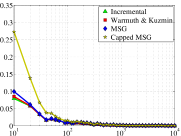
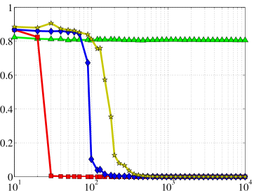
Suboptimality
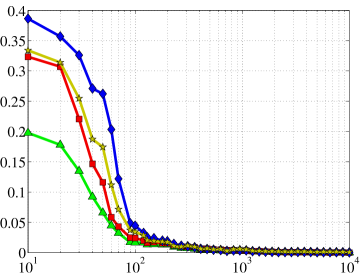
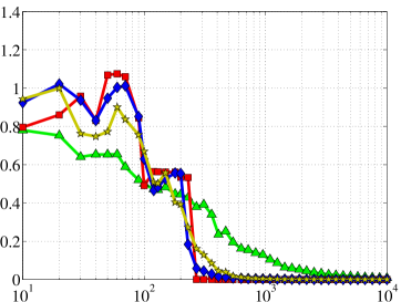
Suboptimality
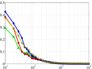
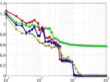
	Iterations	Iterations

Figure 6.3: Plots of suboptimality (vertical axis) versus iteration count (horizontal axis) on simulated data. Each row of plots corresponds to a different choice of the parameter $k$, which is both the subspace dimension sought by the algorithms, and the parameter to the covariance of the data distribution $\Sigma^{(k)}$. The first row has $k=1$, the second $k=2$ and the third $k=4$. In the first column of plots, the data distribution is Gaussian, while in the second column it is the “orthogonal distribution” described in Section 34.1.

	Gaussian	Orthogonal
$k_{t}^{\prime}$
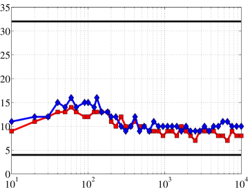
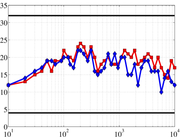
	Iterations	Iterations
Eigenvalue
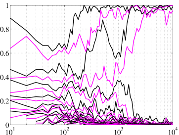
	Iterations	Iterations
Suboptimality
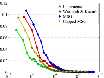
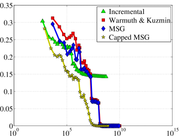
	Est. runtime	Est. runtime

Figure 6.4: In-depth look at simulated-data experiments with $k=4$. First row: the ranks $k_{t}^{\prime}$ of the iterates found by MSG. Middle row: the eigenvalues of the iterates $M^{(t)}$ found by MSG. Bottom row: suboptimality as a function of estimated runtime $\sum_{s=1}^{t}(k_{s}^{\prime})^{2}$. In the first column of plots, the data distribution is Gaussian, while in the second column it is the “orthogonal distribution” described in Section 34.1.

Our first round of experiments is designed to explore both the raw performance of our algorithms (MSG and capped MSG) on distributions which we believe to be particularly bad for them. To this end, we generated data from known $32$-dimensional distributions with diagonal covariance matrices $\Sigma^{(k)}=\mbox{{diag}}(\sigma^{(k)}/\left\lVert{\sigma^{(k)}}\right\rVert)$, where $\sigma$ is the average of a “smooth” portion and a discontinuous portion:

$$\sigma^{(k)}_{i}=\frac{1}{2}\left(\frac{(1.1)^{-i}}{\sum_{j=1}^{32}(1.1)^{-j}}+\frac{\mathbf{1}_{i\leq k}}{k}\right)$$

Observe that $\Sigma^{(k)}$ has a smoothly-decaying set of eigenvalues, except that there is a large gap between the $k$th and $(k+1)$th eigenvalues. We experimented with $k\in\{1,2,4\}$, where $k$ is both the desired subspace dimension used by each algorithm, and also the parameter defining $\Sigma^{(k)}$. Hence, these are examples of relatively “easy” problems for the algorithm of Warmuth and Kuzmin [61], in that the compression loss suffered by the best $k$-dimensional subspace is relatively small. As was mentioned in Section 32, this is the regime in which their upper bound on the convergence rate of their algorithm is superior to that of MSG (Lemma LABEL:lem:pca-capped-msg:rate).

In addition to varying $k$, we also experimented with two different distributions of the same covariance $\Sigma^{(k)}$. The first is simply a Gaussian distribution with covariance matrix $\Sigma^{(k)}$. The second is meant to be particularly hard for algorithms (such as the incremental algorithm of Section 24 and capped MSG algorithm of Section 33) which place a hard cap on the rank of their iterates: the distribution samples the $i$th standard unit basis vector $e_{i}$ with probability $\sqrt{\Sigma_{ii}}$. We refer to this as the “orthogonal distribution”, since it is a discrete distribution over $32$ orthogonal vectors. Interestingly, while this is a “hard” distribution for the incremental and capped MSG algorithms, it is particularly easy for SAA, since, as we saw in Section 22, this algorithm will perform extremely well when $\mathcal{D}$ is supported on $d$ orthogonal directions. The reason for this difference is that the two “capped” algorithms have a type of memory, and will tend to “forget” directions supported on infrequent but large-magnitude samples.

All of the compared algorithms except the incremental algorithm have a step-size parameter. In these experiments, we ran each algorithm for the decreasing step sizes $\eta_{t}=c/\sqrt{t}$ for $c\in 2^{-12:5}$, and created plots for the best choice of $c$, in terms of the average suboptimality over the run (on the real-data experiments of the following section, we use a validation-based approach to choosing the step-size).

Figure 6.3 contains plots of individual runs of MSG, capped MSG with $K=k+1$, the incremental algorithm, and Warmuth and Kuzmin’s algorithm, all based not only on the same sequence of samples drawn from $\mathcal{D}$. On the Gaussian data distribution (top row), all of the algorithms performed roughly comparably, with the incremental algorithm seemingly being the best-performer, followed by Warmuth & Kuzmin’s algorithm. On the orthogonal distribution (bottom row), the behavior of the algorithms changed markedly, with the incremental algorithm getting stuck for $k\in\{1,4\}$, and the others intermittently plateauing at intermediate solutions before beginning to again converge rapidly towards the optimum. This behavior is to be expected on the capped MSG algorithm, due to the fact that the dimension of the subspace stored at each iterate is constrained. However, it is somewhat surprising that MSG and Warmuth & Kuzmin’s algorithm behaved similarly.

In Figure 6.4, we look in greater depth at the results for the orthogonal distribution with $k=4$. We can see from the left-hand plot that both MSG and Warmuth & Kuzmin’s algorithm maintain subspaces of roughly dimension $15$. For reference, the $k_{t}^{\prime}$ for both algorithms tended to be roughly $10$ on the Gaussian distribution with $k=4$ or orthogonal distribution with $k=1$, and roughly $3$ for the Gaussian distribution with $k=1$. The middle plot shows how the set of nonzero eigenvalues of the MSG iterates evolves over time, from which we can see that many of the extra ranks are “wasted” on very small eigenvalues, corresponding to directions which leave the state matrix only a handful of iterations after they enter. This indicates that constraining $k_{t}^{\prime}$, as is done by capped MSG, may indeed be safe, and lead to significant speedups. Indeed, as is shown in the right-hand plot, the low cost-per-iteration of capped MSG causes it to find good solutions using significantly less computation than the others.

34.2   Real Data

Suboptimality
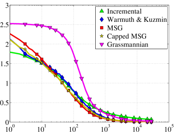
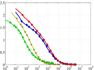
Suboptimality
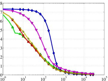
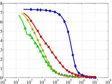
Suboptimality
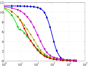
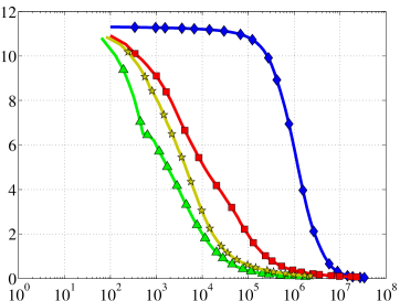
	Iterations	Est. Runtime

Figure 6.5: Plots of suboptimality (vertical axis) versus the iteration count or estimated runtime (horizontal axis) on the MNIST dataset. Each row of plots corresponds to a different choice of the parameter $k$, with the first row having $k=1$, the second $k=4$ and the third $k=8$. The first column of plots shows suboptimality as a function of iteration count, while the second column shows suboptimality as a function of estimated runtime $\sum_{s=1}^{t}(k_{s}^{\prime})^{2}$.

Our second set of experiments measure the performance of various stochastic approximation algorithms for PCA in terms of the population objective, both as a function of number of iterations as well as the estimated computational complexity, which, as in Section 34.1, we compute from the representation size of the internal state maintained by each algorithm. Since we cannot evaluate the true population objective, we estimate it by evaluating on a held-out test set. We use 40% of samples in the dataset for training, 20% for validation, and 40% for testing.

These experiments were performed on the MNIST dataset, which consists of $70,000$ binary images of handwritten digits of size $28\times 28$, resulting in a dimension of $784$. We normalized the data by mean centering the feature vectors and scaling each feature by the product of its standard deviation and the data dimension, so that each feature vector has zero mean and unit norm in expectation. The results are averaged over $100$ random splits into train-validation-test sets. We are interested in learning a maximum variance subspace of dimension $k\in{1,4,8}$ in a single “pass” over the training sample. For all algorithms requiring a step size (e.g. all except incremental), we tried the decreasing sequence of step sizes $\eta_{t}=\frac{c}{\sqrt{t}}$ for each $c\in\{2^{-20},2^{-19},\ldots,2^{6}\}$, chose the $c$ which minimized the average validation suboptimality, and reported the suboptimality experienced for this choice of $c$ on the test set.

Figure 6.5 plots suboptimality as a function of the number of samples processed (iterations), and also as a function of the estimated runtime (computed as in Section 34.1). The incremental algorithm makes the most progress per iteration and is also the fastest of all algorithms. MSG is comparable to the incremental algorithm in terms of the the progress made per iteration. However, its runtime is a worse than the incremental because it will often keep a slightly larger representation (of dimension $k_{t}^{\prime}$) than the incremental algorithm. The capped MSG variant (with $K=k+1$) is significantly faster—almost as fast as the incremental algorithm, while, as we saw in the previous section, being less prone to getting stuck. Warmuth & Kuzmin’s algorithm fares well with $k=1$, but its performance drops for higher $k$. Inspection of the underlying data shows that, in the $k\in\{4,8\}$ experiments, it also tends to have a larger $k_{t}^{\prime}$ than MSG in these experiments, and therefore has a higher cost-per-iteration. GROUSE performs better than Warmuth & Kuzmin’s algorithm, but fares much worse when compared with the MSG and capped MSG.

The most important “message” of these experiments is that the capped MSG algorithm, despite its similarity to the incremental algorithm, has far less of a tendency to get stuck, even when $K=k+1$, while still performing nearly as well even in those cases in which the incremental algorithm converges rapidly. Hence, it is a good “safe” alternative to the incremental algorithm.

Collaborators:

The work presented in this chapter was performed jointly with Raman Arora and Nathan Srebro.

35   Proofs for Chapter 6

lem:pca-capped-msg:rate

Suppose that we perform $T$ iterations of MSG on Problem 6.2, with step size $\eta=2\sqrt{\frac{k}{T}}$. Further suppose WLOG that $\mathbb{E}_{x\sim\mathcal{D}}\left[\left\lVert{x}\right\rVert^{4}\right]\leq 1$. Then:

$$\mathbb{E}_{x\sim\mathcal{D}}\left[x^{T}M^{*}x-x^{T}\bar{M}x\right]\leq 2\sqrt{\frac{k}{T}}$$

where $\bar{M}=\frac{1}{T}\sum_{t=1}^{T}M^{(t)}$ is the average of the iterates, and $M^{*}$ is the optimum (a rank $k$ projection matrix which projects onto the maximal $k$ eigenvectors of the second-moment matrix of $\mathcal{D}$). (Based on Lemma 55 of Sridharan [58], which in turn is based on Nemirovski and Yudin [40]) Define $\tilde{M}^{(t+1)}=M^{(t)}+\eta x_{t}x_{t}^{T}$, and observe that:

$$\eta\left(\sum_{t=1}^{T}x_{t}^{T}M^{*}x_{t}-\sum_{t=1}^{T}x_{t}^{T}M^{(t)}x_{t}\right)$$

$$=\sum_{t=1}^{T}\left\langle{\eta x_{t}x_{t}^{T}},{M^{*}-M^{(t)}}\right\rangle_{F}$$

$$=\frac{1}{2}\sum_{t=1}^{T}\left(\eta^{2}\left\lVert{x_{t}}\right\rVert^{4}+\left\lVert{M^{*}-M^{(t)}}\right\rVert_{F}^{2}-\left\lVert{M^{*}-\tilde{M}^{(t+1)}}\right\rVert_{F}^{2}\right)$$

$$\leq\frac{1}{2}\sum_{t=1}^{T}\left(\eta^{2}\left\lVert{x_{t}}\right\rVert^{4}+\left\lVert{M^{*}-M^{(t)}}\right\rVert_{F}^{2}-\left\lVert{M^{*}-M^{(t+1)}}\right\rVert_{F}^{2}\right)$$

$$\leq\frac{\eta^{2}}{2}\sum_{t=1}^{T}\left\lVert{x_{t}}\right\rVert^{4}+\frac{1}{2}\left\lVert{M^{*}-M^{(1)}}\right\rVert_{F}^{2}$$

Dividing through by $\eta T$, taking expectations (observe that $x_{t}$ and $M^{(t)}$ are conditionally independent), and using the bounds $\mathbb{E}_{x\sim\mathcal{D}}\left[\left\lVert{x}\right\rVert^{4}\right]\leq 1$ and $\left\lVert{M^{*}-M^{(1)}}\right\rVert_{F}^{2}\leq 4k$ ($2\sqrt{k}$ bounds the diameter of the feasible region) gives that:

$$\mathbb{E}_{x\sim\mathcal{D}}\left[xM^{*}x-x\bar{M}x\right]\leq\frac{\eta}{2}+\frac{2k}{\eta T}.$$

Choosing $\eta=2\sqrt{\frac{k}{T}}$ completes the proof. lem:pca-capped-msg:projection

Let $M^{\prime}\in\mathbb{R}^{d\times d}$ be a symmetric matrix, with eigenvalues $\sigma_{1}^{\prime},\dots,\sigma_{d}^{\prime}$ and associated eigenvectors $v_{1}^{\prime},\dots,v_{d}^{\prime}$. If $M=\mathcal{P}\left(M^{\prime}\right)$ projects $M^{\prime}$ onto the feasible region of Problem 6.2 with respect to the Frobenius norm, then $M$ will be the unique feasible matrix which has the same set of eigenvectors as $M^{\prime}$, with the associated eigenvalues $\sigma_{1},\dots,\sigma_{d}$ satisfying:

$$\sigma_{i}=\max\left(0,\min\left(1,\sigma_{i}^{\prime}+S\right)\right)$$

with $S\in\mathbb{R}$ being chosen in such a way that:

$$\sum_{i=1}^{d}\sigma_{i}=k$$

This is the same proof technique as was used to prove Lemma LABEL:lem:pca-warmuth:projection in Chapter 5. We begin by writing the problem of finding $M$ in the form of a convex optimization problem as:

$$\mbox{minimize}: \ \ \left\lVert{M-M^{\prime}}\right\rVert_{F}^{2}$$

$$\mbox{subject to}: \ \ 0\preceq M\preceq I,\operatorname{tr}M=k.$$

Because the objective is strongly convex, and the constraints are convex, this problem must have a unique solution. Letting $\sigma_{1},\dots,\sigma_{d}$ and $v_{1},\dots,v_{d}$ be the eigenvalues and associated eigenvectors of $M$, we may write the KKT first-order optimality conditions [6] as:

$$0=M-M^{\prime}+\mu I-\sum_{i=1}^{d}\alpha_{i}v_{i}v_{i}^{T}+\sum_{i=1}^{d}\beta_{i}v_{i}v_{i}^{T}$$ (6.5)

where $\mu$ is the Lagrange multiplier for the constraint $\operatorname{tr}M=k$, and $\alpha_{i},\beta_{i}\geq 0$ are the Lagrange multipliers for the constraints $0\preceq M$ and $M\preceq I$, respectively. The complementary slackness conditions are that $\alpha_{i}\sigma_{i}=\beta_{i}\left(\sigma_{i}-1\right)=0$. In addition, $M$ must be feasible.

Because every term in Equation 6.5 except for $M^{\prime}$ has the same set of eigenvectors as $M$, it follows that an optimal $M$ must have the same set of eigenvectors as $M^{\prime}$, so we may take $v_{i}=v_{i}^{\prime}$, and write Equation 6.5 purely in terms of the eigenvalues:

$$\sigma_{i}=\sigma_{i}^{\prime}-\mu+\alpha_{i}-\beta_{i}$$

Complementary slackness and feasibility with respect to the constraints $0\preceq M\preceq I$ gives that if $0\leq\sigma_{i}^{\prime}-\mu\leq 1$, then $\sigma_{i}=\sigma_{i}^{\prime}-\mu$. Otherwise, $\alpha_{i}$ and $\beta_{i}$ will be chosen so as to clip $\sigma_{i}$ to the active constraint:

$$\sigma_{i}=\max\left(0,\min\left(1,\sigma_{i}^{\prime}-\mu\right)\right)$$

Primal feasibility with respect to the constraint $\operatorname{tr}M=k$ gives that $\mu$ must be chosen in such a way that $\operatorname{tr}M=k$, completing the proof. lem:pca-capped-msg:capping

Consider the capped-MSG algorithm with $K>k$, and suppose that the true second moment matrix $\Sigma=\mathbb{E}_{x\sim\mathcal{D}}\left[xx^{T}\right]$ has no repeated eigenvalues. Then Problem 6.4, despite not being a convex optimization problem (for $K<d$), has no local optima, and its unique global optimum is the rank-$k$ matrix projecting onto the span of the top-$k$ eigenvectors of $\Sigma$. We’ll prove this by considering two cases: first, that in which $M$ has rank-$k$, and next, that it which it has rank higher than $k$.

Case 1:

suppose that $M$ has exactly $k$ nonzero eigenvalues, but that the corresponding eigenvectors do not span the maximal subspace. Let $v_{1},\dots,v_{k}$ be the eigenvectors of $M$, and observe that, by the assumption that $M$ is not optimal, there must exist a $v_{k+1}$ of norm $1$ which is orthogonal to $v_{1},\dots,v_{k}$ such that the matrix $\tilde{M}$ projecting onto the maximal rank-$k$ subspace in the span of $v_{1},\dots,v_{k+1}$ has strictly larger objective function value that $M$. Both $M$ and $\tilde{M}$ reside in the convex set:

$$\mathcal{S}=\left\{M:VV^{T}M=M\wedge 0\preceq M\preceq I\wedge\operatorname{tr}M=k\right\}$$

Here, $V$ is the matrix containing $v_{1},\dots,v_{k+1}$ in its columns, so that $\mathcal{S}$ is essentially what the feasible region of the convex non-capped MSG objective would be if it were restricted to the span of $v_{1},\dots,v_{k+1}$. Furthermore, $\mathcal{S}$ is a subset of the feasible region of Problem 6.4. Since $M$ is not optimal on this convex subset of the feasible region, it cannot be a local optimum.

Case 2:

Suppose that $M$ has more than $k$ nonzero eigenvalues, and let $i=\operatorname{argmin}_{\sigma_{i}>0}v_{i}^{T}\Sigma v_{i}$. Then, by the same reasoning as was used in Section 27.1 of Chapter 5, we may move a $\sigma_{i}$-sized amount of the mass onto the $\sigma_{j}$s with $\{j:\sigma_{j}>0\wedge j\neq i\}$ without decreasing the objective function value. Furthermore, we may do this continuously. The rank-$k$ solution which we find via this procedure is, by case 1, not a local optimum, and can only be the global optimum if this transfer of mass increases the objective function value, since $\Sigma$ has no repeated eigenvalues. Hence, $M$ itself is not a local optimum, but is at worst a saddle point.

References

- Arora et al. [2012] Raman Arora, Andrew Cotter, Karen Livescu, and Nathan Srebro. Stochastic optimization for pca and pls. In 50th Annual Allerton Conference on Communication, Control, and Computing, 2012.
- Balzano et al. [2010] Laura Balzano, Robert Nowak, and Benjamin Recht. Online identification and tracking of subspaces from highly incomplete information. CoRR, abs/1006.4046, 2010.
- Bartlett and Mendelson [2003] Peter L. Bartlett and Shahar Mendelson. Rademacher and Gaussian complexities: risk bounds and structural results. JMLR, 3:463–482, Mar 2003.
- Blum et al. [1973] M. Blum, R. W. Floyd, V. Pratt, R. L. Rivest, and R. E. Tarjan. Time bounds for selection. JCSS, 7(4):448–461, August 1973.
- Bottou and Bousquet [2008] L. Bottou and O. Bousquet. The tradeoffs of large scale learning. In NIPS’07, pages 161–168, 2008.
- Boyd and Vandenberghe [2004] Stephen Boyd and Lieven Vandenberghe. Convex Optimization. Cambridge University Press, 2004.
- Brin and Page [1998] Sergey Brin and Larry Page. The anatomy of a large-scale hypertextual web search engine. In Proceedings of the 7th international conference on World Wide Web (WWW), pages 107–117, 1998.
- Burges and Schölkopf [1997] C. Burges and B. Schölkopf. Improving the accuracy and speed of support vector machines. In NIPS’97, pages 375–381. MIT Press, 1997.
- C. Cortes [1995] V. Vapnik C. Cortes. Support -vector networks. Machine Learning, 20(3):273–297, 1995.
- Cavallanti et al. [2007] G. Cavallanti, N. Cesa-Bianchi, and C. Gentile. Tracking the best hyperplane with a simple budget perceptron. Machine Learning, 69(2-3), December 2007.
- Cesa-Bianchi et al. [2001] N. Cesa-Bianchi, A. Conconi, and C. Gentile. On the generalization ability of on-line learning algorithms. IEEE Trans. on Inf. Theory, 50:2050–2057, 2001.
- Chang and Lin [2001] C-C. Chang and C-J. Lin. LIBSVM: a library for support vector machines, 2001. Software available at http://www.csie.ntu.edu.tw/~cjlin/libsvm.
- Chen et al. [2006] P-H. Chen, R-E. Fan, and C-J. Lin. A study on smo-type decomposition methods for support vector machines. IEEE Transactions on Neural Networks, 17(4):893–908, 2006.
- Collins et al. [2008] M. Collins, A. Globerson, T. Koo, X. Carreras, and P. Bartlett. Exponentiated gradient algorithms for conditional random fields and max-margin markov networks. JMLR, 9:1775–1822, 2008.
- Collobert et al. [2006] Ronan Collobert, Fabian Sinz, Jason Weston, and Léon Bottou. Trading convexity for scalability. In ICML’06, pages 201–208, 2006.
- Coppersmith and Winograd [1990] Don Coppersmith and Shmuel Winograd. Matrix multiplication via arithmetic progressions. 9(3):251–280, 1990.
- Cotter et al. [2011] A. Cotter, N. Srebro, and J. Keshet. A GPU-tailored approach for training kernelized SVMs. In KDD’11, 2011.
- Cotter et al. [2012] A. Cotter, S. Shalev-Shwartz, and N. Srebro. The kernelized stochastic batch perceptron. In ICML’12, 2012.
- Cotter et al. [2013] A. Cotter, S. Shalev-Shwartz, and N. Srebro. Learning optimally sparse support vector machines. In ICML’13, 2013.
- Dekel et al. [2005] O. Dekel, S. Shalev-Shwartz, and Y. Singer. The forgetron: A kernel-based perceptron on a fixed budget. In NIPS’05, pages 259–266, 2005.
- Fan et al. [2005] R-E. Fan, P-S. Chen, and C-J. Lin. Working set selection using second order information for training support vector machines. JMLR, 6:1889–1918, 2005.
- Freund and Schapire [1999] Y. Freund and R. E. Schapire. Large margin classification using the perceptron algorithm. Machine Learning, 37(3):277–296, 1999.
- Gu [2000] M. Gu. Single- and multiple-vector iterations. In Bai, Zhaojun, Demmel, James, Dongarra, Jack, Ruhe, Axel, and van der Vorst, Henk, editors, Templates for the solution of algebraic eigenvalue problems: a practical guide, chapter 4.3. Society for Industrial and Applied Mathematics, Philadelphia, PA, 2000.
- Hayashi [2006] Masahito Hayashi. Quantum Information: An Introduction. Springer, 2006. ISBN 9783540302650.
- Hazan et al. [2011] E. Hazan, T. Koren, and N. Srebro. Beating SGD: Learning SVMs in sublinear time. In NIPS’11, 2011.
- Hiai et al. [1981] Fumio Hiai, Masanori Ohya, and Makoto Tsukada. Sufficiency, KMS conditions and relative entropy in von Neumann algebras. Pacific Journal of Mathematics, 96(1), 1981.
- Hsieh et al. [2008] C-J. Hsieh, K-W. Chang, C-J. Lin, S. S. Keerthi, and S. Sundararajan. A dual coordinate descent method for large-scale linear SVM. In ICML’08, pages 408–415, 2008.
- Hush et al. [2006] D. Hush, P. Kelly, C. Scovel, and I. Steinwart. QP algorithms with guaranteed accuracy and run time for support vector machines. JMLR, 7:733–769, 2006.
- Joachims and Yu [2009] T. Joachims and Chun-Nam Yu. Sparse kernel svms via cutting-plane training. Machine Learning, 76(2–3):179–193, 2009. European Conference on Machine Learning (ECML) Special Issue.
- Kakade and Tewari [2009] Sham M. Kakade and Ambuj Tewari. On the generalization ability of online strongly convex programming algorithms. In NIPS’09, 2009.
- Kakade et al. [2008] Sham M. Kakade, Karthik Sridharan, and Ambuj Tewari. On the complexity of linear prediction: Risk bounds, margin bounds and regularization. In NIPS’08, 2008.
- Kakade et al. [2012] Sham M. Kakade, Shai Shalev-Shwartz, and Ambuj Tewari. Regularization techniques for learning with matrices. Journal of Machine Learning Research, 13:1865–1890, 2012.
- Keerthi et al. [2006] S. Sathiya Keerthi, Olivier Chapelle, and Dennis DeCoste. Building support vector machines with reduced classifier complexity. Journal of Machine Learning Research, 7:1493–1515, 2006.
- Kim et al. [2005] Kwang In Kim, Matthias O. Franz, and Bernhard Schölkopf. Iterative kernel principal component analysis for image modeling. IEEE Trans. PAMI, 27(9):1351–1366, 2005.
- Kuzmin and Warmuth [2007] Dima Kuzmin and Manfred K. Warmuth. Online kernel PCA with entropic matrix updates. In ICML’07, 2007.
- Lee and Mangasarian [2001] Y-J. Lee and O. Mangasarian. RSVM: Reduced support vector machines. In Data Mining Institute, Computer Sciences Department, University of Wisconsin, pages 00–07, 2001.
- Lin and Lin [2003] K-M. Lin and C-J. Lin. A study on reduced support vector machines. IEEE Transactions on Neural Networks, 2003.
- Melville [1851] Herman Melville. Moby-Dick. Harper & Brothers, 1851.
- Nemirovski et al. [2009] A. Nemirovski, A. Juditsky, G. Lan, and A. Shapiro. Robust stochastic approximation approach to stochastic programming. SIAM Journal on Optimization, 19(4):1574–1609, January 2009.
- Nemirovski and Yudin [1983] Arkadi Nemirovski and David Yudin. Problem complexity and method efficiency in optimization. John Wiley & Sons Ltd, 1983.
- Nesterov [2009] Y. Nesterov. Primal-dual subgradient methods for convex problems. Math. Program., 120(1):221–259, Apr 2009.
- Nguyen et al. [2010] D D. Nguyen, K. Matsumoto, Y. Takishima, and K. Hashimoto. Condensed vector machines: learning fast machine for large data. Trans. Neur. Netw., 21(12):1903–1914, Dec 2010.
- Nocedal and Wright [1999] Jorge Nocedal and Stephen J. Wright. Numerical Optimization. Springer, New York, 1999.
- Oja and Karhunen [1985] Erkki Oja and Juha Karhunen. On stochastic approximation of the eigenvectors and eigenvalues of the expectation of a random matrix. Journal of Mathematical Analysis and Applications, 106:69–84, 1985.
- Osuna and Girosi [1998] E. Osuna and F. Girosi. Reducing the run-time complexity of support vector machines, 1998.
- Platt [1998] J. C. Platt. Fast training of support vector machines using Sequential Minimal Optimization. In B. Schölkopf, C. Burges, and A. J. Smola, editors, Advances in Kernel Methods - Support Vector Learning. MIT Press, 1998.
- Rahimi and Recht [2007] A. Rahimi and B. Recht. Random features for large-scale kernel machines. In NIPS’07, 2007.
- Sanger [1989] Terence D. Sanger. Optimal unsupervised learning in a single-layer linear feedforward neural network. Neural Networks, 12:459–473, 1989.
- Shalev-Shwartz [2007] S. Shalev-Shwartz. Online Learning: Theory, Algorithms, and Applications. PhD thesis, The Hebrew University of Jerusalem, July 2007.
- Shalev-Shwartz [2010] S. Shalev-Shwartz. Introduction to machine learning, lecture notes. Technical report, The Hebrew University, 2010. http://www.cs.huji.ac.il/~shais/Handouts2010.pdf.
- Shalev-Shwartz and Srebro [2008] S. Shalev-Shwartz and N. Srebro. SVM optimization: Inverse dependence on training set size. In ICML’08, pages 928–935, 2008.
- Shalev-Shwartz and Zhang [2013] S. Shalev-Shwartz and T. Zhang. Stochastic dual coordinate ascent methods for regularized loss minimization. JMLR, 14:567–599, February 2013.
- Shalev-Shwartz et al. [2007] S. Shalev-Shwartz, Y. Singer, and N. Srebro. Pegasos: Primal Estimated sub-GrAdient SOlver for SVM. In ICML’07, pages 807–814, 2007.
- Shalev-Shwartz et al. [2011] S. Shalev-Shwartz, Y. Singer, N. Srebro, and A. Cotter. Pegasos: Primal Estimated sub-GrAdient SOlver for SVM. Mathematical Programming, 127(1):3–30, March 2011.
- Shalev-Shwartz and Tewari [2009] Shai Shalev-Shwartz and Ambuj Tewari. Stochastic methods for l1 regularized loss minimization. In Proceedings of the 26th Annual International Conference on Machine Learning, ICML’09, pages 929–936, New York, NY, USA, 2009. ACM.
- Srebro et al. [2010] N. Srebro, K. Sridharan, and A. Tewari. Smoothness, low-noise and fast rates. In NIPS’10, 2010.
- Srebro et al. [2011] Nathan Srebro, Karthik Sridharan, and Ambuj Tewari. On the universality of online mirror descent. In NIPS’11, 2011.
- Sridharan [2011] Karthik Sridharan. Learning From An Optimization Viewpoint. PhD thesis, Toyota Technological Institute at Chicago, 2011.
- Strassen [1969] Volker Strassen. Gaussian elimination is not optimal. 13(4):354–356, august 1969.
- Warmuth and Kuzmin [2006] Manfred K. Warmuth and Dima Kuzmin. Randomized PCA algorithms with regret bounds that are logarithmic in the dimension. In NIPS’06, 2006.
- Warmuth and Kuzmin [2008] Manfred K. Warmuth and Dima Kuzmin. Randomized online PCA algorithms with regret bounds that are logarithmic in the dimension. Journal of Machine Learning Research (JMLR), 9:2287–2320, 2008.
- Wikipedia [2013] Wikipedia. Matrix multiplication — Wikipedia, the free encyclopedia, May 2013. [Online; accessed 30-May-2013].
- Wu et al. [2005] M. Wu, B. Schölkopf, and G. Bakir. Building sparse large margin classifiers. In ICML’05, pages 996–1003, New York, NY, USA, 8 2005. Max-Planck-Gesellschaft, ACM.
- Zhan and Shen [2005] Y. Zhan and D. Shen. Design efficient support vector machine for fast classification. Pattern Recognition, 38(1):157–161, 2005.
- Zhang [2004] T. Zhang. Solving large scale linear prediction problems using stochastic gradient descent algorithms. In ICML’04, 2004.
- Zinkevich [2003] M. Zinkevich. Online convex programming and generalized infinitesimal gradient ascent. In ICML’03, 2003.