Random Walks on Directed Networks: Inference and Respondent-driven Sampling

Abstract

Respondent driven sampling (RDS) is a method often used to estimate population properties (e.g. sexual risk behavior) in hard-to-reach populations. It combines an effective modified snowball sampling methodology with an estimation procedure that yields unbiased population estimates under the assumption that the sampling process behaves like a random walk on the social network of the population. Current RDS estimation methodology assumes that the social network is undirected, i.e. that all edges are reciprocal. However, empirical social networks in general also have non-reciprocated edges. To account for this fact, we develop a new estimation method for RDS in the presence of directed edges on the basis of random walks on directed networks. We distinguish directed and undirected edges and consider the possibility that the random walk returns to its current position in two steps through an undirected edge. We derive estimators of the selection probabilities of individuals as a function of the number of outgoing edges of sampled individuals. We evaluate the performance of the proposed estimators on artificial and empirical networks to show that they generally perform better than existing methods. This is in particular the case when the fraction of directed edges in the network is large.
Key words: Hidden population; Social network; Renewal process; Estimated degree; Network model.

1 INTRODUCTION

Random walks on networks are crucial to the understanding of many network processes, and in many applications, random walks serve as either rigorous or approximate tools depending on the amount of information available about networks. A network sampling methodology taking advantage of a random walk approximation is respondent-driven sampling (RDS). The method, first suggested in Heckathorn, (1997), is especially suitable for investigating hidden or hard-to-reach populations, such as injecting drug users (IDUs), sex workers, and men who have sex with men (MSM). For such populations, sampling frames are typically unavailable because individuals often suffer from social stigmatization and/or legal difficulties, and conventional sampling methods therefore fail. High demand for valid inference on hidden populations, e.g. on the risk behavior of individuals and the disease prevalence in the population, as well as a lack of competing methods, has made RDS a leading method. Examples of RDS studies from 2013 include MSM in Nanjing, China (Tang et al.,, 2013), undocumented Central American immigrants in Houston, Texas (Montealegre et al.,, 2013), and IDUs in the District of Columbia (Magnus et al.,, 2013).

At the core of RDS is the notion of a social network that binds the population together. During the sampling process, already sampled individuals use their social relations (edges of the social network) to recruit new individuals in the population into the sample, creating a snowball-like mechanism. Additionally, information on the structure of the network collected during the sampling process facilitates unbiased population estimates given that the actual RDS recruitment process behaves like a random walk on the network (Salganik and Heckathorn,, 2004; Volz and Heckathorn,, 2008).

In recent years, much RDS research has focused on the sensitivity of current RDS estimators to violations of the assumptions underlying the estimating process. In fact, it has been shown that RDS estimators may be subject to substantial biases and large variances when some assumptions are not valid (Gile and Handcock,, 2010; Lu et al.,, 2012; Wejnert,, 2009; Tomas and Gile,, 2011; Goel and Salganik,, 2010). New RDS estimators have been developed to mitigate this problem (Gile and Handcock,, 2011; Gile,, 2011; Lu et al.,, 2013).

Current RDS estimation assumes that the social network of the population is undirected. However, real social networks are at least partially directed in general. The directedness of a network can be quantified by the the ratio of the number of non-reciprocal (i.e., directed) edges to the total number of edges in the network (Wasserman and Faust,, 1994). This value lies between 0 and 1, and a large value indicates that the network is close to a purely directed network. Examples of real social networks and social networks, including e-mail social networks, from online communities having a considerable fraction of non-reciprocal edges are shown in Table 1. For these and other directed social networks, RDS methods assuming an undirected network may be biased.

Table 1: Proportion of directed edges in social networks.

Real social networks		Online social networks
High-tech managers	0.71	Google+ (Oct 2011)	0.62
(Wasserman and Faust,, 1994)		(Gong et al.,, 2013)
Dining partners	0.76	Flickr (May 2007)	0.55
(Moreno et al.,, 1960)		(Gong et al.,, 2013)
Radio amateurs	0.59	LiveJournal (Dec 2006)	0.26
(Killworth and Bernard,, 1976)		(Mislove et al.,, 2007)
		Twitter (June 2009)	0.78
		(Kwak et al.,, 2010)
		University e-mail	0.77
		(Newman et al.,, 2002)
		Enron e-mail	0.85
		(Boldi and Vigna,, 2004)
		(Boldi et al.,, 2011)

Motivated by these data, we aim to expand RDS estimation to the case of directed networks. Because the RDS method uses the random walk, a random walk framework for directed networks is a key component to this expansion. This is not a trivial task because the random walk behaves very differently in undirected and directed networks. In particular, the stationary distribution of the random walk is simply proportional to the degree of the vertex in undirected networks (Doyle and Snell,, 1984; Lovász,, 1993), whereas it is affected by the entire network structure in directed networks (Donato et al.,, 2004; Langville and Meyer,, 2006; Masuda and Ohtsuki,, 2009).

In this paper, we first present the commonly available RDS estimation procedures and the basics of random walks on networks in Sections 2 and 3, respectively. Then, we present methods for estimating the stationary distribution from random walks on directed networks and its application to RDS estimation in Section 4. These methods are then evaluated and compared to existing methods by numerical simulations, which we describe in Section 5. The results from simulations are presented in Section 6. Finally, our findings are discussed in Section 7.

2 RESPONDENT-DRIVEN SAMPLING

In practice, an RDS study begins with the selection of a seed group of individuals from the population. Each seed is given a fixed number of coupons, typically three to five, which are effectively the tickets for participation in the study, to be distributed to other peers in the population. Those who have received a coupon and joined the study (i.e., respondents) are also given coupons to be distributed to other peers that have not obtained a coupon. This procedure is repeated until the desired sample size has been reached. Each respondent is rewarded both for participating in the study and for the participation of those to whom he/she passed coupons, resulting in double incentives for participation. The sampling procedure ensures that the identities of members of the population are not revealed in the recruitment process. For each respondent, the properties of interest (e.g., HIV status), number of neighbors (degree), and the neighbors that the respondent has successfully recruited are recorded.

We approximate the RDS recruitment process by a random walk on the social network. To this end, we assume that (i) respondents recruit peers from their social contacts with uniform probability, (ii) each recruitment consists of only one peer, (iii) sampling is done with replacement, such that a respondent may appear in the sample multiple times, (iv) the degree of respondents is accurately reported, and (v) the population forms a connected network. Then, if the random walk is in equilibrium with a known stationary distribution $\{\pi_{i};i=1,\dots,N\}$, where $N$ is the population size, we may estimate $p_{A}$, the fraction of individuals with a property of interest $A$, as (Thompson,, 2012)

$$\hat{p}_{A}=\frac{\sum_{i\in S\cap A}1/\pi_{i}}{\sum_{i\in S}1/\pi_{i}},$$ (1)

where $S$ is our sample. For undirected networks, the stationary distribution is proportional to the degree (Doyle and Snell,, 1984; Lovász,, 1993), and Eq. (1) yields the most widely used RDS estimator (Volz and Heckathorn,, 2008) given by

$$\hat{p}_{A}^{\rm{VH}}=\frac{\sum_{i\in S\cap A}1/d_{i}}{\sum_{i\in S}1/d_{i}},$$ (2)

where $d_{i}$ is the degree of node $i$. However, the estimator given by Eq. (2) may be biased for directed networks (Lu et al.,, 2012, 2013). Therefore, to estimate $p_{A}$ without bias from an RDS sample on a directed network, we need to accurately calculate Eq. (1). Because the stationary distribution $\{\pi_{i}\}$ used in Eq. (1) is analytically intractable for most directed networks, we will proceed by deriving estimators of it.

3 RANDOM WALKS ON DIRECTED NETWORKS

We consider a directed, unweighted, aperiodic, and strongly connected network $G$ with $N$ vertices. Let $e_{ij}=1$ if there is a directed edge from $i$ to $j$ and 0 otherwise. An undirected edge exists between $i$ and $j$ if and only if $e_{ij}=e_{ji}=1$. We denote the number of undirected, in-directed, and out-directed edges at vertex $i$ by $d_{i}^{\rm{(un)}}$, $d_{i}^{\rm{(in)}}$, and $d_{i}^{\rm{(out)}}$, respectively. We use $D^{\rm{(un)}}$, $D^{\rm{(in)}}$, and $D^{\rm{(out)}}$ to refer to the corresponding random variables if a node is drawn uniformly at random. If we specifically mention that the network is undirected, we obtain $d_{i}^{\rm{(in)}}=d_{i}^{\rm{(out)}}=0$, and the degree of vertex $i$ refers to $d_{i}^{\rm{(un)}}=d_{i}$. Otherwise, the degree of vertex $i$ refers to the triplet $(d_{i}^{\rm{(un)}},d_{i}^{\rm{(in)}},d_{i}^{\rm{(out)}})$. We refer to $d_{i}^{\rm{(un)}}+d_{i}^{\rm{(in)}}$ and $d_{i}^{\rm{(un)}}+d_{i}^{\rm{(out)}}$ as the in-degree and out-degree of vertex $i$, respectively. It should be noted that we may observe for example the out-degree $d_{i}^{\rm{(un)}}+d_{i}^{\rm{(out)}}$, but not separately the $d_{i}^{\rm{(un)}}$ and $d_{i}^{\rm{(out)}}$ values.

Consider the simple random walk $\bm{X}=\{X(t);t=0,1,\ldots\}$ with state space $\bm{S}=\{1,\dots,N\}$ on $G$ such that the walker staying at vertex $i$ moves to any of the $d_{i}^{\rm{(un)}}+d_{i}^{\rm{(out)}}$ neighbors reached by an undirected or out-directed edge with equal probability. We denote the stationary distribution of $\bm{X}$ by $\{\pi_{i};i=1,\ldots,N\}$, where $\pi_{i}=\lim_{t\to\infty}P(X(t)=i)$. If we sample from the random walk in equilibrium, vertices will be selected with probabilities given by the stationary distribution, and we then refer to $\{\pi_{i}\}$ as the selection probabilities of the vertices in $G$.

For an arbitrary network, we obtain

$$\pi_{i}=\sum_{j=1}^{N}\frac{e_{ji}}{\sum_{\ell=1}^{N}e_{j\ell}}\pi_{j}=\sum_{j=1}^{N}\frac{e_{ji}}{d_{j}^{\rm{(un)}}+d_{j}^{\rm{(out)}}}\pi_{j},$$ (3)

where the stationary distribution is fully defined by $\sum_{i=1}^{N}\pi_{i}=1$. In undirected networks, we obtain $\pi_{i}=d_{i}/\sum_{j=1}^{N}d_{j}$. In contrast, there is no analytical closed form solution for $\{\pi_{i}\}$ in directed networks. If a directed network has little assortativity (i.e., degree correlation between adjacent vertices), $\{\pi_{i}\}$ is often accurately estimated by the normalized in-degree (Lu et al.,, 2013; Fortunato et al.,, 2008; Ghoshal and Barabási,, 2011) because

$$\pi_{i}\approx\sum_{j=1}^{N}\frac{e_{ji}}{d_{j}^{\rm{(un)}}+d_{j}^{\rm{(out)}}}\bar{\pi}\propto\sum_{j=1}^{N}e_{ji}=d_{i}^{\rm{(in)}}+d_{i}^{\rm{(un)}},$$ (4)

where $\bar{\pi}$ is the average selection probability. However, the estimate given by (4) is often inaccurate in general directed networks (Donato et al.,, 2004; Masuda and Ohtsuki,, 2009). Moreover, since it is much easier for individuals to assess how many people they know (i.e., out-degree) than by how many people they are known (i.e., in-degree), it is common to observe only the out-degree. In this case, Eq. (4) can not be used with an RDS sample.

4 ESTIMATION OF SELECTION PROBABILITIES FOR DIRECTED NETWORKS

We now derive estimators of the selection probabilities for the random walk on directed networks. We first derive an estimation scheme when the full degree $(d_{i}^{\rm{(un)}},d_{i}^{\rm{(in)}},d_{i}^{\rm{(out)}})$ is observed for all the vertices $i$ visited by the random walk. Then, we extend this estimation to the situation in which only the out-degree $d_{i}^{\rm{un}}+d_{i}^{\rm{out}}$ of the visited vertices is observed.

4.1 Estimating Selection Probabilities From Full Degrees

In order to estimate $\{\pi_{i}\}$, we assume that $X(t_{0})=i$ and that $t_{0}$ is sufficiently large for the stationary distribution to be reached. We evaluate the frequency with which $\bm{X}$ visits $i$ in the subsequent times. If $\bm{X}$ leaves $i$ through an undirected edge $e_{i\cdot}^{\rm{(un)}}$, where $e_{i\cdot}^{\rm{(un)}}$ is one of the $d_{i}^{\rm{(un)}}$ undirected edges owned by $i$, $\bm{X}$ may return to $i$ after two steps using the same edge and repeat the same type of returns $m$ times in total, perhaps using different undirected edges $e_{i\cdot}^{\rm{(un)}}$. Then, $X(t_{0})=X(t_{0}+2)=\cdots=X(t_{0}+2m)=i$ and $X(t_{0}+2m+2)=k$ for some $k\neq i$.

If $X(t_{0}+2)=i$, the walk first moves from $i$ through an undirected edge to vertex $j$ at $t=t_{0}+1$ and returns to $i$ through the same edge at $t=t_{0}+2$. The probability of this event is given by $d_{i}^{\rm{(un)}}/(d_{i}^{\rm{(un)}}+d_{i}^{\rm{(out)}})\cdot 1/(d_{j}^{\rm{(un)}}+d_{j}^{\rm{(out)}})$. Because the out-degree of vertex $j$, i.e., $d_{j}^{\rm{(un)}}+d_{j}^{\rm{(out)}}$, is unknown, we approximate $1/(d_{j}^{\rm{(un)}}+d_{j}^{\rm{(out)}})$ by $E\left(1/(\tilde{D}^{\rm{(un)}}+D^{\rm{(out)}})\right)$. Here $\tilde{D}^{\rm{(un)}}$ denotes the undirected degree distribution under the condition that the vertex is reached by following an undirected edge, i.e. a size-biased distribution for the undirected degree, $P(\tilde{D}^{\rm{(un)}}=d)\propto dP(D^{\rm{(un)}}=d)$ (Newman,, 2010). It is also possible to estimate $1/(d_{j}^{\rm{(un)}}+d_{j}^{\rm{(out)}})$ by $1/E(\tilde{D}^{\rm{(un)}}+D^{\rm{(out)}})$, which however showed to have hardly any effect in our simulations, and if any, slightly worse. Thus, we estimate the probability of returning to vertex $i$ after two steps by

$$p_{i}^{\rm{(ret)}}=\frac{d_{i}^{\rm{(un)}}}{d_{i}^{\rm{(un)}}+d_{i}^{\rm{(out)}}}E\left(\frac{1}{\tilde{D}^{\rm{(un)}}+D^{\rm{(out)}}}\right).$$ (5)

When $t\geq t_{0}+2m+3$, we use Eq. (4) to estimate the probability to visit vertex $i$ at any time as being proportional to $d_{i}^{\rm{(un)}}+d_{i}^{\rm{(in)}}$, i.e.,

$$p_{i}^{\rm{(vis)}}=\frac{d_{i}^{\rm{(un)}}+d_{i}^{\rm{(in)}}}{N(E(D^{\rm{(un)}})+E(D^{\rm{(in)}}))}.$$ (6)

Under these estimates, the number of returns after two steps to vertex $i$, counting the starting point $X(t_{0})=i$ as a return to $i$, is geometrically distributed with expected value $1/(1-p_{i}^{\rm{(ret)}})$, and the number of steps starting from $t=t_{0}+2m+2$, counting this step, and ending at the time immediately before visiting $i$ with probability $p_{i}^{\rm{(vis)}}$ is geometrically distributed with expected value $1/p_{i}^{\rm{(vis)}}$.

(a) $Z_{i}^{n}$ consecutive returns to $i$.

(b) Leaves $i$ for $Y_{i}^{n}$ steps.

Figure 1: Schematic of a renewal period. a) The walker makes $Z_{i}^{n}$ consecutive direct returns to $i$. b) The walker leaves $i$ without an immediate return, because the walker leaves $i$ by a directed edge or leaves $j$ by another edge. Then, the walker returns to $i$ after $Y_{i}^{n}$ steps.

We then have a renewal process $\{R_{i}^{n};n\geq 1,R_{i}^{0}=0\}$ with the $n$th renewal occurring at random time $R_{i}^{n}=\sum_{k=1}^{n}(2Z_{i}^{k}+Y_{i}^{k})$, where $Z_{i}^{n}\sim Ge(1-p_{i}^{\rm{(ret)}})$ and $Y_{i}^{n}\sim Ge(p_{i}^{\rm{(vis)}})$. In Figure 1, the behavior of the process during a renewal period is schematically shown. The average time step between consecutive renewal events is equal to $2E(Z_{i}^{n})+E(Y_{i}^{n})$. The average number of visits to $i$ between the two renewal events, with the visit to $i$ at $t=t_{0}$ included, is equal to $E(Z_{i}^{n})$. Therefore, from renewal theory (see e.g., Resnick,, 1992), we obtain an estimate of $\pi_{i}$ as

$$\pi_{i}\approx\frac{E(Z_{i}^{n})}{2E(Z_{i}^{n})+E(Y_{i}^{n})}=\frac{\frac{1}{1-p_{i}^{\rm{(ret)}}}}{2\frac{1}{1-p_{i}^{\rm{(ret)}}}+\frac{1}{p_{i}^{\rm{(vis)}}}}=\frac{p_{i}^{\rm{(vis)}}}{2p_{i}^{\rm{(vis)}}+1-p_{i}^{\rm{(ret)}}}.$$ (7)

Because $p_{i}^{\rm{(ret)}}=O(1)$ and $p_{i}^{\rm{(vis)}}=O(1/N)$, removing higher order terms in Eq. (7) yields

$$\hat{\pi}_{i}\approx\frac{p_{i}^{\rm{(vis)}}}{1-p_{i}^{\rm{(ret)}}}\propto\frac{d_{i}^{\rm{(un)}}+d_{i}^{\rm{(in)}}}{1-\frac{d_{i}^{\rm{(un)}}}{d_{i}^{\rm{(un)}}+d_{i}^{\rm{(out)}}}E\left(\frac{1}{\tilde{D}^{\rm{(un)}}+D^{\rm{(out)}}}\right)}.$$ (8)

The proportionality constant is given by imposing that $\sum_{i=1}^{N}\hat{\pi}_{i}=1$. If the network is undirected, we obtain $\hat{\pi}_{i}\propto d_{i}^{\rm{(un)}}$, such that $\hat{\pi}_{i}$ coincides with the exact solution used in Eq. (2). If the network is fully directed, i.e., there are no reciprocal edges and $\alpha=1$, the estimator is proportional to in-directed degree $d_{i}^{\rm{(in)}}$.

4.2 Estimating Selection Probabilities From Out-degrees

A common situation in RDS is that only the out-degrees (i.e., $d_{i}^{\rm{(un)}}+d_{i}^{\rm{(out)}}$) of respondents are recorded. Then, the estimator of the selection probabilities given by Eq. (8) can not be directly used. To cope with this situation, we estimate the number of undirected, in-directed, and out-directed edges from the observed out-degrees and substitute the estimators $(\hat{d}^{\rm{(un)}}_{i},\hat{d}^{\rm{(in)}}_{i},\hat{d}^{\rm{(out)}}_{i})$ in Eq. (8).

Assume that we have observed the out-degree $d_{i}^{\rm{(un)}}+d_{i}^{\rm{(out)}}$ of vertex $i$. We estimate $d^{\rm{(un)}}_{i}$ and $d^{\rm{(out)}}_{i}$ by their expected proportions of the out-degree, and the in-directed degree by its expectation, as follows:

$$\left\{\begin{array}[]{rcl}\hat{d}^{\rm{(un)}}_{i}&=&\frac{E(D^{\rm{(un)}})}{E(D^{\rm{(un)}})+E(D^{\rm{(out)}})}\left(d_{i}^{\rm{(un)}}+d_{i}^{\rm{(out)}}\right),\\ \hat{d}^{\rm{(out)}}_{i}&=&\frac{E(D^{\rm{(out)}})}{E(D^{\rm{(un)}})+E(D^{\rm{(out)}})}\left(d_{i}^{\rm{(un)}}+d_{i}^{\rm{(out)}}\right),\\ \hat{d}_{i}^{\rm{(in)}}&=&E(D^{\rm{(in)}}).\end{array}\right.$$ (9)

The expectations used in Eq. (9) rely on the assumption that we have a random sample from the network, which is not true in this case. A plausible assumption on the sampled degree distributions is that they are size-biased. However, our numerical results suggest that a size-biased distribution for un-directed and/or the in-directed degree makes little difference, and if any, increases the bias of selection probability estimators. Therefore, we stay with the estimators given by Eq. (9).

When $(\hat{d}^{\rm{(un)}}_{i},\hat{d}^{\rm{(in)}}_{i},\hat{d}^{\rm{(out)}}_{i})$ is substituted in Eq. (8) in place of $(d^{\rm{(un)}}_{i},d^{\rm{(in)}}_{i},d^{\rm{(out)}}_{i})$, $\hat{d}_{i}^{\rm{(un)}}/(\hat{d}_{i}^{\rm{(un)}}+\hat{d}_{i}^{\rm{(out)}})$ in the denominator is a constant. Therefore, the estimator is proportional to $\hat{d}^{\rm{(un)}}_{i}+\hat{d}^{\rm{(in)}}_{i}$, i.e., equivalent to Eq. (4) calculated with the estimated degrees.

4.3 Estimating Network Parameters

The estimators of directed degrees in Eq. (9) rely on knowing $E(D^{\rm{(un)}})$, $E(D^{\rm{(in)}})$, and $E(D^{\rm{(un)}})$ separately, which are not estimable from a typical RDS sample, where only the out-degrees $d_{i}^{\rm{(un)}}+d_{i}^{\rm{(out)}}$ of respondents are recorded. Therefore, we need to extend the estimation procedure to handle these unknown moments. We do so by assuming a model for the network from which we can estimate the required moments.

Specifically, we assume that the observed network is a realization of a directed equivalent of the simple $G(N,p=\lambda/(N-1))$ random graph (Erdős and Renyi,, 1960). Given parameters $\alpha\in[0,1]$ and $\lambda\in[0,N-1]$, each pair of vertices independently forms an edge with probability $\lambda/(N-1)$, which is undirected with probability $(1-\alpha)$ and directed with probability $\alpha$. When the edge is directed, the direction is selected with equal probability. It follows that $\lambda$ is the expected total degree of a vertex and that $\alpha$ is the fraction of directed edges as $N\rightarrow\infty$.

If $N$ is large, $D^{\rm{(un)}}$, $D^{\rm{(in)}}$, and $D^{\rm{(out)}}$ approximately follow independent Poisson distributions with parameters $(1-\alpha)\lambda$, $\alpha\lambda/2$, and $\alpha\lambda/2$, respectively. Therefore, the out-degree $D^{\rm{(un)}}+D^{\rm{(out)}}$ and the in-degree $D^{\rm{(un)}}+D^{\rm{(in)}}$ are both Poisson distributed with parameter $(2-\alpha)\lambda/2$. Consequently, if we estimate $\alpha$ and $\lambda$, we can estimate the unknown moments by substituting the estimated $\hat{\alpha}$ and $\hat{\lambda}$ in the moments of the (Poissonian) degree distributions.

To find estimators of $\alpha$ and $\lambda$, we again consider the random walk $\bm{X}=\{X(t)\}$ on the network. Assume that $e_{ij}=1$, $X(t_{0})=i$, and $X(t_{0}+1)=j$, for a large $t_{0}$. If $X(t_{0}+2)=i$, an undirected edge between $i$ and $j$ exists, i.e. $e_{ij}=e_{ji}=1$, and the random walk leaves vertex $j$ via $e_{ji}$. Because the edge between $i$ and $j$ is either in-directed to $j$ or undirected, the probability that the edge is undirected is equal to the probability that a randomly selected edge among all undirected and in-directed edges is undirected, i.e., $(1-\alpha)/(1-\alpha/2)$. If there is an undirected edge between $i$ and $j$ (i.e., $e_{ji}=1$), the random walk leaves $j$ via $e_{ji}$ with probability $1/(d_{j}^{\rm{(un)}}+d_{j}^{\rm{(out)}})$. Thus, the random walk revisits vertex $i$ at $t_{0}+2$ under the directed E-R random graph model with probability

$$\frac{1-\alpha}{1-\alpha/2}\cdot\frac{1}{d_{j}^{\rm{(un)}}+d_{j}^{\rm{(out)}}}.$$ (10)

Let $M$ be the number of immediate revisits, which is described above, during $l$ consecutive steps. Then, we have $M=\sum_{k=2}^{l}M_{k}$, where $M_{k}=1$ if a revisit occurs in step $k$ and $M_{k}=0$ otherwise. $M_{k}$ is Bernoulli distributed, $M_{k}\sim{\rm Be}\left((1-\alpha)/(1-\alpha/2)\cdot 1/(d_{j_{k-1}}^{\rm{(un)}}+d_{j_{k-1}}^{\rm{(out)}})\right)$, where $j_{k-1}$ is the vertex visited in step $k-1$. We obtain the expected number of immediate revisits as

$$E(M)=\frac{1-\alpha}{1-\alpha/2}\sum_{k=1}^{l-1}\frac{1}{d_{j_{k}}^{\rm{(un)}}+d_{j_{k}}^{\rm{(out)}}}.$$ (11)

If $m$ is the observed number of revisits, we set $m=E(M)$ in Eq. (11) to obtain the moment estimator

$$\hat{\alpha}=\frac{m-\sum_{k=1}^{l-1}\left(d_{j_{k}}^{\rm{(un)}}+d_{j_{k}}^{\rm{(out)}}\right)^{-1}}{m/2-\sum_{k=1}^{l-1}\left(d_{j_{k}}^{\rm{(un)}}+d_{j_{k}}^{\rm{(out)}}\right)^{-1}}.$$ (12)

If the estimated $\hat{\alpha}<0$, we force $\hat{\alpha}=0$.

Given $\hat{\alpha}$, we estimate $\lambda$ as follows. If $\alpha=0$, the network contains only undirected edges, and the observed out-degree equals the observed undirected degree, which has a size-biased distribution, with $E(\tilde{D}^{\rm(un)})=\lambda+1$. If $\alpha=1$, the network has only directed edges, and the expected observed out-degree equals the expected number of out-directed edges, $\lambda/2$. By linearly interpolating the expected observed out-degree between $\alpha=0$ and $\alpha=1$, and substituting it with the mean sample out-degree $\bar{u}$, we obtain $\bar{u}=\lambda/2+(1-\alpha)(1+\lambda/2)$, which yields an estimator of $\lambda$ as

$$\hat{\lambda}=\frac{\bar{u}+\hat{\alpha}-1}{1-\hat{\alpha}/2}.$$ (13)

Using $\hat{\alpha}$ and $\hat{\lambda}$, we can estimate the moments of the degree distributions under the random graph model. For example, $E(D^{\rm{(un)}})$ is estimated by $(1-\hat{\alpha})\hat{\lambda}$. By substituting the estimated moments in Eqs. (8) and (9), we obtain an estimator of the selection probability of vertex $i$ as

$$\hat{\pi}_{i}\propto\hat{d}^{\rm{(un)}}_{i}+\hat{d}^{\rm{(in)}}_{i}=\frac{1-\hat{\alpha}}{1-\hat{\alpha}/2}(d_{i}^{\rm{(un)}}+d_{i}^{\rm{(out)}})+\frac{\hat{\alpha}\hat{\lambda}}{2}.$$ (14)

When $\alpha=0$ is assumed known and used in place of $\hat{\alpha}$, the estimator in Eq. (14) is equivalent to that used in Eq. (2). When $\hat{\alpha}=\alpha=1$, it is proportional to 1, and thus equivalent to the sample mean.

5 SIMULATION SETUP

We numerically examine the accuracy of our estimation schemes on directed Erdős-Renyi graphs, a model of directed power-law networks (i.e., networks with a power-law degree distribution), and a real online MSM social network. We evaluate both the estimated selection probabilities and corresponding estimates of $p_{A}$. As described in Section 1, real directed social networks show a varying fraction of directed edges, corresponding to a diversity of $\alpha$ values. Therefore, $\alpha$ is varied in the model networks. We also vary $\lambda$ and other network parameters. We study the performance of the estimators described in Section 4 when the full degree is observed and when only the out-degree is observed, and compare the performance of our estimators to existing estimators. We do not consider RDS estimators that are not based on the random walk framework because they fall outside the scope of this study.

5.1 Network Models and Empirical Network

The first model network that we use is a variant of the simple Erdős-Rényi graph with a mixture of undirected and directed edges, as described in Section 4.3. We generate the networks with $\alpha\in\{0.25,0.5,0.75\}$ and $\lambda\in\{5,10,15\}$. We then extract the largest strongly connected component of the generated network, which has $O(N)$ vertices for all combinations of $\alpha$ and $\lambda$.

The directed Erdős-Rényi networks have Poisson degree distributions with quickly decaying tails. To mimic heavy-tailed degree distributions present in many empirical networks (Newman,, 2010), we also use a variant of the power-law network model proposed in (Goh et al.,, 2001; Chung and Lu,, 2002; Chung et al.,, 2003). The original algorithm for generating undirected power-law networks presented in Goh et al., (2001) is as follows.

We fix the number of vertices $N$ and expected degree $E(D)$. Then, we set the weight of vertex $i$ ($1\leq i\leq N$) to be $w_{i}=i^{-\tau}$, where $0\leq\tau\leq 1$ is a parameter that controls the power-law exponent of the degree distribution. Then, we select a pair of vertices $i$ and $j$ ($1\leq i\neq j\leq N$) with probability proportional to $w_{i}w_{j}$. If the two vertices are not yet connected, we connect them by an undirected edge. We repeat the procedure until the network has $E(D)N/2$ edges. The expected degree of vertex $i$ is proportional to $w_{i}$, and the degree distribution is given by $p(d)\propto d^{-\gamma}$, where $\gamma=1+\frac{1}{\tau}$ (Goh et al.,, 2001).

To generate a power-law network in which undirected and directed edges are mixed with a desired fraction, we extend the algorithm as follows. First, we specify the expected undirected degree $E(D^{\rm{(un)}})$ and generate an undirected network. Second, we define $w_{i}^{\rm in}=(\sigma^{\rm in}(i))^{-\tau^{\rm in}}$ ($1\leq i\leq N$), where $\sigma^{\rm in}$ is a random permutation on 1, $\ldots$, $N$, and $\tau^{\rm in}$ is a parameter that specifies the power-law exponent of the in-directed degree distribution. Similarly, we set $w_{i}^{\rm out}=(\sigma^{\rm out}(i))^{-\tau^{\rm out}}$ ($1\leq i\leq N$). Third, we select a pair of vertices with probability proportional to $w_{i}^{\rm in}w_{j}^{\rm out}$. If $i\neq j$ and there is not yet a directed edge from $j$ to $i$, we place a directed edge from $j$ to $i$. We repeat the procedure until a total of $E(D^{\rm{(in)}})N/2$ edges are placed. It should be noted that $E(D^{\rm{(in)}})=E(D^{\rm{(out)}})$. The in-directed degree distribution is given by $p(d^{\rm in})\propto(d^{\rm in})^{-\gamma^{\rm in}}$, where $\gamma^{\rm in}=1+\frac{1}{\tau^{\rm in}}$, and similar for the out-directed degree distribution. Finally, we superpose the obtained undirected network and directed network to make a single graph. If the combined graph is not strongly connected, we discard it and start over. This network is devoid of degree correlation by construction.

In both network models, we vary the probability of a vertex being assigned property $A$ as proportional to six different combinations of its degree: in-degree, out-degree, undirected degree, in-directed degree, out-directed degree, and directed (in- and out-directed) degree. Formally, if $P(\text{vertex }i\text{ has }A)\propto g(d_{i}^{\rm{(un)}},d_{i}^{\rm{(in)}},d_{i}^{\rm{(out)}})$, we let $g$ be equal to $(d_{i}^{\rm{(un)}}+d_{i}^{\rm{(in)}})$, $(d_{i}^{\rm{(un)}}+d_{i}^{\rm{(out)}})$, $d_{i}^{\rm{(un)}}$, $d_{i}^{\rm{(in)}}$, $d_{i}^{\rm{(out)}}$, and $(d_{i}^{\rm{(in)}}+d_{i}^{\rm{(out)}})$, respectively. We refer to these as different ways to allocate property $A$. We also examined the case in which we assigned the property uniformly over all vertices. However, because the performance of the different estimators is almost the same in this case, we do not show the results in the following. For all allocations of $A$, the property is assigned in such a way that the expected proportion of vertices being assigned $A$ is equal to some fixed value $p$. Because $A$ is stochastically assigned, the actual proportion $p_{A}$ of vertices with $A$ will vary between realized allocations.

We also evaluate our estimators on an online MSM social network, www.qruiser.com, which is the Nordic region’s largest community for lesbian, gay, bisexual, transgender and queer persons (Dec 2005-Jan 2006; Rybski et al.,, 2009; Lu et al.,, 2013, 2012). Our dataset consists of 16,082 male homosexual members and forms a strongly connected component. Because members are allowed to add any member to their list of contacts without approval of that member, the resulting network is directed; the fraction of directed edges equals $\alpha=0.7572$. The in-degree and out-degree distributions are skewed (Lu et al.,, 2012), and the mean number of edges $\lambda$ is equal to 27.7434. The data set also includes user’s profiles, from which we obtain four dichotomous properties on which we evaluate estimators of population proportions: age (born before 1980 or not), county (live in Stockholm or not), civil status (married or unmarried), and profession (employed or unemployed).

5.2 Evaluation of Estimators

We compared the performance of our estimators of the selection probabilities with three other estimators. We refer to our estimator $\{\hat{\pi}_{i}\}$ obtained from Eq. (8) as $\{\hat{\pi}_{i}^{\rm{(ren)}}\}$ (ren stands for renewal). The other estimators are the uniform stationary distribution $\{\hat{\pi}_{i}^{\rm{(uni)}}\}$, where $\hat{\pi}_{i}^{\rm{(uni)}}=1/N$ for all $i$, the selection probabilities proportional to the out-degree $\{\hat{\pi}_{i}^{\rm{(outdeg)}}\}$, on which Eq. (2) is based, where $\hat{\pi}_{i}^{\rm{(outdeg)}}\propto d_{i}^{\rm{(un)}}+d_{i}^{\rm{(out)}}$, and the stationary distribution obtained from Eq. (4) $\{\hat{\pi}_{i}^{\rm{(indeg)}}\}$, i.e., proportional to the in-degree. In the following, we suppress the $\{\}$ notation.

To assess the performance of an estimator we first calculated the estimated selection probabilities $\hat{\pi}_{i}$ for one of the four estimators and the true stationary distribution $\pi_{i}$ at all the vertices in the given network. Then, we calculated their total variation distance defined by

$$D_{TV}=\frac{1}{2}\sum_{i=1}^{N}|\hat{\pi}_{i}-\pi_{i}|$$ (15)

(Levin et al.,, 2009). The stationary distribution $\pi_{i}$ was obtained using the power method (Langville and Meyer,, 2006) with an accuracy of $10^{-10}$ in terms of the total variation distance for the two distributions given in the successive two steps of the power iteration.

For $\hat{\pi}^{\rm{(ren)}}$, we considered three variants depending on the information available from observed degree and knowledge of the moments of the degree distributions. When the full degree $(d_{i}^{\rm{(un)}},d_{i}^{\rm{(in)}},d_{i}^{\rm{(out)}})$ is observed, we used Eq. (8) to calculate $\hat{\pi}^{\rm{(ren)}}$, where $E\left(1/(\tilde{D}^{\rm{(un)}}+D^{\rm{(out)}})\right)$ is estimated by the mean of the inverse sample out-degrees. We denote the corresponding estimator with $\hat{\pi}^{\rm{(ren)}}_{\rm{f.d.}}$, where f.d. stands for “full degree”. When only the out-degree is observed and the moments of the degree distributions are known, we used Eq. (9). This case is only evaluated for the directed Erdős-Rényi graphs, and the corresponding estimator is denoted by $\hat{\pi}^{\rm{(ren)}}_{\alpha,\lambda}$. If only the out-degree is observed and the moments of the degree distributions are unknown, we used Eqs. (12), (13), and (14), and the estimator is denoted $\hat{\pi}^{\rm{(ren)}}$.

We sampled from each generated network by means of a random walk starting from a randomly selected vertex. In the random walk, we collect the degree of the visited nodes and also check whether they have property $A$ or not. We estimated the population proportion $p_{A}$ from the sample by replacing $\pi$ in Eq. (1) by either $\hat{\pi}^{\rm{(uni)}}$, $\hat{\pi}^{\rm{(outdeg)}}$, $\hat{\pi}^{\rm{(indeg)}}$, or any of the variants of $\hat{\pi}^{\rm{(ren)}}$, yielding estimates $\hat{p}_{A}^{\rm{(uni)}}$, $\hat{p}_{A}^{\rm{(outdeg)}}$, $\hat{p}_{A}^{\rm{(indeg)}}$, or $\hat{p}_{A}^{\rm{(ren)}}$, respectively. The sample size is denoted by $s$.

6 NUMERICAL RESULTS

6.1 Directed Erdős-Renyi Graphs

In Table 2, we show the mean of the total variation distance $D_{TV}$ between the true stationary distribution and $\hat{\pi}^{\rm{(uni)}}$, $\hat{\pi}^{\rm{(outdeg)}}$, $\hat{\pi}^{\rm{(indeg)}}$, and $\hat{\pi}^{\rm{(ren)}}_{\rm{f.d.}}$, calculated on the basis of 1000 realizations of the largest strongly connected component of the directed random graph having $N=1000$ vertices. Because the standard deviation of $D_{TV}$ is similar between the estimators, we show an average over the four estimators. The sample size $s$ used in $\hat{\pi}^{\rm{(ren)}}_{\rm{f.d.}}$ is 500. We also tried $s=200$, which gave similar results. The $D_{TV}$ value of $\hat{\pi}^{\rm{(indeg)}}$ and $\hat{\pi}^{\rm{(ren)}}_{\rm{f.d.}}$ is much smaller than that of $\hat{\pi}^{\rm{(uni)}}$ and $\hat{\pi}^{\rm{(outdeg)}}$ for all values of $\alpha$ and $\lambda$. Furthermore $\hat{\pi}^{\rm{(ren)}}_{\rm{f.d}}$ always gives smaller $D_{TV}$ than $\pi^{\rm{(indeg)}}$ although the two values are similar for many combinations of the parameters.

Table 2: Mean and average s.d. of $D_{TV}$ for the directed random graph when $(d_{i}^{\rm{(un)}},d_{i}^{\rm{(in)}},d_{i}^{\rm{(out)}})$ is observed and moments of the degree distributions are known. The lowest $D_{TV}$ value marked in boldface. We set $N=1000$.

$\lambda$	$\hat{\pi}^{\rm{(uni)}}$	$\hat{\pi}^{\rm{(outdeg)}}$	$\hat{\pi}^{\rm{(indeg)}}$	$\hat{\pi}^{\rm{(ren)}}_{\rm{f.d}}$	s.d.
5	0.185	0.074	0.042	0.041	0.004
10	0.131	0.045	0.017	0.016	0.002
15	0.106	0.036	0.010	0.010	0.001

(a) $\alpha=0.1$

$\hat{\pi}^{\rm{(uni)}}$	$\hat{\pi}^{\rm{(outdeg)}}$	$\hat{\pi}^{\rm{(indeg)}}$	$\hat{\pi}^{\rm{(ren)}}_{\rm{f.d}}$	s.d.
0.203	0.134	0.077	0.075	0.005
0.140	0.081	0.031	0.030	0.002
0.112	0.063	0.019	0.019	0.002

(b) $\alpha=0.25$

$\lambda$	$\hat{\pi}^{\rm{(uni)}}$	$\hat{\pi}^{\rm{(outdeg)}}$	$\hat{\pi}^{\rm{(indeg)}}$	$\hat{\pi}^{\rm{(ren)}}_{\rm{f.d}}$	s.d.
5	0.247	0.225	0.138	0.133	0.009
10	0.160	0.136	0.056	0.055	0.004
15	0.126	0.105	0.034	0.033	0.002

(c) $\alpha=0.5$

$\hat{\pi}^{\rm{(uni)}}$	$\hat{\pi}^{\rm{(outdeg)}}$	$\hat{\pi}^{\rm{(indeg)}}$	$\hat{\pi}^{\rm{(ren)}}_{\rm{f.d}}$	s.d.
0.303	0.319	0.207	0.201	0.014
0.188	0.201	0.090	0.088	0.005
0.144	0.156	0.055	0.055	0.003

(d) $\alpha=0.75$

In Table 3, we show the mean and average s.d. of $D_{TV}$ when the out-degree, i.e. $d_{i}^{\rm{(un)}}+d_{i}^{\rm{(out)}}$, is observed but the individual $d_{i}^{\rm{(un)}}$ and $d_{i}^{\rm{(out)}}$ values are not. The assumptions underlying the network generation are the same as those for Table 2, and the sample size $s$ is equal to 500. Here we consider two cases. In the first case, the moments of the degree distribution are known, and we use the estimator $\hat{\pi}^{\rm{(ren)}}_{\alpha,\lambda}$. In the second case, they are not known, and we use $\hat{\pi}^{\rm{(ren)}}$. Results for $\hat{\pi}^{\rm{(indeg)}}$ are not shown in Table 3 because in-degree is not observed. Table 3 indicates that $D_{TV}$ for $\hat{\pi}^{\rm{(ren)}}$ is smaller than that for $\hat{\pi}^{\rm{(uni)}}$ and $\hat{\pi}^{\rm{(outdeg)}}$ when $\alpha$ is 0.5 and 0.75. When $\alpha=0.75$, $\hat{\pi}^{\rm{(outdeg)}}$ yields the largest $D_{TV}$. For $\alpha=0.1$ and 0.25, $\hat{\pi}^{\rm{(ren)}}$ and $\hat{\pi}^{\rm{(outdeg)}}$ yield similar results. For all parameter values $\hat{\pi}^{\rm{(ren)}}_{\alpha,\lambda}$ slightly outperforms $\hat{\pi}^{\rm{(ren)}}$. We tried $s=200$ (not shown) which gave similar s.d. for $\hat{\pi}^{\rm{(ren)}}_{\alpha,\lambda}$, and similarly for $\hat{\pi}^{\rm{(ren)}}$, except for $\alpha=0.1$, where, for example, $\lambda=15$ yielded the s.d. values of 0.0039 and 0.0073 for $s=500$ and $s=200$, respectively.

Table 3: Mean and average s.d. of $D_{TV}$ for the directed random graph when $d_{i}^{\rm{(un)}}+d_{i}^{\rm{(out)}}$ is observed. We set $N=1000$.

$\lambda$	$\hat{\pi}^{\rm{(uni)}}$	$\hat{\pi}^{\rm{(outdeg)}}$	$\hat{\pi}^{\rm{(ren)}}_{\alpha,\lambda}$	$\hat{\pi}^{\rm{(ren)}}$	s.d.
5	0.185	0.074	0.074	0.075	0.004
10	0.131	0.045	0.045	0.047	0.003
15	0.106	0.036	0.035	0.037	0.002

(a) $\alpha=0.1$

$\hat{\pi}^{\rm{(uni)}}$	$\hat{\pi}^{\rm{(outdeg)}}$	$\hat{\pi}^{\rm{(ren)}}_{\alpha,\lambda}$	$\hat{\pi}^{\rm{(ren)}}$	s.d.
0.203	0.135	0.132	0.133	0.006
0.140	0.081	0.079	0.080	0.003
0.112	0.063	0.061	0.063	0.002

(b) $\alpha=0.25$

$\lambda$	$\hat{\pi}^{\rm{(uni)}}$	$\hat{\pi}^{\rm{(outdeg)}}$	$\hat{\pi}^{\rm{(ren)}}_{\alpha,\lambda}$	$\hat{\pi}^{\rm{(ren)}}$	s.d.
5	0.246	0.225	0.214	0.215	0.010
10	0.160	0.136	0.127	0.128	0.004
15	0.125	0.105	0.098	0.099	0.003

(c) $\alpha=0.5$

$\hat{\pi}^{\rm{(uni)}}$	$\hat{\pi}^{\rm{(outdeg)}}$	$\hat{\pi}^{\rm{(ren)}}_{\alpha,\lambda}$	$\hat{\pi}^{\rm{(ren)}}$	s.d.
0.303	0.318	0.294	0.295	0.014
0.188	0.201	0.177	0.178	0.006
0.144	0.156	0.135	0.135	0.004

(d) $\alpha=0.75$

To compare estimated $p_{A}$, we generated 1000 networks for each combination of the parameters $\alpha\in\{0.25,0.5,0.75\}$ and $\lambda=10$. On each of these networks we in turn allocate the property $A$ in each of the six ways described in Section 5.1. The probability of a vertex having $A$ is denoted by $p\in\{0.2,0.5\}$. For each network and allocation, we simulate a random walk with length $s\in\{200,500\}$ and calculate the differences between estimated proportions of the population with property $A$ and the actual proportion of vertices with $A$. In Figure 2, results for $\alpha=0.75$, $p=0.5$, and $s=500$ are shown. The six groups of four boxplots correspond to the six different ways of allocating $A$ (see Section 5.1). The six boxplots in each group correspond to $\hat{p}_{A_{\rm{f.d.}}}^{\rm{(ren)}}$, $\hat{p}_{A}^{\rm{(indeg)}}$, $\hat{p}_{A}^{\rm{(ren)}}$, $\hat{p}_{A_{\alpha,\lambda}}^{\rm{(ren)}}$, $\hat{p}_{A}^{\rm{(outdeg)}}$, and $\hat{p}_{A}^{\rm{(uni)}}$.

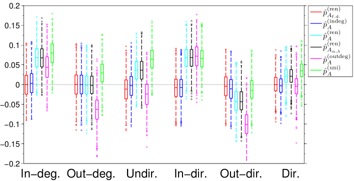
Figure 2: Deviations of estimated $\hat{p}_{A}$ from true value in the directed Erdős-Rényi graphs with $N=1000$, $\alpha=0.75$, $\lambda=10$, $p=0.5$, and $s=500$. Each group of boxplots corresponds to $\hat{p}_{A_{\rm{f.d.}}}^{\rm{(ren)}}$, $\hat{p}_{A}^{\rm{(indeg)}}$, $\hat{p}_{A}^{\rm{(ren)}}$, $\hat{p}_{A_{\alpha,\lambda}}^{\rm{(ren)}}$, $\hat{p}_{A}^{\rm{(outdeg)}}$, and $\hat{p}_{A}^{\rm{(uni)}}$ for one allocation of the individual property $A$. The abbreviations for the allocations corresponds to the function $g$, i.e., In-deg. equals $(d_{i}^{\rm{(un)}}+d_{i}^{\rm{(in)}})$, Out-deg. $(d_{i}^{\rm{(un)}}+d_{i}^{\rm{(out)}})$, Undir. $d_{i}^{\rm{(un)}}$, In-dir. $d_{i}^{\rm{(in)}}$, Out-dir. $d_{i}^{\rm{(out)}}$, and Dir. $(d_{i}^{\rm{(in)}}+d_{i}^{\rm{(out)}})$.

We see that the bias of $\hat{p}_{A_{\rm{f.d}}}^{\rm{(ren)}}$ and $\hat{p}_{A}^{\rm{(indeg)}}$ is small for all allocations, as to be expected. For the estimators utilizing the out-degree, $\hat{p}_{A}^{\rm{(ren)}}$, $\hat{p}_{A_{\alpha,\lambda}}^{\rm{(ren)}}$, and $\hat{p}_{A}^{\rm{(outdeg)}}$, Figure 2 indicates that the choice of how to allocate $A$ has a significant impact on the performance of estimators. When $A$ is allocated proportional to the out-degree (Out-deg. in Fig. 2), $\hat{p}_{A}^{\rm{(ren)}}$ and $\hat{p}_{A_{\alpha,\lambda}}^{\rm{(ren)}}$ yields the most accurate result, and when $A$ is allocated proportional to the number of directed edges (Dir. in Fig. 2), $\hat{p}_{A}^{\rm{(outdeg)}}$ is most accurate; this is true for almost all parameter combinations. In general, the bias and variance increase with both $\alpha$ and $p$ for all estimators, and a small $s$ results in an increased variance, as to be expected. In the Supplementary material, these findings are further illustrated by numerical results with $(\alpha,p,s)$ equal to $(0.5,0.2,500)$, $(0.25,0.5,500)$, and $(0.75,0.5,200)$.

6.2 Networks With Power-law Degree Distributions

To generate power-law networks, we set the expected total number of edges for each node to 16, while we set the expected number of undirected and directed edges equal to $(E(D^{\rm{(un)}}),E(D^{\rm{(in)}}+D^{\rm{(out)}}))=(12,4),(8,8)$, and $(4,12)$. The three cases yield $\alpha=0.25$, 0.5, and 0.75, respectively. For each combination of the parameters, we generate 1000 networks of size $N=1000$ and calculate the mean of the $D_{TV}$. We also calculate the s.d., which is of magnitude $10^{-3}$ and therefore not shown. The sample size $s$ is set to 200 and 500.

The average $D_{TV}$ values for $\hat{\pi}^{\rm{(ren)}}_{\rm{f.d.}}$, $\hat{\pi}^{\rm{(indeg)}}$, $\hat{\pi}^{\rm{(ren)}}$, $\hat{\pi}^{\rm{(ren)}}_{\alpha,\lambda}$, $\hat{\pi}^{\rm{(outdeg)}}$, and $\hat{\pi}^{\rm{(uni)}}$ are shown in Figure 3 for various $\alpha$ and $\gamma$ values. Figure 3 suggests that $\hat{\pi}^{\rm{(ren)}}_{\rm{f.d}}$ and $\hat{\pi}^{\rm{(indeg)}}$ are the most accurate among the four estimators, with $\hat{\pi}^{\rm{(ren)}}_{\rm{f.d}}$ being slightly better. When $\alpha=0.25$ and 0.5, $\hat{\pi}^{\rm{(ren)}}_{\alpha,\lambda}$ has a lower mean $D_{TV}$ than $\hat{\pi}^{\rm{(ren)}}$, but this difference is not seen when $\alpha=0.75$. $\hat{\pi}^{\rm{(outdeg)}}$ performs better than $\hat{\pi}^{\rm{(ren)}}$ for all values of $\gamma$ when $\alpha=0.25$, and the opposite result holds true when $\alpha=0.75$.

Figure 3: Average $D_{TV}$ between the true stationary distribution and $\hat{\pi}^{\rm{(ren)}}_{\rm{f.d.}}$, $\hat{\pi}^{\rm{(indeg)}}$, $\hat{\pi}^{\rm{(ren)}}$, $\hat{\pi}^{\rm{(ren)}}_{\alpha,\lambda}$, $\hat{\pi}^{\rm{(outdeg)}}$, and $\hat{\pi}^{\rm{(uni)}}$ in the power-law networks with $N=1000$, $\alpha$ equal to a) 0.25, b) 0.5, and c) 0.75, and $s=500$.

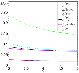
(a) $\alpha=0.25$

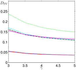
(b) $\alpha=0.5$

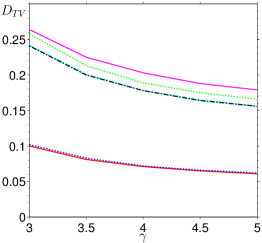
(c) $\alpha=0.75$

In Figure 4, the results for $\hat{p}_{A_{\rm{f.d.}}}^{\rm{(ren)}}$, $\hat{p}_{A}^{\rm{(indeg)}}$, $\hat{p}_{A}^{\rm{(ren)}}$, $\hat{p}_{A_{\alpha,\lambda}}^{\rm{(ren)}}$, $\hat{p}_{A}^{\rm{(outdeg)}}$, and $\hat{p}_{A}^{\rm{(uni)}}$ when $\gamma=3$, $E(D^{\rm{(un)}})=4$, $E(D^{\rm{(in)}}+D^{\rm{(out)}})=12$, $p=0.2$, and $s=500$ are shown. The figure indicates that $\hat{p}_{A_{\rm{f.d.}}}^{\rm{(ren)}}$ and $\hat{p}_{A}^{\rm{(indeg)}}$ have small bias across different allocations of $A$. In contrast, the magnitude of the bias of $\hat{p}_{A}^{\rm{(ren)}}$, $\hat{p}_{A_{\alpha,\lambda}}^{\rm{(ren)}}$, and $\hat{p}_{A}^{\rm{(outdeg)}}$ depends on the allocation type; $\hat{p}_{A}^{\rm{(ren)}}$ has the smallest bias when $A$ is allocated proportional to the undirected degree, and $\hat{p}_{A_{\alpha,\lambda}}^{\rm{(ren)}}$ and $\hat{p}_{A}^{\rm{(outdeg)}}$ when $A$ is allocated proportional to the out-degree. Their relative performance is hard to assess for other allocations. In general, a large fraction of directed edges, small $\gamma$, and large $p$ increase bias and variance, and variance of course decreases with $s$. The Supplementary material contains numerical results for $(\gamma,E(D^{\rm{(un)}}),E(D^{\rm{(in)}}+D^{\rm{(out)}}),p,s)=(4.5,4,12,0.2,500)$, $(4.5,4,12,0.5,500)$, $(4.5,12,4,0.5,500)$, and $(3,4,12,0.2,200)$ to further support these results.

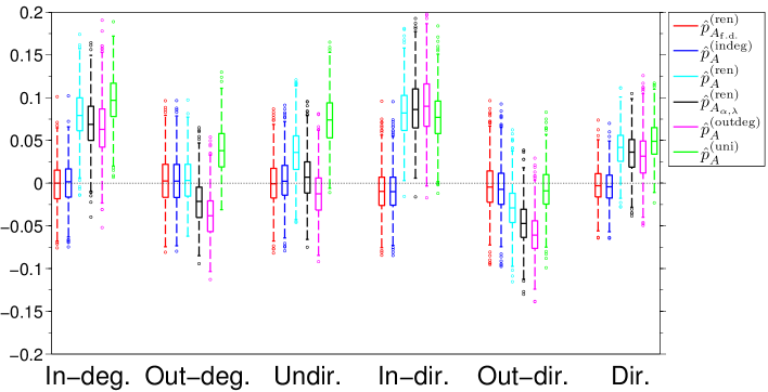
Figure 4: Deviations of estimated $p_{A}$ from the true population proportion in the power-law networks for $\gamma=3$, $E(D^{\rm{(un)}})=4$, $E(D^{\rm{(in)}}+D^{\rm{(out)}})=12$, $p=0.2$, and $s=500$. Each group of boxplots corresponds to $\hat{p}_{A_{\rm{f.d.}}}^{\rm{(ren)}}$, $\hat{p}_{A}^{\rm{(indeg)}}$, $\hat{p}_{A}^{\rm{(ren)}}$, $\hat{p}_{A_{\alpha,\lambda}}^{\rm{(ren)}}$, $\hat{p}_{A}^{\rm{(outdeg)}}$, and $\hat{p}_{A}^{\rm{(uni)}}$, for one allocation of $A$.

6.3 Online MSM Network

For the Qruiser online MSM network, we first evaluate $\hat{\pi}^{\rm{(uni)}}$, $\hat{\pi}^{\rm{(outdeg)}}$, $\hat{\pi}^{\rm{(indeg)}}$, $\hat{\pi}^{\rm{(ren)}}_{\rm{f.d.}}$, and $\hat{\pi}^{\rm{(ren)}}$. The results are shown in Table 4. Note that $\hat{\pi}^{\rm{(ren)}}_{\alpha,\lambda}$ is not evaluated because $\alpha$ and $\lambda$ are not known beforehand. For $\hat{\pi}^{\rm{(uni)}}$, $\hat{\pi}^{\rm{(outdeg)}}$, and $\hat{\pi}^{\rm{(indeg)}}$, $D_{TV}$ to the true selection probabilities is exactly calculated. For $\hat{\pi}^{\rm{(ren)}}_{\rm{f.d.}}$ and $\hat{\pi}^{\rm{(ren)}}$, we show the mean and s.d. of $D_{TV}$ on the basis of 1000 samples of size $500$. We see that $\hat{\pi}^{\rm{(ren)}}_{\rm{f.d.}}$ has smaller $D_{TV}$ than $\hat{\pi}^{\rm{(indeg)}}$, and that the mean $D_{TV}$ of $\hat{\pi}^{\rm{(ren)}}$ is smaller than that of $\hat{\pi}^{\rm{(uni)}}$ and $\hat{\pi}^{\rm{(outdeg)}}$.

Table 4: $D_{TV}$ between the true stationary distribution and $\hat{\pi}^{\rm{(uni)}}$, $\hat{\pi}^{\rm{(outdeg)}}$, $\hat{\pi}^{\rm{(indeg)}}$, $\hat{\pi}^{\rm{(ren)}}_{\rm{f.d.}}$ and $\hat{\pi}^{\rm{(ren)}}$. S.d. is shown in the second row, but only applies to $\hat{\pi}^{\rm{(ren)}}_{\rm{f.d.}}$ and $\hat{\pi}^{\rm{(ren)}}$.

$\hat{\pi}^{\rm{(ren)}}_{\rm{f.d.}}$	$\hat{\pi}^{\rm{(indeg)}}$	$\hat{\pi}^{\rm{(ren)}}$	$\hat{\pi}^{\rm{(outdeg)}}$	$\hat{\pi}^{\rm{(uni)}}$
0.2198	0.2248	0.4057	0.4290	0.4484
0.0004	-	0.0048	-

In Figure 5, we show estimates of the population proportions of the age, county, civil status, and profession properties. The true population proportions are shown by the dashed lines. The sample size is 500. Figure 5 indicates that $\hat{p}_{A_{\rm{f.d.}}}^{\rm{(ren)}}$ performs best of all estimators. Among the estimators utilizing $d_{i}^{\rm{(un)}}+d_{i}^{\rm{(out)}}$, $\hat{p}_{A}^{\rm{(ren)}}$ has the smallest overall bias. Moreover, the variance of $\hat{p}_{A}^{\rm{(ren)}}$ is smaller than for $\hat{p}_{A}^{\rm{(outdeg)}}$ for all properties, in particular the civil status.

Figure 5: Estimates of population proportions in the Qruiser network for a) age, b) civil status, c) county, and d) profession. Each figure shows $\hat{p}_{A_{\rm{f.d.}}}^{\rm{(ren)}}$, $\hat{p}_{A}^{\rm{(indeg)}}$, $\hat{p}_{A}^{\rm{(ren)}}$, $\hat{p}_{A}^{\rm{(outdeg)}}$, and $\hat{p}_{A}^{\rm{(uni)}}$. The true population proportions are shown by the dashed lines and are equal to 0.77, 0.40, 0.39, and 0.38 for age, civil status, county, and profession, respectively.

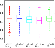
(a)

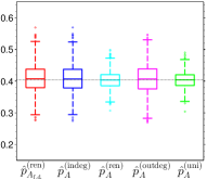
(b)

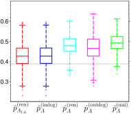
(c)

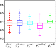
(d)

7 DISCUSSION AND CONCLUSIONS

We developed statistical procedures for sampling vertices in social networks to account for the empirical fact that social networks generally include non-reciprocal edges. The proposed estimation procedures typically outperformed existing methods that neglect directed edges. Among the scenarios investigated in the present study, the best accuracy of estimation was obtained when undirected, in-directed, and out-directed degree are separately observed for sampled individuals. In the more realistic scenario in which one only knows the sum of undirected and out-directed edges of sampled individuals, all estimation procedures are less precise. Our simulations also showed that estimators of population proportions were highly sensitive to how the property $A$ is allocated in the social network.

If the full directed degree $(d_{i}^{\rm{(un)}},d_{i}^{\rm{(in)}},d_{i}^{\rm{(out)}})$ is observed and the moments of the degree distributions are known, our estimator $\hat{\pi}^{\rm{(ren)}}_{\rm{f.d.}}$ is compared to $\hat{\pi}^{\rm{(indeg)}}$. It can be seen in Tables 2 and 4, and Figure 3 that $\hat{\pi}^{\rm{(ren)}}_{\rm{f.d.}}$ performs slightly better than $\hat{\pi}^{\rm{(indeg)}}$ in all the studied situations. The corresponding estimated proportions given by $\hat{p}_{A_{\rm{f.d.}}}^{\rm{(ren)}}$ and $\hat{p}_{A}^{\rm{(outdeg)}}$ in Figures 2, 4, and 5 are very similar.

If only the out-degree $d_{i}^{\rm{(un)}}+d_{i}^{\rm{(out)}}$ is observed, we compare $\hat{\pi}^{\rm{(ren)}}$ and $\hat{\pi}^{\rm{(outdeg)}}$ (Tables 3 and 4, and Figure 3). We also include $\hat{\pi}^{\rm{(ren)}}_{\alpha,\lambda}$ in the comparison on the generated networks, and it can be seen that the performance of $\hat{\pi}^{\rm{(ren)}}_{\alpha,\lambda}$ is only slightly better than that of $\hat{\pi}^{\rm{(ren)}}$. Our estimator $\hat{\pi}^{\rm{(ren)}}$ outperforms $\hat{\pi}^{\rm{(outdeg)}}$ except when the fraction of directed edges $\alpha$ is small (0.1 in Table 3 and 0.25 in Figure 3). This corresponds to that $\hat{\pi}^{\rm{(ren)}}$ will deviate further from $\hat{\pi}^{\rm{(outdeg)}}$ as $\alpha$ increases (Eq. (14)). Figures 2 and 4 indicate that the results of the estimators $\hat{p}_{A}^{\rm{(ren)}}$, $\hat{p}_{A_{\alpha,\lambda}}^{\rm{(ren)}}$, and $\hat{p}_{A}^{\rm{(outdeg)}}$ depend much on the allocation of the property $A$. We believe that it is of interest to further study how properties are distributed in empirical social networks.

If $\alpha$ is known, we can estimate $\lambda$ using only the mean sample out-degree in Eq. (13). Although generally difficult, it is possible to assess the fraction of directed edges in the social network of a hidden population through direct methods. In many RDS studies, participants are asked questions that experimenters use to quantify the nature of the relationship between a participant and its recruiter, e.g., friends, acquantiances or strangers (e.g., Ramirez-Valles et al.,, 2005; Wang et al.,, 2007; Ma et al.,, 2007). With these questions, the authors aim to control for non-reciprocated relationships, which could lead to the participant being excluded from the sample. This type of questions is also useful for assessing the directedness of the social network, because the fraction of coupons given by strangers could be a measure of (non-)reciprocity. In Gile et al., (2012), another type of question more directly assessing reciprocation is suggested, e.g. “Do you think that the person to whom you gave a coupon would have given you a coupon if you had not participated in the study first?”. Another possible method to estimate $\alpha$ would be to obtain information on the number of revisits $m$ used in Eq. (12). This could be done by asking for example “Would you give a coupon to the person who gave you a coupon if he or she had not yet participated in the study?”.

The main focus of the present paper was on accounting for directed edges in a social network. There are also other assumptions in existing estimation procedures (including the current one) worthy of relaxing. For example, the methods typically assume that participants choose coupon recipents uniformly at random among their neighbors in the social network. In reality, they probably sample closely connected neighbors more likely, which may bias estimators of selection probabilities. Extending the RDS methods by allowing weighted edges warrants for future work. It should be noted that our methods allow the two weights on the same undirected edge in the opposite directions to be different, because our framework targets directed networks.

Random walks on directed networks have numerous other applications, including identification of important vertices (Brin and Page,, 1998; Langville and Meyer,, 2006; Noh and Rieger,, 2004; Newman,, 2005) and community detection (Rosvall and Bergstrom,, 2008). Therefore, we also hope that this work may contribute to an increased understanding in other areas of network research that use random walks on directed networks.

References

- Boldi et al., (2011) Boldi, P., Rosa, M., Santini, M., and Vigna, S. (2011). Layered label propagation: A multiresolution coordinate-free ordering for compressing social networks. In Proceedings of the 20th international conference on World Wide Web, pages 587–596. ACM.