QuPARA: Query-Driven Large-Scale Portfolio
Aggregate Risk Analysis on MapReduce

Abstract

Modern insurance and reinsurance companies use stochastic simulation techniques for portfolio risk analysis. Their risk portfolios may consist of thousands of reinsurance contracts covering millions of individually insured locations. To quantify risk and to help ensure capital adequacy, each portfolio must be evaluated in up to a million simulation trials, each capturing a different possible sequence of catastrophic events (e.g., earthquakes, hurricanes, etc.) over the course of a contractual year.

In this paper, we explore the design of a flexible framework for portfolio risk analysis that facilitates answering a rich variety of catastrophic risk queries. Rather than aggregating simulation data in order to produce a small set of high-level risk metrics efficiently (as is often done in production risk management systems), the focus here is on allowing the user to pose queries on unaggregated or partially aggregated data. The goal is to provide a flexible framework that can be used by analysts to answer a wide variety of unanticipated but natural ad hoc queries. Such detailed queries can help actuaries or underwriters to better understand the multiple dimensions (e.g., spatial correlation, seasonality, peril features, construction features, financial terms, etc.) that can impact portfolio risk and thus company solvency.

We implemented a prototype system, called QuPARA (Query-Driven Large-Scale Portfolio Aggregate Risk Analysis), using Hadoop, which is Apache’s implementation of the MapReduce paradigm. This allows the user to take advantage of large parallel compute servers in order to answer ad hoc risk analysis queries efficiently even on very large data sets typically encountered in practice. We describe the design and implementation of QuPARA and present experimental results that demonstrate its feasibility. A full portfolio risk analysis run consisting of a 1,000,000 trial simulation, with 1,000 events per trial, and 3,200 risk transfer contracts can be completed on a 16-node Hadoop cluster in just over 20 minutes.

I Introduction

At the heart of the analytical pipeline of a modern insurance/reinsurance company is a stochastic simulation technique for portfolio risk analysis and pricing referred to as Aggregate Analysis [1, 2, 3, 4]. At an industrial scale, a risk portfolio may consist of thousands of annual reinsurance contracts covering millions of individually insured locations. To quantify annual portfolio risk, each portfolio must be evaluated in up to a million simulation trials, each consisting of a sequence of possibiliy thousands of catastrophic events, such as earthquakes, hurricanes or floods. Each trial captures one scenario how globally distributed catastrophic events may unfold in a year.

Aggregate analysis is computationally intensive as well as data-intensive. Production analytical pipelines exploit parallelism in aggregate risk analysis and ruthlessly aggregate results. The results obtained from production pipelines summarize risk in terms of a small set of standard portfolio metrics that are key to regulatory bodies, rating agencies, and an organisation’s risk management team, such as Probable Maximum Loss (PML) [5, 6] and Tail Value-at-Risk (TVaR) [7, 8]. While production pipelines can efficiently aggregate terabytes of simulation results into a small set of key portfolio risk metrics, they are typically very poor at answering the types of ad hoc queries that can help actuaries or underwriters to better understand the multiple dimensions of risk that can impact a portfolio, such as spatial correlation, seasonality, peril features, construction features, and financial terms.

This paper proposes a framework for aggregate risk analysis that facilitates answering a rich variety of ad hoc queries in a timely manner. A key characteristic of the proposed framework is that it is designed to allow users with extensive mathematical and statistical skills but perhaps limited programming background, such as risk analysts, to pose a rich variety of complex risk queries. The user formulates their query by defining SQL-like filters. The framework then answers the query based on these filters, without requiring the user to make changes to the core implementation of the framework or to reorganize the input data of the analysis. The challenges that arise due to the amounts of data to be processed and due to the complexity of the required computations are largely encapsulated within the framework and hidden from the user.

Our prototype implementation of this framework for Query-Driven Large-Scale Portfolio Aggregate Risk Analysis, referred to as QuPARA, uses Apache’s Hadoop [9, 10] implementation of the MapReduce programming model [11, 12, 13] to exploit parallelism, and Apache Hive [14, 15] to support ad hoc queries. Even though QuPARA is not as fast as a production system on the narrow set of standard portfolio metrics, it can answer a wide variety of ad hoc queries in an efficient manner. For example, our experiments demonstrate that an industry-size risk analysis with 1,000,000 simulation trials, 1,000 events per trial, and on a portfolio consisting of 3,200 risk transfer contracts (layers) with an average of 5 event loss tables per layer can be carried out on a 16-node Hadoop cluster in just over 20 minutes.

The remainder of this paper is organized as follows. Section II gives an overview of reinsurance risk analysis. Section III proposes our new risk analysis framework. Section IV considers an example query processed by the framework and various queries for fine-grained aggregate risk analysis. Section V describes implementation details. Section VI presents a performance evaluation of our framework. Section VII presents conclusions and discusses future work.

II An Overview of Risk Analysis

A reinsurance company typically holds a portfolio of programs that insure primary insurance companies against large-scale losses, like those associated with catastrophic events. Each program contains data that describes (1) the buildings to be insured (the exposure), (2) the modelled risk to that exposure (the event loss tables), and (3) a set of risk transfer contracts (the layers).

The exposure is represented by a table, one row per building covered, that lists the building’s location, construction details, primary insurance coverage, and replacement value. The modelled risk is represented by an event loss table (ELT). This table lists for each of a large set of possible catastrophic events the expected loss that would occur to the exposure should the event occur. Finally, each layer (risk transfer contract) is described by a set of financial terms that includes aggregate deductibles and limits (i.e., deductibles and maximal payouts to be applied to the sum of losses over the year) and per-occurrence deductibles and limits (i.e., deductibles and maximal payouts to be applied to each loss in a year), plus other financial terms.

Consider, for example, a Japanese earthquake program. The exposure might list 2 million buildings (e.g., single-family homes, small commercial buildings, and apartments) and, for each, its location (e.g., latitude and longitude), constructions details (e.g., height, material, roof shape, etc.), primary insurance terms (e.g., deductibles and limits), and replacement value. The event loss table might, for each of 100,000 possible earthquake events in Japan, give the sum of the losses expected to the associated exposure should the associated event occur. Note that ELTs are the output of stochastic region peril models [17] and typically also include some additional financial terms. Finally, a risk transfer contract may consist of two layers as shown in Figure 1. The first layer is a per-occurrence layer that pays out a 60% share of losses between 160 million and 210 million associated with a single catastrophic event. The second layer is an aggregate layer covering 30% of losses between 40 million and 90 million that accumulate due to earthquake activity over the course of a year.

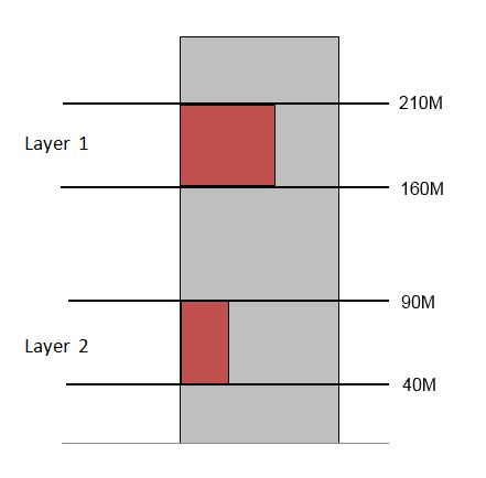
Figure 1: An example two-layer reinsurance program.

Given a reinsurance company’s portfolio described in terms of exposure, event loss tables, and layers, the most fundamental type of analysis query computes an Exceedance Probability (EP) curve, which represents, for each of a set of user-specified loss values, the probability that the total claims a reinsurer will have to pay out exceeds this value. Not surprisingly there is no computationally feasible closed-form expression for computing such an EP curve over hundreds of thousands of events and millions of individual exposures. Consequently a simulation approach must be taken. The idea is to perform a stochastic simulation based on a year event table (YET). This table describes a large number of trials, each representing one possible sequence of catastrophic events that might occur in a given year. This YET is generated by an event simulator that uses the expected occurrence rate of each event plus other hazard information like seasonality. The process to generate the YET is beyond the scope of this paper, and we focus on the computationally intensive task of computing the expected loss distribution (i.e., EP curve) for a given portfolio, given a particular YET. Given the sequence of events in a given trial, the loss for this particular trial can be computed, and the overall loss distribution is obtained from the losses computed for the set of trials.

While computing the EP curve for the company’s entire portfolio is critical in assessing a company’s solvency, analysts are often interested in digging deeper into the data and posing a wide variety of queries with the goal of analysing such things as cash flow throughout the year, diversity of the portfolio, financial impact of adding a new contract or contracts to the portfolio, and many others.

The following is a representative, but far from complete, set of example queries. Note that while all of them involve some aspects of the basic aggregate risk analysis algorithm used to compute Exceedance Probability curves, each puts its own twist on the computation.

EP Curves with secondary uncertainty:

In the basic aggregate risk analysis algorithm, the loss value for each event is represented by a mean value. This is an oversimplification because for any given event there are a multitude of possible loss outcomes. This means that each event has an associated probability distribution of loss values rather than a single associate loss value. Secondary uncertainty arises from the fact that we are not just unsure whether an event will occur (primary uncertainty) but also about many of the exposure and hazard parameters and their interactions.

Performing aggregate risk analysis accounting for secondary uncertainty (i.e., working with the loss distributions associated with events rather than just mean values) is computationally intensive due to the statistical tools employed—for example, the beta probability distribution is employed in estimating the loss using the inverse beta cumulative density function [16]—but is essential in many applications.

Return period losses (RPL)

by line of business (LOB), class of business (COB) or type of participation (TOP): In the reinsurance industry, a layer defines coverage on different types of exposures and the type of participation. Exposures can be classified by class of business (COB) or line of business (LOB) (e.g., marine, property or engineering coverage). The way in which the contractual coverage participates when a catastrophic event occurs is defined by the type of participation (TOP). Decision makers may want to know the loss distribution of a specific layer type in their portfolios, which requires the analysis to be restricted to layers covering a particular LOB, COB or TOP.

Region/peril losses:

This type of query calculates the expected losses or a loss distribution for a set of geographic regions (e.g., Florida or Japan), a set of perils (e.g., hurricane or earthquake) or a combination of region and peril. This allows the reinsurer to understand both what types of catastrophes provide the most risk to their portfolio and in which regions of the globe they are most heavily exposed to these risks. This type of analysis helps the reinsurer to diversify or maintain a persistent portfolio in either dimension or both.

Multi-marginal analysis:

Given the current portfolio and a small set of potential new contracts, a reinsurer will have to decide which contracts to add to the portfolio. Adding a new contract means additional cash flow but also increases the exposure to risk. To help with the decision which contracts to add, multi-marginal analysis calculates the difference between the loss distributions for the current portfolio and for the portfolio with any subset of these new contracts added. This allows the insurer to choose contracts or to price the contracts so as to obtain the “right” combination of added cash flow and added risk.

Stochastic exceedance probability (STEP) analysis:

This analysis is a stochastic approach to the weighted convolution of multiple loss distributions. After the occurrence of a natural disaster not in their event catalogue, catastrophe modelling [17] vendors attempt to estimate the distribution of possible loss outcomes for that event. One way of doing this is to find similar events in existing stochastic event catalogues and propose a weighted combination of the distributions of several events that best represents the actual occurrence. A simulation-based approach allows for the simplest method of producing this combined distribution. To perform this type of analysis, a customized Year Event Table must be produced from the selected events and their weights. In this YET, each trial contains only one event, chosen with a probability proportional to its weight. The final result is a loss distribution of the event, including various statistics such as mean, variance and quantiles.

Periodic Loss Distribution:

Many natural catastrophes have a seasonal component to them, that is, do not occur uniformly throughout the year. For example, hurricanes on the Atlantic coast occur between July and November. Flooding in equatorial regions occurs in the rain season. As a result, the reinsurer may be interested in how their potential losses fluctuate throughout the year, for example to reduce their exposure through reduced contracts or increased retrocessional coverage during riskier periods. To aid in these decisions, a periodic loss distribution represents the loss distribution for different periods of the year, such as quarters, months, weeks, etc.

III QuPARA Framework

In this section, we present our QuRARA framework. Before describing QuPARA, we give an overview of the steps involved in answering an aggregate query sequentially. This will be helpful in understanding the parallel evaluation of aggregate queries using QuPARA.

The loss distribution is computed from the portfolio and the YET in two phases. The first phase computes a year loss table (YLT). For each trial in the YET, each event in this trial, and each ELT that includes this event, the YLT contains a tuple $\langle$trial, event, ELT, loss$\rangle$ recording the loss incurred by this event, given the layer’s financial terms and the sequence of events in the trial up to the current event. The second phase then aggregates the entries in the YLT to compute the final loss distribution. Algorithm 1 shows the sequential computation of the YLT.

Input: Portfolio and YET

Output: YLT

1 for each trial $T$ in the YET do

2      for each event $X$ in $T$ do

3            for each program $P$ in the portfolio do

4                  for each layer $L$ in $P$ do

5                        for each ELT $E$ covered by $L$ do

6                               Lookup $X$ in $E$ to determine the loss $l_{X}$ associated with $X$

7                               $l_{L}\leftarrow$ $l_{L}$ + $l_{X}$

8                              

9                         Apply per-occurrence and aggregate financial terms to $l_{L}$

10                         $l_{P}\leftarrow$ $l_{P}$ + $l_{L}$

11                        

12                   $l_{PF}\leftarrow$ $l_{PF}$ + $l_{P}$

13                  

14             $l_{T}\leftarrow$ $l_{T}$ + $l_{PF}$

15            

16       Populate $YLT$

Algorithm 1 Sequential Aggregate Risk Analysis

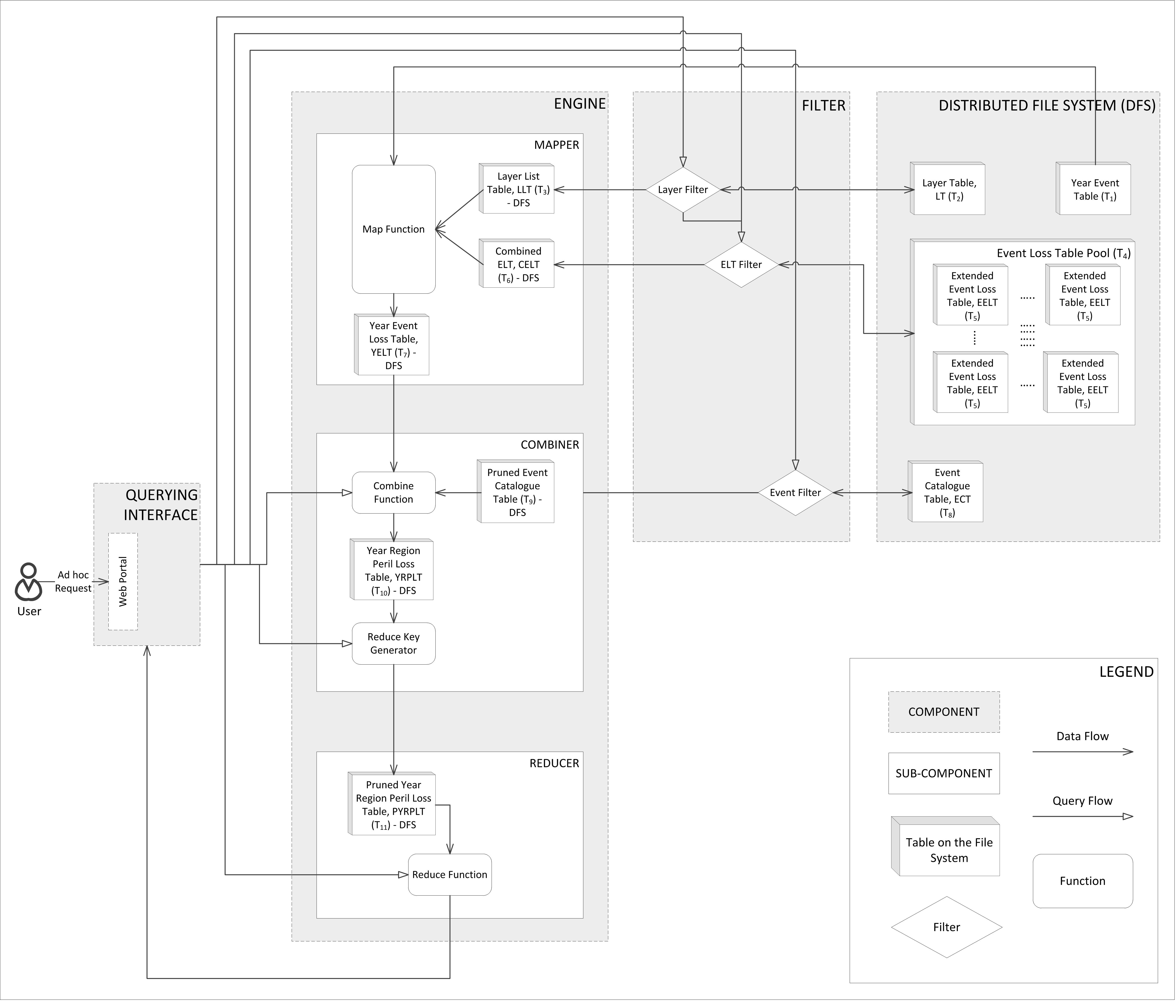
Figure 2: The Query-Driven Portfolio Aggregate Risk Analysis (QuPARA) Framework

After looking up the losses incurred by a given event in the ELTs of a given layer and summing these losses, the resulting layer loss $l_{L}$ is reduced by applying the layer’s per-occurrence and aggregate financial terms. The remaining loss is added to the program loss $l_{P}$ for this event, which in turn is added tho the portfolio loss $l_{PF}$ for this event. Finally, the loss of an entire trial, $l_{T}$ is computed by summing the portfolio losses for all events in the trial. Depending on the level of detail of the final analysis, the YLT is populated with the loss values at different levels of aggregation. At one extreme, if only the loss distribution for the entire portfolio is of interest, there is one loss value per trial. At the other extreme, if the filtering of losses based on some combination of region, peril, LOB, etc. is required, the YLT contains one loss value for each $\langle$trial, program, layer, ELT, event$\rangle$ tuple.

In order to answer ad hoc aggregate queries efficiently, our QuPARA framework provides a parallel implementation of such queries using the MapReduce programming model. The computation of the YLT is the responsibility of the mapper, while the computation of the final loss distribution(s) is done by the reducer. Next we describe the components of QuPARA.

III-A Components

Figure 2 visualizes the design of QuPARA. The framework is split into a front-end offering a query interface to the user, and a back-end consisting of a distributed file system and a query engine that executes the query using MapReduce. As already stated, the user poses a query to the query interface using an SQL-like syntax and does not need to have any knowledge of the implementation of the back-end.

The query interface offers a web-based portal through which the user can issue ad hoc queries in an SQL-like syntax. The query is then parsed and passed to the query engine.

The distributed file system, implemented using Hadoop’s HDFS, stores the raw portfolio data, as well as the YET in tabular form.

The query engine employs the MapReduce framework to evaluate the query using a single round consisting of a map/combine step and a reduce step. During the map step, the engine uses one mapper per trial in the YET, in order to construct a YLT from the YET, equivalent to the sequential construction of the YLT from the YET using Algorithm 1. The combiner and reducer collaborate to aggregate the loss information in the YLT into the final loss distribution for the query. There is one combiner per mapper. The combiner pre-aggregates the loss information produced by this mapper, in order to reduce the amount of data to be sent across the network to the reducer(s) during the shuffle step. The reducer(s) then carry out the final aggregation. In most queries, which require only a single loss distribution as output, there is a single reducer. Multi-marginal analysis is an example where multiple loss distributions are to be computed, one per subset of the potential contracts to be added to the portfolio. In this case, we have one reducer for each such subset, and each reducer produces the loss distribution for its corresponding subset of contracts.

Each mapper retrieves the set of ELTs required for the query from the distributed file system using a layer filter and an ELT filter. Specifically, the query may specify a subset of the layers in the portfolio to be the subject of the analysis. The layer filter retrieves the identifiers of the ELTs contained in these layers from the layer table. If the query specifies, for example, that the analysis should be restricted to a particular type of peril, the ELT filter then extracts from this set of ELTs the subset of ELTs corresponding to the specified type of peril. Given this set of ELT identifiers, the mapper retrieves the actual ELTs and, in memory, constructs a combined ELT associating a loss with each $\langle$event, ELT$\rangle$ pair. It then iterates over the sequence of events in its trial, looks up the ELTs recording non-zero losses for each event, and generates the corresponding $\langle$trial, event, ELT, loss$\rangle$ tuple in the YLT, taking each ELT’s financial terms into account.

The aggregation to be done by the combiner depends on the query. In the simplest case, a single loss distribution for the selected set of layers and ELTs is to be computed. In this case, the combiner sums the loss values in the YLT output by the mapper and sends this aggregate value to the reducer. A more complicated example is the computation of a weekly loss distribution. In this case, the combiner would aggregate the losses corresponding to the events in each week and send each aggregate to a different reducer. Each reducer is then responsible for computing the loss distribution for one particular week.

A reducer, finally, receives one loss value per trial. It sorts these loss values in increasing order and uses this sorted list to generate a loss distribution.

The following is a more detailed description of the mapper, combiner, and reducer used to implement parallel aggregate risk analysis in MapReduce.

III-A1 Mapper

The mapper, shown in Algorithm 2, takes as input an entire trial and the list of its events, represented as a pair $\langle$$T,E:=\{E_{1},E_{2},\dots,E_{m}\}$$\rangle$. Algorithm 2 does not show the construction of the combined ELT (CELT) and layer list (LLT) performed by the mapper before carrying out the steps in lines 1–9. The loss estimate of an event in a portfolio is computed by scanning through every layer $L$ in the LLT, retrieving and summing the loss estimates for all ELTs covered by this layer, and finally applying the layer’s financial terms.

Input: $\langle$$T,E:=\{E_{1},E_{2},\cdots,E_{m}\}$$\rangle$, where $m$ is the number of events in a trial

Output: A list of entries $\langle$$T,E_{i},l_{PF}$$\rangle$ of the YLT

1 for each event, $E_{i}$ in $E$ do

2       Look up $E_{i}$ in the CELT and find corresponding losses, $l_{E_{i}}=\{l^{1}_{E_{i}},l^{2}_{E_{i}},\cdots,l^{n}_{E_{i}}\}$, where ELT₁, ELT₂, …, ELT_n are the ELTS in the CELT

3       for each layer, $L$, in the LLT do

4             for each ELT ELT_j covered by $L$ do

5                   Lookup $l^{j}_{E_{i}}$ in $l_{E_{i}}$

6                   $l_{L}\leftarrow$ $l_{L}$ + $l^{j}_{E_{i}}$

7                  

8             Apply $L$’s financial terms to $l_{L}$

9             $l_{PF}\leftarrow l_{PF}+l_{L}$

10       Emit($\langle$$T$, $E_{i}$, $l_{PF}$$\rangle$)

Algorithm 2 Mapper in parallel aggregate risk analysis

III-A2 Combiner

The combiner, shown in Algorithm 3, receives as input the list of triples $\langle$$T$, $E_{i}$, $l_{PF}$$\rangle$ generated by a single mapper, that is, the list of loss values for the events in one specific trial. The combiner groups these loss values according to user-specified grouping criteria and outputs one aggregate loss value per group.

Input: A list of YLT entries $\langle$$T$, $E_{i}$, $l_{PF}$$\rangle$ for the events in a given trial $T$.

Output: A list of aggregate YLT entries $\langle$$G_{i}$, $T$, $l_{G}$$\rangle$ with key $G_{i}$ for the event groups in trial $T$

1 Join input tuples with event catalogue to annotate events with their attributes (region, peril, etc.)

2 Group events in the input list by event features according to the user’s query

3 for each group $G_{i}$ do

4       $l_{G_{i}}\leftarrow{}$sum of the loss values associated with the events in $G_{i}$ in trial $T$

5       Emit($\langle$$T$, $G_{i}$, $L_{G}$$\rangle$)

Algorithm 3 Combiner in parallel aggregate risk analysis

III-A3 Reducer

The reducer, shown in Algorithm 4, receives as input the loss values for one specific group and for all trials in the YET. The reducer then aggregates these loss values into the loss statistic requested by the user. For example, to generate an exceedance probability curve, the reducer sorts the received loss values in increasing order and, for each loss value $v$ in a user-specified set of loss values, reports the percentage of trials with a loss value greater than $v$ as the probability of incurring a loss higher than $v$.

Input: A list of loss tuples $\langle$$G_{i}$, $T$, $l_{PF}$$\rangle$ for an event group $G_{i}$.

Output: Loss statistics for event group $G_{i}$ based on user’s query

1 Based on user query, generate: (i) Group loss distribution, or (ii) Group loss statistics, or (iii) Group value-at-risk (VaR) and/or Tail value-at-risk (TVaR), or (iv) Exceedance probability curves

Algorithm 4 Reducer in parallel aggregate risk analysis

III-B Data Organization

The data used by QuPARA is stored in a number of tables:

• The year event table YET contains tuples $\langle$trial_ID, event_ID, time_Index, z_PE$\rangle$. trial_ID is a unique identifier associated with each of the one million trials in the simulation. event_ID is a unique identifier associated with each event in the event catalogue. time_Index determines the position of the occurrence of the event in the sequence of events in the trial. z_PE is a random number specific to the program and event occurrence. Each event occurrence across different programs has a different associated random number.

• The layer table LT contains tuples $\langle$layer_ID, cob, lob, tob, elt_IDs$\rangle$. layer_ID is a unique identifier associated with each layer in the portfolio. cob is an industry classification according to perils insured and the related exposure and groups homogeneous risks. lob defines a set of one or more related products or services where a business generates revenue. tob describes how reinsurance coverage and premium payments are calculated. elt_IDs is a list of event loss table IDs that are covered by the layer.

• The layer list table LLT contains tuples $\langle$layer_ID, occ_Ret, occ_Lim, agg_Ret, agg_Lim$\rangle$. Each entry is a simplified representation of the layer identified by layer_ID. occ_Ret is the occurrence retention or deductible of the insured for an individual occurrence loss. occ_Lim is the occurrence limit or coverage the insurer will pay for occurrence losses in excess of the occurrence retention. agg_Ret is the aggregate retention or deductible of the insured for an annual cumulative loss. agg_Lim is the aggregate limit or coverage the insurer will pay for annual cumulative losses in excess of the aggregate retention.

• The event loss table pool ELTP contains tuples $\langle$elt_ID, region, peril$\rangle$. Each such entry associates a particular type of peril and a particular region with the ELT with ID elt_ID.

• The extended event loss table EELT contains tuples $\langle$event_ID, z_E, mean_Loss, sigma_I, sigma_C, max_Loss$\rangle$. event_ID is the unique identifier of an event in the event catalogue. z_E is a random number specific to the event occurrence. Event occurrences across different programs have the same random number. mean_Loss denotes the mean loss incurred if the event occurs. max_Loss is the maximum expected loss incurred if the event occurs. sigma_I represents the variance of the loss distribution for this event. sigma_C represents the error of the event-occurrence dependencies.

• The combined event loss table CELT is not stored on disk but is constructed by each mapper in memory from the extended event loss tables corresponding to the user’s query. It associates with each event ID event_ID a list of tuples $\langle$elt_ID, z_E, mean_Loss, sigma_I, sigma_C, max_Loss$\rangle$, which is the loss information for event event_ID stored in the extended ELT elt_ID.

• The year event loss table YELT is an intermediate table produced by the mapper for consumption by the combiner. It contains tuples $\langle$trial_ID, event_ID, time_Index, estimated_Loss$\rangle$.

• The event catalogue ECT contains tuples $\langle$event_ID, region, peril$\rangle$ associating a region and a type of peril with each event.

• The year region peril loss table YRPLT contains tuples $\langle$trial_ID, time_Index, region, peril, estimated_Loss$\rangle$, listing for each trial the estimated loss at a given time, in a given region, and due to a particular type of peril. This is yet another intermediate table, which is produced by the combiner for consumption by the reducer.

III-C Data Filters

QuPARA incorporates three types of data filters that allow the user to focus their queries on specific geographic regions, types of peril, etc. These filters select the appropriate entries from the data tables they operate on, for further processing my the mapper, combiner, and reducer.

• The layer filter extracts the set of layers from the layer table LT and passes this list of layers to the mapper as the “portfolio” to be analyzed by the query. The list of selected layers is also passed to the ELT filter for selection of the relevant ELTs.

• The ELT filter is used to select, from the ELT pool ELTP, the set of ELTs required by the layer filter and for building the combined ELT CELT.

• The event filter selects the features of events from the event catalogue ECT to provide the grouping features to the combiner.

IV An Example Query

An example of an ad hoc request on QuPARA is to generate a report on seasonal loss value-at-risk (VaR) with confidence level of 99% due to hurricanes and floods that affects all commercial properties in different locations in Florida. The user poses the query through the query interface, which translates the query into a set of five SQL-like queries to be processed by the query engine:

$Q_{1}$:

The first part of processing any user query is the query to be processed by the layer filter. In this case, we are interested in all layers covering commercial properties, which translates into the following SQL query:

  SELECT * FROM LT
  WHERE lob IN commercial

$Q_{2}$:

The second query is processed by the ELT filter to extract the ELTs relevant for the analysis. In this case, we are interested in all ELTs covered by layers returned by query $Q_{1}$ and which cover Florida (FL) as the region and hurricanes (HU) and floods (FLD) as perils:

  SELECT elt_ID FROM ELTP
  WHERE elt_ID IN Q1
  AND region IN FL
  AND peril IN HU, FLD

$Q_{3}$:

This query is provided to the event filter for retrieving event features required for grouping estimated losses in the YELT.

  SELECT event_ID AND region FROM YELT

$Q_{4}$:

This query is provided to the combiner for grouping all events in a trial based on their order of occurrence. For example, if there are 100 events equally distributed in a year and need to be grouped based on the four seasons in a year, then the estimated loss for each season is the sum of 25 events that occur in that season.

  SELECT trial_ID,
  SEASON_SUM(estimated_Loss)
  FROM YELT
  GROUP BY time_Index

$Q_{5}$:

This query is provided to the reducer to define the final output of the user request. The seasonal loss Value-at-Risk (VaR) with 99% confidence level is estimated.

  SELECT VaR IN 0.01 FROM YRPLT

V Implementation

For our implementation of QuPARA, we used Apache Hadoop, an open-source software framework that implements the MapReduce programming model [9, 10, 18]. We chose Hadoop because other available frameworks [20, 21] require the use of additional interfaces, commercial or web-based, for deploying an application.

A number of interfaces provided by Hadoop, such as the InputFormat and the OutputFormat are implemented as classes. The Hadoop framework works in the following way for a MapReduce round. The data files are stored on the Hadoop Distributed File System (HDFS) [19] and are loaded by the mapper. Hadoop provides an InputFormat interface, which specifies how the input data is to be split for processing by the mapper. HDFS provides an additional functionality, called distributed cache, for distributing small data files that are shared by the nodes of the cluster. The distributed cache provides local access to the shared data. The Mapper interface receives the partitioned data and emits intermediate key-value pairs. The Partitioner interface receives the intermediate key-value pairs and controls the partitioning of these keys for the Reducer interface. Then the Reducer interface receives the partitioned intermediate key-value pairs and generates the final output of this MapReduce round. The output is received by the OutputFormat interface and provides it back to HDFS.

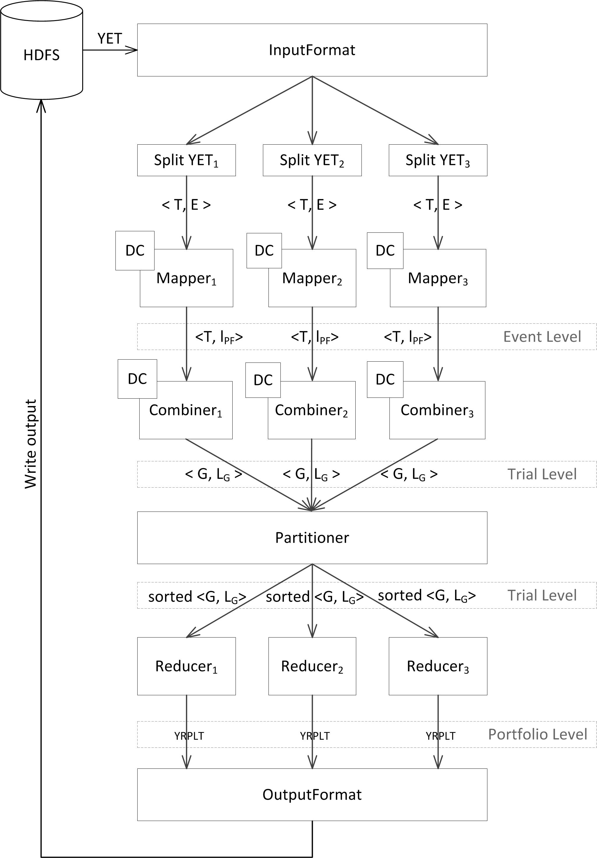
Figure 3: Apache Hadoop for MapReduce in the QuPARA Framework

The input data for a MapReduce round in QuPARA is the year event table YET, the event loss table pool ELTP, the list of layers LT, and the event catalogue ECT, which are stored on HDFS. The master node executes Algorithm 5 and requires access to the ELT pool and the portfolio before the MapReduce round. Firstly, the master node uses the portfolio to decompose the aggregate analysis job into a set of sub-jobs $\{J_{1},\cdots,J_{x}\}$ as shown in line 1, each covering 200 layers. This partition into sub-jobs was chose to ensure a balance between Input/Output cost and the overhead for (sequentially) constructing the combined ELT in each mapper; more sub-jobs means reading the YET more often, whereas fewer and larger jobs increase the overhead of the sequential combined ELT construction. The layers and the corresponding ELTs required by each sub-job are then submitted to the Hadoop job scheduler in lines 2–6. The MapReduce round is illustrated in Figure 3.

Input: ELT pool, portfolio

1 Split the portfolio into jobs $J_{1},\cdots,J_{x}$

2 for each Job $J_{i}$ do

3       Distribute its layers to nodes via the distributed cache

4       for each layer $L_{j}$ in job $J_{i}$ do

5             Distribute the ELTs covered by $L_{j}$ to nodes via the distributed cache

6            

7       Submit $J_{i}$ to Hadoop job scheduler

8      

Algorithm 5 Algorithm for master node in aggregate risk analysis

The InputFormat interface splits the YET based on the number of mappers specified for the MapReduce round. By default, Hadoop splits large files based on HDFS block size, but in this paper, the InputFormat is redefined to split files based on the number of mappers. The mappers are configured so that they receive all the ELTs covered by the entire portfolio via the distributed cache. Each mapper then constructs its own copy of the combined ELT form the ELTs in the distributed cache. Using a combined ELT speeds up the lookup of events in the relevant ELTs in the subsequent processing of the events in the YET. If individual ELTs were employed, then one lookup would be required for fetching the loss value of an event from each ELT. Using a combined ELT, only a single lookup is required. The mapper now implements Algorithm 2 to compute the loss information for all events in its assigned portion of the YET.

The combiner implements Algorithm 3 to group the event-loss pairs received from the mapper and emits the group-loss pairs to the partitioner. The event catalogue is contained in the distributed cache of the combiner and is used by the combiner to implement the grouping of events. The Combiner delivers the grouped loss pairs to the partitioner. The partitioner ensures that all the loss pairs with the same group key are delivered to the same reducer.

The reducer implements Algorithm 4 to collect the sorted group-loss pairs and produces year region peril loss table YRPLT. Based on the query, the OutputFormat generates reports which are then saved to the HDFS.

The layer filter, ELT filter, and event filter, described earlier, are implemented using Apache Hive [14], which is built on top of the Hadoop Distributed File System and supports data summarization and ad hoc queries using an SQL-like language.

VI Performance Evaluation

In this section, we discuss our experimental setup for evaluating the performance of QuPARA and the results we obtained.

VI-A Platform

We evaluated QuPARA on the Glooscap cluster of the Atlantic Computational Excellence Network (ACEnet). We used 16 nodes of of the cluster, each of which was an SGI C2112-4G3 with four quad-core AMD Opteron 8384 (2.7 GHz) processors and 64 GB RAM per node. The nodes were connected via Gigabit Ethernet. The operating system on each node was Red Hat Enterprise Linux 4.8. The global storage capacity of the cluster was 306 TB of Sun SAM-QFS, a hierarchical storage system using RAID 5. Each node had 500GB of local storage. The Java Virtual Machine (JVM) version was 1.6. The Apache Hadoop version was 1.0.4. The Apache Hive version was 0.10.0.

VI-B Results

Figure 4 shows the total time taken in seconds for performing aggregate risk analysis on our experimental platform. Up to 16 nodes were used in the experiment. Each node processed one job with 200 layers, each covering 5 unique ELTs. Thus, up to 16,000 ELTs were considered. The YET in our experiments contained 1,000,000 trials, each consisting of 1,000 events. The graph shows a very slow increase in the total running time, in spite of the constant amount of computation to be performed by each node (because every node processes the same number of layers, ELTs, and YET entries). The gradual increase in the running time is due to the increase in the setup time required by the Hadoop job scheduler and the increase in network traffic (reflected in an increase in the time taken by the reducer). Nevertheless, this scheduling and network traffic overhead amounted to only 1.67%–7.13% of the total computation time. Overall, this experiment demonstrates that, if the hardware scales with the input size, QuPARA’s processing time of a query remains nearly constant.

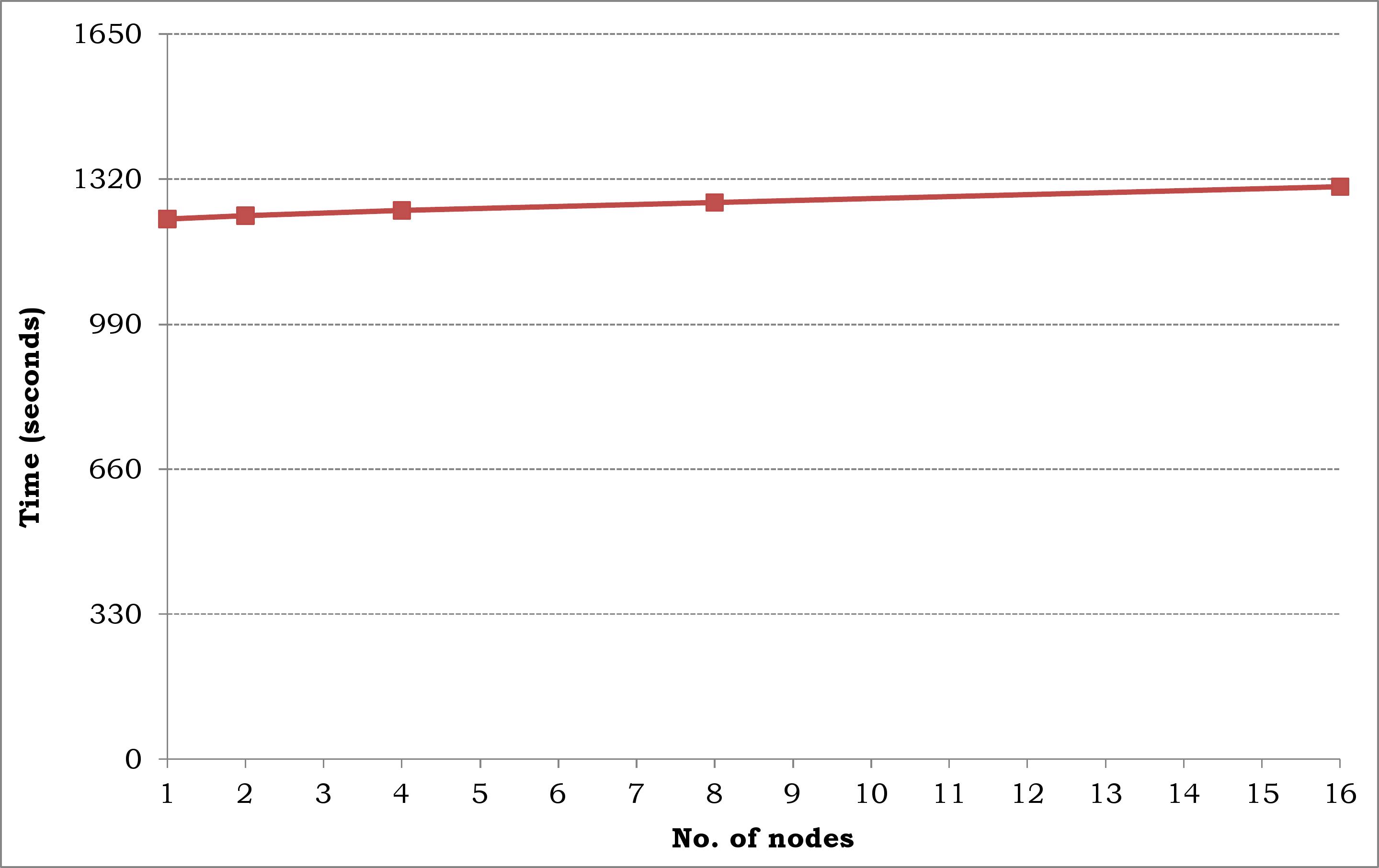
Figure 4: Running time of QuPARA on an increasing number of nodes with a fixed number of layers per job and one job per node

Figure 5 shows the increase in running time when the number of layers is increased from 200 to 3200 while keeping the number of nodes fixed. Once again, each layer covered 5 ELTs, the YET contains 1,000,000 trials, each consisting of 1,000 events. 16 nodes were used in this experiment. As expected, the running time of QuPARA increases linearly with the input size as we increase the number of layers. With the increase in the number of layers, the time taken for setup, I/O time, and the time for all numerical computations scale in a linear fashion. The time taken for building the combined ELT, by the reducer, and for clean up are a constant. For 200 Layers, only 30% of the time is taken for computations, and the remaining time accounts for system and I/O overheads. For 3200 layers, on the other hand, more than 80% of the time is spent on computations.

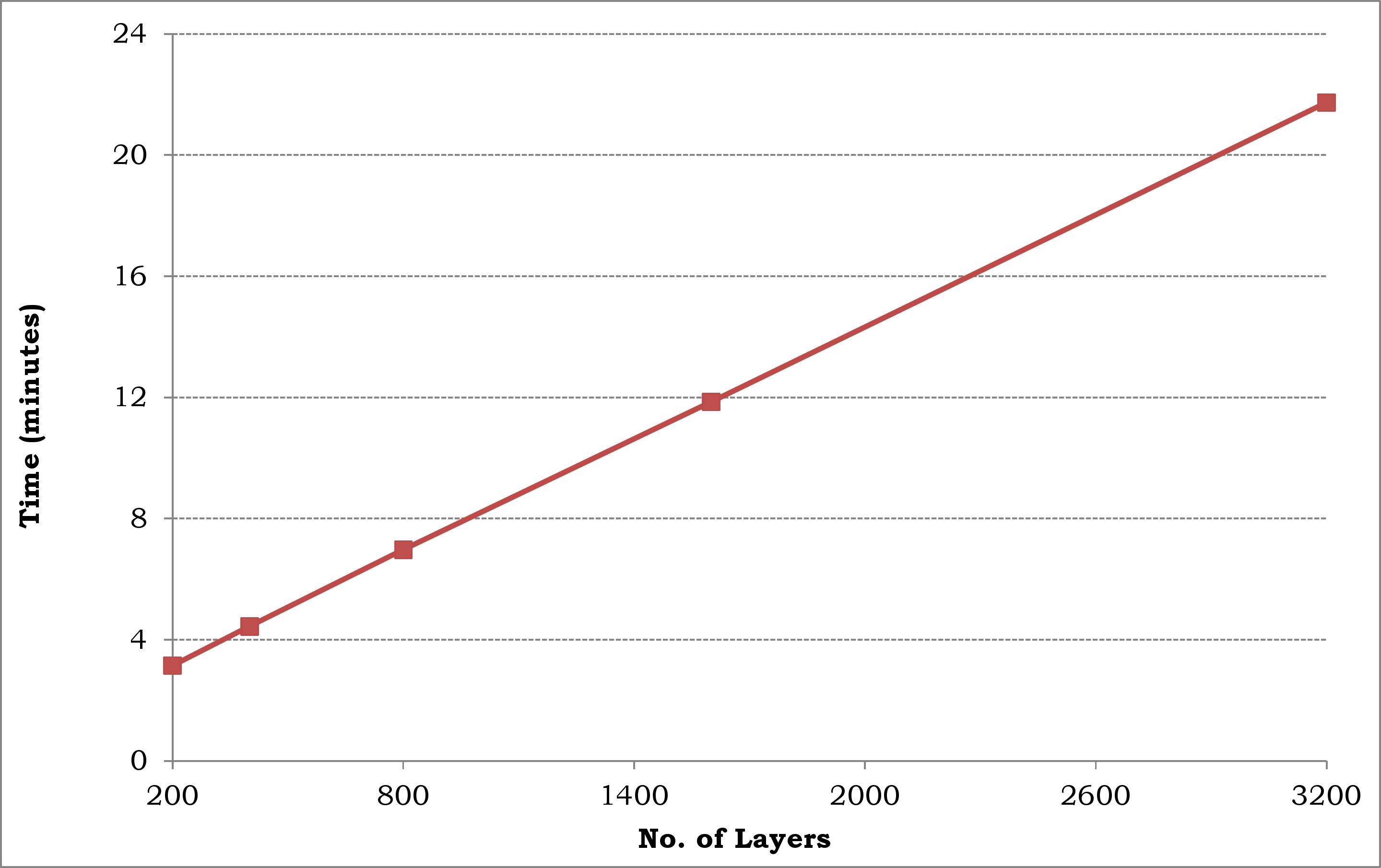
Figure 5: Running time of QuPARA on an increasing number of layers with a fixed number of nodes

Figure 6 shows the decrease in running time when the number of nodes is increased but the input size is kept fixed at 3,200 layers divided into 16 jobs of 200 layers. Figure 7 shows the relative speed-up achieved in this experiment, that is, the ratio between the running time achieved on a single node and the running time achieved on up to 16 nodes. Up to 4 nodes, the speed-up is almost linear. Beyond 4 nodes, the speed-up starts to decrease. This is not due to an increase in overhead, but since the computation times have significantly reduced after 4 nodes, the overheads start to take away a greater percent of the total time.

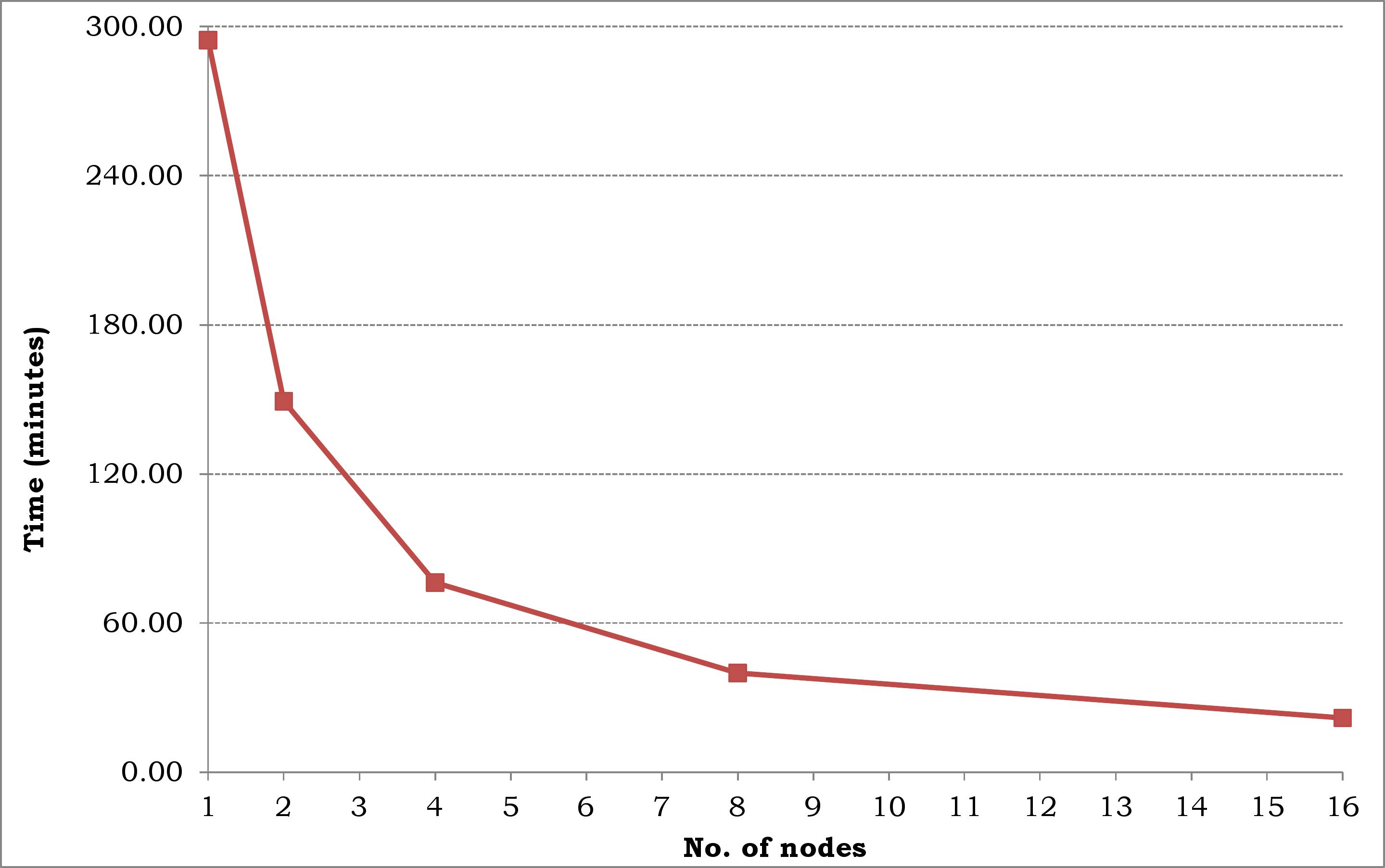
Figure 6: Running time of QuPARA on a fixed input size using between 1 and 16 nodes

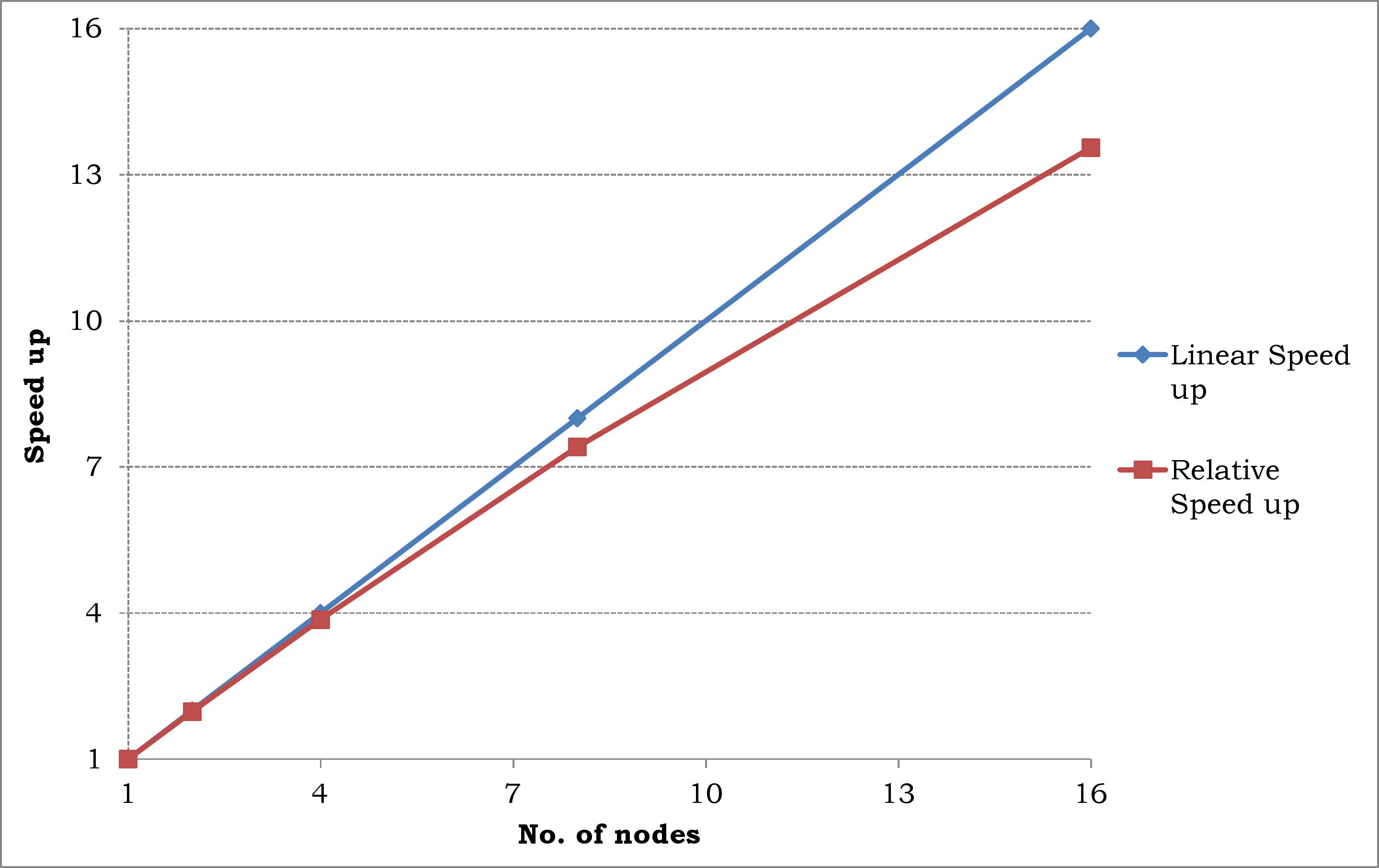
Figure 7: Speed-up achieved on the QuPARA framework

In summary, our experiments show that QuPARA is capable of performing ad-hoc aggregate risk analysis queries on industry-size data sets in a matter of minutes. Thus, it is a viable tool for analysts to carry out such analyses interactively.

VII Conclusions

Typical production systems performing aggregate risk analysis used in the industry are efficient for generating a small set of key portfolio metrics such as PML or TVAR required by rating agencies and regulatory bodies and essential for decision making. However, production systems can neither accommodate nor solve ad hoc queries that provide a better view of the multiple dimensions of risk that can impact a portfolio.

The research presented in this paper proposes a framework for portfolio risk analysis capable of expressing and solving a variety of ad hoc catastrophic risk queries, based on MapReduce, and provided a prototype implementation, QuPARA, using the Apache Hadoop implementation of the MapReduce programming model and Apache Hive for expressing ad hoc queries in an SQL-like language. Our experiments demonstrate the feasibility of answering ad hoc queries on industry-size data sets efficiently using QuPARA. As an example, a portfolio analysis on 3,200 layers and using a YET with 1,000,000 trials and 1,000 events per trial took less than 20 minutes.

Future work will aim to develop a distributed system by providing an online interface to QuPARA which can support multiple user queries.

References

- [1] R. R. Anderson and W. Dong, “Pricing Catastrophe Reinsurance with Reinstatement Provisions using a Catastrophe Model,” Casualty Actuarial Society Forum, Summer 1998, pp. 303-322.
- [2] G. G. Meyers, F. L. Klinker and D. A. Lalonde, “The Aggregation and Correlation of Reinsurance Exposure,” Casualty Actuarial Society Forum, Spring 2003, pp. 69-152.
- [3] W. Dong, H. Shah and F. Wong, “A Rational Approach to Pricing of Catastrophe Insurance,” Journal of Risk and Uncertainty, Vol. 12, 1996, pp. 201-218.
- [4] R. M. Berens, “Reinsurance Contracts with a Multi-Year Aggregate Limit,” Casualty Actuarial Society Forum, Spring 1997, pp. 289-308.
- [5] G. Woo, “Natural Catastrophe Probable Maximum Loss,” British Actuarial Journal, Vol. 8, 2002.
- [6] M. E. Wilkinson, “Estimating Probable Maximum Loss with Order Statistics,” in Casualty Actuarial Society Forum, 1982, pp. 195–209.
- [7] A. A. Gaivoronski and G. Pflug, “Value-at-Risk in Portfolio Optimization: Properties and Computational Approach,” Journal of Risk, Vol. 7, No. 2, Winter 2004-05, pp. 1–31.
- [8] P. Glasserman, P. Heidelberger, and P. Shahabuddin, “Portfolio Value-at-Risk with Heavy-Tailed Risk Factors,” Mathematical Finance, Vol. 12, No. 3, 2002, pp. 239–269.
- [9] T. White, “Hadoop: The Definitive Guide,” 1st Edition, O’Reilly Media, 2009.
- [10] Apache Hadoop Project website: \urlhttp://hadoop.apache.org/ [Last accessed: 25 May, 2013].
- [11] J. Dean and S. Ghemawat, “MapReduce: Simplified Data Processing on Large Clusters,” Communications of the ACM, Vol. 51, Issue 1, 2008, pp. 107–113.
- [12] T. Condie, N. Conway, P. Alvaro, J. M. Hellerstein, K. Elmeleegy and R. Sears, “Mapreduce Online,” EECS Department, University of California, Berkeley, Technical Report No. UCB/EECS-2009-136, October 2009. \urlhttp://www.eecs.berkeley.edu/Pubs/TechRpts/2009/EECS-2009-136.pdf [Last accessed: 25 May, 2013].
- [13] K. -H. Lee, Y. -J. Lee, H. Choi, Y. D. Chung and B. Moon, “Parallel Data Processing with MapReduce: A Survey,” SIGMOD Record Vol. 40, No. 4, 2011, pp. 11–20.
- [14] HiveQL website: http://hive.apache.org/ [Last accessed: 25 May, 2013].
- [15] E. Capriolo, D. Wampler and J. Rutherglen, “Programming Hive,” O’Reilly Media, 1st Edition, 2012.
- [16] A. Rau-Chaplin, B. Varghese and Z. Yao, “A MapReduce Framework for Analysing Portfolios of Catastrophic Risk with Secondary Uncertainty,” accepted for publication in the Workshop Proceedings of the International Conference on Computational Science, 2013.
- [17] P. Grossi and H. Kunreuter, “Catastrophe Modelling: A New Approach to Managing Risk,” Springer, 2005.
- [18] K. Shvachko, K. Hairong, S. Radia, R. Chansler, “The hadoop Distributed File System,” Proceedings of the 26th IEEE Symposium on Mass Storage Systems and Technologies, 2010, pp. 1–10.
- [19] Hadoop Distributed File System website: \urlhttp://hadoop.apache.org/docs/r1.0.4/hdfs_design.htmlS [Last accessed: 25 May, 2013]
- [20] Amazon Elastic MapReduce (Amazon EMR) website: \urlhttp://aws.amazon.com/elasticmapreduce/ [Last accessed: 25 May, 2013].
- [21] Google MapReduce website: \urlhttps://developers.google.com/appengine/docs/python/dataprocessing/overview [Last accessed: 25 May, 2013].
- [22] C. Eaton, D. Deroos, T. Deutsch, G. Lapis and P. Zikopoulos, “Understanding Big Data: Analytics for Enterprise Class Hadoop and Streaming Data,” McGraw Hill, 2012.