Non-Zeeman Circular Polarization of CO rotational lines in
SNR IC 443

Abstract

Context. We investigate non-Zeeman circular polarization and linear polarization levels of up to $1\%$ of ¹²CO spectral line emission detected in a shocked molecular clump around the supernova remnant (SNR) IC 443, with the goal of understanding the magnetic field structure in this source.

Aims. We examine our polarization results to confirm that the circular polarization signal in CO lines is caused by a conversion of linear to circular polarization, consistent with anisotropic resonant scattering. In this process background linearly polarized CO emission interacts with similar foreground molecules aligned with the ambient magnetic field and scatters at a transition frequency. The difference in phase shift between the orthogonally polarized components of this scattered emission can cause a transformation of linear to circular polarization.

Methods. We compared linear polarization maps from dust continuum, obtained with PolKa at APEX, and ¹²CO ($J=2\rightarrow 1$) and ($J=1\rightarrow 0$) from the IRAM 30-m telescope and found no consistency between the two sets of polarization maps. We then reinserted the measured circular polarization signal in the CO lines across the source to the corresponding linear polarization signal to test whether before this linear to circular polarization conversion the linear polarization vectors of the CO maps were aligned with those of the dust.

Results. After the flux correction for the two transitions of the CO spectral lines, the new polarization vectors for both CO transitions aligned with the dust polarization vectors, establishing that the non-Zeeman CO circular polarization is due to a linear to circular polarization conversion.

1 Introduction

Magnetic fields have been the subject of many theoretical and observational studies due to the role they play at different scales in astrophysics. In molecular clouds and star-forming regions magnetic fields are detected through their effect on the emission of dust particles and atomic and molecular gas species. For example, in the submillimeter regime the thermal radiation from non-spherical dust particles becomes linearly polarized in the presence of a magnetic field. This emission is polarized perpendicular to the field lines and a map of such polarization vectors therefore reveals the plane-of-the-sky orientation of the magnetic field (e.g., Hildebrand et al. 1999).

1.1 The Goldreich-Kylafis Effect

Magnetic fields can also cause molecular spectral lines to be linearly polarized by a few percent (Goldreich & Kylafis 1981). Molecules align with the ambient magnetic field and the presence of a source of anisotropy in the medium such as velocity gradients parallel or perpendicular to the magnetic field, or an external anisotropic radiation causes a population imbalance in the magnetic sub-levels, $M$. The transitions between these levels lead to the polarized $\pi$ ($\Delta$$M=0$) and $\sigma$ ($\Delta$$M=\pm 1$) radiation, the former being parallel and the latter perpendicular to the magnetic field. Depending on which sub-level population dominates, the detected linear polarization can be in either direction. This 90^∘ ambiguity can in principle be resolved by obtaining molecular line polarization maps at different transition frequencies (Cortes et al. 2005).

1.2 The Zeeman Effect

Molecular emission can also become circularly polarized through the Zeeman effect. The local magnetic field removes the energy degeneracy of the magnetic sub-levels of a molecule, potentially causing a single spectral line to split into several components. The size of this splitting is directly proportional to the strength of the magnetic field. In the case of weak fields, as is the situation in molecular clouds, a Zeeman line broadening occurs rather than a splitting, and the line-of-sight component of the field can be obtained by measuring the net circular polarization of a molecular spectral line. This is so far the only direct way to measure the strength of interstellar magnetic fields (e.g., Crutcher et al. 1993, 1999).

1.3 This work

Magnetic field measurements in the submillimeter wavelengths have mostly been limited to the few aforementioned polarimetry methods, as well as the ion-neutral line comparison technique of Houde et al. (2000a) and Li & Houde (2008) (see also Hezareh et al. 2010), but recent observations have opened new insights into physical processes stemming from the interaction between magnetic fields and interstellar material. Houde et al. (2013) reported the detection of circular polarization in ¹²CO ($J=2\rightarrow 1$) and HNCO ($N_{Ka\;Kc}$ = $1_{1,12}\rightarrow 1_{1,11}$) in Orion KL and proposed a physical model based on anisotropic resonant scattering in an effort to explain these observations. More precisely, they showed that when the orientation of the magnetic field changes in the path of propagation of linearly polarized molecular line radiation, the same species of molecules that emitted this incident background radiation will resonantly scatter these in the foreground at their transition frequency. The emerging photons will acquire a phase shift between their orthogonal scattered components that causes a transformation of linear into circular polarization. Houde et al. (2013) showed that this can readily account for the levels of circular polarization reported in their observations.

In this paper, we present the linear polarization maps of ¹²CO ($J=1\rightarrow 0$) and ($J=2\rightarrow 1$) emission and also of dust emission obtained near the western molecular edge of the shell of the supernova remnant IC 443. We also show the detection of circular polarization in both transitions of CO and quantify in our analysis the amount of conversion of linear to circular polarization and the consistency of our results with the anisotropic resonant scattering model.

We review prior studies performed on IC 443-G in §2, present our observations and data analysis in §3, the results in §4, a discussion in §5, and end with a short summary in §6.

2 Source Description

IC 443 is among the most extensively studied Galactic SNRs, located at a distance of 1.5 kpc (Fesen 1984), in the Gem OB1 association (Heiles 1984) at $\alpha\,(J2000)=06^{\mathrm{h}}18^{\mathrm{m}}02\aas@@fstack{s}7$, $\delta\,(J2000)=+22^{\circ}39^{{}^{\prime}}36^{{}^{\prime\prime}}$. IC 443 has an estimated age of 20,000 yr and reveals a non-circular morphology with two shells of different radii, namely Shell A at $7$ pc and Shell B at $13$ pc. It is suggested that the remnant initially evolved in an inhomogeneous medium and that Shell B may be a part of the remnant blown out into a rarefied medium (Lee et al. 2008). This SNR is particularly interesting because of the interaction of its so-called Shell A with the surrounding molecular cloud. The first evidence for this interaction was found in shocked OH absorption lines by DeNoyer (1979). The SNR was mapped in the $J=1\rightarrow 0$ transition of CO and HCO⁺ emission by Dickman et al. (1992), who identified eight clumps that were then labeled A to H. The clumps are arranged in a fragmentary, flattened ring with Clump G (hereafter IC 443-G) being the most massive of all at approximately $2\times 10^{3}$ M_⊙ (Xu et al. 2011), located in the westernmost edge of this ring. The correspondence of the HCO⁺ clumps with the H₂ peaks previously identified by Burton et al. (1988, 1990) was an additional sign of interaction of the SNR with its surrounding molecular cloud.

The physics of the shocked gas within Clump G is modeled as a tilted molecular ring, with the shock transverse to the line of sight (Dickman et al. 1992; van Dishoeck et al. 1993). However, it has been suggested that in this clump, a mixture of both J-type and C-type shocks rather than a single shock model can satisfyingly account for the observations (Burton et al. 1990; Wang & Scoville 1992).

Besides the extensive multi-wavelength studies of the SNR structure and the physical parameters of the molecular clumps associated with it, the magnetic field in this source has also been explored to some degree. Characterizing the direction of the magnetic field with respect to the structure of the shocks is important to constrain multi-dimensional models of such regions, as illustrated in the shock studies of Kristensen et al. (2008) and Gustafsson et al. (2010) in the context of similar molecular shocks associated with star formation processes. Wood et al. (1991) performed polarization observations of the filamentary structure of the northeast edge of IC 443 at $6$ cm with the Very Large Array (VLA) and found a correlation between the strength of the field with regions of relatively high polarized intensity, but the direction of the mean field in those regions was on average oriented neither parallel nor perpendicular with respect to the rim. Claussen et al. (1997) performed a high resolution search in the SNR for OH maser lines at 1720.53 MHz and found a total of six maser spots, all within IC 443-G. Masing lines of OH at this frequency typically arise in the molecular gas behind a slow, non-dissociative shock (Lockett et al. 1999). Although no estimate was obtained for the line-of-sight component of the magnetic field, the discovery of OH (1720 MHz) masers associated with the shocked molecular gas supports the idea that the shock is propagating into a dense magnetized molecular gas. Koo et al. (2010) measured the Zeeman splitting of the H I 21 cm emission line from shocked atomic gas in IC 443 and derived an upper limit of 100-150 $\mu$G on the strength of the line-of-sight field component, which is considerably smaller than the field strengths expected from a strongly shocked dense cloud. They concluded that either the magnetic field within the telescope beam is mostly randomly oriented or the high-velocity H I emission is from a shocked interclump medium of relatively low density. In the most recent radio continuum polarization survey at 6 cm, Gao et al. (2011) found the magnetic field around the SNR dipole-shaped with the configuration being radial around the north eastern rim. To our knowledge there has been no published higher resolution studies at shorter wavelengths on mapping the magnetic field in this source and this is what we accomplish in this work.

3 Observations and Data Processing

3.1 IRAM 30-m Observations

We obtained on-the-fly maps of CO ($J=1\rightarrow 0$) at 115.271 GHz and CO ($J=2\rightarrow 1$) at 230.538 GHz in decent weather conditions ($0.08<\tau_{225}<0.12$) in IC 443-G between 2012 January 6 and 10 with the IRAM 30-m telescope on Pico Veleta, in the Spanish Sierra Nevada. We used the EMIR receiver (Carter et al. 2012), which is equipped with four dual-polarization spectral bands, each with orthogonal linearly polarized feed horns. Since EMIR allows for dual band observations with certain band configurations, we used the E0/E2 combination centered at 90 GHz and 230 GHz, respectively, to map the two transitions of CO simultaneously in the upper sideband of the double-sideband receiver system. We used the XPOL polarimeter, a special configuration of the digital correlator backend VESPA, (Thum et al. 2008) for the polarization measurements. The Stokes parameters relate to the time-averaged horizontal ($E_{x}$) and vertical ($E_{y}$) electric fields from the receiver horns and their relative phase difference $\phi$ as follows

$$\begin{array}[]{ccc}I&=&\langle\,E^{2}_{x}\,\rangle+\langle\,E^{2}_{y}\,\rangle\\ \\ Q&=&\langle\,E^{2}_{x}\,\rangle-\langle\,E^{2}_{y}\,\rangle\\ \\ U&=&2\langle\,E_{x}\,E_{y}\,\mathrm{cos}\,\phi\,\rangle\\ \\ V&=&2\langle\,E_{x}\,E_{y}\,\mathrm{sin}\,\phi\,\rangle.\\ \end{array}$$ (1)

As the above equations imply, the Stokes $I$ and $Q$ are calculated from total power measurements while Stokes $U$ and $V$ are obtained through the cross-correlation of the IF signals. All Stokes parameters are obtained in the Nasmyth reference frame, from where they are transformed to the equatorial reference frame following the IAU definition. In this convention, polarization angles increase counter-clockwise from sky north, and the sign of Stokes $V$ is determined from $V=E^{2}_{\mathrm{RHC}}-E^{2}_{\mathrm{LHC}}$, where RHC (LHC) is the right (left)-handed circular polarization, with its electric field vector rotating counter-clockwise (clockwise) as seen by the observer.

For the two frequency bands E2 and E0, the average line-of-sight system temperatures were 155 K and 224 K leading to typical antenna temperature noise of 80 and 100 mK in a resolution bandwidth of 156 KHz, respectively. XPOL was configured with a channel spacing of 156.25 kHz, covering a bandwidth of 53 and 105 MHz for the CO ($J=1\rightarrow 0$) and ($J=2\rightarrow 1$) transitions, respectively. We obtained 24 on-the-fly maps with a size of $200^{\prime\prime}\times 140^{\prime\prime}$ at reference coordinates $\alpha(J2000)=06^{\mathrm{h}}16^{\mathrm{m}}42\aas@@fstack{s}21$, $\delta(J2000)=22^{\circ}31^{\prime}23\aas@@fstack{\prime\prime}6$ at a position angle of $17^{\circ}$ (measured eastward from sky North) in pairs of orthogonal scanning modes. Taking into account temperature and phase calibrations and off-source reference measurements, the observing time to complete a pair of maps was about 45 minutes. We also obtained OTF maps of Mercury on 2012 February 10 to determine the instrumental polarization mainly caused by the spurious conversion from Stokes $I$ into the Stokes parameters $Q$, $U$ and $V$, and to characterize the polarization in the side-lobes of the telescope beam. Every pair of OTF maps of the planet took about 10 minutes to complete, and the observations were performed with the required continuum sensitivity as total-power OTF maps, with 280 and 520 MHz bandwidths and spatial resolutions of $21\aas@@fstack{\prime\prime}3$ and $10\aas@@fstack{\prime\prime}7$ to match the CO ($J=1\rightarrow 0$) and ($J=2\rightarrow 1$) map resolutions, respectively.

3.2 IRAM 30-m Data Calibration

A very important step in obtaining the Stokes parameters involves the calibration of temperature and phase during the observations. Temperature calibration on the signals from the two orthogonal EMIR receivers are performed using the traditional hot/cold load technique, i.e., taking subscans on the sky, an ambient (hot) load, and a cold load. For phase calibration, one has to correct for the optical and electronic delays, from the aperture plane of the telescope all the way to the analog-to-digital converter of the correlator. These delays are different for the orthogonally linearly polarized components of the incoming radiation field and therefore modify their intrinsic phase difference, $\phi$. This instrumental phase shift occurring between the temperature calibration unit in the Nasmyth cabin and the correlator is measured with a wire grid introduced into the beam in front of the cold load of the calibration unit (Thum et al. 2008). The calibration procedure is performed before starting every OTF map and takes about a minute to complete. the XPOL calibration software also determines the sign of the Stokes parameters in agreement with the IAU convention.

3.3 IRAM 30-m Data processing and correction for instrumental effects

The data reduction software was developed using the GILDAS package. The CO spectral lines in both transitions span a wide range of velocities, from about $-30$ to $20$ km s^-1 with the broad line wings implying that the spectra arise from the shocked gas. A self-absorption feature is seen in the velocity range of about $-7$ to $-2$ km s^-1 in the spectra and we therefore created data cubes for the Stokes parameters as well as the fractional polarization levels, by integrating the relevant parameters across the blue- and red-shifted wings separately to avoid the self-absorption dip and also to investigate the polarization pattern across the different velocity ranges.

The next crucial step was to remove the spurious polarization signal from the Stokes maps of CO. The response of an ideal receiver, i.e., without any spurious polarization or unwanted mixing of the Stokes parameters, obeys the following set of equations ($*$ denotes the convolution product)

$$S_{\rm i,obs}=B_{\rm i,sky}*P_{0},\hskip 56.9055pti=0,1,2,3$$ (2)

where $S_{\rm i,obs}$ is the measured flux density with the indices $i=0$ to 3 refering to the Stokes parameters $I$, $Q$, $U$ and $V$, respectively, as a function of $B_{\rm i,sky}$ the sky brightness distribution in the corresponding Stokes parameter and $P_{0}$ the total power beam. However, the devices in the path along which the radiation is propagating, i.e., horns, beam splitters, the reflector and sub-reflector and other mirrors, can excite electromagnetic modes of which the net polarization is non-vanishing. The deviation of the Stokes beams from the total power beam pattern $P_{0}$ is mainly caused by the misalignment between the orthogonally polarized horns and also by the optical elements in the warm and cold optics (e.g., elliptical mirrors), and to a lesser degree from non-optimal illumination of the sub-reflector by the invidual horns. The former leads to Stokes beams that are invariable with respect to changes in elevation and parallactic angles in the Nasmyth focus of the telescope, while the latter adds a higher order elevation dependence.

As mentioned above, the main source of instrumental polarization in the observations is the leakage of the signal in the Stokes $I$ into the other Stokes parameters. A higher order effect is the spurious conversion among the other Stokes parameters. Since Stokes $Q$ is obtained through auto-correlations while $U$ and $V$ are calculated through cross-correlations, the exchange of flux between Stokes $Q$ and the latter two in the Nasmyth cabin is negligible. But after the rotation of the Stokes $Q$ and $U$ to the sky reference frame, there will be some mixing between these parameters that may affect the accuracy of the polarization angles. The latter, however, depends mainly on the orientation of the calibration grid in the telescope cabin, which has been measured with a precision of $0.5^{\circ}$ (Thum et al. 2008). The polarization angle calibrations on the Crab nebula (Aumont et al. 2010) and further tests using SiO masers (Thum et al. 2008) show that contributions from receiver noise and instrumental polarization signals affect the angle calibrations more strongly than the rotation of the Stokes parameters to the Equatorial frame.

The spurious power exchange between Stokes $U$ and $V$ happens due to the residual error in the phase calibration. We can express the observed Stokes $U$ in terms of the intrinsic Stokes $U$ and $V$ as

$$U_{obs}=U_{int}-V_{int}\,\Delta\phi,$$ (3)

where $\Delta\phi$ is the residual phase error (to the first order). From earlier polarization measurements at the IRAM 30-m on the Crab Nebula, $\Delta\phi$ was measured to be 0.02 radians across an $11^{\prime\prime}$ beam (Wiesemeyer et al. 2011). Therefore, even for comparable intrinsic Stokes $U$ and $V$ in a measurement, the power leakage from $U$ to $V$ is about $2\%$ of the intrinsic $V$, which is negligible.

In light of the aforementioned sources of spurious polarization signals we express the equations for our Stokes $Q$, $U$ and $V$ measurements with

$$S_{\rm i,obs}=B_{\rm i,sky}*P_{0}+B_{\rm 0,sky}*P_{\rm i}$$ (4)

for $i=1,2,3$, respectively. The second term in the above equation describes the leakage from Stokes $I$ into the other parameters. The instrumental response functions $P_{\rm i}$ can be measured on a strong and unpolarized source, such as Mercury. However, the phase effect of the planet could lead to a residual linear polarization even in spatially unresolved observations (Greve et al. 2009). We avoided this issue by carrying out the observations when the planet was almost in its full phase (0.995) and as compact as $\Theta_{\mathrm{M}}=4\aas@@fstack{\prime\prime}9$, i.e., spatially unresolved even in the $10\aas@@fstack{\prime\prime}7$ beam of the CO ($J=2\rightarrow 1$) data. The Stokes maps of Mercury may be represented as

$$S_{\rm i,\mathrm{M}}=B_{\rm 0,\mathrm{M}}*P_{\rm i},$$ (5)

where $B_{\rm 0,\mathrm{M}}$ is Mercury’s intrinsic brightness distribution approximated by a disk whose constant surface intensity is normalized to unity. We define the function $G$, such that $G=B_{0,\mathrm{M}}*P_{0}$ and approximate it as a Gaussian with a full-width-half-maximum (FWHM) of

$$\Theta=\sqrt{\Theta_{\mbox{\sc fwhm}}^{2}+\frac{\ln{2}}{2}\Theta_{\mathrm{M}}^{2}},$$ (6)

where $\Theta_{\mbox{\sc fwhm}}^{2}$ is the width of the telescope beam $P_{0}$. The FWHM of this Gaussian function is $21\aas@@fstack{\prime\prime}5$ for the CO ($J=1\rightarrow 0$) maps and $11\aas@@fstack{\prime\prime}1$ for the CO ($J=2\rightarrow 1$) maps. We convolve this Gaussian function with the images from Equation (4) to obtain

$$S_{\rm i,obs}*G=B_{\rm i,sky}*P_{0}*G+S_{\rm 0,obs}*S_{\rm i,\mathrm{M}},$$ (7)

where the second term from the right, $S_{\rm 0,obs}*S_{\rm i,\mathrm{M}}$, is the convolution of Stokes $I$ map of IC 443-G with each of the Stokes maps of Mercury and is our model for the instrumental polarization. We subtract these convolution products from the corresponding Stokes maps of our target (the left hand side of Equation (7)) to obtain images of the instrinsic sky brightness distribution of the Stokes parameters $Q$, $U$ and $V$ (Equation (2)) but with degraded spatial resolutions of $30\aas@@fstack{\prime\prime}3$ and $15\aas@@fstack{\prime\prime}4$ for the CO ($J=1\rightarrow 0$) and ($J=2\rightarrow 1$) transitions, respectively. Finally, the reduced maps were deconvolved to the original resolutions of the respective CO beams.

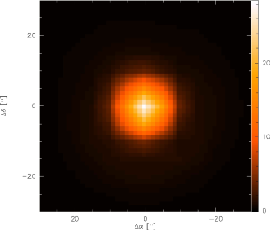
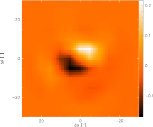
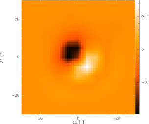
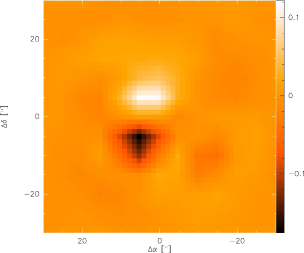
Figure 1: Starting from top left, going clockwise are the intensity maps of Mercury in Stokes $I$, $Q$, $U$, and $V$ at $1.3$ mm. The color wedge on the right vertical scale of the figures has units of Jy/beam and the maps are over-sampled by a factor of 4 for better display.

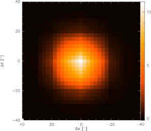
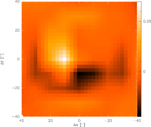
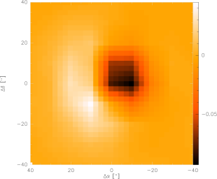
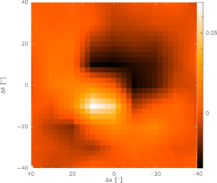
Figure 2: Same order of maps as in Figure 1 are the intensity maps of Mercury in Stokes $I$, $Q$, $U$, and $V$ at $3$ mm. These maps are also over-sampled by a factor of 4 for better display.

Figure 1 shows the Stokes maps for Mercury at 1 mm while Figure 2 shows the Stokes maps at 3 mm. The Stokes maps of Mercury are over-sampled by a factor of four for better display purposes. The amount of instrumental polarization that we measured towards Mercury on the optical axis were $Q/I=0.2$ %, $U/I=0.09$ % and $V/I=0.5$ % at 1 mm, with the side-lobes reaching $1.2\%$ in the reference frame of the Nasmyth focus. The corresponding polarization levels at 3 mm were $Q/I=0.1$ %, $U/I=0.02$ % and $V/I=0.6$ % on the optical axis and $0.8\%$ in the side-lobes.

In order to subtract the instrumental polarization from the data correctly, we had to rotate the Stokes maps of Mercury, which are invariable in the Nasmyth reference frame, to the same elevation and parallactic angles of the IC 443-G maps in the plane of the sky:

$$\begin{array}[]{ccc}\Delta\alpha_{\mathrm{IC\,443-G}}&=&\Delta\alpha_{\mathrm{M}}\,\mathrm{cos}(\Delta\gamma)+\Delta\delta_{\mathrm{M}}\,\mathrm{sin}(\Delta\gamma)\\ \\ \Delta\delta_{\mathrm{IC\,443-G}}&=&-\Delta\alpha_{\mathrm{M}}\,\mathrm{sin}(\Delta\gamma)+\Delta\delta_{\mathrm{M}}\,\mathrm{cos}(\Delta\gamma).\end{array}$$ (8)

Here $\Delta\alpha$ and $\Delta\delta$ are the coordinate offsets from the map center, $\Delta\gamma=\gamma_{\mathrm{M}}-\gamma_{\mathrm{IC\,443-G}}$, where $\gamma=\epsilon-\eta$, with $\epsilon$ the elevation and $\eta$ the parallactic angle of the sources. The Stokes $Q$ and $U$ of each source was transformed from the Nasmyth reference frame to the equatorial reference frame with the aforementioned IAU definition of $Q$ and $U$ as

$$\begin{array}[]{ccc}Q_{\mathrm{eq}}&=&-Q_{\mathrm{N}}\mathrm{cos}(2\gamma)-U_{\mathrm{N}}\mathrm{sin}(2\gamma)\\ \\ U_{\mathrm{eq}}&=&Q_{\mathrm{N}}\mathrm{sin}(2\gamma)-U_{\mathrm{N}}\mathrm{cos}(2\gamma)\end{array}$$ (9)

In this correction algorithm, however, we assume that the instrumental Stokes $Q$ and $U$ are stationary during the OTF mapping of IC 443-G. Indeed, we examined the impact of this assumption by comparing the values for $\gamma$ recorded in every pair of OTF maps, between the beginning of the first and the end of the second map. The difference between the two $\gamma$ angles range from $3^{\circ}$ to $34^{\circ}$, or $16^{\circ}$ on average (the maximum is only reached once per day, namely, during transit). The removal of the instrumental polarization as described above yielded results that are indistinguishable within $1\sigma$ limits of the instrumental polarization levels.

3.4 APEX Observations

Besides the CO polarization observations at the IRAM 30-m telescope, we observed IC 443-G with the continuum polarimeter at the APEX telescope (Güsten et al. 2006), named PolKa after the German POLarimeter für bolometer KAmeras (Siringo et al. 2004). PolKa works in combination with LABOCA, the Large APEX Bolometer Camera (Siringo et al. 2009) and uses a reflection-type rotating half-wave plate (RHWP) that functions as the polarization modulator. The RHWP modulates the polarized component of the signal at $4$ times its angular speed. For a complete description of the design and operation of PolKa, see Siringo et al. (2004, 2012).

Continuum observations of IC 443-G were performed at 345 GHz within a bandwidth of 60 GHz in December 2011 and November 2012, for a total of 4.2 hours on-source integration time with average PWV values of $0.8$ mm, or alternatively $\tau_{225}\simeq 0.035$. We used OTF mapping in compact raster-spiral mode that produces uniform coverage maps over the size of the field of view of LABOCA ($11^{\prime}\times 11^{\prime}$, Siringo et al. 2009) and set the modulation frequency to $6.24$ Hz, safely above the typical frequencies of atmospheric fluctuations. Polarization observations at APEX are performed at the Cassegrain focus and the parallactic angle is corrected with negligible errors, via conversion from the horizontal to the equatorial frame, in the same manner as for regular LABOCA observations.

3.5 APEX Data Analysis

3.5.1 Demodulation of the Polarized Signal

The bolometer detectors at APEX are not polarization sensitive, therefore for polarization observations a linear polarizer was required in the beam path to produce an intensity modulation that would be recordable by the detectors. The modulated bolometer signal, in the two cases of horizontal (H) and vertical (V) positions of the analyzer, may be expressed as (Siringo et al. 2004)

$$\begin{array}[]{ccc}S_{\mathrm{H}}&=&\frac{1}{2}[I+Q\,\mathrm{cos}\,(4\omega t)+U\,\mathrm{sin}\,(4\omega t)]\\ \\ S_{\mathrm{V}}&=&\frac{1}{2}[I-Q\,\mathrm{cos}\,(4\omega t)-U\,\mathrm{sin}\,(4\omega t)]\end{array}$$ (10)

where $\omega$ is the angular speed of the wave-plate. After absolute calibration of the position angles of the RHWP the Stokes parameters are extracted using a generalized synchronous demodulation method, explained in more detail by Wiesemeyer et al. (in prep).

While the RHWP modulates the Stokes $Q$ and $U$ parameters at four times the angular speed, the Stokes $I$ is ideally not expected to be modulated (Equation (10)). It was noticed, however, that the bolometer signals also carry a spurious modulation proportional to the total intensity, which could be a result of standing waves in the system. This signal was harmonic and could be removed from the data by applying a Fourier filter to the data in every scan, while preserving the modulated polarization signal. The modulated signal was further reduced using a synchronous demodulation method (Siringo et al. 2004; Wiesemeyer et al. in prep).

3.5.2 Calibration of the Total Power and Linear Polarization

The calibration of Stokes $I$ was performed by observing primary and secondary flux calibrators as used for regular bolometer observations. The calibration factor, however, differs by about a factor of $2$ from the usual LABOCA calibration factor because of the $50\%$ flux loss due to the insertion of the analyzing polarizers. We estimate that the calibration is the same for the two analyzers (vertical and horizontal) within measurement errors. The polarized flux and fractional polarization levels were calibrated by observing the Crab nebula, a well established calibration source (Aumont et al. 2010) and further consistency checks where done towards OMC-1. We note that once the total power and the polarization level of the incoming signal are calibrated and the instrumental polarization characterized and subtracted from the data, there is no need to further calibrate the polarization angles, since the angles are directly calculated from the reduced values of Stokes $Q$ and $U$

$$\chi=\frac{1}{2}tan^{-1}(\frac{U}{Q}).$$ (11)

3.5.3 Instrumental Polarization

In order to evaluate the level of spurious polarization in our data we observed the planet Uranus, which can be considered as an unpolarized point source. We observed Uranus in a linear on-the-fly mode and measured an upper limit of $0.1\%$ linear polarization towards the center of the planet’s disk. However, the polarization level around the edges is as high as $3\%$ and is a result of weak Stokes $I$ flux and contribution to $Q$ and $U$ from the side-lobes. The Stokes maps of Uranus were convolved with the maps of IC 443-G via a similar method as explained for the IRAM 30-m data (§3.3) to account for the effect of the polarized side-lobes on the polarization data.

4 Results

4.1 Linear polarization maps of CO

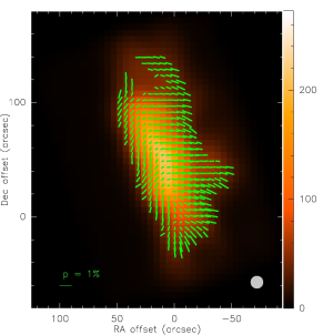
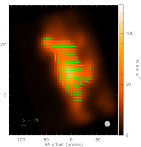
Figure 3: The polarization maps of CO ($J=2\rightarrow 1$) spectral lines in the blue-shifted ($-30$ to $-7$ km s^-1, left) and red-shifted ($-2$ to $20$ km s^-1, right) wings, with quarter-beam sampling. For each spectral line, the linear polarization levels and angles are calculated across velocity ranges spanning each line wing separately and only polarization vectors with $p\geq 3\sigma_{p}$ are plotted. These maps are corrected for instrumental polarization and the intrinsic linear polarization levels vary between $0.5-0.8\%$ across the maps. The beam size is shown in the lower right corners and the offsets are with respect to the reference coordinates $\alpha\,(J2000)=06^{\mathrm{h}}18^{\mathrm{m}}02\aas@@fstack{s}7$, $\delta\,(J2000)=+22^{\circ}39^{{}^{\prime}}36^{{}^{\prime\prime}}$.

The linear polarization map corresponding to the blue-shifted line wings of CO ($J=2\rightarrow 1$) in IC 443-G is displayed in the left panel of Figure 3 and that of the red-shifted wings is plotted in the right panel. The polarization level and angle for every given pixel are averaged over a velocity range of $-30$ to $-7$ km s^-1 for the blue-shifted wing and $-2$ to $20$ km s^-1 for the red shifted wing. This way the self-absorption dip spanning the velocity range of $-7$ to $-2$ km s^-1 is avoided in the polarization calculations. The instrumental polarization is removed from both maps and the polarization vectors are displayed for pixels with $p\geq 3\sigma_{p}$, where $p$ and $\sigma_{p}$ are the linear polarization level and its uncertainty, respectively. The Stokes $Q$ and $U$ spectra are calculated in the equatorial frame and have similar r.m.s. noise levels of $82$ mK, corresponding to an uncertainty of polarization angles $\sigma_{\chi}<9\aas@@fstack{\circ}5$. With similar polarization uncertainty values, the polarization maps for the CO ($J=1\rightarrow 0$) emission are presented in Figure 4.

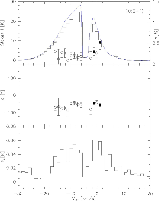
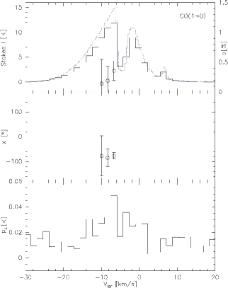
Figure 5: The linear polarization profiles for ¹²CO ($J=2\rightarrow 1$) (left) and ($J=1\rightarrow 0$) (right). The top panels show Stokes $I$ spectra at the peak position of ¹²CO emission in IC 443-G, i.e., at offsets ($20^{\prime\prime}$, $60^{\prime\prime}$) from the map origin ($\alpha\,(J2000)=06^{\mathrm{h}}18^{\mathrm{m}}02\aas@@fstack{s}7$, $\delta\,(J2000)=+22^{\circ}39^{{}^{\prime}}36^{{}^{\prime\prime}}$), overlaid with fractional linear polarization levels $p$ smoothed to 1.2 km s^-1 and 1.4 km s^-1, respectively. The dashed profiles are Stokes $I$ at the original resolution of 0.2 km s^-1 and 0.4 km s^-1 for the higher and lower transitions, respectively. The corresponding polarization angles ($\chi$) are plotted in the middle panel and the linear polarization ($p_{\mathrm{L}}=\sqrt{Q^{2}+U^{2}}$) intensity profiles across the spectral line in the bottom. These spectra are corrected for instrumental polarization but not for positive bias due to noise.

For a more detailed view of the linear polarization behaviour across a spectral line, Figure 5 presents sample linear polarization profiles of the CO ($J=2\rightarrow 1$) and ($J=1\rightarrow 0$) spectral lines at the peak position of CO emission at offsets ($20^{\prime\prime}$, $60^{\prime\prime}$) from the reference coordinates. The Stokes $I$ spectra are plotted on the top panels with the fractional linear polarization levels, with CO ($J=2\rightarrow 1$) smoothed to a resolution of $1.2$ km s^-1 and CO ($J=1\rightarrow 0$) to $1.4$ km s^-1. The dashed profiles are the Stokes $I$ spectra with original resolution of $0.2$ km s^-1 for CO ($J=2\rightarrow 1$) and $0.4$ km s^-1 for CO ($J=1\rightarrow 0$). The interaction of the SNR shock with the cloud is evident from the broadened wings of the spectral lines in both transitions. The filled circles show fractional linear polarization levels with $p\geq 3\sigma_{p}$ while the empty circles represent polarization levels with $P+2\sigma_{p}\leq 1\%$. The polarization angles $\chi$ corresponding to the aforementioned fractional polarization levels are shown in the middle panels. Although these spectra show a relatively small number of polarization measurements with $p\geq 3\sigma_{p}$ at the corresponding velocity resolutions, this criterion is easily met when the signals are integrated over the larger velocity ranges used for the maps in Figures 3 and 4. Finally, the linear polarization profiles, $p_{L}=\sqrt{Q^{2}+U^{2}}$, are plotted in the bottom panels. No positive noise bias correction is applied to these profiles and the data are plotted without correction for telescope efficiency. The linear polarization signals measured for the two CO transitions are consistent with what is expected from the Goldreich-Kylafis effect (Goldreich & Kylafis 1981).

4.2 Circular Polarization in CO Spectral lines

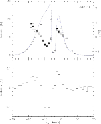
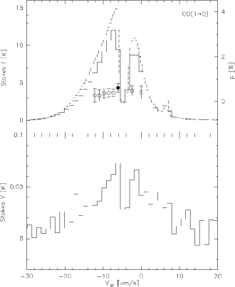
Figure 6: The circular polarization profiles for ¹²CO ($J=2\rightarrow 1$) (left) and ($J=1\rightarrow 0$) (right). The Stokes $I$ spectra at offsets ($20^{\prime\prime}$, $60^{\prime\prime}$) from the map origin ($\alpha\,(J2000)=06^{\mathrm{h}}18^{\mathrm{m}}02\aas@@fstack{s}7$, $\delta\,(J2000)=+22^{\circ}39^{{}^{\prime}}36^{{}^{\prime\prime}}$) overlaid with the fractional circular polarization levels are shown in the top panels and the Stokes $V$ spectra corresponding to the Stokes $I$ profiles are shown in the bottom panels. These spectra are corrected for instrumental polarization.

In addition to linear polarization, we also detected levels of circular polarization in both of the CO transitions in IC 443-G, which were at times higher than the linear polarization levels. After the removal of instrumental effects from the polarization signals, we obtained intrinsic circular polarization levels of $0.5-1\%$ across the CO maps. Figure 6 shows the Stokes $I$ spectra of CO ($J=2\rightarrow 1$) and ($J=1\rightarrow 0$) overlaid with the fractional circular polarization levels in the top panels at the same position as the data displayed in Figure 5. The Stokes $V$ spectra are plotted in the bottom panels. The instrumental polarization is removed from all the displayed spectra and the systematic leakage between the different Stokes parameters (explained in §3.3) are all taken into account. Besides the higher circular polarization levels across the CO ($J=2\rightarrow 1$) line, the behavior of the Stokes $V$ profile in this transition line is very different than that of the CO ($J=1\rightarrow 0$) line although they revealed similar linear polarization profiles as seen in Figure 5.

The observed circular polarization is not related to the Zeeman effect since CO is not a Zeeman sensitive molecule. The ¹²CO molecule has a Landé factor $g^{\mathrm{CO}}_{J}=-0.269$ (Gordy & Cook 1984), which multiplied by the nuclear magneton gives an approximate Zeeman splitting factor of $0.2$ mHz $\mu$G^-1. This splitting is insignificant compared to the approximately 2 Hz $\mu$G^-1 factor at 113 and 226 GHz (Bel & Leroy 1989) of the CN molecule, which is routinely used for Zeeman measurements in molecular clouds (Crutcher et al. 1999; Hezareh & Houde 2010).

4.3 Anisotropic Resonance Scattering

The physics behind the non-Zeeman circular polarization due to anisotropic resonant scattering in molecular rotational spectral lines was first discussed by Houde et al. (2013), who performed a single pointed polarization observation on CO ($J=2\rightarrow 1$) in Orion KL at the Caltech Submillimeter Observatory (CSO) using the Four-Stokes-Parameter Spectral Line Polarimeter (FSPPol). They detected non-Zeeman circular polarization levels of up to $2\%$ for this line, comparable to the linear polarization level that Girart et al. (2004) and Hezareh & Houde (2010) had measured previously for the same line at the same offsets in the source.

The model Houde et al. (2013) proposed to explain the presence of non-Zeeman circular polarization in the spectral lines of molecules such as CO and SiO is based on the anisotropic resonant scattering of linear polarization signals incident on these molecules. More precisely, we may consider a population of such molecules aligned with the magnetic field in a cloud. The emission from these molecules can become linearly polarized due to the Goldreich-Kylafis effect, for example. Upon propagation through the cloud along our line of sight, this polarized emission becomes incident on similar species of molecules in the foreground. If the orientation of the magnetic field has changed with respect to the background, then the radiation is absorbed at a transition frequency by the foreground molecules to a virtual state and is re-emitted via anisotropic resonant scattering with a phase shift between its scattered amplitudes. The incident and scattered radiation can be written in terms of $n$-photon states polarized parallel and perpendicular to the foreground magnetic field projected in the plane of the sky as (Houde et al. 2013)

$$\begin{array}[]{ccc}\left|\,\psi\right\rangle&=&\alpha\left|\,n_{\|}\right\rangle+\beta\left|\,n_{\bot}\right\rangle\\ \\ \left|\,\psi^{\prime}\right\rangle&\simeq&\alpha\,e^{i\phi}\left|\,n_{\|}\right\rangle+\beta\left|\,n_{\bot}\right\rangle,\end{array}$$ (12)

where $\phi$ is the phase shift between the aforementioned scattered components and $\theta$ the polarization angle of the incident radiation with respect to the foreground field ($\alpha=\mathrm{cos}\,(\theta)$ and $\beta=\mathrm{sin}\,(\theta)$). We can further define $n$-photon linear polarization states at $\pm 45^{\circ}$ from the field and also circular polarization states, respectively, with

$$\begin{array}[]{ccc}\left|\,n_{\pm 45}\right\rangle=\frac{1}{\sqrt{2}}(\left|\,n_{\|}\right\rangle\pm\left|\,n_{\bot}\right\rangle)\\ \\ \left|\,n_{\pm}\right\rangle=\frac{1}{\sqrt{2}}(\left|\,n_{\|}\right\rangle\pm i\left|\,n_{\bot}\right\rangle),\end{array}$$ (13)

where $\left|\,n_{+}\right\rangle\,(\left|\,n_{-}\right\rangle)$ represents the left (right) handed circular polarization state. Since the commissioning of XPOL, the polarization measurements at the IRAM telescope follow the IAU definition (Thum et al. 2008). We adopt this convention and use the aforementioned states in Equation (13) to express the Stokes parameters as

$$\begin{array}[]{l}I\,\,=\|\,\langle\,n_{\|}\left|\,\psi^{\prime}\right\rangle\|^{2}+\|\,\langle\,n_{\bot}\left|\,\psi^{\prime}\right\rangle\|^{2}=\alpha^{2}+\beta^{2}\\ \\ Q=\|\,\langle\,n_{\|}\left|\,\psi^{\prime}\right\rangle\|^{2}-\|\,\langle\,n_{\bot}\left|\,\psi^{\prime}\right\rangle\|^{2}=\alpha^{2}-\beta^{2}\\ \\ U=\|\,\langle\,n_{+45}\left|\,\psi^{\prime}\right\rangle\|^{2}-\|\,\langle\,n_{-45}\left|\,\psi^{\prime}\right\rangle\|^{2}=2\alpha\beta\,\mathrm{cos}\,(\phi)\\ \\ V=\|\,\langle\,n_{-}\left|\,\psi^{\prime}\right\rangle\|^{2}-\|\,\langle\,n_{+}\left|\,\psi^{\prime}\right\rangle\|^{2}=2\alpha\beta\,\mathrm{sin}\,(\phi).\\ \end{array}$$ (14)

The above equations show that it is the Stokes $U$ in this specific reference frame that converts to Stokes $V$ to produce circular polarization, while Stokes $Q$ and the total amount of polarization remain unaltered. However, in the absence of anisotropic resonant scattering and therefore any phase shift $\phi$ between the amplitudes of the linearly polarized radiation, Stokes $V$ will be zero and the linear polarization state of the propagating emission remains unchanged.

In order to confirm wether it is a conversion of linear to circular polarization that gives rise to the observed levels of circular polarization in our data, we first needed to obtain a dust polarization map of IC 443-G to compare with the CO polarization maps. We expect the dust polarization vectors to be perpendicular to the magnetic field lines, while those of CO have the 90^∘ ambiguity relative to the magnetic field direction in the absence of any transformation in the linear polarization states. Therefore, the CO polarization vectors are ideally expected to be either parallel or perpendicular to the dust vectors (Goldreich & Kylafis 1981).

4.4 Linear Polarization Map of Dust Emission

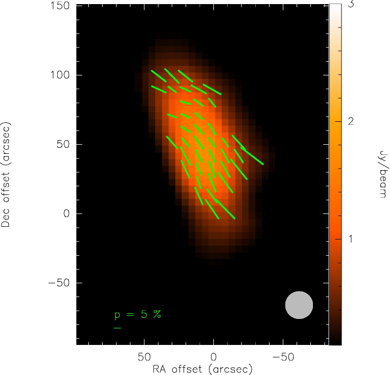
Figure 7: Dust polarization map of IC 443-G at 345 GHz with half-beam sampling obtained with PolKa at the APEX telescope. The polarization level is up to 10% and the magnetic field is oriented perpendicular to the long axis of the source. All the plotted polarization vectors have $p\geq 3\sigma_{p}$. The beam size is shown in the lower right corner and and the offsets are with respect to the reference coordinates $\alpha\,(J2000)=06^{\mathrm{h}}18^{\mathrm{m}}02\aas@@fstack{s}7$, $\delta\,(J2000)=+22^{\circ}39^{{}^{\prime}}36^{{}^{\prime\prime}}$.

The dust polarization map of IC 443-G is shown in Figure 7, where the polarization levels are measured to be up to $10\%$ and the magnetic field seems to be oriented perpendicular to the long axis of the source. All the plotted and further analyzed polarization vectors have a fractional linear polarization $p$ of at least $3\sigma_{p}$ and the uncertainty in the polarization angles is less than $10^{\circ}$.

4.5 Estimating the Magnetic Field Orientation in the Foreground

A pixel-to-pixel comparison between the dust and CO polarization maps revealed no trend of the corresponding polarization vectors being parallel or orthogonal. If the inconsistency between the dust and CO polarization maps is indeed a result of the transformation from linear to circular polarization of the latter, then a reverse transformation of these signals in the appropriate reference frame should recover the original alignment (parallel or perpendicular) between the dust and CO polarization vectors.

The first problem is obviously the determination of the orientation of the foreground magnetic field and distinguishing it from the background field in this source based on the observations. Our dust polarization map portrays the field orientation associated with IC 443-G. The CO emission in our maps originates from the shocked gas, also within the clump but it is not clear where in the cloud the magnetic field changes its orientation.

Given the lack of such information, we performed an experiment to determine whether there is a unique direction for the magnetic field that aligns with the CO molecules in the foreground and gives rise to the measured phase shift of the orthogonal components of the detected CO emission. For this purpose, at every pixel of a linear polarization map of CO, we rotated the reference frame of the Stokes $Q$ and $U$, i.e. the equatorial reference frame, from $0^{\circ}$ to $180^{\circ}$ by $5^{\circ}$ steps and calculated these Stokes parameters, $Q_{\theta}$ and $U_{\theta}$, in the new frame rotated by angle $\theta$. The corresponding Stokes $V$ for each pixel was then added to the Stokes $U_{\theta}$, conserving the signs of both parameters via

$$U^{\prime}_{\theta}=U_{\theta}\,\mathrm{cos}\,\phi+V\,\mathrm{sin}\,\phi,$$ (15)

where $\phi=\mathrm{tan^{-1}}(V/U_{\theta})$. The $Q_{\theta}$ and $U^{\prime}_{\theta}$ parameters where then rotated back to the sky coordinates and used to obtain new polarization levels and angles.

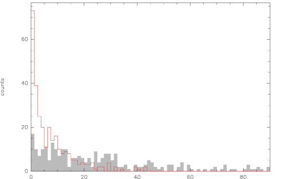
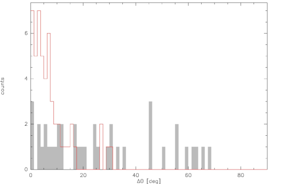
Figure 8: (Top): Histograms showing the difference between the polarization angles of dust and CO ($J=2\rightarrow 1$) maps. The grey histogram is a result of comparing the polarization map in Figure 3 (left) with that of Figure 7. In the red histogram the Stokes $V$-corrected CO ($J=2\rightarrow 1$) polarization map of Figure 9 is compared to the dust polarization map. The clear alignment of the polarization vectors of the two different tracers in the red histogram is strong evidence for a conversion of linear to circular polarization. (Bottom): Similar histograms for the comparison of the polarization vectors of dust and CO ($J=1\rightarrow 0$) maps.

After this step we produced a histogram of the distribution of the difference between the angles of the dust and corrected CO polarization vectors with the aim of finding a peak at either $0^{\circ}$ or $90^{\circ}$. The top plot in Figure 8 shows this histogram obtained with a magnetic field orientation in the east-west direction on the sky, which yields the best agreement between the polarization angles of dust and the blue-shifted wings of CO ($J=2\rightarrow 1$) line profiles. For this field orientation, $73\%$ of the corresponding polarization vectors deviate by less than $10^{\circ}$, of which $53\%$ differ by less than $5^{\circ}$. A similar histogram for the same field orientation is shown in the bottom plot of Figure 8 on the comparison between polarization angles of dust and the CO ($J=1\rightarrow 0$) transition. Due to the lower resolution of the latter map, fewer polarization vectors were available for the statistics, although the histogram shows $76\%$ of the corresponding polarization vectors deviating by less than $10^{\circ}$, of which $47\%$ differ by less than $5^{\circ}$. The histograms for the red-shifted wings of both transitions of CO display a similar trend, showing that this flux conversion spans a wide range of velocities and that the polarization characteristics of the two CO transitions are the same in this source. This is seen by comparing the corresponding maps for the blue- and red-shifted wings in Figures 3 and 4, which display similar polarization angles for the two cases.

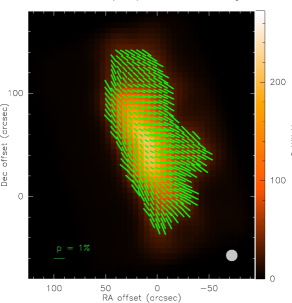
Figure 9: The polarization maps of CO ($J=2\rightarrow 1$) spectral lines in the blue-shifted (left) and red-shifted (right) wings after the conversion of the circular polarization levels into linear and re-calculation of the polarization vectors. Similar to Figures 3 and 4, only polarization vectors with $p\geq 3\sigma_{p}$ are plotted. The beam size for each map is shown in the lower right corners and the offsets are with respect to the reference coordinates $\alpha\,(J2000)=06^{\mathrm{h}}18^{\mathrm{m}}02\aas@@fstack{s}7$, $\delta\,(J2000)=+22^{\circ}39^{{}^{\prime}}36^{{}^{\prime\prime}}$.

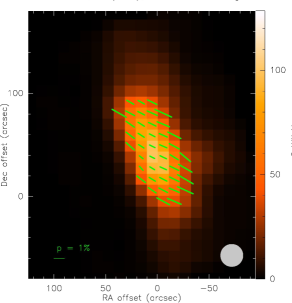
Figure 10: Same as Figure 9 but for the CO($J=1\rightarrow 0$) transition.

With the determined orientation of the foreground field (in the plane of the sky) we re-plotted the polarization maps for the blue- and red-shifted wings for both CO transitions to see what linear polarization measurements we would have obtained in the absence of polarization conversion. Figures 9 and 10 show such maps for the ($J=2\rightarrow 1$) and ($J=1\rightarrow 0$) transitions of CO, respectively. We note that not only the polarization patterns in the blue- and red-shifted wings are consistent, they are also in excellent agreement with the dust polarization map.

5 Discussion

This work follows the detection and analysis by Houde et al. (2013) of non-Zeeman circular polarization in molecular spectral lines. With the aim of studying the magnetic field structure around the interface of an SNR with an ambient molecular cloud, we produced polarization maps in both dust and CO emission in the most massive shocked clump (G) towards the western edge of the SNR IC 443 shell. We obtained both linear and circular polarization levels in the two transitions of CO and analyzed our data in several steps to confirm whether our observational results are consistent with a conversion of linear to circular polarization and the anisotropic resonant scattering model explained by Houde et al. (2013).

A very important step in the reduction of polarization data is the proper removal of instrumental effects from the observations. Polarization measurements on OTF maps of extended sources are vulnerable to significant spurious contribution from the polarized sidelobes of the telescope beam. The amount of this contribution is variable across the map, and is particularly remarkable towards the outer edges. We used a robust method of convolving our target map with Stokes maps of planet Mercury in order to account for and remove these spurious polarization signals. The intrinsic linear polarization levels of $\simeq 0.5-0.8\%$ and circular polarization levels of up to $\simeq 1\%$ that we report in CO spectral lines are therefore credible results that can be further used for more in-depth studies of the interaction between the magnetic field and cloud interface in this SNR. We note that a clear realization of this polarization conversion in the CO lines would not have been possible without this correction method for instrumental polarization.

After calibration and removal of instrumental polarization from the data, we found a unique direction for the magnetic field in the foreground gas that would provide the best alignment between dust and CO linear polarization maps after a reverse transformation of circularly polarized power into linear in the CO data. We have no further information about the foreground cloud, but we expect that it is optically thin. That is, an incident background photon cannot be absorbed by the foreground cloud but can undergo several resonant scattering events before escaping the cloud, whose thickness should therefore not (approximately) exceed the effective mean free path set by both the resonant scattering and absorption processes.

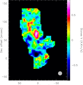
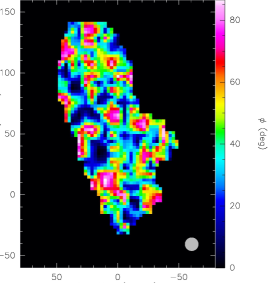
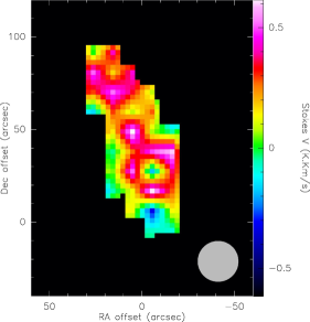
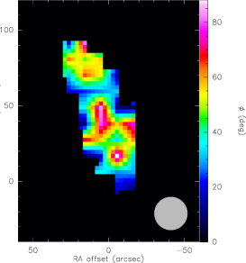
Figure 11: (Top): The map of Stokes $V$ integrated over the blue-shifted wings of the CO ($J=2\rightarrow 1$) emission in IC 443-G (left) and the corresponding $0^{\circ}$ to $90^{\circ}$ distribution of the phase-shift $\phi$ between the orthogonally polarized radiation components of CO ($J=2\rightarrow 1$) averaged over the same velocity ranges as Stokes $V$ (right). The bottom panels show the same as above but for CO ($J=1\rightarrow 0$). The beam sizes are shown in the lower right corners and the offsets are with respect to the reference coordinates $\alpha\,(J2000)=06^{\mathrm{h}}18^{\mathrm{m}}02\aas@@fstack{s}7$, $\delta\,(J2000)=+22^{\circ}39^{{}^{\prime}}36^{{}^{\prime\prime}}$.

The resulting maps for both the blue- and red-shifted line wings are very similar for the two transitions, although their polarization transformation patterns, i.e., the distribution of the phase shift $\phi$ across the source are very different. Figure 11 shows the Stokes $V$ maps integrated over the blue-shifted line wings for the two CO transitions and the corresponding maps of the phase shift $\phi$ calculated from Equation (1) using the Stokes $U$ and $V$ values integrated across the blue-shifted line wings. Although the CO ($J=1\rightarrow 0$) maps have a lower resolution compared to the higher transition, it seems that the linear to circular polarization transformation is more extended in the former. Moreover, there is no obvious correlation between the corresponding offsets in the two sets of maps affected by this polarization transformation. We therefore believe that we have obtained a correct direction for the foreground magnetic field, otherwise we would not have obtained this degree of consistency between the two sets of CO polarization maps with the dust polarization map (Figure 8) after the flux correction.

Houde et al. (2013) showed that the magnitude of $\phi$ is proportional to several physical parameters including the excitation temperature and number density of the observed species and also the square of the strength of plane-of-sky component of the magnetic field such that

$$\phi\,(\omega)\simeq\omega^{2}_{Z}\mathrm{sin}^{2}(\iota)\,\frac{3\pi\,c^{2}l^{4}_{\mathrm{mp}}A_{\mathrm{ba}}n_{\mathrm{CO}}g_{1}e^{-E_{1}/kT_{ex}}}{4\hbar\omega^{3}_{0}\omega^{2}Q_{\mathrm{CO}}(T_{\mathrm{ex}})}\sqrt{u(\omega)u^{\prime}(\omega)}\,I(\omega),$$ (16)

where $\omega_{Z}$ is the Zeeman splitting, $\iota$ the magnetic field inclination angle relative to the line of sight, $l_{\mathrm{mp}}$ the size of the region of interaction, $n_{\mathrm{CO}}$ the density of CO molecules, $A_{\mathrm{ba}}$ the spontaneous emission coefficient, $\omega$ and $\omega_{0}$ the frequencies of incident photon and the rotational transition, respectively, $u(\omega)(u^{\prime}(\omega))$ the incident (scattered) linear polarization energy density (obtained observationally from the antenna temperature), and $I(\omega)$ is an integral over the linear polarization profile for a given CO spectral line. In order to perform a more in-depth analysis on the physics of this polarization transformation and its relationship with the ambient magnetic field, we need to calculate the temperature and density profiles in this source. This analysis will be the focus of a follow-up paper.

Finally, we point out the linear polarization measurements on an OH maser line detected at 1.7 GHz by Claussen et al. (1997) in IC 443-G with the VLA. They found linear polarization in one out of six observed maser lines, with a polarization level of 4.5 % and a polarization angle of $21^{\circ}$ (no uncertainty given). The location of this OH maser line, which Hoffman et al. (2003) revisited, corresponds to offsets ($20^{\prime\prime},60^{\prime\prime}$) from our reference coordinates for IC 443-G. At that location we obtained a polarization angle of $29^{\circ}\pm 2^{\circ}$ from the (corrected) CO ($J=2\rightarrow 1$) polarization map, $32^{\circ}\pm 3^{\circ}$ from the CO ($J=1\rightarrow 0$) map, and $20^{\circ}\pm 8^{\circ}$ from our dust polarization map. Considering the uncertainties in our polarization angles, the width of the histograms of dust and CO polarization angle differences ($5^{\circ}$ for CO ($J=2\rightarrow 1$) and $8^{\circ}$ for CO ($J=1\rightarrow 0$)) in Figure 8, we find our results in good agreement with the polarization measurement of Claussen et al. (1997). These results also support their assessment that the observed OH masers indeed arise from the shocked gas within IC 443-G.

6 Summary

We measured linear polarization and also non-Zeeman circular polarization levels of up to $1\%$ in ¹²CO ($J=2\rightarrow 1$) and ($J=1\rightarrow 0$) spectral line emission observed with the IRAM 30-m telescope in a shocked molecular clump around the SNR IC 443. We also obtained a dust polarization map of this source with PolKa at the APEX telescope and compared it to the linear polarization maps of CO and found no obvious alignment between the corresponding polarization vectors, suggesting an alteration in the linear polarization state of the CO emission. We found that the detected circular polarization signal in CO lines is consistent with a physical model based on anisotropic resonant scattering introduced by Houde et al. (2013). In this model linearly polarized CO emission emerging from the background interacts with similar species of molecules aligned with the ambient magnetic field in the foreground and scatters at a transition frequency. The relative phase shift that results between the orthogonally polarized components of this scattered emission can cause a transformation of linear to circular polarization. We therefore reinserted the circular polarization signal in the CO lines across IC 443-G to the corresponding linear polarization signal to test whether before the linear to circular polarization conversion the linear polarization vectors of the CO emission were aligned with those of the dust. Indeed after the flux correction for the two transitions of the CO spectral lines, the new CO polarization vectors for both transitions aligned with the dust polarization vectors.

In a future paper we will attempt to establish that the presence of circular polarization is indeed due to the anisotropic resonant scattering model of Houde et al. (2013). If this can be established, then this technique would open the possibility to measure the magnetic field in various astronomical sources using abundant molecules such as CO, which as explained earlier, is not sensitive to the Zeeman effect.

Figure 4: Same as Figure 3 but for the CO ($J=1\rightarrow 0$) transition.

References

- Aumont et al. (2010) Aumont, J., Conversi, L., Thum, C., Wiesemeyer, H., Falgarone, E. et al. 2010, A&A, 514, 70
- Bel & Leroy (1989) Bel, N. & Leroy, B. 1989, A&A, 224, 206
- Burton et al. (1990) Burton, M. G., Hollenbach, D. J., Haas, M. R., & Erickson, E. F. 1990, ApJ, 355, 197
- Burton et al. (1988) Burton, M. G., Geballe, T. R., Brand, P. W. J. L., & Webster, A. S. 1988, MNRAS, 231, 617
- Carter et al. (2012) Carter, M., Lazareff, B., Maier, D., Chenu, J.-Y., Fontana, A.-L. et al. 2012, A&A, 538, 89
- Claussen et al. (1997) Claussen, M. J., Frail, D. A., Goss, W. M., & Gaume, R. A. 1997, ApJ, 489, 143
- Cortes et al. (2005) Cortes, P. C., Crutcher, R. M., & Watson, W. D. 2005, ApJ, 628, 780
- Crutcher et al. (1999) Crutcher, R. M., Troland, T. H., Lazareff, B., Paubert, G., & Kaze‘s, I. 1999, ApJ, 514, L121
- Crutcher et al. (1993) Crutcher, R. M., Troland, T. H., Goodman, A. A., Heiles, C., Kazes, I., & Myers, P. C. 1993, ApJ, 407, 175
- Deguchi & Watson (1984) Deguchi, S., & Watson, W. D. 1985, ApJ, 289, 621
- DeNoyer (1979) DeNoyer, L. K. 1979, ApJ, 228, 41
- Dickman et al. (1992) Dickman, R. L., Snell, R. L., Ziurys, L. M., & Huang, Y-L. 1992, 1992ApJ, 400, 203
- Fesen (1984) Fesen, R. A. 1984, ApJ, 281, 658
- Gao et al. (2011) Gao, X. Y., Han, J. L., Reich, W., Reich, P., Sun, X. H., & Xiao, L. 2011, A&A, 529, 159
- Girart et al. (2004) Girart, J. M., Greaves, J. S., Crutcher, R. M., & Lai, S.-P. 2004, Ap&SS, 292, 119
- Goldreich & Kylafis (1981) Goldreich, P., & Kylafis, N. D. 1981, ApJ, 243L, 75
- Gordy & Cook (1984) Gordy, W., & Cook, B. L. 1984, Microwave Molecular Spectroscopy (3rd ed.; New York: Wiley)
- Greve et al. (2009) Greve, A., Thum, C., Moreno, R. & Yan, N. 2009, A&A, 495, 639
- Gustafsson et al. (2010) Gustafsson, M., Ravkilde, T., Kristensen, L. E., Cabrit, S., Field, D., & Pineau Des Forêts, G. 2010, A&A, 513, 5
- Güsten et al. (2006) Güsten, R., Nyman, L. Å., Schilke, P., Menten, K., Cesarsky, C., & Booth, R. 2006, A&A, 454, 13
- Heiles (1984) Heiles, C. 1984, ApJS, 55, 585
- Hezareh & Houde (2010) Hezareh, T., & Houde, M. 2010, PASP, 122, 786
- Hezareh et al. (2010) Hezareh, T., Houde, M., McCoey, C., & Li, H. 2010, ApJ, 720, 603
- Hildebrand et al. (1999) Hildebrand, R. H., Dotson, J. L., Dowell, C. D., Schleuning, D. A., & Vaillancourt, J. E. 1999, ApJ, 516, 834
- Hoffman et al. (2003) Hoffman, I. M., Goss, W. M., Brogan, C. L., Claussen, M. J., & Richards, A. M. S. 2003, ApJ, 583, 272
- Houde et al. (2013) Houde, M., Hezareh, T., Jones, S., & Rajabi, F. 2013, ApJ, 764, 24
- Houde et al. (2000a) Houde, M., Bastien, P., Peng, R., Phillips, T. G., & Yoshida, H. 2000a, ApJ, 536, 857
- Koo et al. (2010) Koo, B-C., Heiles, C., Stanimirović, S., & Troland, T. 2010, AJ, 140, 262
- Kristensen et al. (2008) Kristensen, L. E., Ravkilde, T. L., Pineau Des Forêts, G., Cabrit, S., Field, D., Gustafsson, M., Diana, S. & Lemaire, J.-L. 2008, A&A, 477, 203
- Lee et al. (2012) Lee, J-J., Koo, B-C., Snell, R. L., Yun, M. S., Heyer, M. H., & Burton, M. G. 2012, ApJ, 749, 34
- Lee et al. (2008) Lee, J-J., Koo, B-C., Yun, M. S., Stanimirović, S., Heiles, C., & Heyer, M. 2008, AJ, 135, 796
- Li & Houde (2008) Li, H., & Houde, M. 2008, ApJ, 677, 1151
- Lockett et al. (1999) Lockett, P., Gauthier, E., & Elitzur, M. 1999, ApJ, 511, 235
- Matthews et al. (2009) Matthews, B. C., McPhee, C. A., Fissel, L. M., & Curran, R. L. 2009, ApJS, 182, 143
- Siringo et al. (2012) Siringo, G., Kovács, A., Kreysa, E., Schuller, F., Weiss, A. et al. 2012, SPIE, 8452, 06
- Siringo et al. (2009) Siringo, G., Kreysa, E., Kov/’acs, A. et al. 2009, A&A, 497, 945
- Siringo et al. (2004) Siringo, G., Kreysa, E., Reichertz, L. A., & Menten, K. M. 2004, A&A, 422, 751
- Thum et al. (2008) Thum, C., Wiesemeyer, H., Paubert, G., Navarro, S., & Morris, D. 2008, PASP, 120, 777
- van Dishoeck et al. (1993) van Dishoeck, E. F., Jansen, D. J., & Phillips, T. G. 1993, A&A, 279, 541
- Wang & Scoville (1992) Wang, Z., & Scoville, N. Z. 1992, ApJ, 386, 158
- Wiesemeyer et al. (2011) Wiesemeyer, H., Thum, C., Morris, D., Aumont, J., & Rosset, C. 2011, A&A, 528, 11
- Wiesemeyer et al. (in prep) Wiesemeyer, H., Hezareh, T., Kreysa, E. et al. 2013, PASP, in prep.
- Wood et al. (1991) Wood, C. A., Mufson, S. L., Dickel, J. R., 1991, AJ, 102, 224
- Xu et al. (2011) Xu, J-L., Wang, J-J., & Miller, M. 2011, ApJ, 727, 81