Rotation of the Trajectories of the Bright Solitons and Realignment of Intensity Distribution in the Coupled Nonlinear Schr$\rm\ddot{o}$dinger Equation

Abstract

We revisit the collisional dynamics of bright solitons in the coupled Nonlinear Schr$\rm\ddot{o}$dinger equation. We observe that apart from the intensity redistribution in the interaction of bright solitons, one also witnesses a rotation of the trajectories of bright solitons . The angle of rotation can be varied by suitably manipulating the Self-Phase Modulation (SPM) or Cross Phase Modulation (XPM) parameters.The rotation of the trajectories of the bright solitons arises due to the excess energy that is injected into the dynamical system through SPM or XPM. This extra energy not only contributes to the rotation of the trajectories, but also to the realignment of intensity distribution between the two modes. We also notice that the angular separation between the bright solitons can also manouvred suitably. The above results which exclude quantum superposition for the field vectors may have wider ramifications in nonlinear optics, Bose-Einstein condensates, Left Handed (LH) and Right Handed (RH) meta materials.

I Introduction

The potential of solitons to carry information in optical fibres which was theoretically predicted by Hasegawa and Tappert [1] in1973 was experimentally realized in 1980 by Mollenauer [2]. Since then, the propagation of temporal optical solitons in long distance optical fibre communication and optical switching devices [3] has been investigated. Mathematically speaking, the propagation of an electromagnetic wave through a single mode optical fibre when Kerr nonlinearity ( Self Phase Modulation or SPM) exactly counterbalances the group velocity dispersion is governed by the integrable ’soliton’ possessing nonlinear $Schr\rm\ddot{o}dinger$ (NLS) equation [1,3]. A single mode fiber can also support two orthogonal directions. Under ideal conditions of perfect cylindrical geometry and isotropic material, a mode excited with its polarization in one particular direction would not couple to the mode with the orthogonal state. However, in practice, small departures from cylindrical geometry or small fluctuations in material anisotropy result in mixing up of the two polarization states, thereby breaking the mode degeneracy[4]. In conventional single mode fibers, birefringence is not a constant parameter along the fiber but changes randomly because of fluctuations in the core shape and stress induced anisotropy.Thus, it is clear that when two or more optical waves co-propagate inside a fiber, they interact with each other through the fiber nonlinearity. This provides a coupling between the incident waves through the phenomenon called Cross Phase Modulation (XPM). XPM occurs because the effective refractive index of a wave depends not only on the intensity of that wave, but also on the intensity of the co-propagating wave. XPM is always accompanied by SPM. When the two waves have orthogonal polarizations, the XPM caused coupling induces a nonlinear birefringence in the fiber. Hence, the propagation of solitons through nonlinear birefringent fibres is governed by the coupled NLS equation [5] of the form,

$$iq_{1t}+q_{1xx}+2(g_{11}|q_{1}|^{2}+g_{12}|q_{2}|^{2})q_{1}=0$$ (1a)

$$iq_{2t}+q_{2xx}+2(g_{21}|q_{1}|^{2}+g_{22}|q_{2}|^{2})q_{2}=0$$ (1b)

where $q_{i}(x,t)$ (i=1,2) are the envelopes of the field components, In the above equation, $g_{11}$ and $g_{22}$ account for the strengths of self-phase modulation while $g_{12}$ and $g_{21}$ represent the strengths of cross phase modulation. It has been found that eq. (1) is integrable if either (i) $g_{11}$=$g_{12}$=$g_{21}$=$g_{22}$ or (ii) $g_{11}$=$g_{21}$=$-g_{12}$=$-g_{22}$. The first choice corresponds to the Manakov model [6,4-10] which has been investigated [7,8] and the intensity redistribution of the bright solitons has been identified. The second choice corresponds to the modified Manakov model [9,10] and its soliton dynamics has been explored. Bright solitons which are the localized solutions of coupled NLS eq.(1) continue to attract the attention of researchers even today in nonlinear optics [11] and BECs [12]. While it has been shown that soliton radiation trapping occurs due to cross phase modulation in the former case, vector soliton outcoupling occurs due to intra$/$interspecies scattering lengths in the latter case. However, it should be mentioned that since the solitons lie in the high kinetic energy regime [13], quantum superposition is forbidden.

In addition to the above physical interpretation, for handling more channels at high bit rate, it is necessary to achieve wavelength division multiplexing (WDM)[3] using coupled nonlinear schr$\rm\ddot{o}$dinger (NLS) equation through optical soliton transmission. This is possible by propagation through different channels with different carrier frequencies. In either case, two or more fields are to be propagated in the fiber. Hence, the dynamics of the fiber system is governed by the above coupled system of equations which are not integrable in general. Besides, the dynamics of a higher order coupled NLS equation including the third order dispersion, Kerr dispersion and stimulated Raman scattering has also been analyzed [14]. In addition to the above situations, coupling is also possible in the system of two parallel wave guides coupled through evanescent field overlap, the coupling of two polarization modes in uniform guides, nonlinear optical waveguide arrays and nonlinear distributed feedback structures [3]. Also, nonlinear couplers use solitons as ideal tools for performing all-optical switching operations [15].

At this juncture, it should be mentioned that the coupled NLS / coupled higher order NLS type equations discussed above have been associated with the concept of intensity redistribution of solitons, a property which has wider ramifications in optical fiber communications such as providing intensity pump sources, soliton switching [15] etc., Can one identify other properties or signatures of the coupled NLS or NLS type equations which could come in handy in the propagation of solitons in optical fibres?. The answer to this question assumes tremendous significance to improve the efficiency of soliton based communication systems. In the present paper, we unearth some new and unexplored signatures of coupled NLS equation which include the rotation of the trajectories of bright solitons, realignment of intensity distribution between the two modes and the variation of angular separation between the bright solitons. We show that all the above occurs at the expense of additional energy pumped into the dynamical system by virtue of the variation of SPM and XPM.

II Bright Solitons and their Collisional Dynamics

Invoking the constraint $g_{11}$=$g_{12}$=$g_{21}$=$g_{22}$ or $g_{11}$=$g_{21}$=$-g_{12}$=$-g_{22}$, eq.(1) can be linearized as

$$\Phi_{x} + U\Phi=0,$$ (2)

$$\Phi_{t} + V\Phi=0,$$ (3)

where $\Phi=(\phi_{1},\phi_{2},\phi_{3})^{T}$ and

$$U = \left(\begin{array}[]{ccc}-2i\zeta&\sqrt{a}\psi_{1}&\sqrt{b}\psi_{2}\\ \sqrt{a}\psi_{1}^{*}&i\zeta&0\\ \sqrt{b}\psi_{2}^{*}&0&i\zeta\\ \end{array}\right),$$ (7)

$$V = \left(\begin{array}[]{ccc}-(B+J)&A&K\\ A^{*}&B&G\\ K^{*}&H&J\\ \end{array}\right),$$ (11)

with

$$A = i\sqrt{a}\psi_{1x}+3\sqrt{a}\zeta\psi_{1},$$

$$K = i\sqrt{b}\psi_{2x}+3\sqrt{b}\zeta\psi_{2},$$

$$A^{*} = -\sqrt{a}i\psi_{1x}^{*}+3\sqrt{a}\zeta\psi_{1}^{*},$$

$$K^{*} = -\sqrt{b}i\psi_{2x}^{*}+3\sqrt{b}\zeta\psi_{2}^{*},$$

$$B = 3i\zeta^{2}+ia\psi_{1}\psi_{1}^{*},$$

$$J = 3i\zeta^{2}+ib\psi_{2}\psi_{2}^{*},$$

$$G = i\sqrt{a}\sqrt{b}\psi_{2}\psi_{1}^{*},$$

$$H = i\sqrt{a}\sqrt{b}\psi_{1}\psi_{2}^{*},$$

where, $\zeta=\mu ab$ and $\mu$ is the so called ’hidden complex isospectral parameter’ while $a$ and $b$ are real parameters. The compatibility condition $U_{t}-V_{x}+[U,V]=0$ generates the following equation

$$i\psi_{1t}+\psi_{1xx}+2(a|\psi_{1}|^{2}+b|\psi_{2}|^{2})\psi_{1}=0,$$ (12a)

$$i\psi_{2t}+\psi_{2xx}+2(a|\psi_{1}|^{2}+b|\psi_{2}|^{2})\psi_{2}=0.$$ (12b)

In the above equation, when $a$=$b$, it reduces to the Manakov model [7,8] while for $a$=$-b$, one obtains the modified Manakov model [9,10].

To generate the bright vector solitons of the above coupled nonlinear $Schr\rm\ddot{o}dinger$ eqs.(6), we now consider the vacuum solution ($\psi_{1}^{(0)}=\psi_{2}^{(0)}=0$) and employ gauge transformation approach[16] to obtain the bright soliton solutions of the following form

$$\psi_{1}^{(1)}=\varepsilon_{1}^{(1)}\beta_{1}sech(\theta_{1})e^{i(-\xi_{1})},$$ (13)

$$\psi_{2}^{(1)}=\varepsilon_{2}^{(1)}\beta_{1}sech(\theta_{1})e^{i(-\xi_{1})},$$ (14)

where

$$\theta_{1} = 2\beta_{1}x+8\alpha_{1}\beta_{1}t-2\delta_{1},$$

$$\xi_{1} = 2\alpha_{1}x+4(\alpha_{1}^{2}-\beta_{1}^{2})t-2\chi_{1},$$

with $\alpha_{1}=\alpha_{10}ab$, $\beta_{1}=\beta_{10}ab$ while $\zeta_{1}=\alpha_{1}+i\beta_{1}$ and $\bar{\zeta}_{1}=\zeta_{1}^{*}$. In the above equation, $\delta_{1}$ and $\chi_{1}$ are arbitrary parameters while $\varepsilon_{1,2}$ represent coupling parameters.

From the bright soliton solution, one understands that their amplitude not only depends on the coupling parameters $\varepsilon_{1}^{(1)}$ and $\varepsilon_{2}^{(1)}$, but also on the self-phase modulation and cross phase modulation parameters $a$ and $b$. This means that the impact of self-phase modulation and cross phase modulation can be cast suitably in the collisional dynamics of bright solitons.

To understand the impact of SPM and XPM in the coupled NLS equation, we now consider the two soliton solution obtained by employing gauge transformation approach [16] of the following form

$$\psi_{1}^{(2)}=\psi_{1}^{(1)}-2i(\zeta_{2}-\bar{\zeta_{2}})\frac{\tilde{P}_{12}}{R},$$ (15)

$$\psi_{2}^{(2)}=\psi_{2}^{(1)}-2i(\zeta_{2}-\bar{\zeta_{2}})\frac{\tilde{P}_{13}}{R},$$ (16)

where $\zeta_{2}=\bar{\zeta_{2}}=\alpha_{2}+i\beta_{2}$. The explicit forms of $\tilde{P}_{12}$ and $\tilde{P}_{13}$ are given by

$$\tilde{P}^{1}_{12}= - [M_{12}^{(1)}((\tau+\gamma M_{11}^{(1)})M_{11}^{(2)}+\gamma(M_{12}^{(1)}M_{21}^{(2)}\gamma^{*}/\tau^{2}$$

$$+ M_{13}^{(1)}M_{31}^{(2)}))+M_{32}^{(1)}((\tau+\gamma M_{11}^{(1)})M_{13}^{(2)}+\gamma(M_{12}^{(1)}$$

$$M_{23}^{(2)}+M_{13}^{(1)}M_{33}^{(2)}))\gamma^{*}/\tau^{2}+((\tau+\gamma M_{11}^{(1)})M_{12}^{(2)}$$

$$+ \gamma(M_{12}^{(1)}M_{22}^{(2)}+M_{13}^{(1)}M_{32}^{(2)}))(\tau+M_{22}^{(1)}\gamma*)/\tau^{2}],$$

$$\tilde{P}^{1}_{13}= - [M_{13}^{(1)}((\tau+\gamma M_{11}^{(1)})M_{11}^{(2)}+\gamma(M_{12}^{(1)}M_{21}^{(2)}+M_{13}^{(1)}$$

$$M_{31}^{(2)}))\gamma^{*})/\tau^{2}+M_{23}^{(1)}((\tau+\gamma M_{11}^{(1)})M_{12}^{(2)}+\gamma(M_{12}^{(1)}$$

$$M_{22}^{(2)}+M_{13}^{(1)}M_{32}^{(2)}))\gamma^{*}/\tau^{2}+((\tau+\gamma M_{11}^{(1)})M_{13}^{(2)}$$

$$+ \gamma(M_{12}^{(1)}M_{23}^{(2)}+M_{13}^{(1)}M_{33}^{(2)}))(\tau+M_{33}^{(1)}\gamma^{*})/\tau^{2}],$$

and

$$\tau = M_{11}^{(1)}+M_{22}^{(1)}+M_{33}^{(1)},\qquad\gamma=\frac{\lambda_{1}-\mu_{1}}{\mu_{2}-\lambda_{1}},$$

$$R = \tilde{P}^{1}_{11}+\tilde{P}^{1}_{22}+\tilde{P}^{1}_{33},\qquad\gamma^{*}=-\frac{\lambda_{1}-\mu_{1}}{\lambda_{2}-\mu_{1}},$$

with

$$\tilde{P}^{1}_{11} = M_{21}^{(1)}((\tau+\gamma M_{11}^{(1)})M_{12}^{(2)}+\gamma(M_{12}^{(1)}M_{22}^{(2)}+M_{13}^{(1)}$$

$$M_{32}^{(2)}))\gamma^{*}/\tau^{2}+M_{31}^{(1)}((\tau+\gamma M_{11}^{(1)})M_{13}^{(2)}+\gamma(M_{12}^{(1)}$$

$$M_{23}^{(2)}+M_{13}^{(1)}M_{33}^{(2)}))\gamma^{*}/\tau^{2}+((\tau+\gamma M_{11}^{(1)})M_{11}^{(2)}$$

$$+ \gamma(M_{12}^{(1)}M_{21}^{(2)}+M_{13}^{(1)}M_{31}^{(2)}))(\tau+M_{11}^{(1)}\gamma^{*})/\tau^{2},$$

$$\tilde{P}^{1}_{22} = M_{12}^{(1)}(\gamma M_{11}^{(2)}M_{21}^{(1)}+M_{21}^{(2)}(\tau+\gamma M_{22}^{(1)})+\gamma M_{23}^{(1)}$$

$$M_{31}^{(2)})\gamma^{*}/\tau^{2}+M_{32}^{(1)}(\gamma M_{13}^{(2)}M_{21}^{(1)}+(\tau+\gamma M_{22}^{(1)})$$

$$M_{23}^{(2)}+\gamma M_{23}^{(1)}M_{33}^{(2)})\gamma^{*}/\tau^{2}+(\gamma M_{12}^{(2)}M_{21}^{(1)}+(\tau$$

$$+ \gamma M_{22}^{(1)})M_{22}^{(2)}+\gamma M_{23}^{(1)}M_{32}^{(2)})(\tau+M_{22}^{(1)}\gamma^{*}))/\tau^{2}$$

$$\tilde{P}^{1}_{33} = M_{13}^{(1)}(\gamma M_{11}^{(2)}M_{31}^{(1)}+\gamma M_{21}^{(2)}M_{32}^{(1)}+M_{31}^{(2)}(\tau+\gamma$$

$$M_{33}^{(1)}))\gamma^{*}/\tau^{2}+M_{23}^{(1)}(\gamma M_{12}^{(2)}M_{31}^{(1)}+\gamma M_{22}^{(2)}M_{32}^{(1)}$$

$$+ M_{32}^{(2)}(\tau+\gamma M_{33}^{(1)}))\gamma^{*}/\tau^{2}+(\gamma M_{13}^{(2)}M_{31}^{(1)}+\gamma M_{23}^{(2)}$$

$$M_{32}^{(1)}+(\tau+\gamma M_{33}^{(1)})M_{33}^{(2)})(\tau+M_{33}^{(1)}\gamma^{*})/\tau^{2},$$

$$M_{11}^{(j)} = e^{-\theta_{j}}\sqrt{2};\quad M_{12}^{(j)}=e^{-i\xi_{j}}\varepsilon_{1}^{(j)};\quad M_{13}^{(j)}=e^{-i\xi_{j}}\varepsilon_{2}^{(j)};$$

$$M_{21}^{(j)} = e^{i\xi_{j}}\varepsilon_{1}^{*(j)};\quad M_{22}^{(j)}=e^{\theta_{j}}/\sqrt{2};\quad M_{23}^{(j)}=0;$$

$$M_{31}^{(j)} = e^{i\xi_{j}}\varepsilon_{2}^{*(j)};\quad M_{32}^{(j)}=0;\quad M_{33}^{(j)}=e^{\theta_{j}}/\sqrt{2},$$

where $j=1,2$ and

$$\theta_{j} = 8\alpha_{j}\beta_{j}t+2x\beta_{j}-2\delta_{j},$$

$$\xi_{j} = 4(\alpha_{j}^{2}-\beta_{j}^{2})t+2x\alpha_{j}-2\chi_{j}.$$

It should be mentioned that the densities of the two modes are connected by the relation $|\varepsilon_{1}^{(j)}|^{2}+|\varepsilon_{2}^{(j)}|^{2}=1,(j=1,2)$.

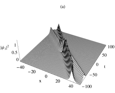
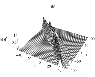
Figure 1: Intensity distribution in the coupled NLS equation for the parametric choice $a=1,b=1$,$\varepsilon_{1}^{(1)}=0.85i$,$\varepsilon_{1}^{(2)}=0.5$

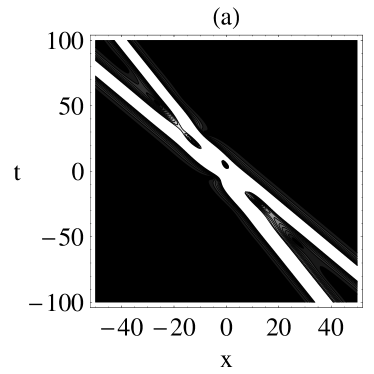
Figure 2: Trajectories of bright solitons in the two modes

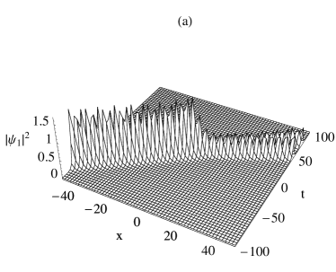
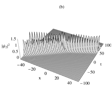
Figure 3: Realignment of intensity distribution for the parametric choice $a=1.5,b=1.5$, $\varepsilon_{1}^{(1)}=0.85i$, $\varepsilon_{1}^{(2)}=0.5$

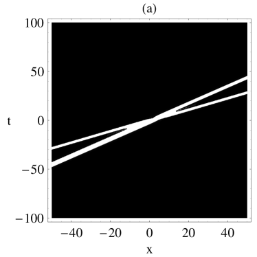
Figure 4: Rotation of the trajectories of bright solitons

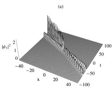
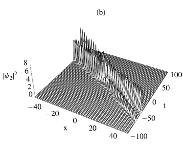
Figure 5: Further realignment of intensity distribution for the choice $a=2.5,b=2.5$,$\varepsilon_{1}^{(1)}=0.85i$,$\varepsilon_{1}^{(2)}=0.5$

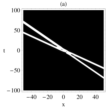
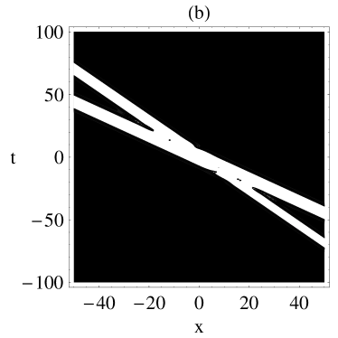
Figure 6: Enhanced rotation of the trajectories of bright solitons

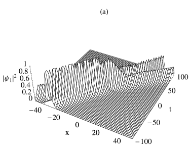
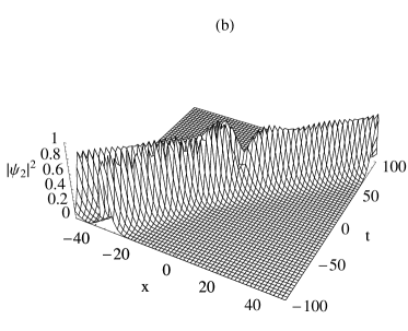
Figure 7: Collisional dynamics of bright solitons for the modified coupled NLS equation for $a=-b=0.9$, $\varepsilon_{1}^{(1)}=0.85i$, $\varepsilon_{1}^{(2)}=0.5$

Figure 8: Diagonally opposite trajectories of bright solitons in the modified coupled NLS equation

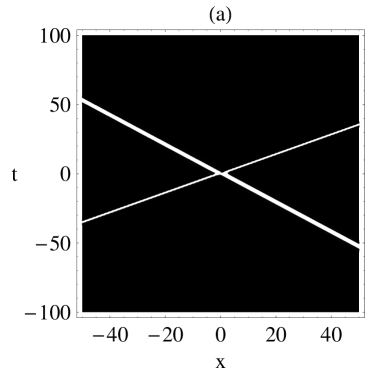
Figure 9: Enhancement of angular separation between the solitons by varying $\mu_{i},i=1,2$ for $\alpha_{10}=-0.1,\beta_{10}=-0.2,\alpha_{20}=0.15,\beta_{20}=0.3$ with the other parameters as in fig.3.

Figure 10: Further enhancement of angular separation between the solitons for $\alpha_{10}=-0.1,\beta_{10}=-0.25,\alpha_{20}=0.2,\beta_{20}=0.3$ with the other parameters as in fig.3.

III Results and Disscussion

Fig.1 shows the intensity distribution in the coupled NLS equation while the contour plot displayed in fig.2 shows their trajectories. When one changes the strengths of SPM and XPM, one observes a rotation of the trajectory of bright solitons besides the realignment of intensity distribution between the two modes as shown in fig.3. The contour plot shown in fig.4. confirms this observation. The angle of rotation of the trajectories can be further changed by varying the parameters a and b as shown in fig.5. and the corresponding contour plot is displayed in fig.6. Comparing the density profiles shown in fig (1) with figs (3) and (5), one understands that in addition to the rotation of trajectories of bright solitons, one also witnesses a realignment of intensity distribution between the modes $\psi_{1}$ and $\psi_{2}$. The rotation of the trajectories of bright solitons arises due to the extra energy that is being pumped into the dynamical system by varying the SPM and XPM parameters. This excess energy not only contributes to the rotation, but also to the realignment of intensity distribution.

It should be mentioned that the rotation of the trajectory of bright solitons is witnessed in the modified coupled NLS equation itself. For the intensity profile of the modified coupled NLS equation shown in fig.7., one observes shape changing collisional dynamics of bright solitons similar to coupled NLS equation. In addition, the trajectory of bright solitons is diagonally opposite (shown in fig.8) to that of what one observes in the coupled NLS equation (fig.2). The angular separation between the bright solitons can also be changed desirably by manipulating the complex hidden spectral parameter $\mu$ as shown in figs 9 and 10. It is worth noting that the variation of angular separation of bright solitons occurs in the coupled NLS equation itself, a fact which has not yet been noticed in the earlier studies.

From the above, one understands that the variation of SPM or XPM parameters injects extra energy into the dynamical system which not only results in the rotation of the trajectories of the bright solitons, but also in the realignment of their intensity distribution.

IV Conclusion

In summary, the collisional dynamics of bright solitons in the coupled NLS equation shows that apart from the intensity redistribution, one witnesses the rotation of the trajectories of bright solitons and realignment of intensity distribution between the two modes by varying the self phase modulation or cross phase modulation parameters. In addition, the angular separation between the bright solitons can also changed suitably. We believe that these results may stimulate a lot of experiments in nonlinear optics, Bose-Einstein condensates, left handed (LH) and right handed (RH) meta materials.

Acknowledgements Authors thank the referee for his invaluable suggestions. Authors would like to express their gratitude to Prof.M.Lakshmanan for his suggestions. PSV wishes to thank UGC and DAE-NBHM for the financial support. RR wishes to acknowledge the financial assistance received from DAE-NBHM (Ref.No:2/ 48(1)/ 2010 / NBHM /-R and D II/ 4524 dated May.11.2010), UGC (Ref.No:F.No 40-420/2011(SR) dated 4.July.2011) and DST (Ref.No:SR/S2/HEP-26/2012). KP acknowledges DST and CSIR, Government of India, for the financial support through major projects.

References

• (1) A.Hasegawa, F.Tappert, Applied. Phys. Lett. 23, 142 (1973); A.Hasegawa, F.Tappert, Applied. Phys. Lett. 23, 171 (1973).
• (2) L.F.Mollenauer, R.H.Stolen, J.P.Gordon, Phys.Rev.Lett. 45, 1095 (1980).
• (3) G.P.Agarwal, Nonlinear Fibre Optics, 5th edition (Academic Press, 2012).
• (4) N.E.Zakharov, E.I.Schulman, Physica D. 4, 270 (1982); R.Sahadevan, K. M. Tamizhmani and M. Lakshmanan, J. Phys. A. 19, 1783 (1986).
• (5) N.Akmediev, A.Ankiewicz, Solitons: Nonlinear Pulses and Beams, (Chapmen Hall, London, 1997); C R Menyuk, IEEE J. Quan. Elec. 23, 174 (1987); M. Wadati, T.Iizuka and M Hisakado, J. Phys. Soc. Japan.61, 2241 (1992); K. Porsezian and K. Nakkeeran, Pure and Applied Optics. 6, L7 (1997); M. Hisakado, T. Iizuka and M Wadati, J. Phys. Soc. Japan. 63, 2887 (1994).
• (6) S.V.Manakov, Sov.Phys.JETP. 38, 248 (1974).
• (7) D.J.Kaup, B.A.Malomed, Phys.Rev.A. 48, 599 (1993); F.Kh.Abdullaev , E.N.Tsoy, Physica D. 161, 67 (2002).
• (8) R.Radhakrishnan, M.Lakshmanan and J.Hietarinta, Phys.Rev.E. 56, 2213 (1997); R Radhakrishnan and M Lakshmanan, J. Phys. A. 28, 2683 (1995); M Hisakado and M Wadati, J. Phys. Soc. Japan. 64, 408 (1995);R Radhakrishnan and M Lakshmanan, Phys. Rev. E. 60, 2317 (1999).
• (9) V.G.Makhankov, N.V. Makhaldiani and O.K.Pashaev, Phys.Lett.A. 81, 161 (1981); T.Kanna, E.N.Tsoy and N.Akhmediev, Phys.Lett.A. 330, 224 (2004).
• (10) E.N.TSoy and N.Akhmediev, Optics Communication. 266,606 (2006).
• (11) Mohammed F. Saleh and Fabio Biancalana, Phys. Rev.A.87, 043807 (2013).
• (12) David Feijoo, Angel Paredes and Humberto Michinel, Phys. Rev.A. 87, 063619 (2013).
• (13) Bettina Gertjerenken, Thomas P. Billam, L. Khaykovich and Christoph Weiss, Phys.Rev.A. 86, 033608 (2012)
• (14) K. Nakkeeran, K. Porsezian, P. Shanmugha Sundaram, and A. Mahalingam, Phys. Rev. Lett. 80, 147 (1998).
• (15) R. H. Enns and S. S. Rangnekar, IEEE J. Quant. Elect. QE. 23, 1843 (1987); G.Cancellieri, F.Chiaraluce, E.Gambi and P.Pierleoni, J.Opt.Soc.Am.B. 12, 1300 (1995).
• (16) L.-L. Chau, J.C. Shaw and H.C. Yen, J. Math. Phys. 32,1737 (1991).