Direct Numerical Simulations of Reflection-Driven, Reduced MHD Turbulence from the Sun to the Alfvén Critical Point

Abstract

We present direct numerical simulations of inhomogeneous reduced magnetohydrodynamic (RMHD) turbulence between the Sun and the Alfvén critical point. These are the first such simulations that take into account the solar-wind outflow velocity and the radial inhomogeneity of the background solar wind without approximating the nonlinear terms in the governing equations. Our simulation domain is a narrow magnetic flux tube with a square cross section centered on a radial magnetic field line. We impose periodic boundary conditions in the plane perpendicular to the background magnetic field $\mathbf{B}_{0}$. RMHD turbulence is driven by outward-propagating Alfvén waves ($z^{+}$ fluctuations) launched from the Sun, which undergo partial non-WKB reflection to produce sunward-propagating Alfvén waves ($z^{-}$ fluctuations). Nonlinear interactions between $z^{+}$ and $z^{-}$ then cause fluctuation energy to cascade from large scales to small scales and dissipate. We present ten simulations with different values of the correlation time $\tau_{\rm c\,\sun}^{+}$ and perpendicular correlation length $L_{\perp\sun}$ of outward-propagating Alfvén waves (AWs) at the coronal base. We find that between 15% and 33% of the $z^{+}$ energy launched into the corona dissipates between the coronal base and Alfvén critical point, which is at $r_{\rm A}=11.1R_{\sun}$ in our model solar wind. Between 33% and 40% of this input energy goes into work on the solar-wind outflow, and between 22% and 36% escapes as $z^{+}$ fluctuations through the simulation boundary at $r=r_{\rm A}$. Except in the immediate vicinity of $r=R_{\sun}$, the $z^{\pm}$ power spectra scale like $k_{\perp}^{-\alpha^{\pm}}$, where $k_{\perp}$ is the wavenumber in the plane perpendicular to $\mathbf{B}_{0}$. In our simulation with the smallest value of $\tau_{\rm c\,\sun}^{+}$ ($\sim 2\mbox{ min}$) and largest value of $L_{\perp\sun}$ ($2\times 10^{4}\mbox{ km}$), we find that $\alpha^{+}$ decreases approximately linearly with increasing $\ln(r)$, reaching a value of 1.3 at $r=11.1R_{\sun}$. Our simulations with larger values of $\tau_{\rm c\,\sun}^{+}$ exhibit alignment between the contours of constant $\phi^{+}$, $\phi^{-}$, $\Omega_{0}^{+}$, and $\Omega_{0}^{-}$, where $\phi^{\pm}$ are the Elsässer potentials and $\Omega_{0}^{\pm}$ are the outer-scale parallel Elsässer vorticities. This alignment reduces the efficiency of nonlinear interactions at $r\gtrsim 2R_{\sun}$ to a degree that increases with increasing $\tau_{\rm c\,\sun}^{+}$.

I. Introduction

The solar wind is pervaded by turbulent fluctuations in the velocity, density, magnetic field, and electric field (Coleman, 1968; Belcher and Davis, 1971; Coles and Harmon, 1989; Bale et al., 2005; Wan et al., 2012). These fluctuations are only weakly compressive, in the sense that the fractional density fluctuations $\delta n/n$ are much less than $|\delta\mathbf{B}|/B$, where $\delta\mathbf{B}$ is the fluctuating magnetic field and $\mathbf{B}$ is the local magnetic field $\mathbf{B}$ (Tu and Marsch, 1995). Within the inertial range, $|\delta\mathbf{B}|\ll B$, $\delta\mathbf{B}$ is nearly perpendicular to $\mathbf{B}$, and $\delta\mathbf{B}$ varies more rapidly in the directions perpendicular to $\mathbf{B}$ than in the direction along $\mathbf{B}$ (Matthaeus et al., 1990; Tu and Marsch, 1995; Sahraoui et al., 2009; Chen et al., 2012). Together, these properties imply that most of the fluctuation energy in the inertial range can be described within the framework of reduced magnetohydrodynamics (RMHD) (Kadomtsev and Pogutse, 1974; Strauss, 1976; Zank and Matthaeus, 1992; Schekochihin et al., 2009). In this paper, we focus on the RMHD-like component of solar-wind turbulence, acknowledging that other types of fluctuations may also be present. Because Alfvén waves (AWs) are the linear wave mode of RMHD, we use the terms AWs, AW fluctuations and RMHD fluctuations interchangeably. For the same reason, we use the phrases AW turbulence and RMHD turbulence interchangeably.

Most of the AW fluctuations measured near Earth propagate away from the Sun in the solar-wind frame (Roberts et al., 1987), which suggests that AWs are launched into the solar wind from the Sun, consistent with observations of AW-like phenomena in the solar atmosphere (De Pontieu et al., 2007; Tomczyk et al., 2007). Parker (1965) suggested that the solar wind is largely heated and powered by AWs launched by the Sun. Because linear damping of AWs is extremely weak at large wavelengths (Barnes, 1966), a turbulent cascade of AW energy from large scales to small scales is needed if the AWs generated by the Sun are to heat the solar wind efficiently. On the other hand, a turbulent AW energy cascade requires nonlinear interactions between counter-propagating AWs (Iroshnikov, 1963; Kraichnan, 1965), and the Sun launches only outward-propagating AWs. In order for AWs to heat coronal holes and the solar wind, some source of inward-propagating AWs is thus needed.

Figure 1.— Radial profiles of $B_{0}$, $n$, $U$, and $v_{\rm A}$ used in our simulations.

One such source is the non-WKB reflection of AWs due to radial variations in the Alfvén speed $v_{\rm A}$ (Heinemann and Olbert, 1980; Velli, 1993; Hollweg and Isenberg, 2007). Photospheric motions generate AWs with periods $P$ of minutes to hours, corresponding to parallel wavelengths (measured in the direction of the background magnetic field $\mathbf{B}_{0}$) of $\sim Pv_{\rm A}$, which is $\gtrsim 1R_{\sun}$ in coronal holes (Cranmer and van Ballegooijen, 2005). These parallel wavelengths are comparable to the gradient lengthscales of the mass density $\rho$ and magnetic field $\mathbf{B}$ in coronal holes and the near-Sun solar wind, which causes outward-propagating AWs to undergo non-WKB reflection.

Recent work on reflection-driven RMHD turbulence falls into two categories. The first category consists of studies that employ simplified models of the nonlinear terms in the governing equations (Velli et al., 1989; Dmitruk et al., 2002; Cranmer and van Ballegooijen, 2005; Verdini and Velli, 2007; Chandran and Hollweg, 2009). The most sophisticated of these are the works of Verdini et al. (2009) and Verdini et al. (2012), who simulated reflection-driven RMHD turbulence from $r=1R_{\sun}$ out to $r\sim 20R_{\sun}$ using a shell model to approximate the nonlinear terms. The second category consists of direct numerical simulations of reflection-driven RMHD turbulence that retain the full nonlinear terms in the equations of inhomogeneous RMHD. As far as we are aware, there are only two previous studies in this category. Dmitruk and Matthaeus (2003) carried out simulations extending from the coronal base to a heliocentric distance $r$ of $2R_{\sun}$, neglecting the solar-wind outflow velocity. Van Ballegooijen et al. (2011) also neglected the solar-wind outflow velocity and carried out numerical simulations extending from the photosphere, through the chromosphere, and into the corona, focusing on closed coronal loops.

In this work, we present the first direct numerical simulations of inhomogeneous RMHD turbulence in coronal holes and the near-Sun solar wind that incorporate solar-wind outflow and wave reflection without approximating the nonlinear terms in the governing equations. Our simulations extend from the coronal base out to the Alfvén critical point, the point at which the solar-wind outflow speed equals the Alfvén speed, which is at $r=11.1R_{\sun}$ in our model solar wind. We describe our mathematical model in Section II and our numerical method in Section III. In Section IV, we analyze results from ten different numerical simulations. In Section V we discuss the inertial-range power spectra in the simulations, and the possible connection to the $\sim k^{-1}$ magnetic-field spectrum observed at small wavenumber $k$ in the interplanetary medium. In Section VI we describe an alignment effect that reduces the efficiency of nonlinear interactions in several of our simulations, and in Section VII we summarize our results and conclusions.

II. Open-Field RMHD model

We consider RMHD turbulence in a narrow magnetic flux tube centered on a radial magnetic field line extending outwards from the Sun. We define $x$ and $y$ to be Cartesian coordinates in the plane perpendicular to this central radial magnetic field line. The essence of our “narrow-flux-tube approximation” is the assumption that

$$\sqrt{x^{2}+y^{2}}\ll r.$$ (1)

That is, we restrict our analysis to the vicinity of the central radial field line. The equations that we present in this section can be viewed as the leading-order terms in an expansion in powers of $\theta_{\rm max}$, where $\theta_{\rm max}$ is an upper bound on the spherical polar angle $\theta$ in a spherical coordinate system in which $\theta=0$ corresponds to the central radial magnetic field line.

We take the mass density $\rho$, background magnetic field strength $B_{0}$, and solar-wind (proton) outflow velocity to be fixed functions of the distance $s$ measured along the magnetic field. Because of Equation (1), $s$ is approximately equal to the heliocentric distance $r$, and we can write

$$\rho=\rho(r),\quad\mathbf{U} = U(r)\mathbf{\hat{b}},\quad\mathbf{B}_{0}=B_{0}(r)\mathbf{\hat{b}},$$ (2)

where $\mathbf{\hat{b}}$ is the unit vector of the background magnetic field. The middle equality in Equation (2) expresses our assumption that $\mathbf{U}$ is parallel to $\mathbf{B}_{0}$. Since the flux tube is narrow, $\mathbf{\hat{b}}$ is approximately radial, and also approximately parallel to the magnetic field line at $x=y=0$. We adopt the same solar-wind profile as Chandran and Hollweg (2009), setting $\rho=m_{\rm p}n$ and

$$n(r)=\left(\frac{3.23\times 10^{8}}{\tilde{r}\,^{15.6}}+\frac{2.51\times 10^{6}}{\tilde{r}\,^{3.76}}+\frac{1.85\times 10^{5}}{\tilde{r}\,^{2}}\right)\mbox{ cm}^{-3},$$ (3)

where $\tilde{r}=r/R_{\sun}$, $m_{\rm p}$ is the proton mass, and $n$ is the proton number density. The first two terms on the right-hand side of Equation (3) are from Feldman et al. (1997), and the $r^{-2}$ term has been added so that $n$ extrapolates to the value $4\mbox{ cm}^{-3}$ at $r=1\mbox{ AU}$. The background field strength is given by

$$B_{0}=\left[\frac{1.5(f_{\rm max}-1)}{\tilde{r}\,^{6}}+\frac{1.5}{\tilde{r}\,^{2}}\right]\mbox{ Gauss},$$ (4)

where $f_{\rm max}$ is the usual super-radial expansion factor, which we set equal to 5. The solar-wind speed then follows from flux conservation,

$$U=9.25\times 10^{12}\;\frac{B_{\rm G}}{\tilde{n}}\;\mbox{cm}\;\mbox{s}^{-1},$$ (5)

where $B_{\rm G}$ is $B_{0}$ in Gauss and $\tilde{n}$ is $n$ in units of $\mbox{cm}^{-3}$. The normalization constant in Equation (5) has been chosen so that $U=750\;\mbox{km}\;\mbox{s}^{-1}$ at 1 AU. The Alfvén critical point in this model is at $r_{a}=11.1R_{\sun}$, and the maximum of $v_{\rm A}$ is at $r_{m}=1.60R_{\sun}$. The magnetic field strength, density, solar-wind speed, and Alfvén speed are plotted in Figure 1.

We consider non-compressive fluctuations in the velocity $\delta\mathbf{v}$ and magnetic field $\delta\mathbf{B}$ within this narrow flux tube. We assume that $\delta\mathbf{v}\cdot\mathbf{\hat{b}}=0$, $\delta\mathbf{B}\cdot\mathbf{\hat{b}}=0$ and that the fluctuations vary on lengthscales in the directions perpendicular to $\mathbf{B}_{0}$ that are much smaller than $r$ and much smaller than the lengthscales on which the fluctuations vary in the direction parallel to $\mathbf{B}_{0}$. We further assume that $\delta B\ll B_{0}$ and that the characteristic lengthscales and timescales of the fluctuations are $\gg\rho_{\rm p}$ and $\Omega_{\rm p}^{-1}$, where $\rho_{\rm p}$ and $\Omega_{\rm p}$ are the proton gyroradius and cyclotron frequency. Given these assumptions, the fluctuations are well described by the equations of inhomogeneous RMHD (Heinemann and Olbert, 1980; Velli et al., 1989), which can be written in the form

$$\frac{\partial\mathbf{z}^{\pm}}{\partial t}+\left(U\pm v_{\rm A}\right)\frac{\partial\mathbf{z}^{\pm}}{\partial r}+\left(U\mp v_{\rm A}\right)\left(\frac{\mathbf{z}^{\pm}}{4H_{\rho}}-\frac{\mathbf{z}^{\mp}}{2H_{\rm A}}\right)$$

$$=-\mathbf{z}^{\mp}\cdot\mathbf{\nabla}_{\perp}\mathbf{z}^{\pm}-\frac{\nabla_{\perp}P}{\rho}-\nu_{p}(-\nabla_{\perp}^{2})^{p}\mathbf{z}^{\pm},$$ (6)

where

$$\mathbf{z}^{\pm} = \delta\mathbf{v}\mp\frac{\delta\mathbf{B}}{\sqrt{4\pi\rho}},$$ (7)

$$\nabla_{\perp} = \mathbf{e}_{x}\frac{\partial}{\partial x}+\mathbf{e}_{y}\frac{\partial}{\partial y},$$ (8)

$$H_{\rho}^{-1} = -\rho^{-1}d\rho/dr,$$ (9)

$$H_{B}^{-1} = -B_{0}^{-1}dB_{0}/dr,$$ (10)

$$H_{\rm A}^{-1} = v_{\rm A}^{-1}dv_{\rm A}/dr,$$ (11)

$p$ is an integer $\geq 1$, and $\nu_{p}(r)$ is a positive definite hyperviscosity coefficient. The hyperviscosity term in Equation (6), which will be discussed in more detail in Section III, has been added to act as a sink of energy in the system at small (perpendicular) lengthscales to ensure numerical stability.

Equation (6) contains a key piece of physics that is not present in the homogeneous RMHD model, namely the linear coupling between $\mathbf{z}^{+}$ and $\mathbf{z}^{-}$ fluctuations through the $H_{\rm A}^{-1}$ term. This linear coupling is responsible for the non-WKB reflection of AWs. As $H_{\rho}$ and $H_{\rm A}$ are increased to infinity, Equation (6) reduces to the usual equations of homogeneous RMHD.

The Elsässer potentials $\phi^{\pm}$ are related to $\mathbf{z}^{\pm}$ through the equation

$$\mathbf{z}^{\pm}=\mathbf{\hat{b}}\times\nabla\phi^{\pm},$$ (12)

and the field-aligned Elsässer vorticity is given by

$$\Omega^{\pm}=\mathbf{\hat{b}}\cdot\nabla\times\mathbf{z}^{\pm}=\nabla_{\perp}^{2}\phi^{\pm}.$$ (13)

By taking the curl of (6) and taking the dot product of the resulting equation with $\mathbf{\hat{b}}$, we obtain

$$\frac{\partial\Omega^{\pm}}{\partial t} + \left(U\pm v_{\rm A}\right)\left(\frac{\partial\Omega^{\pm}}{\partial s}-\frac{\Omega^{\pm}}{2H_{B}}\right)$$

$$+ \left(U\mp v_{\rm A}\right)\left(\frac{1}{4H_{\rho}}\Omega^{\pm}-\frac{1}{2H_{\rm A}}\Omega^{\mp}\right)$$

$$= -\mathbf{\hat{b}}\cdot\left[\nabla\times(\mathbf{z}^{\mp}\cdot\mathbf{\nabla}\mathbf{z}^{\pm})\right]-\nu_{p}(-\nabla_{\perp}^{2})^{p}\Omega^{\pm}.$$

Equation (LABEL:eq:vorticity) extends the RMHD model for coronal loops of van Ballegooijen et al. (2011) to include a background solar wind flow $U$.

III. Numerical Method and the IRMHD Code

We solve Equation (LABEL:eq:vorticity) in a simulation domain that consists of a narrow magnetic flux tube with a square cross section extending from a heliocentric distance of $r_{\rm min}=1R_{\sun}$ (the coronal base) out to the Alfvén critical point $r_{\rm max}=r_{\rm A}$ ($11.1R_{\sun}$ in our model) at which $U=v_{\rm A}$, as illustrated in Figure 2. We define $L_{\perp}(r)$ to be the dimension of the simulation domain perpendicular to $\mathbf{B}_{0}$ at heliocentric distance $r$, and $L_{\perp\sun}$ to be the value of $L_{\perp}(r)$ at $r=r_{\rm min}$. Because the magnetic flux through the flux-tube cross section is independent of $r$,

$$L_{\perp}(r)=L_{\perp\sun}\sqrt{\frac{B_{0}(r_{\rm min})}{B_{0}(r)}}.$$ (15)

Given Equation (4), $L_{\perp}$ expands by a factor of 24.8 between $r_{\rm min}$ and $r_{\rm max}$. In half of our simulations, we set $L_{\perp\sun}=10^{4}$ km, and in the other half we set $L_{\perp\sun}=2\times 10^{4}$ km. At all $r$, $L_{\perp}/r<0.032$ when $L_{\perp\sun}=10^{4}\mbox{ km}$, and $L_{\perp}/r<0.064$ when $L_{\perp\sun}=2\times 10^{4}\mbox{ km}$, consistent with Equation (1).

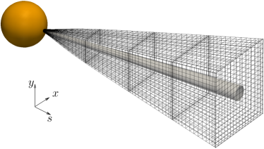
Figure 2.— Numerical domain and coordinates employed by our IRMHD turbulence code. (See text for details.)

Because $L_{\perp}\ll r$, we can neglect the curvature of surfaces perpendicular to $\mathbf{B}_{0}$ when solving Equation (LABEL:eq:vorticity) and treat these surfaces as planes. At each $r$, we employ $N_{\perp}$ uniformly spaced grid points in each of the $x$ and $y$ directions, where $N_{\perp}$ is independent of $r$. Since $L_{\perp}(r)$ increases with $r$, the grid spacing in $x$ and $y$ increases with $r$. We take the $\mathbf{z}^{\pm}$ fluctuations to satisfy periodic boundary conditions in the $x-y$ plane. However, as we will discuss further below, radial inhomogeneity prevents us from using periodic boundary conditions in the $r$ direction.

Equation (LABEL:eq:vorticity) represents a system of two coupled partial differential equations (PDEs), one for $\Omega^{+}(\mathbf{x}_{\perp},r,t)$ and one for $\Omega^{-}(\mathbf{x}_{\perp},r,t)$, where $\mathbf{x}_{\perp}=x\mathbf{e}_{x}+y\mathbf{e}_{y}$ is the position vector in the $x-y$ plane. The code that we have developed for this investigation, called the Inhomogeneous RMHD Code, or IRMHD Code, solves this system of PDEs using a spectral element method (SEM) based on a Chebyshev-Fourier basis (Canuto et al., 1988). The essence of the SEM method is to perform a decomposition of the domain along the radial direction into $M$ subdomains $\mathcal{D}_{n}$, where $n=1,2,\ldots,M$. The Elsässer vorticities (and, analogously, $\mathbf{z}^{\pm}$ and $\phi^{\pm}$) are approximated by a truncated Chebyshev-Fourier expansion in each subdomain,

$$\left.\Omega^{\pm}(\mathbf{x}_{\perp},r,t)\right|_{\mathcal{D}_{n}}=\sum_{\alpha\tilde{k}_{x}\tilde{k}_{y}}\Omega^{\pm}_{\alpha\tilde{k}_{x}\tilde{k}_{y},n}(t)T_{\alpha}(\xi_{n})\exp(i\mathbf{k_{\perp}}\cdot\mathbf{x}_{\perp}),$$ (16)

where

$$\mathbf{k}_{\perp}=\frac{2\pi\tilde{\mathbf{k}}_{\perp}}{L_{\perp}(r)}$$ (17)

is the perpendicular wavevector, $\tilde{\mathbf{k}}_{\perp}=\tilde{k}_{x}\mathbf{e}_{x}+\tilde{k}_{y}\mathbf{e}_{y}$, and $T_{\alpha}(\xi_{n})=\cos(\alpha\cos^{-1}\xi_{n})$ is the Chebyshev polynomial of order $\alpha$. The quantity $\xi_{n}=2(r-r_{n})/\Delta r_{n}$ is the normalized radial coordinate in sub-domain $\mathcal{D}_{n}$, where $r_{n}$ is the radial midpoint of the $n^{\rm th}$ subdomain, and $\Delta r_{n}$ is the length of the $n^{\rm th}$ subdomain in the $r$ direction. Within the $n^{\rm th}$ subdomain, we discretize the radial interval using the Gauss-Lobatto grid, $\xi_{n,j}=\cos(\pi j/N_{d})$, where $N_{d}$ is the number of radial grid points per subdomain. This choice of grid enables us to carry out the Chebyshev transform using a fast cosine transform and to retain the exponential accuracy characteristic of spectral methods. The quantities $\tilde{k}_{x}$, $\tilde{k}_{y}$, and $\alpha$ take on integer values only, with $-N_{\perp}/2+1\leq\tilde{k}_{x}\leq N_{\perp}/2$, $-N_{\perp}/2+1\leq\tilde{k}_{y}\leq N_{\perp}/2$, and $0\leq\alpha<N_{d}$. This Chebyshev-Fourier expansion results in a system of ordinary differential equations (ODEs) for the Chebyshev-Fourier coefficients $\Omega^{\pm}_{\alpha\tilde{k}_{x}\tilde{k}_{y},n}(t)$ in each subdomain. These equations are coupled through boundary conditions (continuity of $\mathbf{z}^{\pm}$) at the interface surfaces.

As discussed in Section II, the hyperviscosity term in Equation (6) dissipates the fluctuations before they can cascade to the grid-scale. We set

$$\nu_{p}(r)=\tilde{\nu}_{p}\left[\frac{L_{\perp}(r)}{2\pi}\right]^{2p}$$ (18)

with $p=4$ and $\tilde{\nu}=5\times 10^{-5}z^{+}_{\rm{rms}\sun}/L_{\sun}$, where $z^{+}_{\rm{rms}\sun}$ is the imposed amplitude of $z^{+}$ fluctuations at $r=R_{\sun}$ (see section IV). The Chebyshev-Fourier coefficients of the hyperviscosity term in Equation (LABEL:eq:vorticity) within the $n^{\rm th}$ radial subdomain are then simply $-\tilde{\nu}_{p}\tilde{k}_{\perp}^{2p}\Omega^{\pm}_{\alpha\tilde{k}_{x}\tilde{k}_{y},n}$. We advance the solution to Equation (LABEL:eq:vorticity) forward in time using a third-order Runge-Kutta method and employ an integrating factor to handle the hyperviscosity term. With this approach, the time step is not limited by the hyperviscous timescale, and is instead constrained solely by the accuracy and stability requirements of the non-dissipative terms. For initial conditions, we set

$$\left.\Omega^{\pm}(\mathbf{x}_{\perp},r,t=0)\right|_{\mathcal{D}_{n}}=0$$ (19)

at all $\mathbf{x}_{\perp}$ and $r$.

The IRMHD code uses the Message Passing Interface (MPI) programming paradigm and possesses excellent scaling properties on massively parallel supercomputers due to the nature of the domain decomposition in the SEM algorithm. To parallelize the code, we assign each subdomain to a different set of processors, with the appropriate communications between domains to transfer boundary information, maintaining a low network overhead. The single-domain component of the IRMHD code is a fully de-aliased 3D Chebyshev-Fourier pseudo-spectral algorithm that performs spatial discretization on a grid with $N_{\perp}^{2}\times N_{d}$ grid points. This decomposition results is a global mesh of $N_{\perp}^{2}\times N_{r}$ grid points where $N_{r}=(N_{d}-1)M+1$ is total number of radial points from all the subdomains. For the simulations described in Section III, $N_{d}=17$ and $M=512$, which leads to $N_{r}=8193$, and $\Delta r_{n}$ is taken to be the same for each subdomain, which leads to $\Delta r_{n}\simeq 0.02R_{\sun}$. Within each subdomain, we parallelize the 2D fast Fourier transform in the $x-y$ plane. In low-resolution runs, we turn off this “intra-domain” parallelization, assigning one processor per subdomain. However, for the runs reported in this paper, 16 processors per subdomain were used, requiring a total of 8192 processors in a single simulation. We have verified the accuracy of the IRMHD code through extensive tests of linear wave propagation and reflection and nonlinear conservation of wave action.

III.1. Radial Boundary conditions

The equations describing the evolution of $\Omega^{+}$ and $\Omega^{-}$ are hyperbolic advection equations, where $\Omega^{+}$ is advected at radial velocity $U+v_{\rm A}$ and $\Omega^{-}$ is advected at radial velocity $U-v_{\rm A}$. The radial velocity of $\Omega^{-}$ is negative at $r<r_{\rm A}$, where $U<v_{\rm A}$, and positive at $r>r_{\rm A}$. Given that $U+v_{\rm A}>0$, one must specify one boundary condition on $\Omega^{+}$ at the lower boundary $r=R_{\sun}$ to solve the advection PDE for $\Omega^{+}$. This boundary condition determines the properties of the $\mathbf{z}^{+}$ fluctuations that are advected into the simulation domain at $r=R_{\sun}$ and contains all our assumptions about the properties of the Alfvén waves that are launched by the Sun, including their amplitudes, perpendicular wavelengths, and frequencies. It would be natural to expect that an additional boundary condition is required to solve the advection equation for $\Omega^{-}$ at the outer boundary of the simulation at $r=r_{\rm max}$ to determine the amplitudes of the inward waves that are injected towards the Sun from radii exceeding $r_{\rm max}$. However, an outer boundary condition on $\mathbf{z}^{-}$ is only necessary if $r_{\rm max}<r_{\rm A}$, in which case the radial velocity $U-v_{\rm A}$ of the $\mathbf{z}^{-}$ waves is negative at $r_{\rm max}$. In the simulations that we present in this work, we set $r_{\rm max}=r_{\rm A}$, and thus $\mathbf{z}^{-}$ waves do not flow into the simulation domain at $r=r_{\rm A}$. Mathematically, this means that no additional boundary condition needs to be (or in fact can be) imposed on $\mathbf{z}^{-}$ at the outer boundary. If instead we were to set $r_{\rm max}<r_{\rm A}$ and impose an extra outer boundary condition on $\mathbf{z}^{-}$, then this boundary condition would amount to an unphysical assumption that would modify the correct solution that arises when the Alfvén critical point is included in the domain.

At $r=r_{\rm min}$, we impose the random, time-dependent boundary condition $\mathbf{z}^{+}(\mathbf{x},r=r_{\rm min},t)=\mathbf{z}_{\rm b}^{+}(\mathbf{x}_{\perp},t)$, where

$$\mathbf{z}_{\rm b}^{+}(\mathbf{x}_{\perp},t)=\sum_{\tilde{k}_{x}\tilde{k}_{y}}i\,\mathbf{\hat{b}}\times\mathbf{k}_{\perp}\phi_{b\tilde{k}_{x}\tilde{k}_{y}}(t)\exp{\left(i\mathbf{k}_{\perp}\cdot\mathbf{x}_{\perp}\right)},$$ (20)

$$\phi_{b\tilde{k}_{x}\tilde{k}_{y}}=\left\{\begin{array}[]{cc}C\zeta_{\tilde{k}_{x}\tilde{k}_{y}}(t)&1\leq\tilde{k}_{\perp}\leq 3\\ &\\ 0&\hbox{otherwise}\end{array}\right..$$ (21)

We set $\zeta_{\tilde{k}_{x}\tilde{k}_{y}}(t_{j})=\tilde{k}_{\perp}^{-9/4}\exp{\left(i\psi_{j,\tilde{k}_{x}\tilde{k}_{y}}\right)}$, where $t_{\rm j}=j\tau_{\rm b}$, $j=-1,0,1,2,\dots$, and $\psi_{j,\tilde{k}_{x}\tilde{k}_{y}}$ are uniformly distributed random phases between $0$ and $2\pi$. At values of $t$ between consecutive $t_{\rm j}$, we determine $\zeta_{\tilde{k}_{x}\tilde{k}_{y}}(t)$ using the cubic-interpolation algorithm described by Keys (1981). We adjust the constants $C$ and $\tau_{\rm b}$ to control the rms value of $z^{+}$ at the inner boundary, denoted $z^{+}_{\rm rms\,\sun}$, and the correlation time $\tau_{\rm c\,\sun}^{+}$ of $z^{+}$ at $r=R_{\sun}$ (defined in Equation (27) below). As a rough rule of thumb, $\tau_{\rm c\,\sun}^{+}\simeq 0.5\tau_{\rm b}$. Because $z^{+}=0$ at all points inside the domain at $t\leq 0$, we choose the coefficients $\zeta_{\tilde{k}_{x}\tilde{k}_{y}}(t_{j})$ for $j=-1,0$ and $1$ in such a way that both $\mathbf{z}_{\rm b}^{+}(\mathbf{x}_{\perp},t=0)$ and $\partial_{t}\mathbf{z}_{\rm b}^{+}(\mathbf{x}_{\perp},t=0)$ vanish. This prevents the propagation of abrupt radial variations into the domain at early times.

Simulation	$L_{\perp\sun}$	$\tau^{+}_{\rm c\,\sun}$	$z^{+}_{\rm rms\,\sun}$	$\tau_{nl,\sun}^{+}$	$\tau_{nl,\sun}^{-}$	Run time
	($10^{3}$ km)	(min)	(km/s)	(min)	(min)	(h)
A1	10	19.7	42	3.01	0.66	16.3
A2	20	22.4	40	4.85	1.32	16.4
B1	10	9.9	42	2.78	0.66	11.8
B2	20	9.9	40	4.35	1.32	13.3
C1	10	6.0	42	2.59	0.66	11.5
C2	20	6.7	40	4.03	1.32	12.1
D1	10	3.3	41	2.33	0.66	11.6
D2	20	3.3	40	4.18	1.33	12.9
E1	10	2.0	41	2.40	0.67	33.4
E2	20	2.0	40	4.34	1.34	31.2

Table 1Simulation labels and parameter values. The quantity $L_{\perp\sun}$ is the width of the simulation-domain cross section at $r=R_{\sun}$, $\tau^{+}_{\rm c\,\sun}$ is the the correlation time of the $z^{+}$ AWs launched into the simulation domain at $r=R_{\sun}$, $\tau_{\rm nl,\sun}^{\pm}=(k_{\perp\sun}z^{\mp}_{\rm rms})^{-1}$ is the nonlinear timescale of $z^{\pm}$ fluctuation at $r=R_{\sun}$, and the run time is $t_{\rm f}-t_{\rm i}$, where $t_{\rm i}=0$ and $t_{\rm f}$ are the values of $t$ at the beginning and end of each simulation.

As mentioned previously, since we choose $r_{\rm max}\geq r_{\rm A}$ no additional boundary condition needs to be imposed for $\mathbf{z}^{-}$. The value of $z^{-}$ at the the Alfvén critical point, which we denote $z^{-}_{\rm A}$, satisfies the equation

$$\frac{\partial\mathbf{z}_{\rm A}^{-}}{\partial t}+2v_{\rm A}\left(\frac{1}{4H_{\rho}}\mathbf{z}_{\rm A}^{-}-\frac{1}{2H_{v_{\rm A}}}\mathbf{z}_{\rm A}^{+}\right)=-\left(\mathbf{z}_{\rm A}^{+}\cdot\nabla\right)\mathbf{z}_{\rm A}^{-},$$ (22)

where $\mathbf{z}_{\rm A}^{+}$ is the value of $\mathbf{z}^{+}$ at $r=r_{\rm A}$. At $t=0$, $z_{\rm A}^{-}=0$, from Equation (19). To determine $\mathbf{z}_{\rm A}^{-}$ at all subsequent times, we integrate Equation (22) forward in time, using the time-evolving numerical solution for $\mathbf{z}^{+}$ at $r=r_{\rm A}$. Note that the pressure and dissipation terms have been omitted for simplicity

Figure 3.— Time evolution of $E_{\rm tot}^{\pm}$ for the simulations in Table 1.

IV. Numerical Simulations

In this section, we report the results of ten numerical simulations carried out using the numerical method described in Section III. Each simulation uses $256^{2}\times 8193$ grid points. There are three adjustable physical parameters in the simulations: the rms amplitude and correlation time, $z^{+}_{\rm rms\,\sun}$ and  $\tau_{\rm c\,\sun}$, of the $z^{+}$ waves that are injected into the simulation domain at $r=R_{\sun}$ and the width $L_{\perp\sun}$ of the cross section of the simulation domain at $r=R_{\sun}$. The values of these parameters in each simulation are listed in Table 1. The values chosen for $\tau_{\rm c\sun}^{+}$ are motivated by observations of magnetic bright points and photospheric motions, which suggest that the dominant timescales of AWs launched into the Sun range from minutes to hours (Cranmer and van Ballegooijen, 2005; Verdini and Velli, 2007). Previous studies of AW launching by the Sun have considered values for the dominant AW correlation length perpendicular to $\mathbf{B}_{0}$ at $r=r_{\rm min}$ ranging from granular scales $\sim 10^{3}\mbox{ km}$ (Cranmer and van Ballegooijen, 2005; Hollweg et al., 2010) to scales $\sim 5\times 10^{3}\mbox{ km}$ comparable to the spacing of photospheric flux tubes (Chandran and Hollweg, 2009) to scales of $10^{4}\mbox{ km}-3\times 10^{4}\mbox{ km}$ corresponding to the diameters of supergranules (Dmitruk et al., 2002; Verdini and Velli, 2007; Verdini et al., 2012). In our simulations, this perpendicular correlation length is $\sim L_{\perp\sun}$, and we set $L_{\perp\sun}=10^{4}$ km or $L_{\perp\sun}=2\times 10^{4}\mbox{ km}$. For all of the simulations reported in this paper, we take $z^{+}_{\rm b,rms}=40\mbox{ km/s}$. This choice results in an rms velocity fluctuation at $r=r_{\rm min}$, denoted $\delta v_{\rm rms\sun}$, that satisfies

$$\delta v_{\rm rms\,\sun}\simeq 20\mbox{ km/s},$$ (23)

in agreement with Hinode measurements of the transverse motions of field-aligned structures in the low corona (De Pontieu et al., 2007).

Although the values we have used for $\tau_{\rm c\,\sun}$, $L_{\perp\sun}$, and $z^{+}_{\rm rms\sun}$ are plausible, there is considerable uncertainty in the values of these parameters in the solar atmosphere. For example, the moving spicules observed by De Pontieu et al. (2007) have proton densities $\gtrsim 10^{13}\mbox{ cm}^{-3}$ that are much larger than the value $n_{\rm p}\simeq 3\times 10^{8}\mbox{ cm}^{-3}$ that typifies coronal holes at $r\simeq 1R_{\sun}$ (Feldman et al., 1997). The mass loading of these spicules may slow their transverse motions relative to the motions of the surrounding lower-density regions. In addition, the Sun likely launches AWs with a broad spectrum of timescales and perpendicular correlation lengths, a point to which we return in Section V. A more comprehensive exploration of wave-launching scenarios would be useful, but is beyond the scope of this paper.

Figure 4.— Radial dependence of relevant timescales in the simulations: The reflection timescale $\tau_{r}$ (long-dash), $z^{+}$ autocorrelation time $\tau^{+}_{\rm c}$ (solid), $z^{-}$ autocorrelation time $\tau^{-}_{\rm c}$ (dash-dot), the nominal eddy turnover time $\tau^{+}_{\rm nl}$ (dash) and the nominal eddy turnover time $\tau^{-}_{\rm nl}$ (dash-triple-dot).

IV.1. Timescales

The $z^{+}$ AWs injected into the domain at $r=r_{\rm min}$ propagate away from the Sun and generate $z^{-}$ waves via non-WKB reflection. These $z^{-}$ waves undergo further reflections, producing more $z^{+}$ fluctuations, and also interact nonlinearly with the $z^{+}$ AWs, producing a turbulent cascade. In each of our simulations, we evolve the Elsässer fields until they reach an approximate statistical steady state, which occurs after approximately 4 hours of physical time in Simulations A1 through E1, and 5 hours of physical time in Simulations A2 through E2. This approach to steady state is illustrated in Figure 3, which shows the time evolution of the total $z^{\pm}$ energy

$$E_{\rm tot}^{\pm}=\frac{1}{4}\,\int d^{3}x\,\rho|\mathbf{z}^{\pm}|^{2},$$ (24)

where the volume integral is over the entire simulation domain.

An important timescale for these simulations is the $z^{+}$ Alfvén crossing time $\tau_{\rm A}$, which is the time it takes a $z^{+}$ fluctuation to travel from $r_{\rm min}$ to $r_{\rm max}$,

$$\tau_{\rm A}=\int_{r_{\rm min}}^{r_{\rm max}}\frac{dr}{U(r)+v_{\rm A}(r)}\simeq 1.3\mbox{ hours}.$$ (25)

We define the nominal nonlinear timescale for the large-scale $z^{\pm}$ fluctuations through the equation

$$\tau_{\rm nl}^{\pm}(r)=(k_{\perp\rm min}z^{\mp}_{\rm rms})^{-1},$$ (26)

where $k_{\perp\rm min}=2\pi/L_{\perp}(r)$ is the minimum perpendiucular wavenumber at radius $r$. This is the approximate timescale on which $z^{\pm}$ fluctuations at perpendicular scale $L_{\perp}$ are sheared by $z^{\mp}$ fluctuations at perpendicular scale $L_{\perp}$, where $z^{\mp}_{\rm rms}(r)$ is the rms value of $z^{\mp}$ at heliocentric distance $r$. We define the correlation time $\tau_{\rm c}^{\pm}$ of the (outer-scale) $z^{\pm}$ fluctuations at radius $r$ through the equation

$$C^{\pm}(r,\tau_{\rm c}^{\pm})=e^{-1},$$ (27)

where

$$C^{\pm}(r,\tau)=\frac{\langle\mathbf{z}^{\pm}(\mathbf{x}_{\perp},r,t)\cdot\mathbf{z}^{\pm}(\mathbf{x}_{\perp},r,t+\tau)\rangle}{\langle\mathbf{z}^{\pm}(\mathbf{x}_{\perp},r,t)\cdot\mathbf{z}^{\pm}(\mathbf{x}_{\perp},r,t)\rangle},$$ (28)

and $\langle\dots\rangle$ denotes an average over $x$, $y$, and $t$. We also define the reflection timescale

$$\tau_{\rm r}=\left(\frac{dv_{\rm A}}{dr}\right)^{-1}$$ (29)

that characterizes the $H_{\rm A}^{-1}$ term in Equation (6), which is the only linear term in Equation (6) that couples $\mathbf{z}^{+}$ with $\mathbf{z}^{-}$.

We plot the timescales $\tau_{\rm nl}^{\pm}$, $\tau_{\rm c}$, and $\tau_{\rm r}$ as functions of $r$ in Figure 4. In Simulations A1 through C1 and A2 through C2, $\tau_{\rm c\,\sun}^{+}$ exceeds $\tau_{\rm r}(R_{\sun})$, which causes reflection to be very efficient near $R_{\sun}$. The nonlinear timescale $\tau_{\rm nl}^{+}$ is significantly larger than $\tau_{\rm nl}^{-}$ at all $r$ and in all simulations because $z^{-}_{\rm rms}<z^{+}_{\rm rms}$. In Simulations A1, A2, B1, and B2, $\tau_{\rm c}^{+}$ is significantly larger than $\tau_{\rm nl}^{+}$ at small $r$ due to the large coherence time of the the waves that are launched at $r=R_{\sun}$.

Figure 5.— Top four panels show the radial dependence of the rms amplitudes of $\mathbf{z}^{\pm}$, $\delta\mathbf{B}$, and $\delta\mathbf{v}$. The bottom two panels show the radial profiles of the fractional cross-helicity $\sigma_{\rm c}$ and the fractional residual energy $\sigma_{\rm r}$.

The correlation times $\tau_{\rm c}^{+}$ and $\tau_{\rm c}^{-}$ are comparable to each other at all $r$ exceeding $\sim 2R_{\sun}$ in Simulations A1 through D1 and A2 through D2. In these simulations, $\tau_{\rm nl}^{-}<\tau_{\rm c}^{+}$, and the outer-scale $z^{+}$ fluctuations imprint their correlation time onto the outer-scale $z^{-}$ fluctuations through nonlinear interactions. In contrast, in Simulations E1 and E2, $\tau_{\rm nl}^{-}>\tau_{\rm c}^{+}$ at large $r$, and nonlinear interactions are too weak for the outer-scale $z^{+}$ fluctuations to transfer their correlation timescale to the outer-scale $z^{-}$ fluctuations. In these simulations at large $r$, $\tau_{\rm c}^{-}>\tau_{\rm c}^{+}$, presumably because radial inhomogeneities preferentially reflect the lower-frequency component of $z^{+}$.

We note that after the simulations have reached an approximate statistical steady state, we continue to evolve the fields for an additional time of at least $\simeq 7\mbox{ hours}$. This additional time is $\gtrsim 5\tau_{\rm A}$, $\gtrsim 18\tau^{+}_{\rm c\sun}$ and $\gtrsim 86\tau_{nl,\sun}^{+}$ in all simulations. When we take time averages, we restrict the time averaging to this approximate-steady-state period.

IV.2. Radial Profiles

In Figure 5, we plot the radial profiles of $z^{\pm}_{\rm rms}$, the rms values of $\delta\mathbf{v}$ and $\delta\mathbf{B}$ (denoted $\delta v_{\rm rms}$ and $\delta B_{\rm rms}$), the fractional cross helicity

$$\sigma_{\rm c}(r)=\frac{[z^{+}_{\rm rms}(r)]^{2}-[z^{-}_{\rm rms}(r)]^{2}}{[z^{+}_{\rm rms}(r)]^{2}+[z^{-}_{\rm rms}(r)]^{2}},$$ (30)

and the fractional residual energy

$$\sigma_{\rm r}(r)=\frac{4\pi\rho[\delta v_{\rm rms}(r)]^{2}-[\delta B_{\rm rms}(r)]^{2}}{4\pi\rho[\delta v_{\rm rms}(r)]^{2}+[\delta B_{\rm rms}(r)]^{2}}.$$ (31)

The fractional cross helicity is highest for the runs with the smallest values of $\tau_{\rm c\,\sun}^{+}$, because shorter correlation times at the coronal base translate to higher wave frequencies throughout the domain, which reduces the efficiency of non-WKB wave reflection. The maximum value of $\delta B/B_{0}$ occurs in Simulation A1 at $r=r_{\rm max}$, where $\delta B/B_{0}=0.37$. The assumption that $\delta B\ll B_{0}$ underlying Equation (6) is thus at least marginally satisfied in all of the simulations. The sign of the residual energy depends upon $r$. At $r<1.6R_{\sun}$, $dv_{\rm A}/dr>0$ and wave reflections act to create positive residual energy. At $r>1.6R_{\sun}$, $dv_{\rm A}/dr<0$ and wave reflections are a source of negative residual energy. Because the $z^{-}$ waves propagate towards smaller $r$ after being produced by reflections, the transition from positive to negative $\sigma_{\rm r}$ occurs at $r<1.6R_{\sun}$.

IV.3. Power Spectra

Once the fluctuations reach a statistical steady state, the average $z^{\pm}$ energy density per unit mass,

$$u^{\pm}(r)=\frac{1}{4}\left\langle\mathbf{z}^{\pm}(\mathbf{x}_{\perp},r,t)\cdot\mathbf{z}^{\pm}(\mathbf{x}_{\perp},r,t)\right\rangle,$$ (32)

is a function of $r$ alone. As in section IV.1, the average is taken over $x,y$ and $t$. After expanding $\mathbf{z}^{\pm}$ in the Fourier series

$$\mathbf{z}^{\pm}(\mathbf{x}_{\perp},r,t)=\sum_{\tilde{k}_{x}}\;\sum_{\tilde{k}_{y}}\tilde{\mathbf{z}}^{\pm}_{\tilde{k}_{x}\tilde{k}_{y}}(r,t)e^{i\mathbf{k}_{\perp}\cdot\mathbf{x}_{\perp}},$$ (33)

where $\tilde{k}_{x}$ and $\tilde{k}_{y}$ (defined in Equation (17)) take on integer values only, we can rewrite Equation (32) as

$$u^{\pm}(r) = \sum_{\tilde{k}_{x}}\;\sum_{\tilde{k}_{y}}\frac{1}{4}\left\langle\left|\tilde{\mathbf{z}}^{\pm}_{\tilde{k}_{x}\tilde{k}_{y}}(r,t)\right|^{2}\right\rangle.$$ (34)

The average in Equation (34) is now only over time. Because there is no preferred direction in the $x-y$ plane in our simulations (neglecting anisotropic discretization effects associated with our Cartesian grid), the steady-state average $\frac{1}{4}\left\langle\left|\tilde{\mathbf{z}}^{\pm}_{\tilde{k}_{x}\tilde{k}_{y}}(r,t)\right|^{2}\right\rangle$ in Equation (34) is expected to be independent of the direction of $\mathbf{k}_{\perp}$. In practice, we compute averages only over finite intervals of time, and thus the right-hand side of Equation (34) does depend to some degree on the wavevector direction. To minimize this effect and improve our statistics, we compute the 1D power spectrum

$$e^{\pm}(k_{\perp},r)=\frac{\pi\tilde{k}_{\perp}}{2}\overline{\left\langle\left|\tilde{\mathbf{z}}^{\pm}_{\tilde{k}_{x}\tilde{k}_{y}}(r,t)\right|^{2}\right\rangle},$$ (35)

where the over-bar denotes the average over the direction of $\mathbf{k}_{\perp}$. The normalization factor $\pi\tilde{k}_{\perp}/2$ is introduced so that summing over $\tilde{k}_{\perp}$ gives $u^{\pm}(r)$. Finally, we define the volume-integrated energy spectrum $E^{\pm}$ in the $n^{\rm th}$ radial subdomain (see Section III for further details) through the equation

$$E^{\pm}(k_{\perp},r_{n})=\int_{r_{n}-0.5\Delta r_{n}}^{r_{n}+0.5\Delta r_{n}}dr\,\rho ae^{\pm},$$ (36)

where

$$a(r)=[L_{\perp}(r)]^{2}$$ (37)

is the cross-sectional area of the simulation domain at radius $r$. As in Section III, $r_{n}$ is the radial midpoint of the $n^{\rm th}$ subdomain, and $\Delta r_{n}\simeq 0.02R_{\sun}$ is the length of the $n^{\rm th}$ subdomain in the $r$ direction. From the energy spectrum defined by Equation (36), one can obtain the total energy in the system by summing over all wavevectors in each subdomain, and then totaling the energies from all subdomains.

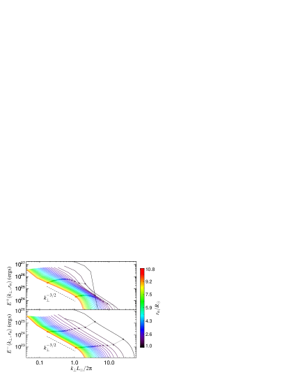
Figure 6.— Radial evolution of the steady state energy spectra for simulation E2 in table  1.

Figure 6 shows $E^{\pm}(k_{\perp},r_{n})$ for simulation E2 for selected $r_{n}$ values ranging from $1.01R_{\sun}$ to $11.09R_{\sun}$. If we were to plot $E^{\pm}(k_{\perp},r_{n})$ versus $\tilde{k}_{\perp}=k_{\perp}L_{\perp}(r)/2\pi$, the spectra at different $r_{n}$ would all cover the same range of $\tilde{k}_{\perp}$ values. However, in Figure 6 we plot $E^{\pm}$ versus $k_{\perp}L_{\perp\sun}/2\pi$, and thus the spectra migrate to the left as $r$ increases. The spectra extend over the wavenumber range $1\leq\tilde{k}_{\perp}\lesssim 85$ rather than the range $1\leq\tilde{k}_{\perp}\leq 128$, because we set $\Omega^{\pm}_{\alpha\tilde{k}_{x}\tilde{k}_{y},n}=0$ when $\tilde{k}_{\perp}>N_{\perp}/3$ in order to dealias the simulations, where $\tilde{k}_{\perp}$ is defined in Equation (17).

Because all the energy is injected through the lower boundary and into wavevectors in the range $1\leq\tilde{k}_{\perp}\leq 3$, all fluctuations on scales $\tilde{k}_{\perp}\geq 4$ are the result of the nonlinear interaction between $z^{+}$ fluctuations and the $z^{-}$ fluctuations that are produced by reflection. As Figure 6 illustrates, the fluctuations develop power-law-like spectra over the wavenumber interval $4\lesssim\tilde{k}_{\perp}\lesssim 25$ at all locations except the immediate vicinity of $r=R_{\sun}$. We determine the spectral index $\alpha_{n}^{\pm}$ of the $z^{\pm}$ power spectrum in the $n^{\rm th}$ radial subdomain by fitting $E^{\pm}(k_{\perp},r_{n})$ to a power law of the form

$$E^{\pm}(k_{\perp},r_{n})\propto k_{\perp}^{-\alpha_{n}^{\pm}}$$ (38)

over the wavenumber interval $4<\tilde{k}_{\perp}<25$. Figure  7 shows how $\alpha_{n}^{\pm}$ depends upon $r_{n}$ for the ten simulations listed in Table 1. Although the large-scale $z^{+}$ eddies injected at the base of the corona result in vanishing wave power at $\tilde{k}_{\perp}>4$ at $r=r_{\rm min}$, there is a non-negligible amount of power at $\tilde{k}_{\perp}>4$ in $E^{\pm}(k_{\perp},r_{1})$ because of the domain averaging procedure in Equation (36), which averages the strictly large-scale spectrum at $r=r_{\rm min}$ with the energy spectrum that develops at slightly larger radii within the first domain, which extends out to a maximum radius of $\simeq 1.02R_{\sun}$. The high-$k_{\perp}$ $z^{+}$ fluctuations at small $r$ arise in part from the cascade of $z^{+}$ fluctuations and in part from the reflection of broad-spectrum $z^{-}$ fluctuations at small $r$ (Verdini et al., 2009, 2012). We discuss the dependence of $\alpha^{\pm}_{n}$ on $r_{n}$, $L_{\perp\sun}$, and $\tau_{\rm c\sun}^{+}$ in Section V .

Figure 7.— Radial dependence of the spectral indices $\alpha^{\pm}$ of the $E^{\pm}$ energy spectra for simulations A1 to E1 (left) and simulations A2 to E2 (right).

IV.4. Heating Rates and Energy Conservation

We obtain a steady-state energy-conservation relation by taking the dot product of Equation (6) with $\rho\mathbf{z}^{\pm}$, adding the resulting equations for $\rho(\partial/\partial t)(z^{+})^{2}/2$ and $\rho(\partial/\partial t)(z^{-})^{2}/2$, and dividing by 2. We then integrate over the simulation volume and average over time to obtain

$$F_{\sun}^{+}=F_{\rm A}^{+}+|F^{-}_{\sun}|+W_{\rm bg}+Q,$$ (39)

where $F_{\sun}^{\pm}=F^{\pm}(R_{\sun})$, $F_{\rm A}^{+}=F^{+}(r_{\rm A})$, and

$$F^{\pm}(r)=\rho a\left(U\pm v_{\rm A}\right)u^{\pm}$$ (40)

is the area-integrated $z^{\pm}$ energy flux through the flux-tube cross section at heliocentric distance $r$. The quantities $u^{\pm}$ and $a$ are defined in Equations (32) and (37), $u_{\rm R}\equiv\left\langle\mathbf{z}^{+}\cdot\mathbf{z}^{-}\right\rangle/2$ is the residual energy density per unit mass, and

$$W_{\rm bg}=\int dr\rho aU\left(\frac{u^{+}+u^{-}}{2H_{\rho}}-\frac{u_{\rm R}}{H_{\rm A}}\right)$$ (41)

is the rate at which the fluctuations do work on the background flow (e.g. solar-wind acceleration by the magnetic pressure of the AWs). The term

$$Q=\int_{\rm r_{\rm min}}^{r_{\rm max}}dr\rho a(q^{+}+q^{-})$$ (42)

is the total turbulent heating rate integrated over the simulation volume,

$$q^{\pm}(r)=\frac{1}{2}\nu_{p}\langle|{\bf T}^{\pm}|^{2}\rangle$$ (43)

is the $z^{\pm}$ dissipation power per unit mass at radius $r$ due to hyperviscosity, and

$$|{\bf T}^{\pm}|^{2}=\sum_{i_{1}=1}^{2}\sum_{i_{2}=1}^{2}\dots\sum_{i_{p}=1}^{2}\sum_{j=1}^{2}\big{[}\left(\nabla_{\perp}\right)_{i_{1}}\cdots\left(\nabla_{\perp}\right)_{i_{p}}z^{\pm}_{j}\big{]}\big{[}$$

$$\left(\nabla_{\perp}\right)_{i_{1}}\cdots\left(\nabla_{\perp}\right)_{i_{p}}z^{\pm}_{j}\big{]},$$ (44)

where $\left(\nabla_{\perp}\right)_{1}=\partial/\partial x$, $\left(\nabla_{\perp}\right)_{2}=\partial/\partial y$, $z^{\pm}_{1}=\mathbf{e}_{x}\cdot\mathbf{z}^{\pm}$, and $z^{\pm}_{2}=\mathbf{e}_{y}\cdot\mathbf{z}^{\pm}$.

We refer to $F^{+}_{\sun}$ as the “input power” and the time integral of $F^{+}_{\sun}$ as the “input energy.” In Figure 8 we plot the quantities $F^{+}_{\rm A}/F^{+}_{\sun}$, $|F^{-}_{\sun}|/F^{+}_{\sun}$, $W_{\rm bg}/F^{+}_{\sun}$, and $Q/F^{+}_{\sun}$. Equation (39) implies that in steady state these fractions add to one. In our simulations, these fractions add to $1\pm 0.03$. The small deviations from unity are expected because time averages in our finite-duration simulations are only approximations of a statistical steady state. In Simulations A1 through E1, the largest single “sink” of input energy is the work done on the background flow, although comparable amounts of energy go into turbulent heating and the $z^{+}$ energy that escapes through the outer boundary at $r=r_{\rm A}$. In Simulations A2 through E2, the larger value of $L_{\perp}$ systematically weakens turbulent dissipation relative to simulations A1 through E1, and the fraction of the input power that goes into turbulent heating is reduced to values $\sim 0.15-0.25$.

Figure 8.— The fractions of the $z^{+}$ input energy at $r=R_{\sun}$ that escapes as $z^{+}$ energy at $r=r_{\rm A}$ (solid line), escapes as $z^{-}$ energy at $r=R_{\sun}$ (dashed line), that goes into work on the background flow (dash-dot-dash line), and that goes into turbulent heating (dash-triple-dot-dash line).

In Figure 9 we plot $q^{+}(r)$ and $q^{-}(r)$ for the simulations in Table 1. Even though we have launched only large-scale AWs at $r=R_{\sun}$, these waves undergo a vigorous cascade leading to heating rates $\gtrsim 10^{10}\mbox{ cm}^{3}\mbox{ s}^{-1}$ between $2R_{\sun}$ and $11R_{\sun}$. The reason that $q^{+}$ decreases as $r$ decreases from $2R_{\sun}$ to $R_{\sun}$ is that it takes time for the $z^{+}$ fluctuations entering the domain at $r=R_{\sun}$ to cascade from the injection lengthscale $\sim L_{\perp}$ to the dissipation scale $d$, and the $z^{+}$ fluctuations move away from the Sun during this time. The radius $r_{\rm q}$ at which $q^{+}$ reaches its maximum value is larger in the simulations with $L_{\perp\sun}=2\times 10^{4}\mbox{ km}$ than in the simulations with $L_{\perp\sun}=10^{4}\mbox{ km}$ because the energy-cascade timescales increase with increasing $L_{\perp\sun}$. The value of $r_{\rm q}$ also depends on the dissipation scale $d$. In a hypothetical simulation with much higher numerical resolution and much smaller hyperviscosity, $d$ would be smaller, it would take longer for energy to cascade from scale $L_{\perp}$ to scale $d$, and $r_{\rm q}$ would increase. On the other hand, in many models of turbulence the energy-cascade timescale decreases with scale, in which case decreasing $d$ would have only a modest effect on the total energy cascade time. If we were to launch a broad spectrum of $z^{+}$ AWs into the simulation domain at $r=r_{\rm min}$, the AWs launched at perpendicular wavenumbers satisfying $L_{\perp}^{-1}\ll k_{\perp}\ll d^{-1}$ would require less time to cascade to scale $d$, leading to additional heating close to the Sun’s surface. The radial profile of $q^{+}$ in the region $R_{\sun}<r<2R_{\sun}$ is thus sensitive to the assumed $k_{\perp}$ spectrum of the waves launched by the Sun $e^{+}(k_{\perp},R_{\sun})$. Future investigations into the dependence of $q^{+}(r)$ on $e^{+}(k_{\perp},R_{\sun})$ will be important for determining the radial profile of the heating rate at small $r$.

We note that $q^{+}\gg q^{-}$ at $r\gtrsim 2R_{\sun}$ because there is more $z^{+}$ energy than $z^{-}$ energy. On the other hand, $q^{-}\gg q+$ very close to $r=r_{\rm min}$, because there is very little $z^{+}$ energy at large $k_{\perp}$ due to the steepness of the $z^{+}$ power spectrum near the coronal base.

The peak heating rates of $\sim 10^{10}\mbox{ cm}^{2}\mbox{ s}^{-3}$ to $\sim 3\times 10^{10}\mbox{ cm}^{2}\mbox{ s}^{-3}$ in our simulations are smaller than the peak heating rates of $\sim\times 10^{11}\mbox{ cm}^{2}\mbox{ s}^{-3}$ to $\sim\times 10^{12}\mbox{ cm}^{2}\mbox{ s}^{-3}$ in the wave-driven solar-wind models of Cranmer et al. (2007), Verdini et al. (2010), and Chandran et al. (2011). One reason for this difference is that the rms wave amplitudes in our simulations are smaller than in these models. We do not conclude that the peak values of $q^{\pm}$ in our simulations are more accurate than in these previous models, because of the uncertainty in the correct value of $z^{+}_{\rm rms}$ at the coronal base (see discussion at the beginning of Section IV), and to a lesser degree because of uncertainties in the background solar-wind profiles.

Dmitruk and Matthaeus (2003) conjectured that turbulent heating in coronal holes at $R_{\sun}<r<2R_{\sun}$ is favored when the inequalities $\tau_{\rm nl}^{-}<\tau_{\rm r}<R_{\sun}/\langle v_{\rm A}\rangle<\tau_{\rm c\,\sun}^{+}<t_{\eta}$ are satisfied, where $t_{\eta}$ is the resistive timescale at scale $L_{\perp}$, and $\langle v_{\rm A}\rangle$ is the average value of $v_{\rm A}$ between $r=R_{\sun}$ and $r=2R_{\sun}$. Most of these inequalities are at least marginally satisfied in our simulations at $r<2R_{\sun}$. The exception is that the inequality $R_{\sun}/\langle v_{\rm A}\rangle<\tau_{\rm c\,\sun}^{+}$ is violated when when $\tau_{\rm c\,\sun}^{+}\lesssim 5.84\mbox{ min}$. The fact that the heating rates at $1.5R_{\sun}\lesssim r<2R_{\sun}$ are lower in Simulations D1, D2, E1 and E2 than in the other simulations is thus consistent with Dmitruk & Matthaeus’ (2003) conjecture.

The dependence of $q^{+}$ on $\tau_{\rm c,\sun}^{+}$, however, reverses as $r$ increases to values exceeding $\sim 2.5R_{\sun}$. As shown in Figures 8 and 9, runs with larger $\tau_{\rm c\sun}^{+}$ have smaller heating rates at $r\gtrsim 2.5R_{\sun}$, despite the fact that $z^{-}_{\rm rms}$ is larger. In Section VI, we describe how this result can be understood by considering an effect that systematically weakens nonlinear interactions at $r\gtrsim 2.5R_{\sun}$ as $\tau_{\rm c\,\sun}^{+}$ is increased.

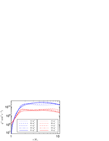
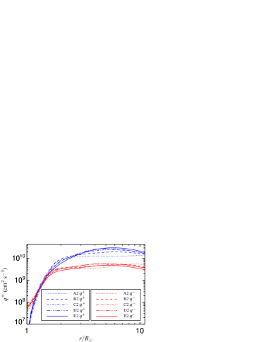
Figure 9.— Heating-rate profiles $q^{\pm}(r)$ (defined in Equation (43)). Left panel: Simulations A1 through E1, in which $L_{\perp 0}=10^{4}~{}\mbox{ km}$. Right panel: Simulations A2 through E2, in which $L_{\perp\sun}=2\times 10^{4}\mbox{ km}$.

V. Anomalous $z^{-}$ Fluctuations and the $k^{-1}$ Spectrum of the Interplanetary Magnetic Field

One of the most important ideas in the study of reflection-driven turbulence is the distinction between “classical” and “anomalous” $z^{-}$ fluctuations (Velli et al., 1989; Verdini et al., 2009, 2012). After a $z^{-}$ fluctuation is produced by reflection, it propagates towards the Sun at speed $v_{\rm A}$ in the reference frame of the solar wind. However, because the sources of the $z^{-}$ fluctuations are $z^{+}$ fluctuations that propagate away from the Sun in the solar-wind frame, if one views the pattern of $z^{-}$ fluctuations, some component of that pattern propagates away from the Sun along with $z^{+}$. This component of the $z^{-}$ wave field is the anomalous component. The remainder of the $z^{-}$ wave field is the classical component.

The anomalous $z^{-}$ fluctuations play an important role because they coherently shear the $z^{+}$ fluctuations that produce them. This effect is absent in homogeneous RMHD turbulence and alters the phenomenology of the energy cascade. In homogeneous RMHD turbulence, nonlinear interactions proceed through a series of collisions between counter-propagating $z^{+}$ and $z^{-}$ wave packets. Successive collisions are uncorrelated, and so if the wave amplitudes are sufficiently small, the effects of successive collisions add incoherently as in a random walk (Kraichnan, 1965), leading to a weak-turbulence regime with a slow energy cascade (Ng and Bhattacharjee, 1996, 1997; Galtier et al., 2000). In contrast, when a $z^{+}$ wave packet is sheared by the “anomalous” $z^{-}$ fluctuations produced by the reflection of that $z^{+}$ wave packet, the shearing is coherent in time, which strengthens the nonlinear interaction relative to the homogeneous case.

Velli et al. (1989) argued that an energy cascade driven by anomalous $z^{-}$ fluctuations leads to an inertial-range $z^{+}$ power spectrum that is much flatter than in homogeneous turbulence. They considered fluctuations with an isotropic wavenumber spectrum and estimated the magnitude of the source term for anomalous $z^{-}$ fluctuations at wavenumber $k$ to be $z^{+}_{k}/\tau_{\rm r}$, where $z^{+}_{k}$ is the rms amplitude of the $z^{+}$ fluctuations at perpendicular scale $k^{-1}$. They multiplied this source term by the time it takes for $z^{-}$ fluctuations to propagate away from their source, which is $\sim(kv_{\rm A})^{-1}$, to obtain the estimate $z^{-}_{k,\rm a}\sim z^{+}_{k}/(kv_{\rm A}\tau_{\rm r})$, where $z^{-}_{k,\rm a}$ is the rms amplitude of anomalous $z^{-}$ fluctuations at scale $k^{-1}$. Upon taking the $z^{+}$ cascade power

$$\epsilon^{+}\sim kz_{k,\rm a}^{-}(z_{k}^{+})^{2}$$ (45)

to be independent of $k$, they found that $z_{k}^{+}$ becomes independent of $k$, leading to a $k^{-1}$ inertial-range power spectrum for $z^{+}$. Since $z^{+}$ dominates the fluctuation energy, the $k^{-1}$ spectrum for $z^{+}$ implies a $k^{-1}$ spectrum for the magnetic field, velocity field, and fluctuation energy.

The arguments of Velli et al. (1989) can be revised to account for wavenumber anisotropy and the shearing of $z^{-}$ fluctuations by $z^{+}$ fluctuations. If the fluctuations vary much more rapidly in the directions perpendicular to $\mathbf{B}_{0}$ than in the direction parallel to $\mathbf{B}_{0}$ (the “quasi-2D” case), then we can replace $k$ with $k_{\perp}$ in the arguments of Velli et al. (1989), defining $z_{k_{\perp}}^{+}$ to be the rms amplitude of $z^{+}$ fluctuations at perpendicular scale $k_{\perp}^{-1}$, and $z^{-}_{k_{\perp},\rm a}$ to be the rms amplitude of anomalous $z^{-}$ fluctuations at perpendicular scale $k_{\perp}$. The source term for the production of $z^{-}$ by the reflection of $z^{+}$ at scale $k_{\perp}^{-1}$ is $S_{k_{\perp}}\sim z^{+}_{k_{\perp}}/\tau_{\rm r}.$ The $z^{-}$ fluctuations at perpendicular scale $k_{\perp}$ cascade to smaller scales in a time $t_{k_{\perp}}\sim(k_{\perp}z^{+}_{k_{\perp}})^{-1}$. If this cascade time is shorter than the wave period, then $z^{-}_{k_{\perp},\rm a}$ is approximately equal to the product of $S_{k_{\perp}}$ and $t_{k_{\perp}}$; i.e., $z^{-}_{k_{\perp},\rm a}\sim(k_{\perp}\tau_{\rm r})^{-1}$. Equation (45) (with $k$ replaced by $k_{\perp}$) then yields the relation

$$\epsilon^{+}\sim(z_{k_{\perp}}^{+})^{2}/\tau_{\rm r}.$$ (46)

Taking $\epsilon^{+}$ to be independent of $k_{\perp}$ implies that $z_{k_{\perp}}^{+}$ is independent of $k_{\perp}$. The $z^{+}$ energy per unit $k_{\perp}$, roughly $(z_{k_{\perp}}^{+})^{2}/k_{\perp}$, is then again $\propto k_{\perp}^{-1}$.

The above arguments suggest that $E^{+}$ evolves towards a $k^{-1}$ scaling (or a $k_{\perp}^{-1}$ scaling in the case of quasi-2D turbulence) when the anomalous component of $z^{-}$ dominates the nonlinear shearing of the $z^{+}$ fluctuations, and that $E^{+}$ is similar to the spectrum of homogeneous RMHD turbulence, in which $\alpha^{+}\approx 3/2$, when the classical component of $z^{-}$ dominates the nonlinear shearing of the $z^{+}$ fluctuations. To explain the behavior of the power spectra in our simulations, we would need to explain the relative contributions of anomalous and classical $z^{-}$ fluctuations to the shearing of $z^{+}$ at each scale, which is beyond the scope of this paper. We instead confine ourselves to the following observations.

Figure 10.— Alignment angles for the Elsässer potentials $\phi^{\pm}$ and outer-scale vorticity $\Omega^{\pm}_{0}$, which excludes contributions to $\Omega^{\pm}$ from $\tilde{k}_{\perp}>2$. The left panel corresponds to simulations A1 through E1, and the right panel to Simulations A2 through E2.

The flat spectra in our simulations arise in two distinct regimes. First, in the large-$\tau_{\rm\,\sun}^{+}$ runs A1, A2, and B1, $\alpha^{+}$ decreases to values of $1.3-1.4$ at $3R_{\sun}<r<4R_{\sun}$. These flat spectra are in some ways reminiscent of the $z^{+}$ spectrum found by Verdini et al. (2009) in numerical simulations of reflection-driven AW turbulence in which the nonlinear terms in Equation (6) were approximated using a shell model. In their simulations, $\alpha^{+}\sim 1.2$ at $r\lesssim 1.2R_{\sun}$, but at larger radii the $z^{+}$ spectrum steepened towards $\alpha^{+}=5/3$. Second, in our smallest-$\tau_{\rm c\,\sun}^{+}$ simulations (E1 and E2), the spectrum becomes increasingly flat as $r$ increases. The clearest evolution towards a $k_{\perp}^{-1}$ spectrum occurs in Simulation E2, in which $\alpha^{+}$ decreases almost linearly with $\ln(r)$, reaching the value $\alpha^{+}=1.3$ at $r=11.1R_{\sun}$. The upper-right-hand panel of Figure 7 suggests that $\alpha^{+}$ would reach even smaller values in Simulation E2 if we were to extend that simulation to larger $r$.

A characteristic that sets Simulations E1 and E2 apart from the other simulations is that the $z^{-}$ cascade becomes weak at large $r$. This can be seen from the bottom panels of Figure 4, which show that $\tau_{\rm c}^{+}<\tau_{\rm nl}^{-}$ at large $r$ in simulations E1 and E2. This inequality means that outer-scale $z^{+}$ fluctuations decorrelate in less time than the time it takes them to significantly distort the outer-scale $z^{-}$ fluctuations. As a consequence, the effects on $z^{-}$ of successive collisions between outer-scale wave packets accumulate in a random-walk-like manner, which slows down the $z^{-}$ energy cascade. Another characteristic that distinguishes Simulations E1 and E2 is the lack of alignment between contours of constant $\phi^{+}$ and contours of constant (outer-scale) $\Omega^{+}$, as illustrated in the bottom panel of Figure 10. As we discuss further in Section VI, the alignment between these contours that arises in the other simulations acts to weaken the nonlinear interactions arising from anomalous $z^{-}$ fluctuations.

The flat spectra in Simulations E1 and E2 may be relevant to the magnetic power spectrum $E_{B}(k)$ observed in the interplanetary medium. Spacecraft measurements show that the power spectrum at small wavenumbers (i.e., neglecting the dissipation range) has a broken-power-law form, with $E_{B}(k)\propto k^{-n_{1}}$ at $k<k_{\rm br}$ and $E_{B}(k)\sim k^{-n_{2}}$ at $k>k_{\rm br}$, where $n_{1}\simeq 1$ and $n_{2}\simeq 5/3$ (Matthaeus and Goldstein, 1986; Tu and Marsch, 1995). Moreover, $k_{\rm br}$ increases as $r$ decreases from 1 AU to 0.3 AU (Bruno and Carbone, 2005). The results of Simulations E1 and E2 support the suggestion of Velli et al. (1989) that reflection-driven turbulence can give rise to a $k^{-1}$ scaling of $E_{B}$ over at least some ranges of $k$ and $r$. Our results, however, are not fully conclusive on this point because the wavenumber spectrum of $z^{+}$ at large $r$ depends upon the frequency spectrum of $z^{+}$ at the coronal base, which is uncertain. Cranmer and van Ballegooijen (2005) analyzed time series of the observed positions of magnetic bright points (MBPs) on the Sun and found that MBP motions had dominant timescales of $1-10\mbox{ min}$. The timescales of photospheric motions, however, may be larger than the timescale $\tau_{\rm c\,\sun}^{+}$ characterizing outer-scale fluctuations at the coronal base. Van Ballegooijen et al (2011) carried out numerical simulations of AW turbulence from the photosphere to the corona. They found that when large-scale waves are launched from the photosphere, these waves become fully turbulent within the chromosphere, before reaching the transition region. This causes the outer-scale fluctuations in their simulations to vary on a timescale that is significantly shorter in the corona than at the photosphere (see their Figure 8c). On the other hand, fluctuations in the Faraday rotation of radio signals passing near the Sun suggest that the outer-scale magnetic fluctuations at $2R_{\sun}\lesssim r\lesssim 15R_{\sun}$ vary on timescales of $\sim 1\mbox{ hr}$ (Hollweg, 1982). Pinning down the frequency spectrum of the waves at the coronal base and incorporating broad-spectrum AW launching into numerical simulations such as the ones presented here will be important for clarifying the possible connection between reflection-driven turbulence and the $k^{-1}$ power spectra observed in the solar wind.

VI. Vorticity-Potential Alignment

The nonlinear term on the right-hand side of Equation (LABEL:eq:vorticity), $\mathcal{N}^{\pm}\equiv-\mathbf{\hat{b}}\cdot\left[\nabla_{\perp}\times\left(\mathbf{z}^{\mp}\cdot\nabla_{\perp}\mathbf{z}^{\pm}\right)\right]$, is responsible for the transfer of energy from large scales to small scales. This term can be written in the form (Schekochihin et al., 2009)

$$\mathcal{N}^{\pm}=\frac{1}{2}\left(\left[\Omega^{+},\phi^{-}\right]+\left[\Omega^{-},\phi^{+}\right]\pm\nabla_{\perp}^{2}\left[\phi^{+},\phi^{-}\right]\right),$$ (47)

where

$$\left[f,g\right]\equiv\mathbf{e}_{z}\cdot\left(\nabla_{\perp}f\times\nabla_{\perp}g\right)$$ (48)

is the Poisson bracket for arbitrary scalar functions $f$ and $g$. These equations show that the shearing of $\mathbf{z}^{\pm}$ by $\mathbf{z}^{\mp}$ is related to the angle between $\nabla_{\perp}\phi^{+}$ and $\nabla_{\perp}\phi^{-}$, the angle between $\nabla_{\perp}\Omega^{+}$ and $\nabla_{\perp}\phi^{-}$, and the angle between $\nabla_{\perp}\Omega^{-}$ and $\nabla_{\perp}\phi^{+}$. We define the characteristic alignment angle $\theta(f,g)$ for the scalar functions $f$ and $g$ through the equation

$$\theta(f,g)=\sin^{-1}\left(\frac{\left\langle\left|\nabla_{\perp}f\times\nabla_{\perp}g\right|\right\rangle}{\left\langle\left|\nabla_{\perp}f\right|\left|\nabla_{\perp}g\right|\right\rangle}\right),$$ (49)

where $\langle\dots\rangle$ denotes an average over $x$, $y$, and $t$. From equation (47) it follows that the angles $\theta(\phi^{\pm},\Omega^{\mp})$ and $\theta(\phi^{+},\phi^{-})$ are intimately related to the strength of the interaction between $z^{\pm}$ fluctuations, therefore it is natural to expect that any decrease in these angles results in a weakening of nonlinear interactions.

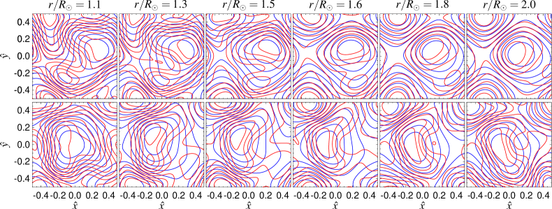
Figure 11.— Contours of constant $\phi^{+}$ (blue line) and constant $\Omega_{0}^{+}$ (red line) in field-perpendicular planes at selected radii ($r/R_{\sun}=1.1,1.3,1.5,1.6,1.8,2.0$). The top panels correspond to simulation A1 and the bottom panels corresponds to simulation D1. The contours of $\phi^{+}$ and $\Omega_{0}^{+}$ clearly become more aligned at larger values of $\tau_{\rm c\sun}$. In these plots $\hat{x}=x/L_{\perp}(r)$ and $\hat{y}=y/L_{\perp}(r)$.

Figure 10 shows the alignment angles $\theta(\phi^{+},\phi^{-})$, $\theta(\Omega_{0}^{+},\phi^{-})$, $\theta(\Omega_{0}^{-},\phi+)$, and $\theta(\Omega_{0}^{+},\phi^{+})$ as functions of $r$ for the runs in Table 1, where $\Omega_{0}^{\pm}$ is the value of $\Omega^{\pm}$ after we have filtered out the contributions from $\tilde{k}_{\perp}>2$. This filtering process allows us to focus on the alignment angles that characterize nonlinear interactions between outer-scale fluctuations. In the absence of filtering, $\Omega^{\pm}$ is dominated by the largest $k_{\perp}$ values in the inertial range, which we assume have little effect upon the energy cascade at scales $\sim L_{\perp}$.

As $r$ increases from $R_{\sun}$ to $3R_{\sun}$, these angles decrease, to a degree that increases as $\tau_{\rm c\,\sun}$ increases. The alignment angles are $\sim 2-4$ times smaller in Simulation A1 than in Simulation E1. On the other hand, $z^{-}_{\rm rms}$ is $2-3$ times smaller in Simulation E1 than in Simulation A1. Vorticity-potential alignment thus helps to explain why $q^{+}$ is a decreasing function of $\tau_{\rm c\,\sun}^{+}$ at $3R_{\sun}\lesssim r\lesssim 10R_{\sun}$, despite the fact that $z^{-}_{\rm rms}$ is an increasing function of $\tau_{\rm c\,\sun}^{+}$.

The dependence of alignment on $\tau_{\rm c\,\sun}^{+}$ derives in part from the linear physics of wave reflection. The source term in Equation (LABEL:eq:vorticity) representing the production of $\Omega^{-}$ by wave reflection has the form $-(U+v_{\rm A})\Omega^{+}/2H_{\rm A}$. The structure of this term in the $x-y$ plane is identical to the structure of $\Omega^{+}$, and thus reflection acts to produce an $\Omega^{-}$ field that is locally “aligned” with $\Omega^{+}$, in the sense that $\theta(\Omega^{+},\Omega^{-})$ is small. For the same reason, reflection acts to produce a $\phi^{-}$ field that is locally aligned with $\phi^{+}$, and an $\Omega_{0}^{-}$ field that is aligned with $\Omega_{0}^{+}$. After $z^{-}$ fluctuations are produced by wave reflection, they propagate towards the Sun at speed $v_{\rm A}$ in the plasma frame, separating from the $z^{+}$ fluctuation that produced them. This separation acts to decrease the alignment between $\phi^{+}$ and $\phi^{-}$ and becomes more important as $\tau_{\rm c\,\sun}$ decreases, since the radial lengthscales of the fluctuations become shorter, enabling $z^{-}$ fluctuations to separate from their sources more rapidly.

The bottom panel of Figure 10 shows the alignment angle between $\phi^{+}$ and $\Omega_{0}^{+}$. This angle does not characterize any of the terms in Equation (47), and so is not a direct measure of the efficiency of nonlinear interactions. Instead, the decrease in $\theta(\phi^{+},\Omega_{0}^{+})$ with increasing $r$ in Simulations A1 through D1 and A2 through D2 can be characterized as the decay of $z^{+}$ fluctuations towards a state of “vorticity-potential alignment.” As the fluctuations approach a state in which $\theta(\phi^{+},\Omega_{0}^{+})=0$, the outer-scale $z^{-}$ fluctuations produced by wave reflection become increasingly inefficient at shearing outer-scale $z^{+}$ fluctuations and are in turn sheared increasingly inefficiently by the outer-scale $z^{+}$ fluctuations. The radial decay of $\theta(\phi^{+},\Omega_{0}^{+})$ weakens as $\tau_{\rm c\,\sun}^{+}$ decreases. One reason for this is likely that $z^{-}_{\rm rms}$ also decreases with decreasing $\tau_{\rm c\,\sun}^{+}$, so that the “selective decay” of the unaligned component of $z^{+}$ proceeds more slowly. The dependence of $\theta(\phi^{+},\Omega_{0}^{+})$ on $r$ and $\tau_{\rm c,\sun}^{+}$ is illustrated in Figure 11, which plots contours of $\phi^{+}$ and $\Omega_{0}^{+}$ at selected radii between $1R_{\sun}$ and $2R_{\sun}$ in Simulations A1 and D1.

VII. Summary and Conclusion

We have carried out the first direct numerical simulations of inhomogeneous RMHD turbulence from the coronal base to the Alfvén critical point that take into account radial variations in $U$, $\rho$, and $B_{0}$ without approximating the nonlinear terms in the inhomogeneous RMHD equations. The simulation domain is a magnetic flux tube with a square cross section of area $L_{\perp}(r)^{2}$ that extends from $r=R_{\sun}$ to $r=r_{\rm A}=11.1R_{\sun}$, the location of the Alfvén critical point in our model solar wind. This flux tube is narrow, with $L_{\perp}\ll r$ at all $r$.

There are three control parameters in the simulations: the rms amplitude of $z^{+}$ at the coronal base, denoted $z^{+}_{\rm rms\,\sun}$, the correlation time of the outer-scale $z^{+}$ fluctuations at the coronal base, denoted $\tau_{\rm c\,\sun}^{+}$, and the width of the cross section of the simulation domain at the coronal base, denoted $L_{\perp\sun}$. For the ten simulations reported in this study, we choose $z^{+}_{\rm rms\,\sun}$ so that the rms velocity at $r=R_{\sun}$ is $\simeq 20\mbox{ km/s}$. We take $L_{\perp\sun}$ to be either $10^{4}\mbox{ km}$ or $2\times 10^{4}\mbox{ km}$, comparable to the spatial scales of supergranules. We consider $\tau_{\rm c\,\sun}^{+}$ values ranging from $2\mbox{ min}$ to $20\mbox{ min}$. (A smaller value of $\tau_{\rm c\,\sun}^{+}$ implies higher wave frequencies, which reduces the efficiency of wave reflection.)

The $z^{+}$ AWs that we launch through the simulation boundary at $r=R_{\sun}$ have small perpendicular wavenumbers  $\sim 2\pi/L_{\perp\,\sun}$. As the $z^{+}$ fluctuations propagate away from the Sun, they undergo partial non-WKB reflection, which generates $z^{-}$ fluctuations. Nonlinear interactions between $z^{+}$ fluctuations and $z^{-}$ fluctuations causes fluctuation energy to cascade to small scales and dissipate, heating the ambient plasma. Between 15% and 33% of the $z^{+}$ energy launched by the Sun (the “input energy”) dissipates within the simulation domain, between 33% and 40% goes into work on the background flow, and between 22% and 36% escapes as $z^{+}$ energy at $r=r_{\rm A}$, for all input parameters investigated in this work. Our finding that $\sim 1/6-1/3$ of the input energy dissipates at $r<r_{\rm A}$ is consistent with Chandran & Hollweg’s (2009) analytical model of reflection-driven turbulence in the solar wind, which finds (their Equation 43) that the outer-scale $z^{+}$ fluctuations experience an order-unity number of cascade times as they propagate from the coronal base to the Alfvén critical point, without any fine-tuning of parameters. These results provide an important consistency check on models in which the solar wind is powered by AWs and AW turbulence. If only a tiny fraction of the input energy were dissipated at $r<r_{\rm A}$, then AW turbulence would be unable to explain the powerful heating rates that are inferred from observations of ion temperature profiles in coronal holes (Kohl et al., 1998; Esser et al., 1999). If almost all of the input energy were dissipated, then the wave amplitudes and heating rates near the Sun would have to be unrealistically large in order that enough energy would survive to explain the large amplitudes of outward-propagating $z^{+}$ fluctuations observed at $r\sim 0.3\mbox{ AU}$.

As the $z^{+}$ fluctuations propagate away from the Sun, their power spectrum gradually flattens towards power a power law of the form $E^{+}(k_{\perp})\propto k_{\perp}^{-\alpha^{+}}$, where $1.3\lesssim\alpha^{+}\lesssim 2.4$. Velli et al. (1989) argued that reflection-driven turbulence gives rise to a $k^{-1}$ power spectrum for the $z^{+}$ fluctuations, which could potentially explain the $k^{-1}$ magnetic power spectrum observed at large scales in the solar wind. In our Simulation E2, $\alpha^{+}$ decreases steadily with increasing $r$, reaching a value of $1.3$ at $r=11.1R_{\sun}$. The steady decline of $\alpha^{+}$ with increasing $r$ suggests that the spectrum would become even flatter if we were to extend the simulation to larger $r$. In Simulation E2, $L_{\perp\sun}=2\times 10^{4}\mbox{ km}$ and $\tau_{\rm c\,\sun}^{+}=2\mbox{ min}$. Similar behavior is seen in the $z^{+}$ spectrum in Simulation E1 in which $L_{\perp\sun}=10^{4}\mbox{ km}$ and $\tau_{\rm c\,\sun}^{+}=2\mbox{ min}$, but the spectral flattening is less pronounced. In our other simulations with larger values of $\tau_{\rm c\,\sun}^{+}$, the spectra at large $r$ are steeper. The ability of reflection-driven turbulence to explain the $k^{-1}$ spectra in the solar wind thus depends upon the frequency and wavenumber spectra of the $z^{+}$ AWs launched by the Sun, as well as upon the evolution of the fluctuations at $r>r_{\rm A}$.

In the simulations that we have run with $\tau_{\rm c\,\sun}^{+}\geq 3.3\mbox{ min}$, the fluctuations develop a type of alignment between the contours of constant $\phi^{+}$, $\phi^{-}$, $\Omega_{0}^{+}$, and $\Omega_{0}^{-}$, where $\Omega_{0}^{\pm}$ is the contribution to $\Omega^{\pm}$ from the outer-scale fluctuations, and $\phi^{\pm}$ and $\Omega^{\pm}$ are the Elsässer potential and Elsässer vorticity defined in Equations (12) and (13). In Simulations A1 through D1 and A2 through D2, these angles decrease between $r=R_{\sun}$ and $r\sim 2R_{\sun}$, which causes nonlinear interactions to weaken. This effect becomes increasingly pronounced as $\tau_{\rm c\,\sun}^{+}$ increases, and helps to explain why the turbulent heating rate at $r\gtrsim 3R_{\sun}$ decreases with increasing $\tau_{\rm c\,\sun}^{+}$ despite the fact that $z^{-}_{\rm rms}$ increases, as shown in Figure 9.

Our simulations with $L_{\perp\sun}=10^{4}\mbox{ km}$ are broadly similar to our simulations with $L_{\perp\sun}=2\times 10^{4}\mbox{ km}$. Since the perpendicular correlation length of the turbulence in our simulations is $\simeq L_{\perp}$, our simulations show that modest changes in this perpendicular correlation length lead to only moderate changes in the properties of reflection-driven turbulence between the Sun and the Alfvén critical point. On the other hand, it is possible that values of $L_{\perp\sun}$ much smaller than $10^{4}\mbox{ km}$ would lead to significantly different results, and future simulations to investigate this possibility would be useful.

Another useful direction for future research would be to carry out simulations in which a broad spectrum of waves is launched at $r=R_{\sun}$. More work is also needed to clarify the phenomenology of reflection-driven turbulence, to explain the different types of power spectra that it produces, and to determine whether it provides a viable explanation for at least some portion of the $k^{-1}$ magnetic power spectrum observed at small $k$ in the solar wind. Finally, it will be informative to compare the results of simulations such as the ones presented here with future measurements from the Solar Probe Plus spacecraft, which has a planned perihelion of $9.5R_{\sun}$ that lies inside the region that we are simulating numerically. Such comparisons will be useful for testing theories of reflection-driven AW turbulence and clarifying the role played by AW turbulence in the origin of the solar wind.

References

- Coleman (1968) P. J. Coleman, ApJ 153, 371 (1968).
- Belcher and Davis (1971) J. W. Belcher and L. Davis, Jr., J. Geophys. Res. 76, 3534 (1971).
- Coles and Harmon (1989) W. A. Coles and J. K. Harmon, ApJ 337, 1023 (1989).
- Bale et al. (2005) S. D. Bale, P. J. Kellogg, F. S. Mozer, T. S. Horbury, and H. Reme, Physical Review Letters 94, 215002 (2005), eprint arXiv:physics/0503103.
- Wan et al. (2012) M. Wan, K. T. Osman, W. H. Matthaeus, and S. Oughton, ApJ 744, 171 (2012).
- Tu and Marsch (1995) C. Tu and E. Marsch, Space Science Reviews 73, 1 (1995).
- Matthaeus et al. (1990) W. H. Matthaeus, M. L. Goldstein, and D. A. Roberts, J. Geophys. Res. 95, 20673 (1990).
- Sahraoui et al. (2009) F. Sahraoui, M. L. Goldstein, P. Robert, and Y. V. Khotyaintsev, Physical Review Letters 102, 231102 (2009).
- Chen et al. (2012) C. H. K. Chen, A. Mallet, A. A. Schekochihin, T. S. Horbury, R. T. Wicks, and S. D. Bale, ApJ 758, 120 (2012), eprint 1109.2558.
- Kadomtsev and Pogutse (1974) B. B. Kadomtsev and O. P. Pogutse, Soviet Journal of Experimental and Theoretical Physics 38, 283 (1974).
- Strauss (1976) H. R. Strauss, Physics of Fluids 19, 134 (1976).
- Zank and Matthaeus (1992) G. P. Zank and W. H. Matthaeus, Journal of Plasma Physics 48, 85 (1992).
- Schekochihin et al. (2009) A. A. Schekochihin, S. C. Cowley, W. Dorland, G. W. Hammett, G. G. Howes, E. Quataert, and T. Tatsuno, ApJS 182, 310 (2009), eprint 0704.0044.
- Roberts et al. (1987) D. A. Roberts, M. L. Goldstein, L. W. Klein, and W. H. Matthaeus, J. Geophys. Res. 92, 12023 (1987).
- De Pontieu et al. (2007) B. De Pontieu, S. W. McIntosh, M. Carlsson, V. H. Hansteen, T. D. Tarbell, C. J. Schrijver, A. M. Title, R. A. Shine, S. Tsuneta, Y. Katsukawa, et al., Science 318, 1574 (2007).
- Tomczyk et al. (2007) S. Tomczyk, S. W. McIntosh, S. L. Keil, P. G. Judge, T. Schad, D. H. Seeley, and J. Edmondson, Science 317, 1192 (2007).
- Parker (1965) E. N. Parker, Space Science Reviews 4, 666 (1965).
- Barnes (1966) A. Barnes, Physics of Fluids 9, 1483 (1966).
- Iroshnikov (1963) P. S. Iroshnikov, AZh 40, 742 (1963).
- Kraichnan (1965) R. H. Kraichnan, Physics of Fluids 8, 1385 (1965).
- Heinemann and Olbert (1980) M. Heinemann and S. Olbert, J. Geophys. Res. 85, 1311 (1980).
- Velli (1993) M. Velli, A&A 270, 304 (1993).
- Hollweg and Isenberg (2007) J. V. Hollweg and P. A. Isenberg, Journal of Geophysical Research (Space Physics) 112, 8102 (2007).
- Cranmer and van Ballegooijen (2005) S. R. Cranmer and A. A. van Ballegooijen, Astrophysical Journal Supplement 156, 265 (2005).
- Velli et al. (1989) M. Velli, R. Grappin, and A. Mangeney, Physical Review Letters 63, 1807 (1989).
- Dmitruk et al. (2002) P. Dmitruk, W. H. Matthaeus, L. J. Milano, S. Oughton, G. P. Zank, and D. J. Mullan, ApJ 575, 571 (2002).
- Verdini and Velli (2007) A. Verdini and M. Velli, ApJ 662, 669 (2007), eprint arXiv:astro-ph/0702205.
- Chandran and Hollweg (2009) B. D. G. Chandran and J. V. Hollweg, ApJ 707, 1659 (2009), eprint 0911.1068.
- Verdini et al. (2009) A. Verdini, M. Velli, and E. Buchlin, ApJ 700, L39 (2009), eprint 0905.2618.
- Verdini et al. (2012) A. Verdini, R. Grappin, R. Pinto, and M. Velli, ApJ 750, L33 (2012), eprint 1203.6219.