Payoff Performance of Fictitious Play

Abstract.

We investigate how well continuous-time fictitious play in two-player games performs in terms of average payoff, particularly compared to Nash equilibrium payoff. We show that in many games, fictitious play outperforms Nash equilibrium on average or even at all times, and moreover that any game is linearly equivalent to one in which this is the case. Conversely, we provide conditions under which Nash equilibrium payoff dominates fictitious play payoff. A key step in our analysis is to show that fictitious play dynamics asymptotically converges the set of coarse correlated equilibria (a fact which is implicit in the literature).

Continuous-time fictitious play (FP) has been first introduced by Brown [7, 8] and it has since been a standard model for myopic learning, often used as a convenient reference algorithm due to its computational simplicity (see, for example, [11, 31]). It has been shown to converge to Nash equilibrium in many important classes of games, such as zero-sum games [19], non-degenerate $2\times n$ games [3], non-degenerate quasi-supermodular games with diminishing returns or of dimension $3\times n$ or $4\times 4$ [5, 4], and others. On the other hand, convergence to Nash equilibrium (even when it is unique) is not guaranteed, as demonstrated by Shapley’s famous example [27] of a $3\times 3$ Rock-Paper-Scissors-like game with a stable limit cycle for FP. Note that in Rock-Paper-Scissors-like games with an attracting limit cycle, the limit cycle is generally not globally attracting: uncountably many orbits are still attracted to the Nash equilibrium, see [30, Theorem 1.1].

The question therefore arises whether in the non-convergent case the payoff to the players along trajectories of FP compares favourably to Nash equilibrium payoff. In this paper we investigate the relation between Nash equilibrium payoff and average payoff along FP trajectories. In particular, we show that in many two-player games, FP may in the long run earn a higher payoff to both players than Nash equilibrium play, either on average, or even at all times. We also show that every two-player game is ‘linearly equivalent’ to one in which FP Pareto dominates Nash equilibrium (at all times, along every non-equilibrium FP orbit). Conversely, we give conditions under which FP is dominated by Nash equilibrium in terms of payoff, and show numerical examples for this (rather atypical) behaviour.

The paper is organized as follows. In Section 1 we introduce basic notation. In Section 2 we analyse the limiting behaviour of FP dynamics and show that FP converges to the so-called set of coarse correlated equilibria. In Section 3 we use this to compare the payoff along the limit sets with the Nash equilibrium payoffs. Ultimately, this allows us to show that every bimatrix game is linearly equivalent to one in which FP Pareto dominates Nash equilibrium and we discuss the conditions governing the payoff comparison of these two. In Section 4 we present a particular family of $3\times 3$ games in which FP yields higher average payoff to both players than Nash equilibrium. In Section 5 we investigate the possibility of games in which Nash equilibrium play dominates FP. We also deduce conditions for this and numerically determine examples in which this is the case. The discussion shows that these examples are relatively ‘rare’. Finally, in Section 6 we discuss the implications of these results for the notions of equilibrium (in the context of payoff performance of learning algorithms) and game equivalence.

1. Notation and standard facts

For $A=(a_{ij}),B=(b_{ij})\in\mathbb{R}^{m\times n}$, we denote by $(A,B)$ a bimatrix game with players A and B having pure strategies ${S^{A}}=\{1,\ldots,m\}$ and ${S^{B}}=\{1,\ldots,n\}$. We call $S={S^{A}}\times{S^{B}}$ the joint strategy space, and we call a probability distribution over $S$ a joint probability distribution. By ${{\Sigma^{A}}}\subset\mathbb{R}^{1\times m}$ and ${{\Sigma^{B}}}\subset\mathbb{R}^{n\times 1}$ we denote the $(m-1)$- and $(n-1)$-dimensional simplices of mixed strategies of the two players, and we implicitly identify the pure strategy $i\in{S^{A}}$ with the $i$th unit vector in $\mathbb{R}^{1\times m}$ and $j\in{S^{B}}$ with the $j$th unit vector in $\mathbb{R}^{n\times 1}$. We write $\Sigma={{\Sigma^{A}}}\times{{\Sigma^{B}}}$ for the space of mixed strategy profiles. Note that this can be seen as a proper subset of the set of joint probability distributions.

The payoffs to players A and B from playing the pure strategy profile $(i,j)\in{S^{A}}\times{S^{B}}$ are $a_{ij}$ and $b_{ij}$, respectively. By linearity, their expected payoffs from playing a mixed strategy profile $(x,y)\in\Sigma={{\Sigma^{A}}}\times{{\Sigma^{B}}}$ are

$${{u^{A}}}(x,y)=xAy\quad\text{ and }\quad{{u^{B}}}(x,y)=xBy.$$

The players’ best response correspondences ${{\mathcal{B}\!\mathcal{R}\!}_{A}}\colon{{\Sigma^{B}}}\to{{\Sigma^{A}}}$ and ${{\mathcal{B}\!\mathcal{R}\!}_{B}}\colon{{\Sigma^{A}}}\to{{\Sigma^{B}}}$ are given by

$${{\mathcal{B}\!\mathcal{R}\!}_{A}}(q)\coloneqq\operatorname*{arg\,max}_{{\bar{p}}\in{{\Sigma^{A}}}}{\bar{p}}Aq\quad\text{ and }\quad{{\mathcal{B}\!\mathcal{R}\!}_{B}}(p)\coloneqq\operatorname*{arg\,max}_{{\bar{q}}\in{{\Sigma^{B}}}}pB{\bar{q}}.$$

We further denote the maximal-payoff functions

$$\bar{A}(q)\coloneqq\max_{{\bar{p}}\in{{\Sigma^{A}}}}{\bar{p}}Aq\quad\text{ and }\quad\bar{B}(p)\coloneqq\max_{{\bar{q}}\in{{\Sigma^{B}}}}pB{\bar{q}},$$

so that $\bar{A}(q)={{u^{A}}}({\bar{p}},q)$ for ${\bar{p}}\in{{\mathcal{B}\!\mathcal{R}\!}_{A}}(q)$ and $\bar{B}(p)={{u^{B}}}(p,{\bar{q}})$ for ${\bar{q}}\in{{\mathcal{B}\!\mathcal{R}\!}_{B}}(p)$. Observe that $\bar{A}(q)=\max_{i}\,(Aq)_{i}$ and $\bar{B}(p)=\max_{j}\,(pB)_{j}$: the maximal payoff to player A given player B’s strategy $q$ is equal to the maximal entry of the vector $Aq$, and similarly for player B.

For generic bimatrix games, the best response correspondences ${{\mathcal{B}\!\mathcal{R}\!}_{A}}\colon{{\Sigma^{B}}}\to{{\Sigma^{A}}}$ and ${{\mathcal{B}\!\mathcal{R}\!}_{B}}\colon{{\Sigma^{A}}}\to{{\Sigma^{B}}}$ are almost everywhere single-valued, with the exception of a finite number of hyperplanes. The singleton value taken by ${{\mathcal{B}\!\mathcal{R}\!}_{A}}$ whenever it is single-valued is always a pure strategy of player A. When ${{\mathcal{B}\!\mathcal{R}\!}_{A}}(p)$ is not a singleton, it is the set of convex combinations of a subset of $\{e_{i}\colon i\in{S^{A}}\}$, that is, a face of the simplex ${{\Sigma^{A}}}$, or possibly all of ${{\Sigma^{A}}}$. The analogous statement holds for ${{\mathcal{B}\!\mathcal{R}\!}_{B}}$.

It follows that ${{\Sigma^{A}}}$ and ${{\Sigma^{B}}}$ can be divided into respectively $n$ and $m$ regions (in fact, closed convex polytopes):

$$\begin{split}{{R^{B}_{j}}}&\coloneqq{{\mathcal{B}\!\mathcal{R}\!}_{B}}^{-1}(j)\subseteq{{\Sigma^{A}}}\qquad\text{for }j\in{S^{B}},\\ {{R^{A}_{i}}}&\coloneqq{{\mathcal{B}\!\mathcal{R}\!}_{A}}^{-1}(i)\subseteq{{\Sigma^{B}}}\qquad\text{for }i\in{S^{A}}.\end{split}$$

We will call ${{R^{A}_{i}}}$ the preference region of strategy $i$ for player A, as it is the (closed) subset of the second player’s strategies against which player A expects the highest payoff by playing strategy $i$; similarly, for ${{R^{B}_{j}}}$.

For a generic game $(A,B)$, the subset of ${{\Sigma^{B}}}$ on which ${{\mathcal{B}\!\mathcal{R}\!}_{A}}$ contains two distinct pure strategies $i,i^{\prime}\in{S^{A}}$ (and hence all their convex combinations) is contained in a codimension-one hyperplane of ${{\Sigma^{B}}}$:

$${{Z^{A}_{{i}{i^{\prime}}}}}\coloneqq\{q\in{{\Sigma^{B}}}:(Aq)_{i}=(Aq)_{i^{\prime}}\geq(Aq)_{k}~{}\forall k\in{S^{A}}\}={{R^{A}_{i}}}\cap{{R^{A}_{i^{\prime}}}}\subseteq{{\Sigma^{B}}}.$$

Analogously, for $j,j^{\prime}\in{S^{B}}$,

$${{Z^{B}_{{j}{j^{\prime}}}}}\coloneqq\{p\in{{\Sigma^{A}}}:(pB)_{j}=(pB)_{j^{\prime}}\geq(pB)_{l}~{}\forall l\in{S^{B}}\}={{R^{B}_{j}}}\cap{{R^{B}_{j^{\prime}}}}\subseteq{{\Sigma^{A}}}.$$

These hyperplanes are subsets of linear codimension-one subspaces of ${{\Sigma^{B}}}$ and ${{\Sigma^{A}}}$, respectively. See Figure 1 for an illustration in the case $n=m=3$. We call these sets the indifference sets of players A and B.

Figure 1. Geometry of a $3\times 3$ bimatrix game. The spaces of mixed strategies ${{\Sigma^{A}}}$ and ${{\Sigma^{B}}}$ are each a simplex spanned by three vertices (the pure strategies). Note the closed convex preference regions ${{R^{B}_{j}}}\subset{{\Sigma^{A}}}$ and ${{R^{A}_{i}}}\subset{{\Sigma^{B}}}$, their intersections as indifference sets ${{Z^{B}_{{j}{j^{\prime}}}}}$ and ${{Z^{A}_{{i}{i^{\prime}}}}}$, and the projections to ${{\Sigma^{A}}}$ and ${{\Sigma^{B}}}$ of the (in this case, unique) Nash equilibrium ${({E^{A}},{E^{B}})}$ at the intersection of all these sets.

Definition 1.1.

A mixed strategy profile $({\bar{p}},{\bar{q}})\in\Sigma$ is a Nash equilibrium, if ${\bar{p}}\in{{\mathcal{B}\!\mathcal{R}\!}_{A}}({\bar{q}})$ and ${\bar{q}}\in{{\mathcal{B}\!\mathcal{R}\!}_{B}}({\bar{p}})$. If a Nash equilibrium lies in the interior of $\Sigma$, it is called completely mixed.

The following lemma is a standard fact and easy to check.

Lemma 1.2.

The point ${({E^{A}},{E^{B}})}\in\operatorname*{int}(\Sigma)$ is a (completely mixed) Nash equilibrium of an $m\times n$ bimatrix game $(A,B)$ if and only if, for all $i,i^{\prime}=1,\ldots,m$ and $j,j^{\prime}=1,\ldots,n$,

$$(A{E^{B}})_{i}=(A{E^{B}})_{i^{\prime}}\quad\text{ and }\quad({E^{A}}B)_{j}=({E^{A}}B)_{j^{\prime}}.$$

Note that this implies that ${E^{A}}\in{{R^{B}_{j}}}$ and ${E^{B}}\in{{R^{A}_{i}}}$, for all $i,j$.

From the various ways to define continuous-time FP, we follow the approach taken in [15]. We define a continuous-time fictitious play process $(p(t),q(t))\in\Sigma$, $t\geq 1$, as a solution to the differential inclusion

$$\dot{p}(t)\in\frac{1}{t}({{\mathcal{B}\!\mathcal{R}\!}_{A}}(q(t))-p(t)),\quad\dot{q}(t)\in\frac{1}{t}({{\mathcal{B}\!\mathcal{R}\!}_{A}}(p(t))-q(t)),$$ (1)

with some initial condition $(p(1),q(1))\in\Sigma$ (see, for example, [15, 19]).

Alternatively, as in [15], we can denote by $x(t)$ and $y(t)$ the strategies played by the two players at time $t\geq 0$, where $x\colon[0,\infty)\rightarrow{{\Sigma^{A}}}$ and $y\colon[0,\infty)\rightarrow{{\Sigma^{B}}}$ are assumed to be measurable functions. We write the average (empirical) past play of the respective players from time $0$ through $t$ as

$$p(t)\coloneqq\frac{1}{t}\int_{0}^{t}x(s)\,ds\quad\text{ and }\quad q(t)\coloneqq\frac{1}{t}\int_{0}^{t}y(s)\,ds.$$

Then continuous-time FP is given by the rule expressed in the following integral inclusions:

$$x(t)\in{{\mathcal{B}\!\mathcal{R}\!}_{A}}(q(t))\quad\text{ and }\quad y(t)\in{{\mathcal{B}\!\mathcal{R}\!}_{B}}(p(t))\qquad\text{for }t\geq 1$$

and $(x(t),y(t))\in\Sigma$ arbitrary for $0\leq t<1$. Defined this way, $(p(t),q(t))$, $t\geq 1$, is a solution of the differential inclusion (1) with initial condition $p(1)=\int_{0}^{1}x(s)\,ds$ and $q(1)=\int_{0}^{1}y(s)\,ds$.

Definition 1.3.

We say that two $m\times n$ bimatrix games $(A,B)$ and $(\tilde{A},\tilde{B})$ are (linearly) equivalent, $(A,B)\sim(\tilde{A},\tilde{B})$, if the matrix $\tilde{A}$ can be obtained by multiplying $A$ with a positive constant $c>0$ and adding constants $c_{1},\ldots,c_{n}\in\mathbb{R}$ to the matrix columns, and $\tilde{B}$ can be obtained from $B$ by multiplication with $d>0$ and addition of $d_{1},\ldots,d_{m}\in\mathbb{R}$ to its rows:

$${\tilde{a}}_{ij}=c\cdot a_{ij}+c_{j}\quad\text{ and }\quad{\tilde{b}}_{ij}=d\cdot b_{ij}+d_{i}\qquad\text{for }i=1,\ldots,m\text{ and }j=1,\ldots,n.$$

The following lemma follows by direct computation.

Lemma 1.4.

Let $(A,B)$ and $(\tilde{A},\tilde{B})$ be two $m\times n$ bimatrix games. If $(A,B)$ and $(\tilde{A},\tilde{B})$ are linearly equivalent, then their best response correspondences coincide: ${{\mathcal{B}\!\mathcal{R}\!}_{A}}\equiv{\mathcal{B}\!\mathcal{R}\!}_{\tilde{A}}$ and ${{\mathcal{B}\!\mathcal{R}\!}_{B}}\equiv{\mathcal{B}\!\mathcal{R}\!}_{\tilde{B}}$. In particular, they have the same Nash equilibria, the same preference regions and indifference sets, and give rise to the same FP dynamics.

We call two bimatrix games giving rise to the same best response correspondences dynamically equivalent.

2. Limit set for FP

In this section we study the long-term behaviour of (continuous-time) FP. It has been known since Shapley’s famous version of the Rock-Paper-Scissors game [27] that FP does not necessarily converge to a Nash equilibrium even when the latter is unique, and can converge to a limit cycle instead. In fact, convergence to a unique Nash equilibrium in the interior of $\Sigma$ seems to be rather the exception than the rule: It is a standing conjecture that such Nash equilibrium can only be stable for FP dynamics, if the game is equivalent to a zero-sum game [19]. As an aside, we remark that applying a ‘spherical’ projection of the dynamics of a zero-sum games with a unique interior Nash Equilibrium (projecting from the Nash Equilibrium onto the boundary of the simplex), gives rise to Hamiltonian dynamics, see [VanStrien2011].

We will show that every FP orbit converges to (a subset of) the set of so-called ‘coarse correlated equilibria’, sometimes also referred to as the ‘Hannan set’ (see [14, 31, 16]). In fact, this result follows directly from the ‘belief affirming’ property of FP, shown in [22]. However, to the best of our knowledge, the conclusion that FP has its limit set contained in the set of coarse correlated equilibria has not been mentioned in the literature. We also provide a slightly different proof of this fact.

The following definition can be found in [24].

Definition 2.1.

A joint probability distribution $P=(p_{ij})$ over $S$ is a coarse correlated equilibrium (CCE) for the bimatrix game $(A,B)$ if

$$\sum_{i,j}a_{i^{\prime}j}p_{ij}\leq\sum_{i,j}a_{ij}p_{ij}$$

and

$$\sum_{i,j}b_{ij^{\prime}}p_{ij}\leq\sum_{i,j}b_{ij}p_{ij}$$

for all $(i^{\prime},j^{\prime})\in S$. The set of CCE is also called the Hannan set.

One way of viewing the concept of CCE is in terms of the notion of regret. Let us assume that two players are (repeatedly or continuously) playing a bimatrix game $(A,B)$, and let $P(t)=(p_{ij}(t))$ be the empirical joint distribution of their past play through time $t$, that is, $p_{ij}(t)$ represents the fraction of time of the strategy profile $(i,j)$ along their play through time $t$. For $x\in\mathbb{R}$, let $[x]_{+}$ denote the positive part of $x$: $[x]_{+}=x$ if $x>0$, and $[x]_{+}=0$ otherwise. Then the expression

$$\left[\sum_{i,j}a_{i^{\prime}j}p_{ij}(t)-\sum_{i,j}a_{ij}p_{ij}(t)\right]_{+}$$

can be interpreted as the regret of the first player from not having played action $i^{\prime}\in{S^{A}}$ throughout the entire past history of play. It is (the positive part of) the difference between player A’s actual past payoff and the payoff she would have received if she always played $i^{\prime}$, given that player B would have played the same way as she did. Similarly, $[\sum_{i,j}b_{ij^{\prime}}p_{ij}(t)-\sum_{i,j}b_{ij}p_{ij}(t)]_{+}$ is the regret of the second player from not having played $j^{\prime}\in{S^{B}}$. This regret notion is sometimes called unconditional or external regret to distinguish it from the internal or conditional regret. In this context the set of CCE can be interpreted as the set of joint probability distributions with non-positive regret.

It has been shown that there are learning algorithms with no regret, that is, such that asymptotically the regret of players playing according to such algorithm is non-positive for all their actions. Dynamically this means that if both players in a two-player game use a no-regret learning algorithm, the empirical joint probability distribution of actions taken by the players converges to (a subset of) the set of CCE (not necessarily to a certain point in this set).

The concept of no-regret learning (also known as universal consistency, see [10]) and the first such learning algorithms have been introduced in [6, 14]. More such algorithms have been found later on and moreover algorithms with asymptotically non-positive conditional regrets have been found (see, for example, [9, 17, 18]; for good surveys see [31, 16]).

We now show that continuous-time FP converges to a subset of CCE, namely the subset for which equality holds for at least one $(i^{\prime},j^{\prime})\in{S^{A}}\times{S^{B}}$ in (2).

Theorem 2.2.

Every trajectory of FP dynamics (1) in a bimatrix game $(A,B)$ converges to a subset of the set of CCE, the set of joint probability distributions $P=(p_{ij})$ over ${S^{A}}\times{S^{B}}$ such that for all $(i^{\prime},j^{\prime})\in{S^{A}}\times{S^{B}}$

$$\sum_{i,j}a_{i^{\prime}j}p_{ij}\leq\sum_{i,j}a_{ij}p_{ij}\quad\text{ and }\quad\sum_{i,j}b_{ij^{\prime}}p_{ij}\leq\sum_{i,j}b_{ij}p_{ij},$$ (2)

where equality holds for at least one $(i^{\prime},j^{\prime})\in{S^{A}}\times{S^{B}}$. In other words, FP dynamics asymptotically leads to non-positive (unconditional) regret for both players.

Remark 2.3.

1. Note that an FP orbit $(p(t),q(t))$, $t\geq 1$, gives rise to a joint probability distribution $P(t)=(p_{ij}(t))$ via $p_{ij}(t)=\frac{1}{t}\int_{0}^{t}x_{i}(s)y_{j}(s)ds$. When we say that FP converges to a certain set of joint probability distributions, we mean that $P(t)$ obtained this way converges to this set.

2. In [22] a stronger result is proved: continuous-time FP is ‘belief affirming’ or ‘Hannan-consistent’. This means that it leads to asymptotically non-positive unconditional regret for the player following it, irrespective of her opponent’s play (even if the opponent is playing according to a different algorithm). We will only need the weaker statement and provide our own proof for the reader’s convenience.

Proof of Theorem 2.2.

We assume that we have an orbit of (1), $(p(t),q(t))$, $t\geq 0$. Recall that $p(t)=\frac{1}{t}\int_{0}^{t}x(s)\,ds$ and $q(t)=\frac{1}{t}\int_{0}^{t}y(s)\,ds$, where $x\colon[0,\infty)\rightarrow{{\Sigma^{A}}}$ and $y\colon[0,\infty)\rightarrow{{\Sigma^{B}}}$ are measurable functions representing the players’ strategies at any time $t\geq 0$, so that $x(t)\in{{\mathcal{B}\!\mathcal{R}\!}_{A}}(q(t))$ and $y(t)\in{{\mathcal{B}\!\mathcal{R}\!}_{B}}(p(t))$ for $t\geq 1$.

By the envelope theorem (see, for example, [29]), for $\bar{p}\in{{\mathcal{B}\!\mathcal{R}\!}_{A}}(q)$ we have that

$$\frac{d\bar{A}(q)}{dq}=\frac{\partial{{u^{A}}}(p,q)}{\partial q}\bigg{|}_{p=\bar{p}}=\bar{p}A.$$

Therefore, since $x(t)\in{{\mathcal{B}\!\mathcal{R}\!}_{A}}(q(t))$ for $t\geq 1$,

$$\frac{d}{dt}\left(t\bar{A}(q(t))\right)=\bar{A}(q(t))+t\frac{d}{dt}\left(\bar{A}(q(t))\right)=\bar{A}(q(t))+t\cdot x(t)\cdot A\cdot\frac{dq(t)}{dt}.$$

Using (1) and $\bar{A}(q(t))=x(t)\cdot A\cdot q(t)$, it follows that

$$\frac{d}{dt}\left(t\bar{A}(q(t))\right)=\bar{A}(q(t))+x(t)\cdot A\cdot\left(y(t)-q(t)\right)=x(t)\cdot A\cdot y(t)$$

for $t\geq 1$. We conclude that for $T>1$,

$$\int_{1}^{T}x(t)\cdot A\cdot y(t)\,dt=T\bar{A}(q(T))-\bar{A}(q(1)),$$

and therefore

$$\lim_{T\rightarrow\infty}\left(\frac{1}{T}\left(\int_{0}^{T}x(t)\cdot A\cdot y(t)\,dt\right)-\bar{A}(q(T))\right)=0.$$

Note that

$$\frac{1}{T}\int_{0}^{T}x(t)\cdot A\cdot y(t)\,dt=\sum_{i,j}a_{ij}p_{ij}(T),$$

where $P(T)=(p_{ij}(T))$ is the empirical joint distribution of the two players’ play through time $T$. On the other hand,

$$\bar{A}(q(T))=\max_{i^{\prime}}\sum_{j}a_{i^{\prime}j}q_{j}(T)=\max_{i^{\prime}}\sum_{i,j}a_{i^{\prime}j}p_{ij}(T).$$

Hence,

$$\lim_{T\rightarrow\infty}\left(\sum_{i,j}a_{ij}p_{ij}(T)-\max_{i^{\prime}}\sum_{i,j}a_{i^{\prime}j}p_{ij}(T)\right)=0.$$

By a similar calculation for $B$, we obtain

$$\lim_{T\rightarrow\infty}\left(\sum_{i,j}b_{ij}p_{ij}(T)-\max_{j^{\prime}}\sum_{i,j}b_{ij^{\prime}}p_{ij}(T)\right)=0.$$

It follows that any FP orbit converges to the set of CCE. Moreover, these equalities imply that for a sequence $t_{k}\to\infty$ so that $p_{ij}(t_{k})$ converges, there exist $i^{\prime},j^{\prime}$ so that $\sum_{i,j}(a_{ij}-a_{i^{\prime}j})p_{ij}(t_{k})\to 0$ and $\sum_{i,j}(b_{ij}-b_{ij^{\prime}})p_{ij}(t_{k})\to 0$ as $k\to\infty$, proving convergence to the claimed subset. ∎

Let us denote the average payoffs through time $T$ along an FP orbit as

$${{{\hat{u}}^{A}}}(T)=\frac{1}{T}\int_{0}^{T}x(t)\cdot A\cdot y(t)\,dt\quad\text{and}\quad{{{\hat{u}}^{B}}}(T)=\frac{1}{T}\int_{0}^{T}x(t)\cdot B\cdot y(t)\,dt.$$

As a corollary to the proof of the previous theorem we get the following useful result.

Theorem 2.4.

In any bimatrix game, along every orbit of FP dynamics we have

$$\lim_{T\rightarrow\infty}\left({{{\hat{u}}^{A}}}(T)-\bar{A}(q(T))\right)=\lim_{T\rightarrow\infty}\left({{{\hat{u}}^{B}}}(T)-\bar{B}(p(T))\right)=0.$$

Remark 2.5.

This formulation of the result shows why in [22] this property is called ‘belief affirming’. Since $\bar{A}(q(T))$ and $\bar{B}(p(T))$ can be interpreted as the players’ expected payoffs given their respective opponent’s play $q(T)$ and $p(T)$, the above theorem says that the difference between expected and actual average payoff of each player vanish, so that asymptotically their ‘beliefs’ are ‘confirmed’ when playing according to FP.

3. FP vs. Nash equilibrium payoff

In this section we investigate the average payoff to players in a two-player game along the orbits of FP dynamics and compare it to the Nash equilibrium payoff (in particular, in games with a unique, completely mixed Nash equilibrium). We show that in contrast to the usual assumption that players should primarily attempt to play Nash equilibrium and that learning algorithms converging to Nash equilibrium are desirable, the payoff along FP orbits can in some games be better on average, or even at all times Pareto dominate the Nash equilibrium payoff.

Moreover, we demonstrate that to every bimatrix game with unique, completely mixed Nash equilibrium, there is a dynamically equivalent game for which this superiority of FP over Nash equilibrium holds.

Throughout the rest of this section we will assume that all the games under consideration have a unique, completely mixed Nash equilibrium point ${({E^{A}},{E^{B}})}$ (it is a well-known fact that in such a game, both players necessarily have the same number of strategies). A first simple situation in which FP can improve upon such a Nash equilibrium is given by the following direct consequence of Theorem 2.4.

Proposition 3.1.

Let $(A,B)$ be a bimatrix game with unique, completely mixed Nash equilibrium ${({E^{A}},{E^{B}})}$. If $\bar{A}(q)\geq\bar{A}({E^{B}})$ and $\bar{B}(p)\geq\bar{B}({E^{A}})$ for all $(p,q)\in\Sigma$, then asymptotically the average payoff along FP orbits is greater than or equal to the Nash equilibrium payoff (for both players).

Remark 3.2.

The hypothesis of this proposition, $\bar{A}(q)\geq\bar{A}({E^{B}})$ and $\bar{B}(p)\geq\bar{B}({E^{A}})$ for all $(p,q)\in\Sigma$, means that

$${{u^{A}}}{({E^{A}},{E^{B}})}=\min_{q\in{{\Sigma^{B}}}}\max_{p\in{{\Sigma^{A}}}}pAq\quad\text{and}\quad{{u^{B}}}{({E^{A}},{E^{B}})}=\min_{p\in{{\Sigma^{A}}}}\max_{q\in{{\Sigma^{B}}}}pBq,$$

that is, the Nash equilibrium payoff equals the minmax payoff of the players. For a non-zero-sum game this is a rather strong assumption, suggesting an unusually bad Nash equilibrium in terms of payoff. However, as we will show in the next result, at least from a dynamical point of view, the situation is not at all exceptional.

Theorem 3.3.

Let $(A,B)$ be an $n\times n$ bimatrix game with unique, completely mixed Nash equilibrium ${({E^{A}},{E^{B}})}$. Then there exists a linearly equivalent game $(A^{\prime},B^{\prime})$, for which $\bar{A^{\prime}}(q)>\bar{A^{\prime}}({E^{B}})$ and $\bar{B}^{\prime}(p)>\bar{B}^{\prime}({E^{A}})$ for all $p\in{{\Sigma^{A}}}\setminus\{{E^{A}}\}$ and $q\in{{\Sigma^{B}}}\setminus\{{E^{B}}\}$.

This result states that every bimatrix game with unique, completely mixed Nash equilibrium is linearly equivalent to one in which players are better off playing FP than playing the (unique) Nash equilibrium strategy. In the proof we will need the following lemma.

Lemma 3.4.

Let $(A,B)$ be an $n\times n$ bimatrix game with unique, completely mixed Nash equilibrium ${({E^{A}},{E^{B}})}$. Then for each $k\in{S^{A}}$, $L^{A}_{k}\coloneqq\left(\bigcap_{i\neq k}{{R^{A}_{i}}}\right)\setminus{{R^{A}_{k}}}$ is non-empty. More precisely, $L^{A}_{k}$ is a ray from ${E^{B}}$ in the direction $v^{k}$, such that any $(n-1)$ of the $n$ vectors $v^{1},\ldots,v^{n}$ form a basis for the space $\{v\in\mathbb{R}^{n}\colon\sum_{i}v_{i}=0\}$. The analogous statement applies to $L^{B}_{l}\coloneqq\left(\bigcap_{j\neq l}{{R^{B}_{j}}}\right)\setminus{{R^{B}_{l}}}$, $l\in{S^{B}}$.

Proof.

Define the projection

$$\pi\colon\left\{x\in\mathbb{R}^{n}:\sum_{i}x_{i}=1\right\}\to\mathbb{R}^{n-1},\quad\pi(x_{1},\ldots,x_{n})=(x_{1},\ldots,x_{n-1}),$$

and note that $\pi$ is invertible with inverse

$$\pi^{-1}(y)=(y_{1},\ldots,y_{n-1},1-\sum_{k=1}^{n-1}y_{k}).$$

For $q\in{{\Sigma^{B}}}$ we have that $\sum_{k=1}^{n}q_{k}=1$ and therefore

$$(Aq)_{i}-(Aq)_{j}=\sum_{k=1}^{n}(a_{ik}-a_{jk})q_{k}=\sum_{k=1}^{n-1}(a_{ik}-a_{jk}-a_{in}+a_{jn})q_{k}+(a_{in}-a_{jn}),$$

and we define the affine map $P\colon\mathbb{R}^{n-1}\to\mathbb{R}^{n-1}$ by

$$P_{l}(x)=\sum_{k=1}^{n-1}(a_{l,k}-a_{l+1,k}-a_{l,n}+a_{l+1,n})x_{k}+(a_{l,n}-a_{l+1,n}),$$

for $l=1,\ldots,n-1$ (that is, $P_{l}(x)=A(\pi^{-1}(x))_{l}-A(\pi^{-1}(x))_{l+1}$).

Recall from Lemma 1.2 that for $(p,q)\in\Sigma$, $q={E^{B}}$ if and only if $(Aq)_{i}=(Aq)_{j}$ for all $i,j$, and $p={E^{A}}$ if and only if $(pB)_{i}=(pB)_{j}$ for all $i,j$. It follows that

$$P(x)=0\quad\text{ if and only if }\quad x=\pi({E^{B}}).$$

In particular, the affine map $P$ is invertible and there is a unique vector $v^{1}\in\{v\in\mathbb{R}^{n}:\sum_{i}v_{i}=0\}$, such that $P(\pi({E^{B}}+v^{1}))=w^{1}\coloneqq(-1,0,\ldots,0)^{\top}$. Since ${E^{B}}$ is in the interior of ${{\Sigma^{B}}}$, $x^{1}={E^{B}}+s\cdot v^{1}\in{{\Sigma^{B}}}$ for sufficiently small $s>0$, and we have that $P(\pi(x^{1}))=(-s,0,\ldots,0)^{\top}$. By the definition of $P$, this means that

$$(Ax^{1})_{1}<(Ax^{1})_{2}=(Ax^{1})_{3}=\cdots=(Ax^{1})_{n}.$$

Hence $x^{1}\in L^{A}_{1}=\left(\bigcap_{k\neq 1}{{R^{A}_{k}}}\right)\setminus{{R^{A}_{1}}}$. Note also that every $x\in L^{A}_{1}$ is of the form ${E^{B}}+s\cdot v^{1}$ for some $s>0$, that is, $L^{A}_{1}$ is a ray from the point ${E^{B}}$.

For $1<k<n$, let $w^{k}$ be the vector in $\mathbb{R}^{n}$ with $(k-1)$th and $k$th entries equal to $1$ and $-1$ respectively, and all other entries equal to $0$. Then choose $v^{k}$ such that $P(\pi({E^{B}}+v^{k}))=w^{k}$. Again for sufficiently small $s>0$, we get $x^{k}={E^{B}}+s\cdot v^{k}\in L^{A}_{k}$. Finally, for $k=n$, let $w^{k}=(0,\ldots,0,1)$ and proceed as above to get $v^{n}$ and $x^{n}={E^{B}}+v^{n}\in L^{A}_{n}$.

Writing the affine map $P$ as $P(x)=Mx+b$ for some invertible matrix $M\in\mathbb{R}^{(n-1)\times(n-1)}$ and $b\in\mathbb{R}^{n-1}$, we get

$$w^{k}=P(\pi({E^{B}}+v^{k}))=P(\pi({E^{B}}))+M(v^{k}_{1},\ldots,v^{k}_{n-1})^{\top}=M(v^{k}_{1},\ldots,v^{k}_{n-1})^{\top},\quad k=1,\ldots,n.$$

Since any $n-1$ of the vectors

$$w^{1}=\begin{pmatrix}-1\\ 0\\ 0\\ \vdots\\ 0\end{pmatrix},\quad w^{2}=\begin{pmatrix}1\\ -1\\ 0\\ \vdots\\ 0\end{pmatrix},\quad\ldots,\quad w^{n-1}=\begin{pmatrix}0\\ \vdots\\ 0\\ 1\\ -1\end{pmatrix},\quad w^{n}=\begin{pmatrix}0\\ \vdots\\ 0\\ 0\\ 1\end{pmatrix}$$

are linearly independent and $M$ is invertible, it follows that any $n-1$ of the vectors $v^{1},\ldots,v^{n}$ are linearly independent, as claimed.

The same argument applied to the matrix $B^{\top}$ shows the analogous result for $L^{B}_{l}$, $l=1,\ldots,n$, which finishes the proof. ∎

Proof of Theorem 3.3.

Let $A^{\prime}\in\mathbb{R}^{n\times n}$, such that $a^{\prime}_{ij}=a_{ij}+c_{j}$ for some $c=(c_{1},\ldots,c_{n})\in\mathbb{R}^{n}$. Then for any $q\in{{\Sigma^{B}}}$,

$$\bar{A^{\prime}}(q)=\max_{i}\left(A^{\prime}q\right)_{i}=\max_{i}\left(Aq+\sum_{j=1}^{n}c_{j}q_{j}\cdot\begin{pmatrix}1\\ \vdots\\ 1\end{pmatrix}\right)_{i}=\bar{A}(q)+c\cdot q.$$ (3)

Observe that, restricted to ${{R^{A}_{k}}}$, level sets of $\bar{A}$ are precisely the $(n-2)$-dimensional hyperplane pieces in ${{\Sigma^{B}}}$ orthogonal to $\underline{a}_{k}$, the $k$th row vector of $A$:

$$q-\tilde{q}\perp\underline{a}_{k}\Leftrightarrow q\cdot\underline{a}_{k}=\tilde{q}\cdot\underline{a}_{k}\Leftrightarrow\max_{j}(Aq)_{j}=\max_{j}(A\tilde{q})_{j}\qquad\text{for }q,\tilde{q}\in{{R^{A}_{k}}}.$$

So all level sets of $\bar{A}$ restricted to ${{R^{A}_{k}}}$ are parallel hyperplane pieces. Figure 2 illustrates this situation for the case $n=3$.

Figure 2. (Proof of Theorem 3.3) Level sets for $\bar{A}$ restricted to each region ${{R^{A}_{i}}}$ are parallel line segments in ${{\Sigma^{B}}}$ (in a $3\times 3$ game).

By Lemma 3.4 we can choose $n$ points $Q_{1},\ldots,Q_{n}\in{{\Sigma^{B}}}$ such that

$$Q_{k}\in L^{A}_{k}=\left(\bigcap_{i\neq k}{{R^{A}_{i}}}\right)\setminus{{R^{A}_{k}}}.$$

Each point $Q_{k}$ is in the relative interior of the line segment $L^{A}_{k}\subset{{\Sigma^{B}}}$. This line segment has endpoint ${E^{B}}$ and is adjacent to all of the regions ${{R^{A}_{i}}}$, $i\neq k$. By the same lemma, $Q_{1}-{E^{B}},\ldots,Q_{n-1}-{E^{B}}$ form a basis for $\{v\in\mathbb{R}^{n}\colon\sum_{k}v_{k}=0\}$. Therefore, the vectors $Q_{1},\ldots,Q_{n}$ form a basis for $\mathbb{R}^{n}$.

It follows that one can choose $c=(c_{1},\ldots,c_{n})\in\mathbb{R}^{n}$, such that

$$c\cdot Q_{1}+\bar{A}(Q_{1})=\cdots=c\cdot Q_{n}+\bar{A}(Q_{n}),$$

and hence by (3),

$$\bar{A^{\prime}}(Q_{1})=\cdots=\bar{A^{\prime}}(Q_{n}).$$

Then level sets of $\bar{A^{\prime}}$ are boundaries of $(n-1)$-dimensional simplices centred at ${E^{B}}$ (each similar to the simplex with vertices $Q_{1},\ldots,Q_{n}$).

Now we show that ${E^{B}}$ is a minimum for $\bar{A^{\prime}}$. By uniqueness of the completely mixed Nash equilibrium and Lemma 1.2, $A$ has a row vector which is not a multiple of $(1,\ldots,1)$. Therefore, there exists a vector $v=(v_{1},\ldots,v_{n})\in\mathbb{R}^{n}$ with $\sum_{k}v_{k}=0$, such that at least one of the entries of $Av$ is positive. Let $r(t)={E^{B}}+t\cdot v$, $t\geq 0$, be a ray from ${E^{B}}$ in ${{\Sigma^{B}}}$. Then for $t_{2}>t_{1}$ we get

$$\bar{A^{\prime}}(r(t_{2}))-\bar{A^{\prime}}(r(t_{1}))=\max_{j}(A{E^{B}}+t_{2}Av)_{j}-\max_{j}(A{E^{B}}+t_{1}Av)_{j}=(t_{2}-t_{1})\max_{j}(Av)_{j}>0.$$

So, along some ray from ${E^{B}}$, $\bar{A^{\prime}}$ is increasing. By the spherical structure of the level sets, this implies that $\bar{A^{\prime}}$ is increasing along every ray from ${E^{B}}$. Hence $\bar{A^{\prime}}({E^{B}})\leq\bar{A^{\prime}}(q)$ for every $q\in{{\Sigma^{B}}}$ with equality only for $q={E^{B}}$.

The same reasoning shows that one can choose $d_{1},\ldots,d_{n}\in\mathbb{R}$ and $B^{\prime}\in\mathbb{R}^{n\times n}$, $b^{\prime}_{ij}=b_{ij}+d_{i}$, such that $\bar{B^{\prime}}({E^{A}})\leq\bar{B^{\prime}}(p)$ for every $p\in{{\Sigma^{A}}}$ with equality only for $p={E^{A}}$. ∎

The previous results, Theorem 3.3 and Proposition 3.1, assert that every game possesses a dynamically equivalent version, in which FP Pareto dominates Nash equilibrium play. This shows that dynamical equivalence does not in general preserve the global payoff structure of a game, since there are clearly games for which Pareto dominance of FP over Nash equilibrium does not hold a priori.

In the famous Shapley game or variants of it [27, 28, 30], FP typically converges to a limit cycle, known as a Shapley polygon [12], and usually the payoff along this polygon is greater than the Nash equilibrium payoff in some parts of the cycle, and less in others. On average, this can be still preferable for both players compared to playing Nash equilibrium, if they aim to maximise their time-average payoffs. In a similar setting, this has been previously observed in [12]. We will show an example of this situation in the next section.

In fact, the proof of Theorem 3.3 shows that the unique, completely mixed Nash equilibrium ${({E^{A}},{E^{B}})}$ can never be an isolated payoff-maximum, since there are always directions from ${E^{B}}$ in ${{\Sigma^{B}}}$ and from ${E^{A}}$ in ${{\Sigma^{A}}}$ along which $\bar{A}$ and $\bar{B}$ are non-decreasing. Heuristically one would therefore expect that FP typically improves upon Nash equilibrium in at least parts of any limit cycle. In Section 5 we will demonstrate that this is not always the case: there are games in which FP typically produces a lower average payoff than Nash equilibrium.

4. FP better than Nash equilibrium: an example

Consider the one-parameter family of $3\times 3$ bimatrix games $(A_{\beta},B_{\beta})$, $\beta\in(0,1)$, given by

$$A_{\beta}=\begin{pmatrix}1&0&\beta\\ \beta&1&0\\ 0&\beta&1\end{pmatrix},\qquad B_{\beta}=\begin{pmatrix}-\beta&1&0\\ 0&-\beta&1\\ 1&0&-\beta\end{pmatrix}.$$ (4)

This family can be viewed as a generalisation of Shapley’s game [27]. In [28, 30], FP dynamics of this family of games has been studied extensively, and the system has been shown to give rise to a very rich chaotic dynamics with many unusual and remarkable dynamical features. The game has a unique, completely mixed Nash equilibrium ${({E^{A}},{E^{B}})}$, where ${E^{A}}=({E^{B}})^{\top}=(\frac{1}{3},\frac{1}{3},\frac{1}{3})$, which yields the respective payoffs

$${{u^{A}}}{({E^{A}},{E^{B}})}=\frac{1+\beta}{3}\quad\text{and}\quad{{u^{B}}}{({E^{A}},{E^{B}})}=\frac{1-\beta}{3}.$$

To check the hypothesis of Proposition 3.1, let $q=(q_{1},q_{2},q_{3})^{\top}\in{{\Sigma^{B}}}$, then

$$\bar{A}(q) =\max\left\{q_{1}+\beta q_{3},q_{2}+\beta q_{1},q_{3}+\beta q_{2}\right\}$$

$$\geq\frac{1}{3}((q_{1}+\beta q_{3})+(q_{2}+\beta q_{1})+(q_{3}+\beta q_{2}))$$

$$=\frac{1}{3}(q_{1}+q_{2}+q_{3})(1+\beta)$$

$$=\frac{1+\beta}{3}$$

$$={{u^{A}}}{({E^{A}},{E^{B}})}=\bar{A}({E^{B}}).$$

Moreover, equality holds if and only if

$$q_{1}+\beta q_{3}=q_{2}+\beta q_{1}=q_{3}+\beta q_{2},$$

which is equivalent to $q_{1}=q_{2}=q_{3}$, that is, $q={E^{B}}$. We conclude that $\bar{A}(q)>\bar{A}({E^{B}})$ for all $q\in{{\Sigma^{B}}}\setminus\{{E^{B}}\}$, and by a similar calculation, $\bar{B}(p)>\bar{B}({E^{A}})$ for all $p\in{{\Sigma^{A}}}\setminus\{{E^{A}}\}$. As a corollary to Proposition 3.1 we get the following result.

Theorem 4.1.

Consider the one-parameter family of bimatrix games $(A_{\beta},B_{\beta})$ in (4) for $\beta\in(0,1)$. Then any (non-stationary) FP orbit Pareto dominates constant Nash equilibrium play in the long run, that is, for large times $t$ we have

$${{{\hat{u}}^{A}}}(t)>{{u^{A}}}{({E^{A}},{E^{B}})}\quad\text{and}\quad{{{\hat{u}}^{B}}}(t)>{{u^{B}}}{({E^{A}},{E^{B}})}.$$

In fact, one can say more: There is a $\beta\in(0,1)$ such that FP has an attracting closed orbit (the so-called ‘anti-Shapley orbit’ [28, 30]) along which FP Pareto dominates Nash equilibrium at all times. In other words, both players are receiving a higher payoff than at Nash equilibrium at any time along this orbit. We omit the details of the proof: techniques developed in [20, 26] can be used to analyse FP along this orbit, whose existence was shown in [28]. In particular, the times spent in each region ${{R^{B}_{j}}}\times{{R^{A}_{i}}}$ along the orbit can be worked out explicitly, which can be directly applied to obtain average payoffs.

Remark 4.2.

In fact, FP also improves upon the set of ‘correlated equilibria’ in this family of games. The famous notion of correlated equilibrium, introduced in [1, 2], is defined as follows. A joint probability distribution $P=(p_{ij})$ over $S={S^{A}}\times{S^{B}}$ is a correlated equilibrium (CE) for the bimatrix game $(A,B)$ if

$$\sum_{k}a_{i^{\prime}k}p_{ik}\leq\sum_{k}a_{ik}p_{ik}\quad\text{and}\quad\sum_{l}b_{lj^{\prime}}p_{lj}\leq\sum_{k}b_{lj}p_{lj}$$

for all $i,i^{\prime}\in{S^{A}}$ and $j,j^{\prime}\in{S^{B}}$. One interpretation of this notion is similar to that of the CCE (see paragraph after Definition 2.1), with the notion of ‘(unconditional) regret’ replaced by the finer notion of ‘conditional regret’. If we think of $P$ as the empirical distribution of play up to a certain time for two players involved in repeatedly or continuously playing a given game, then $P$ is a CE if neither player regrets not having played a strategy $i^{\prime}$ (or $j^{\prime}$) whenever she actually played $i$ (or $j$). In other words, the average payoff to player A would not be higher, if she would have played $i^{\prime}$ at all times when she actually played $i$ throughout the history of play (assuming her opponent’s behaviour unchanged), and the same for player B.

One can check that the set of Nash equilibria is always contained in the set of CE, which in turn is always contained in the set of CCE. In the game $(A_{\beta},B_{\beta})$ in Theorem 4.1, the Nash equilibrium ${({E^{A}},{E^{B}})}$ is also the unique CE, which can be checked by direct computation. Hence our result shows that in this case, FP also improves upon CE in the long run.

5. FP can be worse than Nash equilibrium

We have seen that in many games FP improves upon Nash equilibrium in terms of payoff. Moreover, we have shown that for any bimatrix game with unique, completely mixed Nash equilibrium, linear equivalence can be used to obtain dynamically equivalent examples in which FP Pareto dominates Nash equilibrium. In this section we investigate the converse possibility of FP having lower payoff than Nash equilibrium. Again we restrict our attention to $n\times n$ games with unique, completely mixed Nash equilibrium.

Let us define the sub-Nash payoff cones, the set of those mixed strategies of player A, for which the best possible payoff to player B is not greater than Nash equilibrium payoff,

$$P_{B}^{-}=\{p\in{{\Sigma^{A}}}:\max_{i}(pB)_{i}\leq\max_{i}({E^{A}}B)_{i}\},$$

and similarly

$$P_{A}^{-}=\{q\in{{\Sigma^{B}}}:\max_{j}(Aq)_{j}\leq\max_{j}(A{E^{B}})_{j}\}.$$

By adding suitable constants to the player’s payoff matrices we can assume without loss of generality that ${{u^{A}}}{({E^{A}},{E^{B}})}={{u^{B}}}{({E^{A}},{E^{B}})}=0$. Then one can see that

$$P_{B}^{-}=(B^{\top})^{-1}(\mathbb{R}^{n}_{-})\cap{{\Sigma^{A}}}\quad\text{and}\quad P_{A}^{-}=A^{-1}(\mathbb{R}^{n}_{-})\cap{{\Sigma^{B}}},$$

where $\mathbb{R}^{n}_{-}$ denotes the quadrant of $\mathbb{R}^{n}$ with all coordinates non-positive, and by $(B^{\top})^{-1}$ and $A^{-1}$ we mean the pre-images under the linear maps $B^{\top},A\colon\mathbb{R}^{n}\to\mathbb{R}^{n}$. Therefore, $P_{B}^{-}$ and $P_{A}^{-}$ are (closed) convex cones in ${{\Sigma^{A}}}$ and ${{\Sigma^{B}}}$ with apexes ${E^{A}}$ and ${E^{B}}$ respectively.

Now an orbit of FP is Pareto dominated by Nash equilibrium if and only if it (or its part for $t\geq t_{0}$ for some $t_{0}$) is contained in the interior of $P_{B}^{-}\times P_{A}^{-}$. This shows that a result like Theorem 3.3 with the roles of Nash equilibrium and FP reversed cannot hold: if a game has an FP orbit whose projections to ${{\Sigma^{A}}}$ and ${{\Sigma^{B}}}$ are not both contained in some convex cones with apexes ${E^{A}}$ and ${E^{B}}$, then for any linearly equivalent game, along this orbit there are times at which one of the players enjoys higher payoff than Nash equilibrium payoff. In order to find FP orbits along which payoffs are permanently lower than Nash equilibrium payoff, one therefore needs to find orbits contained in a halfspace (whose boundary plane contains the Nash equilibrium). The following lemma ensures that one can then obtain a linearly equivalent game with $P_{B}^{-}\times P_{A}^{-}$ containing this orbit.

Lemma 5.1.

Let $(A,B)$ be any $n\times n$ bimatrix game with unique, completely mixed Nash equilibrium ${({E^{A}},{E^{B}})}$. Let $H_{A}$ and $H_{B}$ be open halfspaces such that ${E^{A}}\in\partial H_{A}$ and ${E^{B}}\in\partial H_{B}$. Let further $C_{A}$ and $C_{B}$ be closed convex polyhedral cones with non-empty interior and apexes ${E^{A}}$ and ${E^{B}}$ respectively, such that

• $C_{A}\setminus\{{E^{A}}\}\subset{{\Sigma^{A}}}\cap H_{A}$ and $C_{B}\setminus\{{E^{B}}\}\subset{{\Sigma^{B}}}\cap H_{B}$,

• $C_{A}$ ($C_{B}$) contains exactly one of the line segments $L^{B}_{i}\setminus\{{E^{A}}\}$ ($L^{A}_{j}\setminus\{{E^{B}}\}$) in its interior,

• $C_{A}$ ($C_{B}$) has exactly $n-1$ extreme rays, each lying in the interior of one of ${{R^{B}_{j}}}$ (${{R^{A}_{i}}}$), such that each ${{R^{B}_{j}}}$ (${{R^{A}_{i}}}$) contains at most one such ray.

Then there exists a linearly equivalent game $(A^{\prime},B^{\prime})$, such that $P_{B^{\prime}}^{-}=C_{A}$ and $P_{A^{\prime}}^{-}=C_{B}$.

Proof of Lemma 5.1.

The proof follows the same line of argument as the proof of Theorem 3.3 and therefore we will refer to that proof. Note that in the proof of Theorem 3.3, to any given game we constructed a linearly equivalent game with $P_{A}^{-}=\{E_{B}\}$ and $P_{B}^{-}=\{E_{A}\}$. To prove the lemma, without loss of generality assume that $L^{A}_{n}\subset C_{B}$, which implies that $\partial C_{B}$ has non-empty intersection with the interior of each of ${{R^{A}_{i}}}$ for $i\neq n$. We can then pick $n-1$ points $Q_{i}\in\partial C_{B}\cap\operatorname*{int}({{R^{A}_{i}}})$ on the $n-1$ extreme rays and similarly to the proof of Theorem 3.3 prescribe the $n$ linear equations $\bar{A}^{\prime}({E^{B}})=\bar{A}^{\prime}(Q_{1})=\ldots=\bar{A}^{\prime}(Q_{n-1})=0$, where $A^{\prime}$ is again the matrix obtained from $A$ by adding constants $c_{1},\ldots,c_{n}$ to its columns. This has a unique solution for $c=(c_{1},\ldots,c_{n})$, since ${E^{B}},Q_{1},\ldots,Q_{n-1}$ form a basis for $\mathbb{R}^{n}$. Then, by construction, $\bar{A}^{\prime}$ is $0$ on $\partial C_{B}$. Because of the structure of the level sets of $\bar{A}^{\prime}$ worked out in the proof of Theorem 3.3, this implies that either $C_{B}$ or the closure of its complement in ${{\Sigma^{B}}}$ is the set on which $\bar{A}^{\prime}\leq 0=\bar{A}^{\prime}({E^{B}})$, that is, $P_{A^{\prime}}^{-}$. But since both $C_{B}$ and $P_{A^{\prime}}^{-}$ are convex, it follows that $P_{A^{\prime}}^{-}=C_{B}$, and analogously one can find a linearly equivalent matrix $B^{\prime}$ so that $P_{B^{\prime}}^{-}=C_{A}$. ∎

By Lemma 5.1, to find an example of a game with an orbit which is Pareto worse than Nash equilibrium, it suffices to find a game with an orbit whose projections to ${{\Sigma^{A}}}$ and ${{\Sigma^{B}}}$ are completely contained in suitable convex cones with apexes ${E^{A}}$ and ${E^{B}}$ respectively. One can then construct a linearly equivalent game, for which this orbit is actually contained in the sub-Nash payoff cones. We will demonstrate one such example in the $3\times 3$ case, which we obtained by numerically randomly generating $3\times 3$ games and testing large numbers of initial conditions to detect orbits of the desired type.

Observe that by convexity of the preference regions ${{R^{A}_{i}}}$, a halfspace in ${{\Sigma^{B}}}$ whose boundary contains the (unique, completely mixed) Nash equilibrium contains at most two of the three rays $L^{A}_{i}$, $i=1,2,3$. The same holds for a halfspace in ${{\Sigma^{A}}}$ and the rays $L^{B}_{j}$, $j=1,2,3$. Hence an orbit entirely contained in such halfspace never crosses at least one of these lines for each player.

Example 5.2.

Let the bimatrix game $(A,B)$ be given by

$$A=\begin{pmatrix}-1.353259&-1.268538&2.572738\\ 0.162237&-1.800824&1.584291\\ -0.499026&-1.544578&1.992332\end{pmatrix},~{}B=\begin{pmatrix}-1.839111&-2.876997&-3.366031\\ -4.801713&-3.854987&-3.758662\\ 6.740060&6.590451&6.898102\end{pmatrix}.$$

This bimatrix game has a unique Nash equilibrium ${({E^{A}},{E^{B}})}$ with

$${E^{A}}\approx(0.288,0.370,0.342),\quad{E^{B}}\approx(0.335,0.327,0.338)^{\top}.$$

The matrices $A$ and $B$ are chosen in such a way that the Nash equilibrium payoffs are both normalised to zero: ${{u^{A}}}{({E^{A}},{E^{B}})}={{u^{B}}}{({E^{A}},{E^{B}})}=0$. Numerical simulations suggest that FP has a periodic orbit as a stable limit cycle, which attracts almost all initial conditions. This trajectory forms an octagon in the four-dimensional space $\Sigma={{\Sigma^{A}}}\times{{\Sigma^{B}}}$, it is depicted in Figure 3. The orbit follows an 8-periodic itinerary of the form

$$(2,1)\rightarrow(2,2)\rightarrow(3,2)\rightarrow(3,3)\rightarrow(1,3)\rightarrow(1,2)\rightarrow(1,1)\rightarrow(3,1)\rightarrow(2,1).$$

(That is, there is a strictly increasing sequence of times $(t_{i})_{i\geq 1}$ such that $(p(t),q(t))\in{{R^{B}_{2}}}\times{{R^{A}_{1}}}$ for $t\in(t_{1},t_{2})$, $(p(t),q(t))\in{{R^{B}_{2}}}\times{{R^{A}_{2}}}$ for $t\in(t_{2},t_{3})$, $(p(t),q(t))\in{{R^{B}_{3}}}\times{{R^{A}_{2}}}$ for $t\in(t_{3},t_{4})$, etc.) Note that the second player’s best response never changes from 1 to 2, nor vice versa. Similarly, for player A the best response never directly changes between 1 and 3 without an intermediate step through 2. Moreover, it can be seen from Figure 3 that the projections of the periodic orbit to ${{\Sigma^{A}}}$ and ${{\Sigma^{B}}}$ lie in halfplanes whose boundaries contain the points ${E^{A}}$ and ${E^{B}}$ respectively. Hence Lemma 5.1 allows us to choose the matrices $A$ and $B$ such that this orbit lies completely in $P_{B}^{-}\times P_{A}^{-}$, so that the payoffs to both players are permanently worse than Nash equilibrium payoff. Figure 4 shows the (negative) payoffs to both players along several periods of the orbit and the higher (zero) Nash equilibrium payoff.

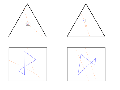
Figure 3. Periodic orbit whose projections to ${{\Sigma^{A}}}$ (left) and ${{\Sigma^{B}}}$ (right) are contained in convex cones with apexes ${E^{A}}$ and ${E^{B}}$ respectively. The dashed lines indicate the indifference lines of the players. Their intersections are the projections of the Nash equilibrium, ${E^{A}}$ and ${E^{B}}$. For better visibility, the bottom row shows a zoomed version of the periodic orbit.

Figure 4. Payoff along 10 periods of the periodic orbit contained in $P_{B}^{-}\times P_{A}^{-}$. Player A’s payoff oscillates around $-0.5$, player B’s payoff around $-0.25$. Nash equilibrium payoff is zero to both players.

This example has been obtained through numerical experimentation. The difficulty in finding an example of a periodic orbit with the key property of lying in a convex cone with apex at the unique, completely mixed Nash equilibrium seems to suggest that such examples are relatively rare. For most games with unique, completely mixed Nash equilibrium, payoff along typical FP orbits either Pareto dominates Nash equilibrium payoff or at least improves upon it along parts of the orbit. We formulate the following two conjectures.

Conjecture 5.3.

Bimatrix games with unique, completely mixed Nash equilibrium, where Nash equilibrium Pareto dominates typical FP orbits are rare. To be precise, within the space of $n\times n$ games with entries in $[0,1]$, those where typical FP orbits are Pareto dominated by Nash equilibrium form a set with at most Lebesgue measure $0.01$.

Conjecture 5.4.

For bimatrix games with unique, completely mixed Nash equilibrium and certain transition combinatorics (see [25]), Nash equilibrium does not Pareto dominate typical FP orbits. In particular, this is the case if ${{\mathcal{B}\!\mathcal{R}\!}_{A}}(e_{j})\neq{{\mathcal{B}\!\mathcal{R}\!}_{A}}(e_{j^{\prime}})$ for all $j\neq j^{\prime}$ and ${{\mathcal{B}\!\mathcal{R}\!}_{B}}(e_{i})\neq{{\mathcal{B}\!\mathcal{R}\!}_{B}}(e_{i^{\prime}})$ for all $i\neq i^{\prime}$.

Indeed, we could strengthen the above conjecture to the following statement.

Conjecture 5.5.

For ‘most’ bimatrix games with unique, completely mixed Nash equilibrium, typical FP orbits dominate Nash equilibrium in terms of average payoff. In particular, this is the case under certain assumptions on the transition combinatorics of the game; for instance, if each pure strategy invokes a distinct pure best response (as in the previous conjecture).

6. Concluding remarks on FP performance

Conceptually, the overall observation is that playing Nash equilibrium might not be an advantage over playing according to some learning algorithm (such as FP) in a wide range of games, in particular in many common examples of games occurring in the literature. Even in cases where FP does not dominate Nash equilibrium at all times, it might still be preferable in terms of time-averaged payoff. In contrast, the previous section shows that there are examples in which Nash equilibrium indeed Pareto dominates FP, but the restrictive nature of the example suggests that this situation is quite rare.

Conversely, the discussion also shows that certain notions of game equivalence (for instance, linear equivalence, or the weaker best and better response equivalences, see [23, 24]), which are popular in the literature on learning dynamics, are not meaningful in an economic context as they do not preserve essential features of the payoff structure of games, even though they preserve Nash equilibria (and other notions of equilibrium) and conditional preferences of the players. While some dynamics (in particular, FP dynamics or its autonomous version, the best response dynamics [13, 21, 19]) are invariant under all of these equivalence relations, the actual payoffs along their orbits and the payoff comparison of different orbits can strongly depend on the chosen representative bimatrix, as becomes apparent from Theorem 3.3. This is to some extent analogous to the situation in the classical example of the ‘prisoner’s dilemma’ given by the bimatrix

$$A=\begin{pmatrix}3&0\\ 5&1\end{pmatrix},\quad B=\begin{pmatrix}3&5\\ 0&1\end{pmatrix}.$$

Under linear equivalence, this corresponds to the bimatrix game

$$\tilde{A}=\begin{pmatrix}0&0\\ 2&1\end{pmatrix},\quad\tilde{B}=\begin{pmatrix}0&2\\ 0&1\end{pmatrix},$$

which shares all essential features such as equilibria, best response structures, etc with the prisoner’s dilemma. Both games are dynamically identical, with all FP orbits converging along straight lines to the unique pure Nash equilibrium $(2,2)$. However, the second game does not constitute a prisoner’s dilemma in the classical sense: whereas in the prisoner’s dilemma the Nash equilibrium is Pareto dominated by the (dynamically irrelevant) strategy profile $(1,1)$, in the second game this is not the case and no ‘dilemma’ occurs.

Theorem 3.3 can be interpreted in a similar vain: linear equivalence turns out to be sufficiently coarse, so that by changing the representative bimatrix inside an equivalence class, one can create certain regions in $\Sigma$ in which payoff is arbitrarily high in comparison to the payoff at the unique Nash equilibrium. Since FP orbits remain unchanged, this can be done in such a way that a given periodic orbit lies completely or predominantly in these desired ‘high payoff portions’ of $\Sigma$. On the other hand, it can be seen from the proof that the conditions for this to happen are not at all exceptional. Consequently, it could be argued that in many games of interest the assumption that Nash equilibrium play is the most desirable outcome might not hold and a more dynamic view of ‘optimal play’ might be reasonable.

References

- [1] R. J. Aumann. Subjectivity and correlation in randomized strategies. J. Math. Econom., 1:67–96, 1974.
- [2] R. J. Aumann. Correlated equilibrium as an expression of Bayesian rationality. Econometrica, 55(1):1–18, 1987.
- [3] U. Berger. Fictitious play in games. J. Econ. Theory, 120(2):139–154, 2005.
- [4] U. Berger. Two more classes of games with the continuous-time fictitious play property. Game. Econ. Behav., 60(2):247–261, 2007.
- [5] U. Berger. Learning in games with strategic complementarities revisited. J. Econ. Theory, 143(1):292–301, 2008.
- [6] D. Blackwell. Controlled random walks. In Proceedings of the International Congress of Mathematicians, volume 3, pages 336–338, 1954.
- [7] G. W. Brown. Some notes on computation of games solutions. Technical report, Report P-78, The Rand Corporation, 1949.
- [8] G. W. Brown. Iterative solution of games by fictitious play. In Activity Analysis of Production and Allocation, volume 13, pages 374–376. John Wiley & Sons, New York, 1951.
- [9] D. P. Foster and R. V. Vohra. Calibrated learning and correlated equilibrium. Game. Econ. Behav., 21(1-2):40–55, 1997.
- [10] D. Fudenberg and D. K. Levine. Consistency and cautious fictitious play. J. Econ. Dyn. Control, 19(5-7):1065–1089, 1995.
- [11] D. Fudenberg and D. K. Levine. The Theory of Learning in Games. MIT Press Series on Economic Learning and Social Evolution, 2. MIT Press, Cambridge, MA, 1998.
- [12] A. Gaunersdorfer and J. Hofbauer. Fictitious play, Shapley polygons, and the replicator equation. Game. Econ. Behav., 11(2):279–303, 1995.
- [13] I. Gilboa and A. Matsui. Social stability and equilibrium. Econometrica, 59(3):859–867, 1991.
- [14] J. Hannan. Approximation to Bayes risk in repeated play. Contributions to the Theory of Games, 3:97–139, 1957.
- [15] C. Harris. On the rate of convergence of continuous-time fictitious play. Game. Econ. Behav., 22(2):238–259, 1998.
- [16] S. Hart. Adaptive heuristics. Econometrica, 73(5):1401–1430, 2005.
- [17] S. Hart and A. Mas-Colell. A simple adaptive procedure leading to correlated equilibrium. Econometrica, 68(5):1127–1150, 2000.
- [18] S. Hart and A. Mas-Colell. A general class of adaptive strategies. J. Econ. Theory, 98(1):26–54, 2001.
- [19] J. Hofbauer. Stability for the best response dynamics. Mimeo, 1995.
- [20] V. Krishna and T. Sjöström. On the convergence of fictitious play. Math. Oper. Res., 23(2):479 – 511, 1998.
- [21] A. Matsui. Best response dynamics and socially stable strategies. J. Econ. Theory, 57(2):343–362, 1992.
- [22] D. Monderer, D. Samet, and A. Sela. Belief affirming in learning processes. J. Econ. Theory, 73(2):438–452, 1997.
- [23] S. Morris and T. Ui. Best response equivalence. Game. Econ. Behav., 49(2):260–287, 2004.
- [24] H. J. Moulin and J.-P. Vial. Strategically zero-sum games: the class of games whose completely mixed equilibria cannot be improved upon. Internat. J. Game Theory, 7(3-4):201–221, 1978.
- [25] G. Ostrovski and S. van Strien. Piecewise linear Hamiltonian flows associated to zero-sum games: transition combinatorics and questions on ergodicity. Regul. Chaotic Dyn., 16(1-2):129–154, 2011.
- [26] J. Rosenmüller. Über Periodizitätseigenschaften spieltheoretischer Lernprozesse. Z. Wahrscheinlichkeit., 17(4):259–308, 1971.
- [27] L. S. Shapley. Some topics in two-person games. Advances in Game Theory, 52:1–29, 1964.
- [28] C. Sparrow, S. van Strien, and C. Harris. Fictitious play in games: the transition between periodic and chaotic behaviour. Game. Econ. Behav., 63(1):259–291, 2008.
- [29] K. Sydsaeter and P. Hammond. Essential Mathematics for Economic Analysis. Prentice Hall, 3rd edition, 2008.
- [30] S. van Strien and C. Sparrow. Fictitious play in games: chaos and dithering behaviour. Game. Econ. Behav., 73(1):262–286, 2011.
- [31] H. P. Young. Strategic Learning and Its Limits (Arne Ryde Memorial Lectures Series). Oxford University Press, USA, 2005.