An Algorithm for the T-count

Abstract.

We consider quantum circuits composed of Clifford and $T$ gates. In this context the $T$ gate has a special status since it confers universal computation when added to the (classically simulable) Clifford gates. However it can be very expensive to implement fault-tolerantly. We therefore view this gate as a resource which should be used only when necessary. Given an $n$-qubit unitary $U$ we are interested in computing a circuit that implements it using the minimum possible number of $T$ gates (called the $T$-count of $U$). A related task is to decide if the $T$-count of $U$ is less than or equal to $m$; we consider this problem as a function of $N=2^{n}$ and $m$. We provide a classical algorithm which solves it using time and space both upper bounded as $\mathcal{O}(N^{m}\text{poly}(m,N))$. We implemented our algorithm and used it to show that any Clifford+T circuit for the Toffoli or the Fredkin gate requires at least 7 $T$ gates. This implies that the known 7 $T$ gate circuits for these gates are $T$-optimal. We also provide a simple expression for the $T$-count of single-qubit unitaries.

1. Introduction

The single-qubit $T$ gate

$$T=\left(\begin{array}[]{cc}1&0\\ 0&e^{i\frac{\pi}{4}}\end{array}\right),$$

along with all gates from the Clifford group, is a universal gate set for quantum computation. The $T$ gate is essential because circuits composed of only Clifford gates are classically simulable [6]. The $T$ gate also plays a special role in fault-tolerant quantum computation. In contrast with Clifford gates, the $T$ gate is not transversal for many quantum error-correcting codes, which means that in practice it is very costly to implement fault-tolerantly. For this reason we are interested in circuits which use as few $T$ gates as possible to implement a given unitary.

We consider unitaries which can be implemented exactly using Clifford and T gates. The set of all such unitaries is known: it was conjectured in [9] and later proven in [5] that an $n$-qubit unitary can be implemented using this gate set if and only if its matrix elements are in the ring $\mathbb{Z}\left[i,\frac{1}{\sqrt{2}}\right]$. In general this implementation requires one ancilla qubit prepared in the state $|0\rangle$ in addition to the $n$ qubits on which the computation is to be performed. An algorithm for exactly synthesizing unitaries over the gate set $\{H,T,\text{CNOT}\}$ was given in reference [5], and a superexponentially faster version of this algorithm was presented in reference [8].

In this paper we focus on the set of unitaries implementable without ancillas, that is to say, the group $\mathcal{J}_{n}$ generated by the $n$-qubit Clifford group and the T gate. An $n$-qubit unitary is an element of this group if and only if its matrix elements are in the ring $\mathbb{Z}\left[i,\frac{1}{\sqrt{2}}\right]$ and its determinant satisfies a simple condition [5] (when $n\geq 4$ the condition is that the determinant is equal to $1$). Notable examples include the Toffoli and Fredkin gates which are in the group $\mathcal{J}_{3}$.

For $U\in\mathcal{J}_{n}$, the $T$-count of $U$ is defined to be the minimum number of $T$ gates in a Clifford+T circuit that implements it (up to a possible global phase), and is denoted by $\mathcal{T}(U)$. In other words $\mathcal{T}(U)$ is the minimum $m$ for which

(1.1) $$e^{i\phi}U=C_{m}T_{(q_{m})}C_{m-1}T_{(q_{m-1})}\ldots T_{(q_{1})}C_{0}$$

where $\phi\in[0,2\pi)$, $C_{i}$ are in the $n$-qubit Clifford group, $q_{j}\in\{1,\ldots,n\}$, and $T_{(r)}$ indicates the $T$ gate acting on the $r$th qubit.

Note that it may be possible to implement some unitary using less than $\mathcal{T}(U)$ $T$ gates if one uses ancilla qubits and/or measurements with classically controlled operations. For example, Jones has shown how to perform a Toffoli gate using these additional ingredients and only four $T$ gates [7]. This does not contradict our result that $\mathcal{T}(\text{Toffoli)=7}$.

We are interested in the following problem. Given $U\in\mathcal{J}_{n}$, compute a $T$-optimal $n$-qubit quantum circuit for it, that is to say, a circuit which implements it (up to a global phase) using $\mathcal{T}(U)$ $T$ gates. A related, potentially easier problem, is to compute $\mathcal{T}(U)$ given $U$. It turns out that this latter problem is not much easier: we show in Section 3 that an algorithm which computes $\mathcal{T}(U)$ can be converted into an algorithm which outputs a T-optimal circuit for $U$, with overhead polynomial in $\mathcal{T}(U)$ and the dimension of $U$. For this reason, and for the sake of simplicity, we focus on the task of computing $\mathcal{T}(U)$.

Problem 1 (COUNT-T).

Given $U\in\mathcal{J}_{n}$ and $m\in\mathbb{N}$, decide if $\mathcal{T}(U)\leq m$.

We consider the complexity of this problem as a function of $m$ and $N=2^{n}$. We treat arithmetic operations on the entries of $U$ at unit cost, and we do not account for the bit-complexity associated with specifying or manipulating them. We present an algorithm which solves COUNT-T using time and space both upper bounded as $\mathcal{O}\left(N^{m}\text{poly}(m,N)\right)$. Our algorithm uses the meet-in-the-middle idea from [3] along with a representation for Clifford+T unitaries where the $T$ gates have a special role. We implemented our algorithm in C++ and used it to prove that the $T$-count of Toffoli and Fredkin gates is $7$. We also provide a simple expression for the $T$-count of single-qubit unitaries.

The problem of computing $T$-optimal circuits was studied in references [9, 3, 2]. In reference [9] an algorithm was given for synthesizing single-qubit circuits over the gate set $\{H,T\}$, and it was shown that the resulting circuits are $T$-optimal. The problem of reducing the number of $T$-gates in circuits with $n>1$ qubits was considered as an application of the meet-in-the-middle algorithm from reference [3], where some small examples of $T$-depth optimal circuits were found. The algorithm for optimizing $T$-depth presented in reference [3] can be used (with a small modification) to solve COUNT-T but its time complexity is $\Omega\left(2^{n^{2}\left\lfloor m/2\right\rfloor}\right)$ since the size of the $n$-qubit Clifford group is $\Omega\left(2^{n^{2}}\right)$[4]. It was conjectured in reference [3] that Toffoli requires 7 $T$ gates; we prove this conjecture in this paper. In reference [2] an algorithm based on matroid partitioning is given which can be used as a heuristic for minimizing the $T$-count and $T$-depth of quantum circuits. The algorithm we present here solves COUNT-T using time $\mathcal{O}\left(2^{nm}\text{poly}\left(m,2^{n}\right)\right)$, which is a superexponential speedup (as a function of $n$) over reference [3], and in contrast with the heuristic from [2] it computes the $T$-count exactly.

Our work, and previous work on the $T$-count, takes a different but complementary perspective from that of the recent paper [10]. That paper considers quantum states (e.g., magic states) as a resource for computation using Clifford circuits, and attempts to quantify the amount of resource in a given state. Here we view the $T$ gate as a resource and ask how much is necessary to implement a given unitary.

The rest of the paper is structured as follows. We begin in Section 2 by discussing the central objects that we study: Pauli and Clifford operators, and the group $\mathcal{J}_{n}$ generated by Clifford and $T$ gates. In Section 3 we give a decomposition for unitaries from the group $\mathcal{J}_{n}$. Using this decomposition we show how an algorithm for the $T$-count can be used to generate $T$-optimal circuits. In Section 4 we give a simple characterization of the $T$-count for single-qubit unitaries, and in Section 5 we present our algorithm for COUNT-T. We conclude in Section 6 with a discussion of open problems.

2. Preliminaries

In this Section we establish notation and we review facts about the Clifford+T gate set. Throughout this paper we write $N=2^{n}$ and $[K]=\{1,\ldots,K\}$. We write

$$X=\left(\begin{array}[]{cc}0&1\\ 1&0\end{array}\right)\qquad Y=\left(\begin{array}[]{cc}0&-i\\ i&0\end{array}\right)\qquad Z=\left(\begin{array}[]{cc}1&0\\ 0&-1\end{array}\right)$$

for the single-qubit Pauli matrices. We use a parenthesized subscript to indicate qubits on which an operator acts, e.g., $X_{(1)}=X\otimes\mathbb{I}^{\otimes\left(n-1\right)}$ indicates the Pauli $X$ matrix acting on the first qubit.

2.1. Cliffords and Paulis

The single-qubit Clifford group $\mathcal{C}_{1}$ is generated by the Hadamard and phase gates

$$\mathcal{C}_{1}=\left\langle H,T^{2}\right\rangle$$

where

$$H=\frac{1}{\sqrt{2}}\left(\begin{array}[]{cc}1&1\\ 1&-1\end{array}\right)\quad T^{2}=\left(\begin{array}[]{cc}1&0\\ 0&i\end{array}\right).$$

When $n>1$, the $n$-qubit Clifford group $\mathcal{C}_{n}$ is generated by these two gates (acting on any of the $n$ qubits) along with the two-qubit $\text{CNOT}=|0\rangle\langle 0|\otimes\mathbb{I}+|1\rangle\langle 1|\otimes X$ gate (acting on any pair of qubits). The Clifford group is special because of its relationship to the set of $n$-qubit Pauli operators

$$\mathcal{P}_{n}=\left\{Q_{1}\otimes Q_{2}\otimes\ldots\otimes Q_{n}:\;Q_{i}\in\{\mathbb{I},X,Y,Z\}\right\}.$$

Cliffords map Paulis to Paulis, up to a possible phase of $-1$, i.e., for any $P\in\mathcal{P}_{n}$ and any $C\in\mathcal{C}_{n}$ we have

$$CPC^{\dagger}=(-1)^{b}P^{\prime}$$

for some $b\in\{0,1\}$ and $P^{\prime}\in\mathcal{P}_{n}$. It is easy to prove that, given two Paulis, neither equal to the identity, it is always possible to (efficiently) find a Clifford which maps one to the other. For completeness we include a proof in the Appendix.

Fact 1.

For any $P,P^{\prime}\in\mathcal{P}_{n}\setminus\{\mathbb{I}\}$ there exists a Clifford $C\in\mathcal{C}_{n}$ such that $CPC^{\dagger}=P^{\prime}$. A circuit for $C$ over the gate set $\{H,T^{2},\text{CNOT}\}$ can be computed efficiently (as a function of $n$).

2.2. The group $\mathcal{J}_{n}$ generated by Clifford and T gates

We consider the group $\mathcal{J}_{n}$ generated by the $n$-qubit Clifford group along with the $T$ gate. For a single qubit

$$\mathcal{J}_{1}=\left\langle H,T\right\rangle,$$

and for $n>1$ qubits

$$\mathcal{J}_{n}=\left\langle H_{(i)},T_{(i)},\text{CNOT}_{(i,j)}:\;i,j\in[n]\right\rangle$$

(recall the subscript indicates qubits on which the gate acts). It is not hard to see that $\mathcal{J}_{n}$ is a group, since the Hadamard and CNOT gates are their own inverses and $T^{-1}=T^{7}$.

Noting that $H,T,$ and CNOT all have matrix elements over the ring

$$\mathbb{Z}\left[i,\frac{1}{\sqrt{2}}\right]=\left\{\frac{a+bi+c\sqrt{2}+di\sqrt{2}}{\sqrt{2}^{k}}:\;a,b,c,d\in\mathbb{Z},\;k\in\mathbb{N}\right\},$$

we see that any $U\in\mathcal{J}_{n}$ also has matrix elements from this ring. Giles and Selinger [5] proved that this condition, along with a simple condition on the determinant, exactly characterizes $\mathcal{J}_{n}$.

Theorem (Corollary 2 from [5]).

$$\mathcal{J}_{n}=\left\{U\in U(N):\>\text{Each entry of $U$is an element of }\mathbb{Z}\left[i,\frac{1}{\sqrt{2}}\right],\text{ and }\det U=e^{i\frac{\pi}{8}Nr}\text{ for some }r\in[8]\right\}$$

where $N=2^{n}.$

Note that for $n\geq 4$ the condition on the determinant is simply $\det U=1$.

2.3. Channel representation, and modding out global phases

Consider the action of an $n$-qubit unitary $U$ on a Pauli $P_{s}\in\mathcal{P}_{n}$

(2.1) $$UP_{s}U^{\dagger}.$$

The set of all such operators (with $P_{s}\in\mathcal{P}_{n}$) completely determines $U$ up to a global phase. Since $\mathcal{P}_{n}$ is a basis for the space of all Hermitian $N\times N$ matrices, we can expand (2.1) as

(2.2) $$UP_{s}U^{\dagger}=\sum_{P_{r}\in\mathcal{P}_{n}}\widehat{U}_{rs}P_{r},$$

where

(2.3) $$\widehat{U}_{rs}=\frac{1}{2^{n}}\text{Tr}\left(P_{r}UP_{s}U^{\dagger}\right).$$

This defines a $N^{2}\times N^{2}$ matrix $\widehat{U}$ with rows and columns indexed by Paulis $P_{r},P_{s}\in\mathcal{P}_{n}$. We refer to $\widehat{U}$ as the channel representation of $U$.

By Hermitian-conjugating (2.2) we see that each matrix element of $\widehat{U}$ is real. It is also straightforward to check, using (2.2), that the channel representation respects matrix multiplication:

$$\widehat{UV}=\widehat{U}\widehat{V}.$$

Setting $V=U^{\dagger}$ and using the fact that $\widehat{U^{\dagger}}=\left(\widehat{U}\right)^{\dagger}$, we see that the channel representation $\widehat{U}$ is unitary.

In this paper we use the channel representation for $U\in\mathcal{J}_{n}$. In this case, the entries of $U$ are in the ring $\mathbb{Z}\left[i,\frac{1}{\sqrt{2}}\right]$, and from (2.3) we see that so are the entries of $\widehat{U}$. Since $\widehat{U}$ is also real, its entries are from the subring

$$\mathbb{Z}\left[\frac{1}{\sqrt{2}}\right]=\left\{\frac{a+b\sqrt{2}}{\sqrt{2}^{k}}:\;a,b\in\mathbb{Z},\;k\in\mathbb{N}\right\}.$$

The channel representation identifies unitaries which differ by a global phase. We write

$$\widehat{\mathcal{J}_{n}} =\left\{\widehat{U}:\;U\in\mathcal{J}_{n}\right\},\qquad\widehat{\mathcal{C}_{n}}=\left\{\widehat{C}:\;C\in\mathcal{C}_{n}\right\}$$

for the groups in which global phases are modded out. Note that each $Q\in\widehat{\mathcal{C}_{n}}$ is a unitary matrix with one nonzero entry in each row and each column, equal to $\pm 1$ (since Cliffords map Paulis to Paulis up to a possible phase of $-1$). The converse also holds: if $W\in\widehat{\mathcal{J}_{n}}$ has this property then $W\in\widehat{\mathcal{C}_{n}}$.

Finally, note that since the definition of $T$-count is insensitive to global phases, it is well-defined in the channel representation; for $U\in\mathcal{J}_{n}$ we define $\mathcal{T}(\widehat{U})=\mathcal{T}(U)$.

3. decomposition for unitaries in $\mathcal{J}_{n}$

In this Section we present a decomposition for unitaries over the Clifford+$T$ gate set and we use it to show that an algorithm for COUNT-T can be used to generate a $T$-optimal circuit for $U\in\mathcal{J}_{n}$ with overhead polynomial in $\mathcal{T}(U)$ and $N$.

By definition, any $U\in\mathcal{J}_{n}$ can be written as an alternating product of Cliffords and T gates as in equation (1.1). The number $m$ of $T$ gates in (1.1) can be taken to be $\mathcal{T}(U)$, and we can reorganize it so that each $T$ gate is conjugated by a Clifford:

(3.1) $$U=e^{i\phi}\left(\prod_{i=\mathcal{T}(U)}^{1}D_{i}T_{(q_{i})}D_{i}^{\dagger}\right)D_{0}$$

where $D_{i}=\prod_{j=\mathcal{T}(U)}^{i}C_{j}$ for $i\in\{0,1,\ldots,\mathcal{T}(U)\}$. Note that

$$D_{i}T_{(q_{i})}D_{i}^{\dagger}=\frac{1}{2}\left(1+e^{i\frac{\pi}{4}}\right)\mathbb{I}+\frac{1}{2}\left(1-e^{i\frac{\pi}{4}}\right)D_{i}Z_{(q_{i})}D_{i}^{\dagger}.$$

In the second term we have a Pauli operator conjugated by a Clifford, which is equal to another Pauli (up to a possible phase of $-1$). In other words (3.1) can be written

(3.2) $$U=e^{i\phi}\left(\prod_{i=\mathcal{T}(U)}^{1}R((-1)^{b_{i}}P_{i})\right)D_{0}$$

where $P_{i}\in\mathcal{P}_{n}\setminus\{\mathbb{I}\}$ , $b_{i}\in\{0,1\}$, and

$$R(\pm P)=e^{i\frac{\pi}{8}\left(\mathbb{I}\mp P\right)}=\frac{1}{2}\left(1+e^{i\frac{\pi}{4}}\right)\mathbb{I}\pm\frac{1}{2}\left(1-e^{i\frac{\pi}{4}}\right)P\qquad P\in\mathcal{P}_{n}\setminus\{\mathbb{I}\}.$$

The following Proposition shows that such a decomposition exists with $b_{i}=0$ for all $i\in[\mathcal{T}(U)]$.

Proposition 1.

For any $U\in\mathcal{J}_{n}$ there exists a phase $\phi\in[0,2\pi),$ a Clifford $C_{0}\in\mathcal{C}_{n}$ and Paulis $P_{i}\in\mathcal{P}_{n}\setminus\{\mathbb{I}\}$ for $i\in[\mathcal{T}(U)]$ such that

(3.3) $$U=e^{i\phi}\left(\prod_{i=\mathcal{T}(U)}^{1}R(P_{i})\right)C_{0}.$$

Proof.

For any $Q\in\mathcal{P}_{n}\setminus\{\mathbb{I}\}$ we have

(3.4) $$R(-Q)=e^{i\frac{\pi}{8}\left(1+Q\right)}=R(Q)e^{i\frac{\pi}{4}Q}.$$

Note, using Fact 1, that $e^{i\frac{\pi}{4}Q}=Ce^{i\frac{\pi}{4}Z_{(1)}}C^{\dagger}$ for some $C\in\mathcal{C}_{n}$, and

$$e^{i\frac{\pi}{4}Z_{(1)}}=e^{i\frac{\pi}{4}}\left(T_{(1)}\right)^{6}.$$

Now using the fact that $T^{6}$ is Clifford we get $e^{-i\frac{\pi}{4}}e^{i\frac{\pi}{4}Q}\in\mathcal{C}_{n}$.

By repeatedly using (3.4) we transform (3.2) into the form (3.3) (with a potentially different set of Paulis $P_{i}$). Start with the decomposition (3.2) and let $j\in[\mathcal{T}(U)]$ be the largest index such that $b_{j}=1$. Then

$$U =e^{i\phi}\left(\prod_{i=\mathcal{T}(U)}^{j+1}R\left(P_{i}\right)\right)R(-P_{j})\left(\prod_{i=j-1}^{1}R\left((-1)^{b_{i}}P_{i}\right)\right)D_{0}$$

$$=e^{i\phi}\left(\prod_{i=\mathcal{T}(U)}^{j+1}R\left(P_{i}\right)\right)R(P_{j})e^{i\frac{\pi}{4}P_{j}}\left(\prod_{i=j-1}^{1}R\left((-1)^{b_{i}}P_{i}\right)\right)D_{0}$$

(3.5) $$=e^{i\left(\phi+\frac{\pi}{4}\right)}\left(\prod_{i=\mathcal{T}(U)}^{j}R\left(P_{i}\right)\right)\left[e^{-i\frac{\pi}{4}}e^{i\frac{\pi}{4}P_{j}}\left(\prod_{i=j-1}^{1}R\left((-1)^{b_{i}}P_{i}\right)\right)D_{0}\right].$$

Note that all the Paulis outside of the square brackets have $+$ signs in front of them. The unitary in square brackets has $T$-count $j-1$ (since $e^{-i\frac{\pi}{4}}e^{i\frac{\pi}{4}P_{j}}\in\mathcal{C}_{n}$) and can therefore be written as in equation (3.2) with $j-1$ terms in the product. We now recurse, applying the above steps to this unitary in square brackets. We repeat this procedure (at most $j-1$ more times) until all the minus signs are replaced with plus signs. ∎

Remark.

The channel representation $\widehat{U}$ inherits the decomposition from Proposition 1, and in this representation the global phase goes away, i.e.,

(3.6) $$\widehat{U}=\left(\prod_{i=\mathcal{T}(U)}^{1}\widehat{R(P_{i})}\right)\widehat{C_{0}}.$$

Computing $T$-optimal circuits using an algorithm for COUNT-T

Suppose that we have an algorithm $\mathcal{A}$ which solves the decision problem COUNT-T. For any $U\in\mathcal{J}_{n}$, we show that, with overhead polynomial in $N$ and $\mathcal{T}(U)$, such an algorithm can also be used to generate a $T$-optimal circuit for $U$ over the gate set $\{H,T,CNOT\}$. This is a simple application of the decomposition (3.3).

First note that $\mathcal{A}$ can be used to compute $\mathcal{T}(U)$, by starting with $m=0$ and running $\mathcal{A}$ on each nonnegative integer in sequence until we find $m-1$ and $m$ with $\mathcal{T}(U)\leq m$ and $\mathcal{T}(U)>m-1$. In this way we first compute $\mathcal{T}(U)$ and then we try each Pauli $Q\in\mathcal{P}_{n}\setminus\{\mathbb{I}\}$ until we find one which satisfies

$$\mathcal{T}\left(R(Q)^{\dagger}U\right)=\mathcal{T}(U)-1.$$

Note that (3.3) implies that at least one such Pauli $Q$ exists. Repeating this procedure $\mathcal{T}(U)-1$ more times we get Paulis $Q_{1},\ldots,Q_{\mathcal{T}(U)}$ such that

$$\mathcal{T}\left(R(Q_{1})^{\dagger}\ldots R(Q_{\mathcal{T}(U)-1})^{\dagger}R(Q_{\mathcal{T}(U)})^{\dagger}U\right)=0.$$

In other words

(3.7) $$e^{i\phi}U=R(Q_{\mathcal{T}(U)})R(Q_{\mathcal{T}(U)-1})\ldots R(Q_{1})C_{0}$$

where $\phi\in[0,2\pi)$ and $C_{0}\in\mathcal{C}_{n}$.

The next step is to compute a circuit which implements $C_{0}$ up to a global phase. To this end, we compute the channel representation $\widehat{C_{0}}$ explicitly as an $N^{2}\times N^{2}$ matrix using the fact that

$$\widehat{C_{0}}=\widehat{R(Q_{1})^{\dagger}}\ldots\widehat{R(Q_{\mathcal{T}(U)-1})^{\dagger}}\widehat{R(Q_{\mathcal{T}(U)})^{\dagger}}\widehat{U}.$$

We then use standard techniques to obtain a circuit which implements $C_{0}$ (up to a global phase) over the gate set $\{H,T^{2},\text{CNOT}\}$. For example, this can be done efficiently using the procedure outlined in the proof of Theorem 8 from reference [1].

Now using Fact 1 there are Cliffords $C_{1},\ldots,C_{\mathcal{T}(U)}\in\mathcal{C}_{n}$ which map each of the Paulis $Q_{1},\ldots,Q_{\mathcal{T}(U)}$ to $Z$ acting on the first qubit, i.e.,

$$C_{i}Q_{i}C_{i}^{\dagger}=Z_{(1)}$$

for each $i\in[\mathcal{T}(U)]$, and we can efficiently compute circuits for each of these Cliffords. Using the fact that $R(Z_{(1)})=T_{(1)}$ and plugging into equation (3.7) gives

$$e^{i\phi}U=\left(\prod_{j=\mathcal{T}(U)}^{1}C_{j}^{\dagger}T_{(1)}C_{j}\right)C_{0}.$$

The RHS, along with the circuits for $C_{0},\ldots,C_{\mathcal{T}(U)}$ discussed above, gives a $T$-optimal implementation of $U$ (up to a global phase) over the gate set $\{H,T,\text{CNOT\}}$.

4. $T$-count for single-qubit unitaries

In this Section we show how the $T$-count of a single-qubit unitary $U\in\mathcal{J}_{1}$ can be directly computed from its channel representation $\widehat{U}$.

Recall that $\widehat{U}$ has entries over the ring $\mathbb{Z}\left[\frac{1}{\sqrt{2}}\right]$. For any nonzero element $\frac{a+b\sqrt{2}}{\sqrt{2}^{k}}$ of this ring, the integer $k$ can be chosen to be minimal in the following sense. If $a$ is even and $k>0$ then we can divide the top and bottom by $\sqrt{2}$ and reduce $k$ by one. When $a$ is odd or $k=0$, $k$ cannot be reduced any further, and we call it the smallest denominator exponent. Similar quantities were defined in references [9] and [5].

Definition 1.

For any nonzero $v\in\mathbb{\mathbb{Z}}\left[\frac{1}{\sqrt{2}}\right]$ the smallest denominator exponent, denoted by $\text{sde}(v)$, is the smallest $k\in\mathbb{N}$ for which

$$v=\frac{a+b\sqrt{2}}{\sqrt{2}^{k}}$$

with $a,b\in\mathbb{Z}$. We define $\mathrm{sde}(0)=0$. For a $d_{1}\times d_{2}$ matrix $M$ with entries over this ring we define

$$\mathrm{sde}\left(M\right)=\max_{a\in[d_{1}],b\in[d_{2}]}\mathrm{sde}(M_{ab}).$$

We use the following fact which is straightforward to prove.

Fact 2.

Let $q,r\in\mathbb{\mathbb{Z}}\left[\frac{1}{\sqrt{2}}\right]$ with $\mathrm{sde}(q)>\mathrm{sde}(r)$. Then

$$\mathrm{sde}\left(\frac{1}{\sqrt{2}}\left(q\pm r\right)\right)=\mathrm{sde}(q)+1.$$

The $T$-count of a single qubit unitary is simply equal to the $\mathrm{sde}$ of its channel representation.

Theorem 1.

The $T$-count of a single-qubit unitary $U\in\mathcal{J}_{1}$ is

$$\mathcal{T}(U)=\mathrm{sde}(\widehat{U}).$$

Proof.

By Proposition 1, $U$ can be decomposed as (3.3), as a global phase times a product of $R(P_{i})$ operators times $C_{0}$, with $P_{i}\in\{X,Y,Z\}$ for all $i$ and $C_{0}\in\mathcal{C}_{1}$. Note $\mathcal{T}\left(U\right)=\mathcal{T}(UC_{0}^{\dagger})$ and

(4.1) $$\widehat{UC_{0}^{\dagger}}=\prod_{i=\mathcal{T}(U)}^{1}\widehat{R(P_{i})}.$$

The operators which appear on the RHS are

(4.2) $$\widehat{R(X)}=\left(\begin{array}[]{cccc}1&0&0&0\\ 0&1&0&0\\ 0&0&\frac{1}{\sqrt{2}}&-\frac{1}{\sqrt{2}}\\ 0&0&\frac{1}{\sqrt{2}}&\frac{1}{\sqrt{2}}\end{array}\right)\quad\widehat{R(Y)}=\left(\begin{array}[]{cccc}1&0&0&0\\ 0&\frac{1}{\sqrt{2}}&0&\frac{1}{\sqrt{2}}\\ 0&0&1&0\\ 0&-\frac{1}{\sqrt{2}}&0&\frac{1}{\sqrt{2}}\end{array}\right)\quad\widehat{R(Z)}=\left(\begin{array}[]{cccc}1&0&0&0\\ 0&\frac{1}{\sqrt{2}}&-\frac{1}{\sqrt{2}}&0\\ 0&\frac{1}{\sqrt{2}}&\frac{1}{\sqrt{2}}&0\\ 0&0&0&1\end{array}\right)$$

where the rows and columns are labeled by Paulis $\mathrm{\mathbb{I},X,Y,Z}$ from top to bottom and left to right. Note that

$$\widehat{R(X)}^{2}=\widehat{R(Y)}^{2}=\widehat{R(Z)}^{2}=\mathbb{I}.$$

Since (4.1) uses the minimal number of $T$ gates, we see that no two consecutive Paulis in this decomposition are equal, i.e., $P_{i}\neq P_{i+1}$ for all $i\in[\mathcal{T}(U)-1]$.

Consider the entries of (4.1). Since it is a product of the matrices (4.2), we see that the top left entry is always $1$ and all other entries in the first row and column are $0$. We therefore focus on the lower-right $3\times 3$ submatrix. Looking at this submatrix for $\widehat{R(X)}$, $\widehat{R(Y)}$ and $\widehat{R(Z)}$ we see that there are two rows with $\mathrm{sde}$ equal to $1$ and one row where it is $0$ (recall from Definition 1 that the $\mathrm{sde}$ of a row vector is the maximum $\mathrm{sde}$ of one of its entries). The rows with $\mathrm{sde}$ $0$ in the lower-right $3\times 3$ submatrix of $\widehat{R(X)}$, $\widehat{R(Y)}$ and $\widehat{R(Z)}$ are labeled by $X$, $Y$ and $Z$ respectively. Taking this as the base case, we prove by induction that the lower right $3\times 3$ submatrix of (4.1) contains two rows with $\mathrm{sde}$ $\mathcal{T}(U)$ and one row with $\mathrm{sde}$ $\mathcal{T}(U)-1$, and this latter row is the one labeled by the Pauli $P_{\mathcal{T}(U)}$. We suppose this holds for $\mathcal{T}(U)=k$ and we show this implies it holds when $\mathcal{T}(U)=k+1$. When $\mathcal{T}(U)=k+1$ we consider

(4.3) $$M_{k+1}=\prod_{i=k+1}^{1}\widehat{R(P_{i})} =\widehat{R(P_{k+1})}M_{k}$$

where $M_{k}=\prod_{i=k}^{1}\widehat{R(P_{i})}$. Consider the lower-right $3\times 3$ submatrix of $M_{k}$. Using the inductive hypothesis, the row labeled $P_{k}$ has $\mathrm{sde}$ $k-1$, and the other two rows have $\mathrm{sde}$ $k$. Since $P_{k+1}\neq P_{k}$, one of these two rows is the one labeled $P_{k+1}$ and we write $Q=\{X,Y,Z\}\setminus\{P_{k},P_{k+1}\}$ for the other one. Note (looking at equation (4.2)) that left multiplying $M_{k}$ by $\widehat{R(P_{k+1})}$ leaves the row $P_{k+1}$ alone but replaces rows $P_{k}$ and $Q$ with $\frac{1}{\sqrt{2}}$ times their sum and difference (in some order). The row $P_{k+1}$ of $M_{k+1}$ therefore has $\mathrm{sde}$ equal to $k$, as required. Using the fact that row $P_{k}$ of $M_{k}$ has $\mathrm{sde}$ $k$ and row $Q$ of $M_{k}$ has $\mathrm{sde}$ $k-1,$ and using Fact 2, we see that the two row vectors obtained by taking $\frac{1}{\sqrt{2}}$ times their sum and difference both have $\mathrm{sde}$ $k+1$. Hence the two rows of $M_{k+1}$ labeled $P_{k}$ and $Q$ have $\mathrm{sde}$ $k+1$. This completes the proof. ∎

5. Algorithm for the T-count

In this Section we present an algorithm which solves COUNT-T using $\mathcal{O}\left(N^{m}\text{poly}(m,N)\right)$ time and space.

A naive approach would be to exhaustively search over products of the form (1.1) which alternate Clifford group elements and T gates, stopping if we find an expression equal to $e^{i\phi}U$. This does not work very well. Equation (1.1) has $m+1$ Clifford group elements and $m$ T-gates (each of which may act on any out of the $n$ qubits), so the number of products of this form is

$$|\mathcal{C}_{n}|^{m+1}n^{m}.$$

A better approach is use Proposition 1 and search over expressions of the form

(5.1) $$\left(\prod_{i=m}^{1}R(P_{i})\right)C_{0}$$

until we find one which is equal to $e^{i\phi}U$ for some phase $\phi$. In this case the size of the search space is $N^{2m}|\mathcal{C}_{n}|$ (recall $N=2^{n}$). However, a small modification improves this algorithm substantially. Rather than searching for expressions of the form (5.1) until we find one that is equal to $e^{i\phi}U$, we can search over expressions

$$U^{\dagger}\prod_{i=m}^{1}R(P_{i})$$

until we find one that is a global phase times an element of the Clifford group $\mathcal{C}_{n}$. This reduces the size of the search space to $N^{2m}$. The goal of the rest of this Section is to describe a more complicated algorithm which obtains (roughly) a square-root improvement at the expense of increasing the memory used.

We work in the channel representation, i.e., we consider the group $\widehat{\mathcal{J}_{n}}$. To describe our algorithm it will be convenient to have a notion of equivalence of unitaries up to right-multiplication by a Clifford. To be precise, we consider the left cosets of $\widehat{\mathcal{C}_{n}}$ in $\widehat{\mathcal{J}_{n}}$. We now show how to compute a (matrix-valued) function which tells you whether or not two unitaries $W,V\in\widehat{\mathcal{J}_{n}}$ are from the same coset, i.e., whether or not $W=VC$ for some $C\in\widehat{\mathcal{C}_{n}}.$

Definition 2 (Coset label).

Let $W\in\widehat{\mathcal{J}_{n}}$ . We define $W^{(c)}$ to be the matrix obtained from $W$ by the following procedure. First rewrite $W$ so that each nonzero entry has a common denominator, equal to $\sqrt{2}^{\mathrm{sde}(W)}$ (recall $\mathrm{sde}$ is defined for matrices in Definition 1). For each column of $W$, look at the first nonzero entry (from top to bottom) which we write as $v=\frac{a+b\sqrt{2}}{\sqrt{2}^{\mathrm{sde}(W)}}$. If $a<0$, or if $a=0$ and $b<0$, multiply every element of the column by $-1$. Otherwise, if $a>0$ or $a=0$ and $b>0$, do nothing and move on to the next column. After performing this step on all columns, permute the columns so they are ordered lexicographically from left to right.

The following Proposition shows that the function $W\rightarrow W^{(c)}$ labels cosets faithfully, so that two unitaries have the same label if and only if they are from the same coset.

Proposition 2.

Let $W,V\in\widehat{\mathcal{J}_{n}}$. Then $W^{(c)}=V^{(c)}$ if and only if $W=VC$ for some $C\in\widehat{\mathcal{C}_{n}}$.

Proof.

First suppose $W=VC$ with $C\in\widehat{\mathcal{C}_{n}}$. Since $C\in\widehat{\mathcal{C}_{n}}$ it has exactly one nonzero entry in every row and every column, equal to either $1$ or $-1$. In other words $W$ is obtained from $V$ by permuting columns and multiplying some of them by $-1$. Given this fact, we see from Definition 2 that $W^{(c)}=V^{(c)}$.

Now suppose $W^{(c)}=V^{(c)}$. From Definition 2 we see that $W^{(c)}=WD_{1}\pi_{1}$, where $D_{1}$ is diagonal and has diagonal entries all $\pm 1$, and $\pi_{1}$ is a permutation matrix. Likewise we can write $V^{(c)}=VD_{2}\pi_{2}$. Now setting these expressions equal we get

(5.2) $$W=VC,\quad\text{where}\quad C=D_{2}\pi_{2}\pi_{1}^{-1}D_{1}^{-1}.$$

Note that $C=V^{\dagger}W\in\widehat{\mathcal{J}_{n}}$. Since $C=D_{2}\pi_{2}\pi_{1}^{-1}D_{1}^{-1}$, we see that it has a single nonzero entry in each row and in each column, equal to either $+1$ or $-1$. Putting these two facts together we get $C\in\widehat{\mathcal{C}_{n}}$ (since any unitary in $\widehat{\mathcal{J}_{n}}$ with nonzero entries all $\pm 1$ is in $\widehat{\mathcal{C}_{n}}$). ∎

Our algorithm uses a sorted coset database, defined as follows.

Definition 3 (Sorted coset database $\mathcal{D}_{k}^{n}$).

For any $k\in\mathbb{N}$, a sorted coset database $\mathcal{D}_{k}^{n}$ is a list of unitaries $W\in\widehat{\mathcal{J}_{n}}$ with the following three properties:

1. Every unitary in the database has $T$-count $k$. Every $W\in\mathcal{D}_{k}^{n}$ satisfies $\mathcal{T}(W)=k$.

2. For any unitary with $T$-count $k$, there is a unique unitary in the database with the same coset label. For any $V\in\widehat{\mathcal{J}_{n}}$ with $\mathcal{T}(V)=k$, there exists a unique $W\in\mathcal{D}_{k}^{n}$ such that $W^{(c)}=V^{(c)}$.

3. The database is sorted according to the coset labels. If $W,V\in\mathcal{D}_{k}^{n}$ and $W^{(c)}<V^{(c)}$ (using lexicographic ordering on the matrices) then $W$ appears before $V$.

A sorted coset database can be viewed mathematically as a list of unitaries, but in practice when we implement such a database on a computer it makes sense to store each unitary along with its coset label as a pair $\left(W,W^{(c)}\right)$. This ensures that coset labels do not need to be computed on the fly during the course of our algorithm.

5.1. Algorithm

We are given as input a unitary $U\in\mathcal{J}_{n}$ and a nonnegative integer $m$. The algorithm determines if $\mathcal{T}(U)\leq m$, and if it is, also computes $\mathcal{T}(U)$.

1. Precompute sorted coset databases $\mathcal{D}_{0}^{n},\mathcal{D}_{1}^{n},\ldots,D_{\left\lceil\frac{m}{2}\right\rceil}^{n}$. To generate these databases, we start with $\mathcal{D}_{0}^{n}$ which contains only the $N^{2}\times N^{2}$ identity matrix. We then construct $\mathcal{D}_{1}^{n}$, then $\mathcal{D}_{2}^{n}$, up to $D_{\left\lceil\frac{m}{2}\right\rceil}^{n}$ as follows. To construct $\mathcal{D}_{k}^{n}$ we consider all unitaries of the form

   (5.3) $$W=R(P)M,$$

   where $M\in\mathcal{D}_{k-1}^{n}$ and $P\in\mathcal{P}_{n}\setminus\{\mathbb{I}\}$, one at a time. We insert $W$ into $\mathcal{D}_{k}^{n}$ (maintaining the ordering according to the coset labels) if and only if its coset label is new. That is to say, if and only if no unitary $V$ in one of the database $\mathcal{D}_{0}^{n},\mathcal{D}_{1}^{n},\ldots,D_{k-1}^{n}$ or in the partially constructed database $\mathcal{D}_{k}^{n}$ satisfies $W^{(c)}=V^{(c)}$.

2. Check if $\mathcal{T}(U)\leq\left\lceil\frac{m}{2}\right\rceil$. Use binary search to check if there exists $W\in\mathcal{D}_{j}^{n}$ for some $j\in\{0,1,...,\left\lceil\frac{m}{2}\right\rceil\}$, such that $\widehat{U}^{(c)}=W^{(c)}$. If so, output $\mathcal{T}(U)=j$ and stop. If not, proceed to step 3.

3. Meet-in-the-middle search. Start with $r=\left\lceil\frac{m}{2}\right\rceil+1$ and do the following. For each $W\in\mathcal{D}_{r-\left\lceil\frac{m}{2}\right\rceil}^{n}$, use binary search to find $V\in\mathcal{D}_{\left\lceil\frac{m}{2}\right\rceil}^{n}$ satisfying $\left(W^{\dagger}\widehat{U}\right)^{(c)}=V^{(c)}$, if it exists. If we find $W$ and $V$ satisfying this condition, we conclude $\mathcal{T}(U)=r$ and stop. If no such pair of unitaries is found, and if $r\leq m-1$, we increase $r$ by one and repeat this step; if $r=m$ we conclude $\mathcal{T}(U)>m$ and stop.

Let us now consider the time and memory resources required by this algorithm. First consider step $1$. To compute the sorted coset databases we loop over all unitaries of the form 5.3, with $k\in\{0,\ldots,\left\lceil\frac{m}{2}\right\rceil\}$. There are $\mathcal{O}\left(N^{2\left\lceil\frac{m}{2}\right\rceil}\right)$ such unitaries since $|\mathcal{P}_{n}|=N^{2}.$ For each unitary we need to compute the coset label and search to find it in databases generated so far; since the databases are sorted, the search can be done using $\mathcal{O}(\text{log}(N^{2\left\lceil\frac{m}{2}\right\rceil}))$ comparisons. The objects we are comparing (the unitaries and their coset labels) are themselves of size $N^{2}\times N^{2}$, so step 1. takes time $\mathcal{O}(N^{m}\text{poly}(m,N))$. To store the databases likewise requires space $\mathcal{O}(N^{m}\text{poly}(m,N))$. Step 2. takes time $\mathcal{O}(\text{poly}(m,N))$ since the binary search can be performed quickly. In step 3. we loop over all elements of the databases until we reach the stopping condition; the total time required in this step is $\mathcal{O}(N^{m}\text{poly}(m,N))$.

5.2. Correctness of the algorithm

To prove that the output of our algorithm is correct, we first show that step 1. of the algorithm correctly generates sorted coset databases $\mathcal{D}_{0}^{n},\mathcal{D}_{1}^{n},\ldots,D_{\left\lceil\frac{m}{2}\right\rceil}^{n}$. Given this fact, it is clear that if $0\leq\mathcal{T}(U)\leq\left\lceil\frac{m}{2}\right\rceil$ then step 2. of the algorithm will correctly compute $\mathcal{T}(U)$. In the following we show that if $\left\lceil\frac{m}{2}\right\rceil<\mathcal{T}(U)\leq m$ then step 3. computes it (and otherwise outputs $\mathcal{T}(U)>m$).

First consider step 1. It is not hard to see that $\mathcal{D}_{0}^{n}$, which contains only the identity matrix, is a sorted coset database (since all unitaries with $T$-count $0$ are Cliffords, and every Clifford has the same coset label as the identity matrix).

We now use induction; we assume that $\mathcal{D}_{0}^{n},\mathcal{D}_{1}^{n},\ldots,D_{k-1}^{n}$ are sorted coset databases and show this implies that $\mathcal{D}_{k}^{n}$, as generated by the algorithm, is a sorted coset database. We confirm properties (a), (b), and (c) from Definition 3. First suppose $W$ is added to the list $\mathcal{D}_{k}^{n}$ by the algorithm. This implies it has the form

(5.4) $$W=\prod_{i=k}^{1}\widehat{R(P_{i})}$$

for some $\{P_{i}\}\in\mathcal{P}_{n}\setminus\{\mathbb{I}\}$, and that its coset label is not equal to that of some other unitary $V\in\mathcal{D}_{j}^{n}$ with $j<k$. From (5.4) we see that $\mathcal{T}(W)\leq k$. Using the inductive hypothesis we see that $\mathcal{T}(W)>k-1$, since otherwise there would exist $V\in\mathcal{D}_{\mathcal{T}(W)}^{n}$ with $W^{(c)}=V^{(c)}$. Hence $\mathcal{T}(W)=k$ and $\mathcal{D}_{k}^{n}$ satisfies property (a). Now suppose that $Q\in\widehat{\mathcal{J}_{n}}$ has $\mathcal{T}(Q)=k$. Using the fact that $\mathcal{D}_{k-1}^{n}$ is a sorted coset database, there exists $M\in\mathcal{D}_{k-1}^{n}$ and $P\in\mathcal{P}_{n}\setminus\{\mathbb{I}\}$ such that $Q^{(c)}=\left(R(P)M\right)^{(c)}$. Now looking at the method by which $\mathcal{D}_{k}^{n}$ is generated we see that there exists a unique $W\in\mathcal{D}_{k}^{n}$ such that $W^{(c)}=\left(R(P)M\right)^{(c)}$. We have thus confirmed property (b): for any $Q\in\widehat{\mathcal{J}_{n}}$ with $\mathcal{T}(Q)=k$ there exists a unique $W\in\mathcal{D}_{k}^{n}$ such that $W^{(c)}=Q^{(c)}$. The ordering of the database $\mathcal{D}_{k}^{n}$ (property (c)) is maintained throughout the algorithm. Hence $\mathcal{D}_{k}^{n}$ is a sorted coset database.

The following Theorem shows that the output computed in step 3. of the algorithm is correct.

Theorem 2.

Let $U\in\mathcal{J}_{n}$ and $m\in\mathbb{N}$ with $\left\lceil\frac{m}{2}\right\rceil<\mathcal{T}(U)\leq m$, and let $\mathcal{D}_{0}^{n},\ldots,\mathcal{D}_{\left\lceil\frac{m}{2}\right\rceil}^{n}$ be sorted coset databases. Then $r=\mathcal{T}(U)$ is the smallest integer in $\{\left\lceil\frac{m}{2}\right\rceil+1,\left\lceil\frac{m}{2}\right\rceil+2,\ldots,m\}$ for which

(5.5) $$\left(W^{\dagger}\widehat{U}\right)^{(c)}=V^{(c)}$$

with $W\in\mathcal{D}_{r-\left\lceil\frac{m}{2}\right\rceil}^{n}$ and $V\in\mathcal{D}_{\left\lceil\frac{m}{2}\right\rceil}^{n}$.

Proof.

Using Proposition 2 we see that (5.5) implies

$$\widehat{U}=WVC$$

for some $C\in\widehat{\mathcal{C}_{n}}$. Hence, whenever 5.5 holds we have

$$\mathcal{T}\left(U\right)\leq\mathcal{T}(W)+\mathcal{T}(V)=r-\left\lceil\frac{m}{2}\right\rceil+\left\lceil\frac{m}{2}\right\rceil=r$$

To complete the proof, we show that 5.5 holds with $r=\mathcal{T}(U)$. From Proposition 1 we can write

(5.6) $$\widehat{U}=W_{0}V_{0}C_{0}$$

where $C_{0}\in\widehat{\mathcal{C}_{n}}$ and

$$W_{0}=\prod_{i=\mathcal{T}(U)}^{\left\lceil\frac{m}{2}\right\rceil+1}\widehat{R(P_{i})}\qquad V_{0}=\prod_{i=\left\lceil\frac{m}{2}\right\rceil}^{1}\widehat{R(P_{i})}$$

for some Paulis $P_{i}\in\mathcal{P}_{n}\setminus\{\mathbb{I}\}$. Note that $\mathcal{T}(W_{0})=\mathcal{T}(U)-\left\lceil\frac{m}{2}\right\rceil$ and $\mathcal{T}(V_{0})=\left\lceil\frac{m}{2}\right\rceil$.

Using the fact that $\mathcal{T}(W_{0})=\mathcal{T}(U)-\left\lceil\frac{m}{2}\right\rceil$ and property (b) from Definition 3, there exists $W\in\mathcal{D}_{\mathcal{T}(U)-\left\lceil\frac{m}{2}\right\rceil}^{n}$ satisfying $W^{(c)}=W_{0}^{(c)}$ , which implies

$$WC_{1} =W_{0}$$

for some $C_{1}\in\widehat{\mathcal{C}_{n}}$ by Proposition 2. Hence

$$\widehat{U}=WC_{1}V_{0}C_{0}.$$

Now $\mathcal{T}\left(C_{1}V_{0}C_{0}\right)=\mathcal{T}\left(V_{0}\right)=\left\lceil\frac{m}{2}\right\rceil$ so (using the same reasoning as above) there exists $V\in\mathcal{D}_{\left\lceil\frac{m}{2}\right\rceil}^{n}$ satisfying

$$C_{1}V_{0}C_{0}=VC_{2}$$

for some $C_{2}\in\widehat{\mathcal{C}_{n}}$. Hence

$$\widehat{U}=WVC$$

where $C=C_{2}C_{0}$, or equivalently $W^{\dagger}\widehat{U}=VC$. Applying Proposition 2 gives $\left(W^{\dagger}\widehat{U}\right)^{(c)}=V^{(c)}.$ ∎

5.3. The T-count of Toffoli and Fredkin is $7$

We implemented our algorithm in C++. For two qubits we were are able to generate coset databases $\mathcal{D}_{0}^{2},...\mathcal{D}_{6}^{2}$ (which used $3.96$ GB of space in total), and for three qubits we generated $\mathcal{D}_{0}^{3},...\mathcal{D}_{3}^{3}$ (size in memory $4.60$ GB); this allows us to run the two-qubit algorithm with $m=12$ or the three-qubit algorithm with $m=6$ . We ran the three-qubit algorithm on Toffoli and Fredkin gates with $m=6$, and we found that the $T$-count of both of these unitaries is $\geq 7$. It was already known that both of these gates can be implemented using circuits with $7$ T gates [3]. Together with our results, this shows that the $T$-count of Toffoli and Fredkin are both $7$. In Figures (5.1) and (5.2) we reproduce the circuits for these gates from reference [3], which are now known to be $T$-optimal. We emphasize that our definition of $T$-count does not permit ancilla qubits; it may be possible to do better using ancillae and measurement along with classically controlled operations (e.g., for the Toffoli gate [7]).

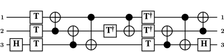
Figure 5.1. Toffoli circuit with 7 $T$ gates [3]. Our computer search shows that this circuit is $T$-optimal: Toffoli cannot be implemented using 3 qubits with less than $7$ T gates.

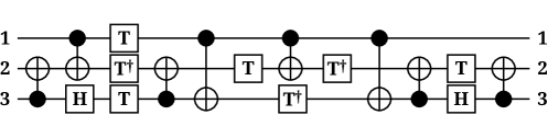
Figure 5.2. Fredkin circuit with $7$ $T$ gates [3]. Our computer search shows that this circuit is $T$-optimal.

6. Conclusions and open problems

Our algorithm for COUNT-T can be viewed as a method of performing exhaustive search. In contrast, in the single-qubit case we can characterize the $T$-count as a simple property of the given unitary: the $\mathrm{sde}$ of its channel representation. This characterization does not appear to generalize to $n>1$ qubits; for example, the $\mathrm{sde}$ of the channel representation of the Toffoli gate is $2$ but its $T$-count is 7.

We conclude by stating the most obvious question, which remains open: does there exist a polynomial time (as a function of $N$ and $m$) algorithm for COUNT-T? Alternatively, is this problem computationally difficult? We do not know the answer to this question even for the special case of two-qubit unitaries.

7. Acknowledgments

We thank Matthew Amy for helpful discussions. David Gosset is supported by NSERC. Michele Mosca is supported by Canada’s NSERC, MITACS, CIFAR, and CFI. IQC and Perimeter Institute are supported in part by the Government of Canada and the Province of Ontario.

Appendix A Proof of Fact 1

Proof.

We first show that it is sufficient to prove the result with $P=Z_{(1)}$. To see this, consider $P_{A},P_{B}\in\mathcal{P}_{n}\setminus\{\mathbb{I}\}$ and suppose we can efficiently compute circuits for Cliffords $C_{A},C_{B}\in\mathcal{C}_{n}$ which satisfy $C_{A}Z_{(1)}C_{A}^{\dagger}=P_{A}$ and $C_{B}Z_{(1)}C_{B}^{\dagger}=P_{B}$. Then $C_{B}C_{A}^{\dagger}P_{A}C_{A}C_{B}^{\dagger}=P_{B}$, and we can efficiently compute the circuit for $C_{B}C_{A}^{\dagger}$.

By conjugating with $\mathcal{O}(n)$ SWAP gates and CNOT gates (both are Clifford) we can map $P=Z_{(1)}$ into any operator of the form

(A.1) $$\bigotimes_{i=1}^{n}Z_{(i)}^{y_{i}}$$

with $\vec{y}\neq\vec{0}$ an $n$-bit string. This can be seen using the fact that

$$\text{CNOT}\left(\mathbb{I}\otimes Z\right)\text{CNOT}=Z\otimes Z$$

and

$$\text{SWAP}\left(\mathbb{I}\otimes Z\right)\text{SWAP}=Z\otimes\mathbb{I}.$$

Finally, note that the single-qubit Pauli $Z$ matrix can be mapped to either $X$ or $Y$ by single-qubit Cliffords $H\in\mathcal{C}_{1}$ and $T^{2}H\in\mathcal{C}_{1}$

$$HZH=X\qquad\left(T^{2}H\right)Z\left(T^{2}H\right)^{\dagger}=Y.$$

Using these facts it is not hard to see that $P=Z_{(1)}$ can be transformed into $P^{\prime}\in\mathcal{P}_{n}\setminus\{\mathbb{I}\}$ by first mapping to an operator of the form A.1 by conjugating with $\mathcal{O}(n)$ CNOTs and SWAPs, and then conjugating by a tensor product of (at most $n$) single-qubit Cliffords. ∎

References

• [1] Scott Aaronson and Daniel Gottesman. Improved simulation of stabilizer circuits. Physical Review A, 70(5):052328, 2004.
• [2] M. Amy, D. Maslov, and M. Mosca. Polynomial-time T-depth Optimization of Clifford+T circuits via Matroid Partitioning. e-print arXiv: 1303.2042, March 2013.
• [3] Matthew Amy, Dmitri Maslov, Michele Mosca, and Martin Roetteler. A meet-in-the-middle algorithm for fast synthesis of depth-optimal quantum circuits. Computer-Aided Design of Integrated Circuits and Systems, IEEE Transactions on, 32:818–830, 2013.
• [4] A. R. Calderbank, E. M Rains, P. W. Shor, and N. J. A. Sloane. Quantum Error Correction via Codes over GF(4). eprint arXiv:quant-ph/9608006, August 1996.
• [5] Brett Giles and Peter Selinger. Exact synthesis of multiqubit clifford+ T circuits. Physical Review A, 87(3):032332, 2013.
• [6] D. Gottesman. The Heisenberg Representation of Quantum Computers. eprint arXiv:quant-ph/9807006, July 1998.
• [7] C. Jones. Low-overhead constructions for the fault-tolerant Toffoli gate. Physical Review A, 87(2):022328, February 2013.
• [8] Vadym Kliuchnikov. Synthesis of unitaries with clifford+T circuits. eprint arXiv: 1306.3200, 2013.
• [9] Vadym Kliuchnikov, Dmitri Maslov, and Michele Mosca. Fast and efficient exact synthesis of single qubit unitaries generated by clifford and T gates. eprint arXiv: 1206.5236, 2013.
• [10] V. Veitch, S. A. Hamed Mousavian, D. Gottesman, and J. Emerson. The Resource Theory of Stabilizer Computation. e-print arXiv: 1307.7171, July 2013.