Evidence of a Binary-Induced Spiral from an Incomplete Ring Pattern of CIT 6

Abstract

With the advent of high-resolution high-sensitivity observations, spiral patterns have been revealed around several asymptotic giant branch (AGB) stars. Such patterns can provide possible evidence for the existence of central binary stars embedded in outflowing circumstellar envelopes. Here, we suggest the viability of explaining the previously observed incomplete ring-like patterns with the spiral-shell structure due to the motion of (unknown) binary components viewed at an inclination with respect to the orbital plane. We describe a method of extracting such spiral-shells from an incomplete ring-like pattern to place constraints on the characteristics of the central binary stars. The use of gas kinematics is essential in facilitating a detailed modeling for the three-dimensional structure of the circumstellar pattern. We show that a hydrodynamic radiative transfer model can reproduce the structure of the HC₃N molecular line emission of the extreme carbon star, CIT 6. This method can be applied to other sources in the AGB phase and to the outer ring-like patterns of pre-planetary nebulae for probing the existence of embedded binary stars, which are highly anticipated with future observations using the Atacama Large Millimeter/submillimeter Array.

1 INTRODUCTION

Binary motion is now well known to generate a spiral pattern in the circumstellar envelope of a mass losing star (Soker, 1994; Mastrodemos & Morris, 1999; He, 2007; Edgar et al., 2008; Kim, 2011; Kim & Taam, 2012a, b, c). However, it is not generally recognized that the binary-induced pattern, vertically extended from the orbital plane, exhibits a ring-like pattern with an inclined viewing angle. At an inclination close to edge-on, in particular, the binary-induced spiral-shell appears as eccentric arcs in the plane of the sky (see e.g., Mastrodemos & Morris, 1999; He, 2007; Kim & Taam, 2012b). Even at a low inclination (close to face-on), the pitch angle of the spiral pattern decreases with radius from the center of binary orbital motion (Kim & Taam, 2012b), such that the outer part of the spiral approximates a concentric ring structure. This misidentification may occur, especially, for the outer ring-like patterns of (pre-)planetary nebulae (PPN/PN) whose inner parts are contaminated by the bright, fast-moving lobes (e.g., NGC 7027 (Bond, 1996), Egg Nebula (Sahai et al., 1998)). Because of the incompleteness of the observed ring-like patterns, whether they arise from spherical shells due to the pulsation of single stars or spiral-shell patterns due to binary orbital motion is inconclusive. In this paper, we focus on the interpretation that the incomplete ring-like patterns observed in the past may be caused by the motion of (unknown) binary stars.

Linking a binary scenario with the ring-like patterns observed on the circumstellar envelopes of asymptotic giant branch (AGB) stars and their remnant material in the outer parts of PPN/PN has an interesting implication for the late phases of stellar evolution. Since the bipolar (often multi-polar) structures, including jets and tori, observed in the PPN/PN (e.g., Balick & Frank, 2002; Sahai et al., 2011) likely originate from the central binary systems (Morris, 1987; Huggins, 2007; De Marco, 2009), a fundamental issue remains concerning the origin of the ring-like patterns in the outer parts of the PPN/PN. Such a ring-like pattern is commonly assumed as the consequence of the periodic mass loss of a single star in the previous AGB phase, due to stellar pulsation (e.g., Willson & Hill, 1979; Wood, 1979) or thermal pulsation (e.g., Mattsson et al., 2007) on the spherically symmetric wind. For example, the archetypal AGB star, IRC+10216, reveals the circumstellar pattern in the optical and infrared images (Leão et al., 2006; Decin et al., 2011), which is characterized by an interval corresponding to $\sim$ 250–1700 years. Interestingly, Decin et al. (2011) noted that this pattern interval of IRC+10216 does not agree with either the stellar pulsation (649 days, Le Bertre, 1992) or the thermal pulsation (6000–33000 years, Ladjal et al., 2010). Similar discrepancy has also been found in several PPN/PN (Su, 2004). A binary-induced spiral-shell model, in which the pattern interval time is defined by the binary orbital period without a strong limitation on the scale, may possibly serve as an alternative explanation for the ring-like (but not perfectly symmetric) patterns formed in the AGB phase.

In the binary model, the observed spiral-shell pattern of a circumstellar envelope can constrain the binary mass and orbital properties. For the carbon-rich AGB star, AFGL 3068, displaying a well-defined spiral circumstellar pattern in dust scattered light, Mauron & Huggins (2006) estimated the orbital period simply from the arm interval and wind expansion speed, ignoring the inclination. For another carbon star, R Sculptoris, exhibiting a spiral pattern in addition to a thin thermal pulse shell, Maercker et al. (2012) characterized the thermal pulsation with the help of their modeled binary properties for the spiral pattern features. Similarly, the circumstellar patterns in close binary systems may be used in determining the relative importance and observational consequence of the accretion disks surrounding the companion star, as theoretically investigated (e.g., Theuns & Jorissen, 1993; Nordhaus & Blackman, 2006). Furthermore, Huarte-Espinosa et al. (2013) found that the bow shock around a disk can lead to complicated time-dependent post-shock structures for orbital separations less than about 20 AU. As such, the features of a spiral-shell pattern provide indirect evidence for the presence of a binary companion to the AGB star. In cases where the companion is obscured by the circumstellar envelope, the detection of spiral features may be the only diagnostic probe for, otherwise hidden binary systems.

In a previous paper (Kim & Taam, 2012c), we took account of the effect of inclination angle, for the first time, in modeling an observed circumstellar pattern within the binary framework. It was shown that the elongated spiral shape in the plane of the sky, seen in dust scattered light, can be used to constrain key binary quantities (i.e., inclination of the orbital plane, orbital period, companion mass, and mass ratio). However, this analysis left a degeneracy in such model parameters since the apparent shape in the plane of the sky reflects both the binary motion and projection effect due to the inclination of the orbital plane. In this paper, we show that the degeneracy can be lifted by using gas kinematics from high resolution observations, which provide three-dimensional information. To illustrate the modeling method, we apply the model to the object, CIT 6, by revisiting its incomplete ring-like pattern observed in molecular line emission with the spiral-shell due to the motion of (hypothesized) central binary stars.

In Section 2, we introduce the known properties of CIT 6 and the existing molecular line observation with the Very Large Array (VLA), which are used to constrain the model parameters. In Section 3, we formulate a simple analytic model based on the oblate spheroid geometry of an Archimedes spiral-shell with a binary orbital inclination $i$. This simple analytic model can be easily applied to other sources in order to ascertain whether a spiral-shell pattern exists. In Section 4, a parameter space analysis is carried out following the method of Kim & Taam (2012c) based on the elongated shape of the pattern in the plane of the sky. In Section 5, the results of hydrodynamic radiative transfer simulations are presented, from which we use molecular line kinematics to resolve the degeneracy in the parameter space analysis. We find that the simulated spiral-shell model can reproduce the observational data in the channel maps and position-velocity (P-V) diagrams, providing a better fit than obtained by using a spherically symmetric shell model. In Section 6, we discuss the advantage and limitation of the current model. Finally in Section 7, we summarize our findings and suggest future applications.

2 KNOWN FACTS OF CIT 6 AS MODEL CONSTRAINTS

CIT 6 (also known as RW LMi, IRC+30219, IRAS 10131+3049, AFGL 1403) is an extreme carbon star and believed to be in the transition from the AGB to the post-AGB phase. Schmidt et al. (2002) found the presence of a nascent bipolar nebula, providing evidence that the evolutionary phase of CIT 6 lies just pass the tip of AGB. Its effective temperature of 2800 K (Cohen, 1979) and the bolometric luminosity of $\sim 10^{4}\,L_{\sun}$ (Loup et al., 1993) also correspond to the values at the tip of AGB phase of the evolutionary track for a star with the initial mass of 2–3 $M_{\sun}$, according to the Single Stellar Evolution package of Hurley et al. (2000) assuming a solar metallicity. The distance to CIT 6 is estimated to be $400\pm 50$ pc based on the pulsation period ($1.65\pm 0.02$ yr) using a period-luminosity relation (Cohen & Hitchon, 1996, and references therein).

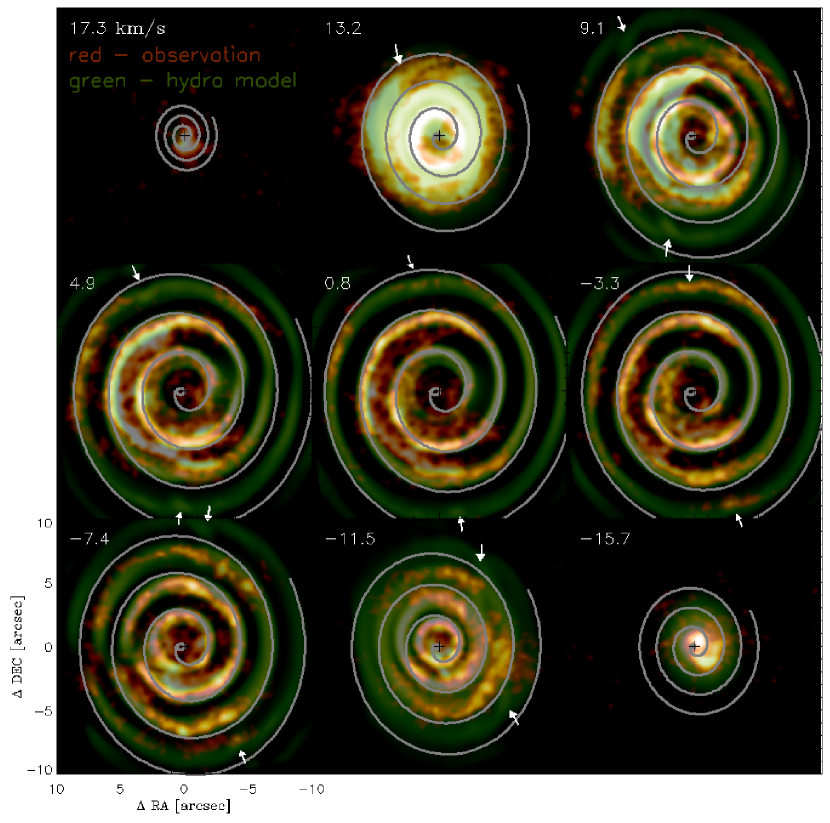
Figure 1: Velocity channel images of the HC₃N(4–3) line emission of CIT 6 observed with the VLA (red, Figure 1 of Claussen et al., 2011), and modeled by an hydrodynamic radiative transfer simulation using the FLASH and SPARX codes (green). The red color ranges from 1 to 5 mJy/beam logarithmically. In order to show the pattern shape in the model beyond the detection limit of this particular observation, the scale of the green color is displayed from 0.1 to 2 mJy/beam logarithmically with a synthetic beam size of $\sim 0.\!\!\arcsec 7$ and velocity resolution of $\sim 1\,\mbox{$\rm km\,s^{-1}$}$. North is up, and east is left. The position angles of the knots found in the hydrodynamic model are indicated by arrows. A simple geometric model with an inclined Archimedes spiral-shell is drawn by a gray solid line in each channel. The model parameters are summarized in Table 1.

The importance of CIT 6 stems from the existence of partial rings of molecular line emission based on VLA interferometric observational data obtained by Claussen et al. (2011, see also the red-scaled image in Figure 1) at high angular resolution ($\sim 0.\!\!\arcsec 7$) and high spectral resolution ($\sim 1\,\mbox{$\rm km\,s^{-1}$}$). Claussen et al. (2011) modeled this line emission pattern with four spherical shells, using the shell radii, expansion velocities, and central velocities as free parameters for the individual shells. Their model fitting results in different central velocities between the modeled shells, which may imply the departure from spherical symmetry of the circumstellar pattern about the central AGB star. Claussen et al. (2011) remarked on the existence of the asymmetric features such as the spiral shape (relatively well traced in the velocity channel of $-7.4\,\mbox{$\rm km\,s^{-1}$}$), stronger emission observed in the redshifted side, and lack of emission in the west and northwest near the central channels. Chau et al. (2012) showed that the optical depth effect cannot reproduce the asymmetric line profile of CIT 6 for a physical structure assumed to be spherically symmetric. Their three-dimensional morphokinematic model instead suggested several incomplete shells for the structure of CIT 6.

Here we suggest an alternative interpretation for the asymmetric shape of the circumstellar pattern as an indication for a central binary star system. Some evidence for binarity is indeed found in the Hubble Space Telescope (HST) images with two compact cores separated by $0.\!\!\arcsec 17$ at the position angle (PA, measured from north to east) of 10° (Monnier et al., 2000). The northern lobe varies in its flux and polarization with the known pulsation period of the carbon star ($1.65\pm 0.02$ yr; Cohen & Hitchon, 1996), while the bluer southern lobe is stable and has a polarization direction $\sim 90\arcdeg$ different from the northern red component (Trammell & Goodrich, 1997). These characteristics of the southern lobe, differing from those of the carbon star and the northern lobe, suggest that the blue southern lobe is illuminated by a companion star in the vicinity (Monnier et al., 2000). The existence of a companion star is supported by the consistence of the polarization direction of H_α emission (Trammell et al., 1994) to the blue component. From the observed flux at 4500Å, Schmidt et al. (2002) inferred that the companion is likely later than spectral type G0 ($\gtrsim 1$ $M_{\sun}$) if it is a main-sequence star.

3 ANALYTIC MODEL USING GEOMETRY OF INCLINED ARCHIMEDES SPIRAL-SHELL

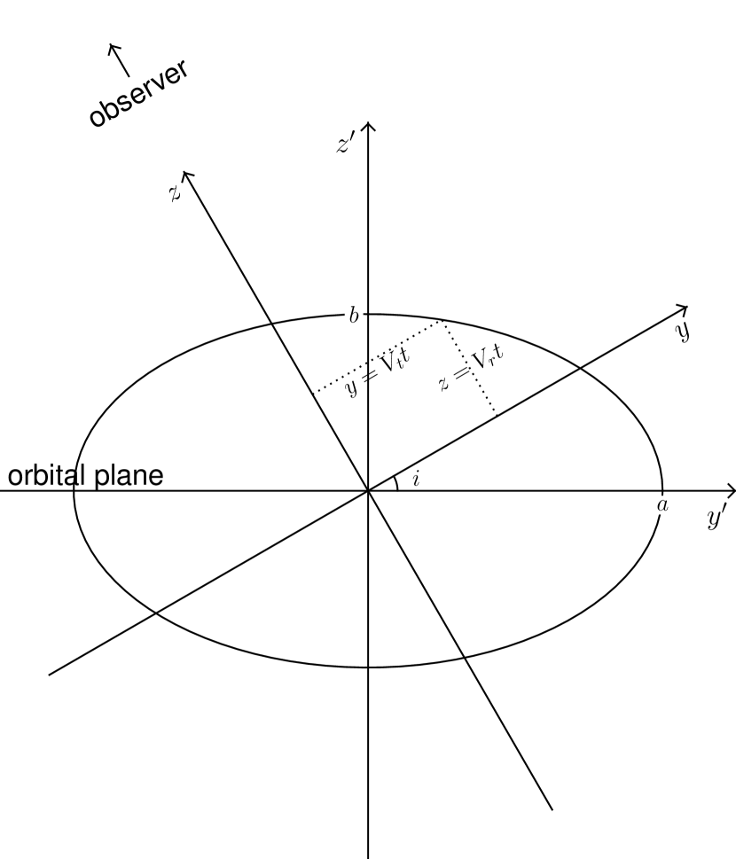
Figure 2: A schematic diagram of an oblate spheroid viewed by an observer with an inclination angle $i$, depicting the geometry in the prime (intrinsic) and unprime (observational) coordinate frames.

The orbital motion of a mass losing star in a binary system creates a spiral-shell pattern in its circumstellar envelope (e.g., Soker, 1994). We consider the overall morphology of the spiral-shell pattern as an oblate spheroid, following Kim & Taam (2012c). In the coordinates having the vertical axis $z^{\prime}$ aligned with the orbital axis, the oblate spheroid can be described by (see Figure 2)

$$(x^{\prime}/a)^{2}+(y^{\prime}/a)^{2}+(z^{\prime}/b)^{2}=1{,}$$ (1)

where the axial ratio $a/b$ is defined by the ratio of pattern propagation speeds $\mbox{$V_{\rm arm}$}/\mbox{$\langle V_{w}\rangle$}$ in the orbital plane and along the polar axis. Here, the radial propagation speed of the spiral pattern in the orbital plane is affected by the orbital motion of the mass losing star with the orbital speed of $V_{1}$ to be $\mbox{$V_{\rm arm}$}=\mbox{$\langle V_{w}\rangle$}+2V_{1}/3$ (Kim & Taam, 2012b), while the pattern propagation speed along the orbital axis is the average wind speed $\langle V_{w}\rangle$ corresponding to the intrinsic wind speed.

We define new coordinates $(x,\,y,\,z)$ rotated by an inclination $i$, in which the observer is at infinity in the direction of the $z$-axis. A rotational transformation about the $x$-axis by the angle $i$ is defined by $x^{\prime}=x$, $y^{\prime}=y\cos i+z\sin i$, and $z^{\prime}=-y\sin i+z\cos i$. Substitution of these into Equation (1) yields

$$R^{2}(1+f\sin^{2}i\,\sin^{2}\phi)+z^{2}(1+f\cos^{2}i)=a^{2},$$ (2)

where $R$ and $\phi$ refer to the tangential coordinate $R=(x^{2}+y^{2})^{1/2}$ and the azimuthal angle in the $x$–$y$ plane, respectively, defining $x=R\cos\phi$ and $y=R\sin\phi$. A factor $f$ is defined as $f=(a/b)^{2}-1$, thus

$$f=(\mbox{$V_{\rm arm}$}/\mbox{$\langle V_{w}\rangle$})^{2}-1.$$ (3)

Alternative forms of Equation (2) are

$$R=a(1+f\sin^{2}i\,\sin^{2}\phi)^{-1/2}\left(1-(z/a)^{2}(1+f\cos^{2}i)\right)^{1/2},$$ (4)

or

$$z=a(1+f\cos^{2}i)^{-1/2}\left(1-(R/a)^{2}(1+f\sin^{2}i\,\sin^{2}\phi)\right)^{1/2}.$$ (5)

Because the oblate spheroid geometry originates from the latitudinal variation of the wind velocity, these coordinates $R$ and $z$ can be linearly transformed to the tangential and line-of-sight velocities of the wind. Thus, the tangential component is

$$V_{t}= \mbox{$V_{\rm arm}$}\times(1+f\sin^{2}i\,\sin^{2}\phi)^{-1/2}$$ (6)

$$\times(1-(V_{r}/\mbox{$V_{\rm arm}$})^{2}(1+f\cos^{2}i))^{1/2},$$

representing the pattern propagation speed in the inclined plane within the $V_{r}$-channel. The second term in the right-hand-side of Equation (6) shows the inclination effect, and the last term is related to the channel velocity representing the height of the relevant material from the midplane. From Equation (6), the line-of-sight velocity can be written as

$$V_{r}= \mbox{$V_{\rm arm}$}\times(1+f\cos^{2}i)^{-1/2}$$ (7)

$$\times(1-(V_{t}/\mbox{$V_{\rm arm}$})^{2}(1+f\sin^{2}i\,\sin^{2}\phi))^{1/2},$$

at a given $V_{t}$. The maximum line-of-sight velocity is

$$(V_{r})_{\rm max}=\mbox{$V_{\rm arm}$}\times(1+f\cos^{2}i)^{-1/2},$$ (8)

at the orbital center (i.e., at the center of mass in the circular orbit case).

A circumstellar spiral pattern due to the orbital motion of the AGB star (orbital radius $r_{1}$; orbital velocity $V_{1}$) for a given $z$ is defined by a differential equation in the polar coordinates $(R,\,\phi)$ as,

$$\frac{1}{r_{1}}\frac{{\it d}R}{{\it d}\phi}=\frac{V_{t}}{V_{1}},$$ (9)

where the tangential velocity $V_{t}$ represents the pattern propagation velocity in the layer within the $V_{r}$-channel. The velocity $V_{t}$ is given by Equation (6) as a function of $\phi$ with given wind velocity, orbital velocity, and inclination angle. As the velocity of an AGB wind is nearly constant beyond the wind acceleration region (typically less than several times the stellar radius; Höfner, 2007), the integrated form of Equation (9) well approximates to

$$\left(\frac{R}{1\arcsec}\right)=\left(\frac{V_{t}}{V_{1}}\right)\left(\frac{r_{1}}{1\rm AU}\right)\left(\frac{d}{1\rm pc}\right)^{-1}\left(\frac{\phi}{1\rm rad}\right){,}$$ (10)

for the pattern located at a large radius $R$. Here, $d$ is the distance to the source.

4 PARAMETER SPACE ANALYSIS

In order to obtain approximate constraints on the binary properties, we explore the possible parameter space for the system of interest, following the method described in Kim & Taam (2012c) using an overall oblate spheroidal morphology of the pattern. Four observed quantities are required, corresponding to the projected axial ratio $(a/b)_{\rm proj}$, the arm pattern spacing $\Delta r_{\rm arm}$ along the major axis, the projected binary separation $(r_{1}+r_{2})_{\rm proj}$, and the angular position of the stars relative to the major axis of the elliptical pattern shape $\phi_{\rm binary,proj}=\rm PA_{binary,proj}-PA_{node}$. Here, $\rm PA$ refers to a position angle measured from the north to the east direction and hereafter $\phi$ is defined as the angle relative to the line of nodes of the binary orbit ($\rm PA_{node}$; the intersection of the orbital plane with the plane of the sky) measured in the counterclockwise direction. Refer to Kim & Taam (2012c) for the details of this method using an overall oblate spheroid shape.

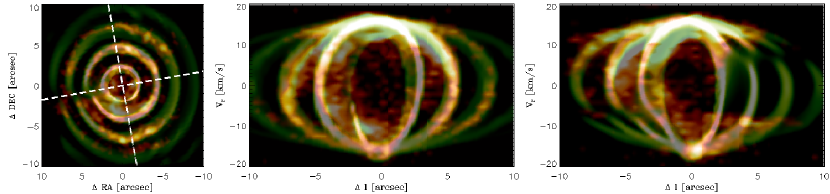
Figure 3: The HC₃N(4–3) line emission of CIT 6 taken with VLA (red, Claussen et al., 2011) compared with a spiral-shell model (green). A channel map at $-7.4\,\mbox{$\rm km\,s^{-1}$}$ includes white dashed lines for the major and minor axes at $\rm PA=10\arcdeg$ and 100° (left), along which the P-V diagrams present a relatively symmetric pattern (middle, $\rm PA=10\arcdeg$) and the most asymmetric pattern (right, $\rm PA=100\arcdeg$), respectively. The radius along the major and minor axes, $\Delta l$, is measured from bottom to top and left to right, respectively. The model parameters are tabulated in Table 1. The modeled orbit inclination is 60°. The red and green colors ranges from 1 to 5 mJy/beam and 0.1 to 2 mJy/beam, respectively, in a logarithmic scale.

We first identify the line of nodes of the binary orbit as the major axis of the elongated spiral pattern of the HC₃N(4–3) line emission in Figure 1. Because of the insufficient sensitivity of observation, it is challenging to precisely determine the angular direction of the major axis only by ellipse fitting. Thus, we also use the fact that the P-V diagram is most symmetric along the line of nodes and most asymmetric in the perpendicular direction (middle and right panels of Figure 3, respectively; see also Section 5.2). From the resulting ellipse fit with the major axis at $\rm PA_{node}=10\arcdeg$, we measure the axis ratio $(a/b)_{\rm proj}$ of 1.15 and the pattern spacing $\Delta r_{\rm arm}$ of $3.\!\!\arcsec 2$ along the major axis. We assume the two compact components from the optical images are members of a binary (or their surrounding gaseous envelopes) following Monnier et al. (2000), which provides a projected separation of $(r_{1}+r_{2})_{\rm proj}=0.\!\!\arcsec 17$ and a position angle of the binary at $\rm PA_{binary,proj}=10\arcdeg$. The line of nodes nearly coincides with the alignment of the two stars, implying that $(r_{1}+r_{2})_{\rm proj}$ is approximately equivalent to the actual binary separation. In addition to these four observed quantities, the distance of 400 pc is adopted (see Section 2), thus constraining the binary properties in a parameter space spanning the average wind velocity $\langle V_{w}\rangle$ versus the orbital velocity $V_{1}$ of the mass losing star (Figure 4).

The gray-colored area in Figure 4 shows the possible sets of binary parameters. The first constraint for the gray area is the mass of the evolved carbon star ($M_{1}$, black solid line) greater than the mean mass of white dwarfs (Madej et al., 2004). In particular, the stellar luminosity of $\sim 10^{4}\,L_{\sun}$ for CIT 6 suggests the core mass of $\sim 0.69\mbox{$M_{\sun}$}$ with 2% accuracy based on Paczyński (1971), providing the lower limit on the current mass, $M_{1}$, of the AGB star. The other constraint stems from the maximum line-of-sight velocity of the pattern $(V_{r})_{\rm max}$ corresponding to the half width of the HC₃N(4–3) line, measured as 18 $\rm km\,s^{-1}$ with an uncertainty of $\pm 0.5\,\mbox{$\rm km\,s^{-1}$}$ considering the spectral resolution. In previous papers (Kim & Taam, 2012b, c), the lower limit of the maximum line-of-sight velocity was loosely constrained by the condition $(V_{r})_{\rm max}\lesssim\mbox{$\langle V_{w}\rangle$}+V_{1}$, which is satisfied at any inclination. We further calculate the maximum line-of-sight velocity taking account of the inclination effect. From equation (8), the measured line-of-sight velocity range $(V_{r})_{\rm max}=18\pm 0.5\,\mbox{$\rm km\,s^{-1}$}$ is marked in Figure 4 as a set of yellow dotted lines.

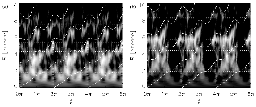
Figure 5: The HC₃N(4–3) line emission in the channel velocity of (a) $-7.4\,\mbox{$\rm km\,s^{-1}$}$ (left bottom in Figure 1) and (b) $0.8\,\mbox{$\rm km\,s^{-1}$}$ (middle in Figure 1) plotted in the polar coordinates. An elongated spiral model is drawn by dashed lines, tracing the wiggle feature. For comparison, an Archimedes spiral without the inclination effect (i.e., face-on) appears to have a constant slope in the polar coordinates, connecting the local peaks of the dashed lines. Dotted lines refer to the four spherical shell model in Claussen et al. (2011). The gray color ranges from 1 to 5 mJy/beam in a logarithmic scale.

The plausibility of a particular model parameter set can be easily checked by the simple analytic model in Section 3. Among the possible models in Figure 4, the parameter set marked by a plus symbol is applied to the analytic model. The model consists of an estimate of the AGB star mass of $M_{1}=0.8\,\mbox{$M_{\sun}$}$, companion mass $M_{2}=2.2\,\mbox{$M_{\sun}$}$, binary separation $r_{1}+r_{2}=68$ AU, inclination $i=60\arcdeg$, and average wind velocity $\mbox{$\langle V_{w}\rangle$}=15.7\,\mbox{$\rm km\,s^{-1}$}$ with the distance $d=400$ pc. The result is overlaid in each velocity channel map of Figure 1 by a gray-colored solid line, showing a reasonable match with the outer edge of the observed pattern (red-scaled), particularly for the middle-row panels displaying the near-central velocity channels. Furthermore, this inclined spiral can explain the wiggle feature of the observed pattern in the polar coordinates, clearly seen in Figure 5. Without considering the inclination effect (i.e., assuming face-on; $i=0$), the pattern propagation speed $V_{t}$ in each $V_{r}$-velocity channel is constant in Equation (6), indicating that the pattern should appear as a straight line in the polar coordinates with the slope determined by Equation (10). For comparison, a concentric spherical shell pattern forms horizontal lines in the $\phi$-$R$ coordinates in Figure 5. Therefore, the wiggle feature, which is also found in other sources (e.g., R Sculptoris, see Figure 2a in Maercker et al., 2012), is a natural outcome of the inclined spiral model, and is distinguishable from the face-on view of the spiral model for a binary system and the spherical shell model for a single star.

5 HYDRODYNAMIC RADIATIVE TRANSFER MODEL

The region delineated by the gray-colored area in the parameter space (Figure 4), based on the elongated spiral shape projected on the plane of the sky, can be sharpened by taking advantage of three-dimensional information provided by the molecular line kinematics. We explore the parameter space in the vicinity of the $(V_{r})_{\rm max}=18$ $\rm km\,s^{-1}$ line with hydrodynamic simulations followed by radiative transfer calculations for the HC₃N molecular line. The parameters for the model which best matches the aspects of the VLA observation (Claussen et al., 2011), described in Sections 5.2 and 5.3, are summarized in Table 1 (and by a plus sign in Figure 4). We note that these parameters are not independent of each other due to their constraints imposed by the parameter space analysis.

5.1 Numerical method

The basic equations of hydrodynamics are integrated using the FLASH3 code (Fryxell et al., 2000) based on a piecewise parabolic method (Colella & Woodward, 1984). We construct a centrally concentrated, static grid utilizing the block-structured adaptive mesh refinement PARAMESH package and adjusting the refinement level based on the distance from the stars. The maximum refinement level of eight with the grids of $64\times 64\times 32$ per block is used for the simulation domain of 8400 AU$\times$8400 AU$\times$4200 AU ($21\arcsec\times 21\arcsec\times 10.\!\!\arcsec 5$ at 400 pc, corresponding to the image size of the VLA observation in consideration) in three-dimensional Cartesian coordinates, assuming the mirror symmetry about the orbital $x$–$y$ plane. The spatial gridding corresponds to a resolution of 1 AU ($0.\!\!\arcsec 0025$) in the central region, assigning a sufficient number of grid cells at the wind generating radius $r_{\rm in}$ within which physical conditions are reset every simulational timestep, in order to assure the ejection of gas from the mass losing star in a spherical shape. The gas temperature over the simulation domain is scaled by the temperature $T_{\rm in}$ at the wind generating radius $r_{\rm in}$ from the mass losing star. We set $r_{\rm in}=\rm 10\,AU$, and $T_{\rm in}$ is calculated by the temperature distribution $T(r)=T_{\rm eff}(r/r_{\rm eff})^{-2(\gamma-1)}$ of an adiabatic gaseous medium with a $r^{-2}$ density distribution. The observed effective temperature $T_{\rm eff}=\rm 2800\,K$ is set at the assumed stellar photospheric radius $r_{\rm eff}=556\,R_{\sun}$ or 2.59 AU. An adiabatic equation of state with the adiabatic index $\gamma$ of 1.4 is used.

The gravitational potentials of the stars are treated as Plummer potentials (see, e.g., Binney & Tremaine, 2008) using the POINTMASS implementation of the FLASH3 code with modifications to include the gravitational softening radii and the motion of the two stars. The gravitational softening radius of the mass losing star does not change the result as it is smaller than the wind generating radius. The gravitational softening radius of the companion is set to be comparable to the Hoyle-Lyttleton accretion radius. An additional simulation with the companion’s softening radius reduced by a factor of 2 is compared with the model presented in this paper, in order to verify its insignificant contribution to the overall shape of the arm pattern. The accretion disk of the companion is expected to have a negligible size if it is gauged by the impact parameter (0.004 AU with the large separation of our binary system) in Huarte-Espinosa et al. (2013). Resolving the accretion disk for a wide binary system is computationally very expensive and beyond the scope of this paper.

The FLASH3 results are used as inputs to the radiative transfer calculation for HC₃N lines with the SPARX code. SPARX, standing for Simulation Package for Astrophysical Radiative Transfer, is a software package for calculating molecular excitation and radiative transfer of (dust) continuum and molecular lines at millimeter/submillimeter wavelengths. It adopts the accelerated Monte Carlo (AMC) algorithm developed by Hogerheijde & van der Tak (2000), and finds full non-local thermodynamical equilibrium (non-LTE) solutions of molecular level population and radiation fields iteratively and consistently. Instead of assuming that the molecular excitation is simply in equilibrium corresponding to the local temperature, non-LTE demands only statistical equilibrium of the level population through collisional and radiative excitation and de-excitation processes, which can be solved with the detailed balance equation. Additional (de-)excitation mechanisms, such as infrared radiative pumping, have not been incorporated in the package.

As a post-processing tool, the SPARX requires inputs of molecular gas density, temperature, velocity as well as the linewidth distribution, which can be provided by the results of a hydrodynamic simulation. Knowledge of the molecular abundance distribution and parameters such as dipole moments, line frequencies, and collisional rates are also required by the SPARX. The final SPARX output includes synthetic images which can be used for generating spectra and P-V diagrams, as input for a telescope filter for simulated observations, or for other scientific analysis. Details of the package such as the code implementation and its verification with benchmark cases will be presented in Liu et al. (2013, in preparation).

For the SPARX calculation, the HC₃N molecular parameters are obtained from the Leiden Atomic and Molecular Database (LAMDA) (Schöier et al., 2005). The HC₃N abundance of $1.5\times 10^{-6}$ is adopted throughout the envelope (Zhang et al., 2009), while a spherical central region of 2″ was carved out with HC₃N abundance set to zero in order to mimic the central hole seen in the observed emission of HC₃N (also found in its parent molecule CN; Lindqvist et al., 2000). For computational efficiency, we use the spatial and spectral resolutions of $0.\!\!\arcsec 13$ and 0.4 $\rm km\,s^{-1}$ in the SPARX calculation, which are sufficient to simulate the VLA observation of Claussen et al. (2011) summarized in Section 2. To further compare the SPARX output with the VLA observation, we perform a convolution with a Gaussian beam of $0.\!\!\arcsec 7$ and the rebinning to 1 $\rm km\,s^{-1}$ over the synthetic images.

5.2 Inclination effects on line kinematics

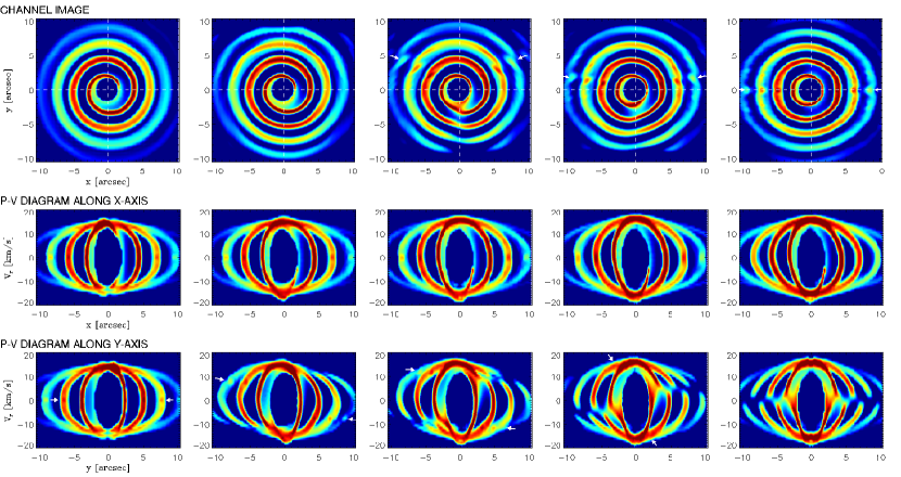
Figure 6: The HC₃N(4–3) line emission distribution for the binary system in Table 1 with the inclination of 0° (face-on), 30°, 50°, 70°, and 90° (edge-on) from left to right. The top panels display the images for the $-7.4\,\mbox{$\rm km\,s^{-1}$}$ channel, while the middle and bottom panels show the P-V diagram along $x$- and $y$-axis, respectively. The line of nodes of the binary orbits ($x$-axis; major axis) corresponds to $\rm PA=10\arcdeg$ in Figure 1. Attention is in the changes of position angle of knotty structure in both channel image and P-V diagram (marked by arrows), the tilt of pattern in the P-V diagram along $y$-axis at mid-range inclinations, and the increase of maximum velocity with inclination. The color ranges from 0.1 to 2 mJy/beam in a logarithmic scale from blue to red, for the synthetic beam size of $\sim 0.\!\!\arcsec 7$ and velocity resolution of $\sim 1\,\mbox{$\rm km\,s^{-1}$}$.

The inferred binary parameters are sensitive to the orbital inclination as illustrated in Figure 4. Hence, determination of the inclination can lift the degeneracy that remain in the parameter space analysis based only on the pattern shape in the plane of the sky. With the binary parameters in Table 1, Figure 6 compares the images for the non-zero velocity channels and the P-V diagrams along the major (i.e., $x$-axis; line of nodes) and minor (i.e., $y$-axis; perpendicular to the line of nodes) axes for five different inclinations of 0° (face-on), 30°, 50°, 70°, and 90° (edge-on). The channel images (top row) illustrate the change of pattern shape from a spiral in the face-on view to ellipses in the edge-on view. In particular, the spiral pattern is split along $-y$-axis in the image for $i=50\arcdeg$ and attached to the adjacent component in the image for $i=70\arcdeg$, making a new ring.

The P-V diagrams of Figure 6 (middle and bottom rows) reveal notable features. The middle row show that, regardless of inclination, the P-V diagram along the line of nodes (i.e., $x$-axis) appears relatively symmetric about the central velocity because of the mirror symmetry of the overall oblate spheroid geometry about the orbital plane. In contrast, the P-V diagram along the minor axis highly depends on the inclination angle (bottom row). One important implication is that the PA dependence of the P-V diagram can be used to determine the line of nodes of the binary orbit (as in Section 4). Moreover, the comparison between the P-V diagrams along major and minor axes helps to infer the inclination angle of the system from the observed data cube. For example, the PA dependence of the P-V diagram is minimized in the face-on case.

The P-V diagram along the minor axis (bottom row) provides further information on the orbital inclination. At a mid-range inclination (see e.g. $i=30\arcdeg$), it reveals an asymmetry in intensity between the redshifted and blueshifted components, the degree of asymmetry of which differs with position, and thus the overall shape of P-V diagram is tilted. Hence, the degree of tilt and spectral asymmetry is dependent on the inclination. On the other hand, the maximum line-of-sight velocity (i.e., $V_{r}$ at $x=y=0$) increases with inclination as predicted in Equation (8). This increase of maximum velocity makes the outline of P-V diagram at the high end velocity at each $y$ position ($|V_{r}|\gtrsim 10\,\mbox{$\rm km\,s^{-1}$}$) shallower in the face-on case ($i=0\arcdeg$) and becoming steeper as the inclination increases. All these features of the P-V diagrams can be used to constrain the inclination angle of the binary system.

In the framework of the binary model, the companion creates a gravitationally-induced density wake in a flatter spiral shape, overlapped with the spiral-shell pattern due to the orbital motion of the AGB star (Kim & Taam, 2012b). The overlapped region appears as knots in the plane of the sky at the PA depending on the inclination (See Figure 10 of Kim & Taam, 2012b) because the knots represent the companion’s wake relatively thin in the vertical direction from the orbital plane (Kim & Taam, 2012a). In Figure 6, the top panels for a non-zero velocity channel show such knots at high inclinations ($i\gtrsim 50\arcdeg$ in this model) at the PA varying with the inclination (marked by arrows). In the P-V diagram along the minor axis (bottom row), knots appearing with low inclinations ($i\lesssim 50\arcdeg$) also shift the positions depending on the inclination. On the other hand, in the P-V diagram along the line of nodes of orbits (middle row) all knotty structures are present at the zero velocity, confirming the existence of the companion’s wake on the orbital plane.

In short, the shape of P-V diagram, the degree of spectral asymmetry, the position of knots both in individual channels and in individual P-V diagrams provide important clues in identifying the best model. It is also worth noting that the velocity dispersion of individual arm component is dominated by the velocity variation due to the binary orbital motion ($\sim 4.6\,\mbox{$\rm km\,s^{-1}$}$). For the binary system in Table 1 with an inclination angle of 60°, the above features reasonably match the VLA observation.

5.3 Fiducial model

Figure 1 shows the modeled HC₃N(4–3) line emission with the parameters in Table 1 in green color, overlaid with the observational data displayed in red color. A good correlation exhibits between the observed and modeled data in the individual velocity channels, albeit the outermost arm in the observation is barely detected at the $3\sigma$ level, where the noise level $\sigma=0.5$ mJy/beam refers the root-mean-square of the line-free channels in the VLA observation. The observed channel images (red) range between 1 and 5 mJy/beam. To present the pattern shape beyond the sensitivity limit of the observation, the modeled channel images (green) are displayed from 0.1 to 2 mJy/beam.

All arc patches in the observed line emission are well located on the modeled spiral pattern. At the central channels (middle panels of Figure 1) the model reveals elongated spiral patterns, while at higher velocity channels (top and bottom panels) ring-like patterns are reproduced. Here, we emphasize that the ring-like features appear in the spiral-shell models with considerably large inclination angles (see Kim & Taam, 2012b). It suggests that ring-like patterns observed in the AGB circumstellar envelopes and in the outer parts of PPN/PN do not necessarily imply an underlying spherically symmetric nature. The inclination angle of the presented model is 60°.

The binary model in Figure 1 shows the breakup of rings and their unequal spacing between adjacent arms. This appears in the intermediate range of inclination angles, reflecting the transition from a spiral shape to a ring shape, as explained in Section 5.2. In the $-7.4\,\mbox{$\rm km\,s^{-1}$}$ channel, for example, the ring-like pattern is incomplete revealed by the gap in the east at $\rm PA=100\arcdeg$ (along the east side of minor axis; see also the first panel of Figure 3). The ring radius of the northern part of the gap is larger than the radius of the southern part, in which the model and observation match sensibly.

The companion’s gravitational wake appears as knots in the modeled channel images located in specific PAs (marked by arrows in Figure 1) as determined by the inclination. In the zero-velocity channel (middle panel of Figure 1) representing the midplane, the knots are arranged along the line of nodes of the orbits (i.e., $\rm PA=10\arcdeg$ and 190°). The knots shift to the east in the redshifted velocity channels and to the west in the blueshifted channels. The direction of shift of the knots with the channel velocity is determined by the orientation of the companion’s orbit. The model knots eventually converge on the east and west ends of the ring pattern at the maximum velocity channels, which results in the thickening and brightening of the pattern at such locations.

The PAs of knots in the modeled channel images are consistent with bright emission spots in the corresponding VLA images. For example, the observed image (in Figure 1) exhibits thickening and brightening features in the ring pattern on the east and west ends at the $13.2\,\mbox{$\rm km\,s^{-1}$}$ and $-11.5\,\mbox{$\rm km\,s^{-1}$}$ channels, respectively. Another example is found at the southwest in the $-3.3\,\mbox{$\rm km\,s^{-1}$}$ and $-7.4\,\mbox{$\rm km\,s^{-1}$}$ channels, where the detected emission in the outermost ring (red) corresponds to the position of bright knotty structure in the model (green). At the locations of these knots, the arm (in red and green images) is found considerably inside the analytic Archimedes spiral model without considering the companion’s gravitational wake (gray solid line). This decrease of arm radii is explained by Kim & Taam (2012b, Figure 9 and text), which showed that a shock front (appearing as knots in the channel images) at the location of the companion’s wake reduces the speed of the downstream flow and, therefore, the pattern propagation speed.

6 DISCUSSION

We have shown that a numerical hydrodynamic radiative transfer model for CIT 6 demonstrates that the observed incomplete ring patches can be naturally understood within the framework of a single spiral-shell pattern induced by a binary motion. In contrast, the previous spherical shell model (Claussen et al., 2011) and incomplete shell model (Chau et al., 2012) required the use of individual shell parameters without providing physical understanding for their variations. Moreover, the binary model reveals that the knotty structures result from the overlapping between a spiral-shell shaped pattern due to the orbital motion of the mass losing star and a more flattened spiral pattern onto the orbital plane due to the companion’s motion. In this picture, the knots are aligned in a specific PA, which systematically changes with the velocity channel. This implies that such regularly-aligned knots are a natural consequence of the model.

The total flux integrated over the full simulation domain is related to the mass loss rate and the HC₃N abundance for a given temperature distribution. We have adopted the mass loss rate of $3.2\times 10^{-6}\,\mbox{$\mbox{$M_{\sun}$}\rm\,yr^{-1}$}$ and relative molecular abundance of $1.5\times 10^{-6}$  from Zhang et al. (2009). Unlike Zhang et al. (2009), who assumed the local thermal equilibrium with a single temperature, the temperature distribution in our model is determined by an adiabatic gas equation of state. The resulting total flux is smaller than the VLA observation by a factor of 2. This implies that a complete modeling of these parameters requires studies involving a further fine-tuning of the input parameters as well as the introduction of molecular chemistry. Such studies will also necessitate incorporating observations of various molecular species, transitions, and angular resolutions. However, these parameters merely scale the flux level, but do not change the shape of the spiral pattern which is the focus of this paper.

The fact that the observed redshifted emission component is stronger than the blueshifted component is, however, not reproduced in our spiral model, albeit a small magnitude of spectral asymmetry is found depending on the inclination. This implies that our model is incomplete and that the asymmetry along the line-of-sight does not originate solely from the binary motion. The observed spectral asymmetry may agree with a presence of a bow shock due to the interaction between the circumstellar and interstellar media if the space motion away from us is significant (e.g., Wilkin, 1996; Wareing et al., 2006; Mayer et al., 2011). However, the VLA data does not show a shift of the Local Standard of Rest (LSR) velocity from the central velocity of the spiral-shell pattern. Other possible effects which may enhance the asymmetry include physical and chemical inhomogenities in the surrounding matter or in the dust formation phase at the onset of the stellar wind (e.g., Soker, 2000; Woitke & Niccolini, 2005) if propagated to large scales.

The missing emission in the west side of the central channels is also beyond the scope of this paper. This observed feature cannot be explained simply by a spiral-shell model nor by a spherical shell model. This spatial asymmetry is also found in a different transition of HC₃N and in its parent molecule CN (Lindqvist et al., 2000; Dinh-V.-Trung & Lim, 2009). We speculate that such lack of emission could possibly be caused by a chemical effect reducing the molecular abundance, rather than being affected by the gas density.

Compared to the other model sets in the parameter space determined by the projected pattern shape (Figure 4), for instance at $(V_{1},\,\mbox{$\langle V_{w}\rangle$})=(3.65,\,15.7)$, the presented model shows a better match with the observation for the pattern features explained in Section 5.2–5.3 in both channel maps and P-V diagrams. However, the difference of our fiducial model from the other comparison model sets are not decisive for the given uncertainties in the model parameters. In particular, observational uncertainties due to the limited sensitivity in determining the elongated shape and the arm spacing, as well as the determination of the source distance, stellar luminosity, photospheric temperature, and binary separation enter. Follow-up observations with a higher sensitivity for a chemically stable molecule such as CO would address some of these uncertainties.

7 SUMMARY

We have developed a method to investigate the incomplete ring-like feature of a spiral-shell pattern in an outflowing circumstellar envelope, due to the orbital motion of central binary stars with an inclination with respect to the orbital plane, providing an alternative explanation to models invoking periodic mass loss events of a single star. As a first step in this method, a parameter space study is performed as in Kim & Taam (2012c) and improved upon by taking account of the inclination angle for the constraint on the wind expansion velocity. The results of such an analysis significantly narrow down the parameter space that can provide a fit to the observed pattern shape in the plane of the sky. This reduction in the parameter space is important for the second step where a modest number of hydrodynamic and radiative transfer investigations can be carried out. The pattern shape, degree of asymmetry, position of knots in individual velocity channels and P-V diagrams are used via detailed modeling to constrain binary properties.

We have shown that gas kinematics is important in constraining the binary properties, which would otherwise remain degenerate under the constraints from the parameter space analysis based only on the shape of the circumstellar spiral-shell pattern in the plane of the sky. We have also demonstrated that a simple analytic analysis for the elongated spiral model based on an Archimedes spiral-shell pattern viewed as a function of inclination angle for comparison to individual velocity channels is useful for determining the applicability of the model to observational data. Finally, observed circumstellar patterns often reveal wiggles with varying slope in the polar coordinates that can be adequately described by the elongated spiral model, not by a face-on Archimedes spiral nor by spherical shells.

We have used the AGB star, CIT 6, as the first example to illustrate a method which can be used to help to constrain the binary properties given the existence of high resolution and sensitivity VLA data for the HC₃N(4–3) molecular line. This first success of applying the binary-induced spiral-shell model to an observed incomplete ring-like pattern opens the possibility of connecting the ring-like patterns commonly found in the AGB circumstellar envelopes and in the outer parts of PPN/PN and pointing to the conceivable presence of central binary systems.

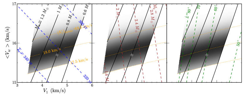
Figure 4: Model parameter space of the undisturbed wind velocity $\langle V_{w}\rangle$ versus the orbital velocity $V_{1}$ of the mass losing star in a binary system, based on the shape of an elongated spiral pattern with the projected axial ratio of 1.15, the arm spacing of 1280 AU ($3.\!\!\arcsec 2$ at 400 pc), the binary stars aligned with the line of nodes of orbits with the separation of 68 AU ($0.\!\!\arcsec 17$). Black solid lines represent the current mass $M_{1}$ of the mass losing star. Yellow dotted lines show the half of linewidth of $18\pm 0.5\mbox{$\rm km\,s^{-1}$}$, constraining the model binary system within the gray-colored region favoring the darker area. The binary orbital period, the companion mass $M_{2}$, the orbit inclination $i$ are displayed by blue, red, and green dashed lines in left, middle, and right panels, respectively. Plus sign corresponds to a binary model for $M_{1}=0.8\,\mbox{$M_{\sun}$}$, $M_{2}=2.2\mbox{$M_{\sun}$}$, and $i=60\arcdeg$ with the separation of 68 AU, and the line-of-sight expansion velocity of 17.8 $\rm km\,s^{-1}$.

Table 1: Model parameters

$M_{1}$	$M_{2}$	$r_{1}+r_{2}$	$i$	$\langle V_{w}\rangle$		$T_{\rm in}$	$r_{\rm in}$	$\gamma$		$\dot{M}_{1}$	HC3N abundance
[$M_{\sun}$]	[$M_{\sun}$]	[AU]	[deg]	[$\rm km\,s^{-1}$]		[$K$]	[AU]			[$\mbox{$M_{\sun}$}\rm\,yr^{-1}$]	[of H2]
0.8	2.2	68	60	15.7		950	10	1.4		$3.2\!\times\!10^{-6}$	$1.5\!\times\!10^{-6}$

Note. — Current mass of mass losing star $M_{1}$, mass of its companion $M_{2}$, their separation $r_{1}+r_{2}$, orbit inclination $i$, and intrinsic wind velocity from the mass losing star $\langle V_{w}\rangle$ are chosen based on the parameter space analysis as indicated with the plus sign in Figure 4. The modeled binary stars are currently located at the line of node ($\phi_{\rm binary}=0\arcdeg$). $T_{\rm in}$ refers the temperature at reference position, $r_{\rm in}$, representing the wind formation radius. $\gamma$ is the adiabatic index of gas. The mass loss rate $\dot{M}_{1}$ and HC₃N abundance are taken from Zhang et al. (2009).

References

- Balick & Frank (2002) Balick, B., & Frank, A. 2002, ARA&A, 40, 439
- Binney & Tremaine (2008) Binney, J., & Tremaine, S. 2008, Galactic Dynamics (Princeton, NJ: Princeton Univ. Press)
- Bond (1996) Bond, H. 1996, HST press release STScI-PR96-05
- Colella & Woodward (1984) Colella, P., & Woodward, P. R. 1984, Journal of Computational Physics, 54, 174
- Chau et al. (2012) Chau, W., Zhang, Y., Nakashima, J.-i., Deguchi, S., & Kwok, S. 2012, ApJ, 760, 66
- Claussen et al. (2011) Claussen, M. J., Sjouwerman, L. O., Rupen, M. P., et al. 2011, ApJ, 739, L5
- Cohen (1979) Cohen, M. 1979, MNRAS, 186, 837
- Cohen & Hitchon (1996) Cohen, M., & Hitchon, K. 1996, AJ, 111, 962
- Decin et al. (2011) Decin, L., Royer, P., Cox, N. L. J., et al. 2011, A&A, 534, A1
- De Marco (2009) De Marco, O. 2009, PASP, 121, 316
- Dinh-V.-Trung & Lim (2009) Dinh-V.-Trung, & Lim, J. 2009, ApJ, 701, 292
- Edgar et al. (2008) Edgar, R. G., Nordhaus, J., Blackman, E. G., & Frank, A. 2008, ApJ, 675, L101
- Fryxell et al. (2000) Fryxell, B,. Olson, K., Ricker, P., et al. 2000, ApJS, 131, 273
- He (2007) He, J. H. 2007, A&A, 467, 1081
- Höfner (2007) Höfner, S. 2007, Why Galaxies Care About AGB Stars: Their Importance as Actors and Probes, 378, 145
- Hogerheijde & van der Tak (2000) Hogerheijde, M. R., & van der Tak, F. F. S. 2000, A&A, 362, 697
- Huggins (2007) Huggins, P. J. 2007, ApJ, 663, 342
- Huarte-Espinosa et al. (2013) Huarte-Espinosa, M., Carroll-Nellenback, J., Nordhaus, J., Frank, A., & Blackman, E. G. 2013, MNRAS, 1448
- Hurley et al. (2000) Hurley, J. R., Pols, O. R., & Tout, C. A. 2000, MNRAS, 315, 543
- Kim (2011) Kim, H. 2011, ApJ, 739, 102
- Kim & Taam (2012a) Kim, H., & Taam, R. E. 2012a, ApJ, 744, 136
- Kim & Taam (2012b) Kim, H., & Taam, R. E. 2012b, ApJ, 759, 59
- Kim & Taam (2012c) Kim, H., & Taam, R. E. 2012c, ApJ, 759, L22
- Leão et al. (2006) Leão, I. C., de Laverny, P., Mékarnia, D., de Medeiros, J. R., & Vandame, B. 2006, A&A, 455, 187
- Ladjal et al. (2010) Ladjal, D., Barlow, M. J., Groenewegen, M. A. T., et al. 2010, A&A, 518, L141
- Le Bertre (1992) Le Bertre, T. 1992, A&AS, 94, 377
- Lindqvist et al. (2000) Lindqvist, M., Schöier, F. L., Lucas, R., & Olofsson, H. 2000, A&A, 361, 1036
- Loup et al. (1993) Loup, C., Forveille, T., Omont, A., & Paul, J. F. 1993, A&AS, 99, 291
- Madej et al. (2004) Madej, J., Należyty, M., & Althaus, L. G. 2004, A&A, 419, L5
- Maercker et al. (2012) Maercker, M., Mohamed, S., Vlemmings, W. H. T., et al. 2012, Nature, 490, 232
- Mastrodemos & Morris (1999) Mastrodemos, N., & Morris, M. 1999, ApJ, 523, 357
- Mattsson et al. (2007) Mattsson, L., Höfner, S., & Herwig, F. 2007, A&A, 470, 339
- Mauron & Huggins (2006) Mauron, N., & Huggins, P. J. 2006, A&A, 452, 257
- Mayer et al. (2011) Mayer, A., Jorissen, A., Kerschbaum, F., et al. 2011, A&A, 531, L4
- Monnier et al. (2000) Monnier, J. D., Tuthill, P. G., & Danchi, W. C. 2000, ApJ, 545, 957
- Morris (1987) Morris, M. 1987, PASP, 99, 1115
- Nordhaus & Blackman (2006) Nordhaus, J., & Blackman, E. G. 2006, MNRAS, 370, 2004
- Paczyński (1971) Paczyński, B. 1971, Acta Astron., 21, 271
- Sahai et al. (2011) Sahai, R., Morris, M. R., & Villar, G. G. 2011, AJ, 141, 134
- Sahai et al. (1998) Sahai, R., Trauger, J. T., Watson, A. M., et al. 1998, ApJ, 493, 301
- Schmidt et al. (2002) Schmidt, G. D., Hines, D. C., & Swift, S. 2002, ApJ, 576, 429
- Schöier et al. (2005) Schöier, F. L., van der Tak, F. F. S., van Dishoeck, E. F., & Black, J. H. 2005, A&A, 432, 369
- Soker (1994) Soker, N. 1994, MNRAS, 270, 774
- Soker (2000) Soker, N. 2000, MNRAS, 312, 217
- Su (2004) Su, K. Y. L. 2004, Asymmetrical Planetary Nebulae III: Winds, Structure and the Thunderbird, 313, 247
- Theuns & Jorissen (1993) Theuns, T., & Jorissen, A. 1993, MNRAS, 265, 946
- Trammell et al. (1994) Trammell, S. R., Dinerstein, H. L., & Goodrich, R. W. 1994, AJ, 108, 984
- Trammell & Goodrich (1997) Trammell, S. R., & Goodrich, R. W. 1997, AAS, 191, 47.15
- Wareing et al. (2006) Wareing, C. J., Zijlstra, A. A., Speck, A. K., et al. 2006, MNRAS, 372, L63
- Wilkin (1996) Wilkin, F. P. 1996, ApJ, 459, L31
- Willson & Hill (1979) Willson, L. A., & Hill, S. J. 1979, ApJ, 228, 854
- Woitke & Niccolini (2005) Woitke, P., & Niccolini, G. 2005, A&A, 433, 1101
- Wood (1979) Wood, P. R. 1979, ApJ, 227, 220
- Zhang et al. (2009) Zhang, Y., Kwok, S., & Dinh-V-Trung 2009, ApJ, 691, 1660