The Bolocam Galactic Plane Survey. X. A Complete Spectroscopic Catalog of Dense Molecular Gas Observed toward 1.1 mm Dust Continuum Sources with $7.5$^∘$\leq l\leq 194$^∘

Abstract

The Bolocam Galactic Plane Survey (BGPS) is a 1.1 mm continuum survey of dense clumps of dust throughout the Galaxy covering 170 square degrees. We present spectroscopic observations using the Heinrich Hertz Submillimeter Telescope of the dense gas tracers, HCO⁺ and N₂H⁺ $3-2$, for all 6194 sources in the Bolocam Galactic Plane Survey v1.0.1 catalog between $7.5$^∘$\leq l\leq 194$^∘. This is the largest targeted spectroscopic survey of dense molecular gas in the Milky Way to date. We find unique velocities for 3126 ($50.5$%) of the BGPS v1.0.1 sources observed. Strong N₂H⁺ $3-2$ emission ($T_{mb}>0.5$ K) without HCO⁺ $3-2$ emission does not occur in this catalog. We characterize the properties of the dense molecular gas emission toward the entire sample. HCO⁺ is very sub-thermally populated and the 3-2 transitions are optically thick toward most BGPS clumps. The median observed line width is $3.3$ km/s consistent with supersonic turbulence within BGPS clumps. We find strong correlations between dense molecular gas integrated intensities and $1.1$ mm peak flux and the gas kinetic temperature derived from previously published NH₃ observations. These intensity correlations are driven by the sensitivity of the $3-2$ transitions to excitation conditions rather than by variations in molecular column density or abundance. We identify a subset of 113 sources with stronger N₂H⁺ than HCO⁺ integrated intensity, but we find no correlations between the N₂H⁺/HCO⁺ ratio and 1.1 mm continuum flux density, gas kinetic temperature, or line width. Self-absorbed profiles are rare ($1.3$%).

1 Introduction

In the last few years, comprehensive surveys of the Milky Way galaxy have been performed at submillimeter and millimeter wavelengths that have imaged dust continuum emission and have provided the most complete census of embedded sites of star formation in our Galaxy. The Bolocam Galactic Plane Survey (BGPS) version 1.0 mapped over 170 square degrees of the Galactic plane at 1.1 mm (Aguirre et al. 2011) and has catalogued over 8400 continuum sources (Rosolowsky et al. 2010). The BGPS observed the entire first quadrant in a strip that is 1^∘ wide in galactic latitude with selected regions observed in the second ($l\approx$ 98^∘, 111^∘, 133^∘$-$ 136^∘), third (188^∘$\leq l\leq$ 192^∘) and fourth quadrants ($l>350$^∘). A complementary survey at 870 $\mu$m, ATLASGAL, has mapped sections of the southern Milky Way with a 2^∘ wide strip in galactic latitude between longitudes of $300$^∘$\leq l\leq 60$^∘ (Contreras et al. 2013). Also, the Herschel Space Observatory survey, Hi-Gal, has mapped the Galactic plane at 70, 160, 250, 350, and 500 $\mu$m (Molinari et al. 2012). When the complete ATLASGAL and Hi-Gal survey source catalogs are released and are combined with the BGPS catalogs, the final source catalog will contain tens of thousands of embedded sites of star formation in the Milky Way.

The population of objects discovered in the BGPS, ATLASGAL, and Hi-Gal surveys include dense starless and star-forming cores at the closest distances, clumps (unresolved collections of cores), and clouds at the farthest distances (Dunham et al. 2011a). In order to study the physical properties (e.g. size, mass, luminosity) of these embedded star-forming regions, their distances must first be determined. Distances in the Galactic plane may be derived using the Galactic rotation curve and a measurement of the source $v_{LSR}$. In the second and third quadrants, kinematic distances are uniquely determined; but, in the first and fourth quadrants, each measured $v_{LSR}$ corresponds to both a near and far kinematic distance resulting in a kinematic distance ambiguity that must be resolved using additional information.

Assignment of kinematic distances first and foremost requires a determination of the unique $v_{LSR}$ of the 1.1 mm clump. CO is too easily excited in low density molecular gas to be a unique kinematic probe ($n_{eff}<10^{2}$ cm^-3). Along lines-of-sight that cross multiple arms of the Galaxy, as often happens in the first quadrant of the Galaxy, CO $1-0$ emission displays complicated spectral shapes with multiple components spanning many tens of km/s. The gas directly associated with the clumps is best probed by a dense molecular gas tracer. Schlingman et al. (2011) performed a pilot survey of slightly less than 1/3 of the BGPS clumps (1882 sources) in the first and second quadrant of the Galactic plane in the dense gas tracers HCO⁺ and N₂H⁺ $3-2$ ($n_{eff}\sim 10^{4}$ cm^-3). They showed that HCO⁺ and N₂H⁺ $3-2$ are unique kinematic tracers of BGPS clumps with less than $2$% of sources observed displaying multiple velocity components. They also resolved the kinematic distance ambiguity of a small subset ($N=529$) of the BGPS clumps. Schlingman et al. (2011) found a median radius of 0.75 pc, a median mass of $320$ M_⊙, a median volume density of 2400 cm^-3, and a median gravitational free-fall time of 750,000 years for this subset of sources. The resulting clump mass distribution ($dN/d\log M$) had a slope of $-0.8$ that is intermediate between the CO cloud mass distribution ($-0.6$; Solomon et al. 1987) and the Salpeter IMF ($-1.35$; Salpeter 1955; Scalo 1986) and is consistent with simulations of the fragmentation of turbulent compressible gas with a Kolmogorov spectrum (i.e. Hennebelle & Falgarone 2012). Schlingman et al. also observed a breakdown in the size-linewidth in the dense molecular gas probed by HCO⁺, possibly due to turbulent feedback on small scales from embedded protostellar sources (see Murray et al. 2011). While the Schlingman survey provided an initial look the physical properties of BGPS clumps, the physical properties derived from the known distance sample in that paper represents less than $10$% of the full BGPS v1.0.1 catalog and is biased toward the brightest 1.1 mm sources.

In this paper, we complete the spectroscopic observations started by Schlingman et al. (2011) and provide a complete spectroscopic catalog of observations of dense molecular gas as traced by HCO⁺ and N₂H⁺ $3-2$ for all 6194 sources in the BGPS v1.0.1 catalog between $7.5$^∘$\leq l\leq 194$^∘. We characterize the properties of the molecular emission ($v_{LSR}$, I, $\Delta v$, etc.) for the spectroscopic catalog in this paper. A companion paper develops a Bayesian method for resolving the kinematic distance ambiguity for a subset of sources in the first quadrant by deriving Distance Probability Density Functions (DPDFs, Ellsworth-Bowers et al. 2013). The observing and calibration procedures are explained in §2, detection statistics are described in §3, and the source $v_{LSR}$ are extracted in §4.1. The properties of the molecular emission are analyzed in §4.2-§4.5.

2 Observations

2.1 HHT Setup and Calibration

4705 BGPS clumps in the range $7.5$^∘$\leq l\leq 194$^∘ were observed during $51$ observing shifts between February 28, 2011 and December 8, 2012 with the 10m Heinrich Hertz Telescope (HHT). The source catalog was determined by observing all Bolocat v1.0.1 sources that were not previously observed by Schlingman et al. (2011) plus re-observing sources where the pointing in Schlingman et al. exceeded half the HHT beamwidth ($15$″) from the v1.0.1 catalog peak 1.1 mm continuum position. Re-observation of a subset (393) of the Schlingman sources was necessary because the Schlingman et al. observations did not have access to the final v1.0.1 catalog positions, but were instead observed with an earlier (v0.7) version of the Bolocat (see §2.2). The observations in this paper are ultimately combined with the Schlingman et al. observations for sources with good correspondence to the v1.0.1 positions ($\Delta\theta<15$″). The resulting spectroscopic catalog is a complete set of observations of every source (6194) in the v1.0.1 Bolocat with $7.5$^∘$\leq l\leq 194$^∘.

The HHT observational procedure was similar to that used to observe the initial sample of 1882 BGPS clumps in Schlingman et al. (2011). Observations were performed with the 1mm prototype-ALMA dual polarization, sideband-separating receiver. The receiver was tuned to HCO⁺ $3-2$ (267.5576259 GHz) in the lower sideband (LSB) and to N₂H⁺ $3-2$ (279.5118379 GHz) in the upper sideband (USB). Rejection between the sidebands was measured by observing the bright Galactic source, W75(OH), for $10$ minutes each observing shift. The median rejections for the upper sideband were $-15.7$ dB and $-8.6$ dB for vertical and horizontal polarization respectively. The 4-IF output was connected to one set of filterbanks with 1 MHz spectral resolution and 512 MHz bandwidth. This spectral resolution corresponds to a velocity resolution of $1.12$ km/s in the LSB and $1.07$ km/s in the USB. Each source was observed in position-switching mode with 1 minute of ON-source integration time. Emission free OFF positions for every half-degree of the galactic plane were determined by Schlingman et al. (2011).

Observations at the HHT are placed on the $T_{A}^{*}$ scale using the standard Chopper-Wheel Calibration method (Penzias & Burrus 1973). Observations of planets are then used to determine the main beam efficiency and put the spectra on a final $T_{mb}^{pol}=T_{A}^{*}/\eta_{mb}\eta_{pol}$ scale, where $\eta_{mb}\eta_{pol}$ is the product of the telescope main beam efficiency and the coupling efficiency between the receiver optics for each polarization and the telescope. Unfortunately, during the bulk of the observing (47 out of 51 shifts), the only planet available for observation was Saturn. Saturn has two potential problems for calibration. First, the rings contribute to the 1.1 mm continuum and also block continuum from the planet. Fortunately though, the rings were oriented with inclinations between $7.3$^∘ and $9.8$^∘ which correspond to the shallow minimum in the millimeter brightness temperature (Weiland et al. 2011). Second, Saturn also has pressure broadened PH₃ $J_{K}=1_{0}-0_{0}$ emission at 267 GHz in the atmosphere (Encrenaz & Moreno 2002). The lower sideband (HCO⁺ $3-2$) calibration is strongly affected by this absorption and cannot be used to calibrate the main beam efficiency. The upper sideband (N₂H⁺ $3-2$) is much less affected by PH₃ absorption and was used to calibrate the upper sideband main beam efficiencies. Jupiter was available for observations only after June, 2011 and the ratio between lower sideband and upper sideband efficiencies was applied to the Saturn calibration to derive the lower sideband main beam efficiencies.

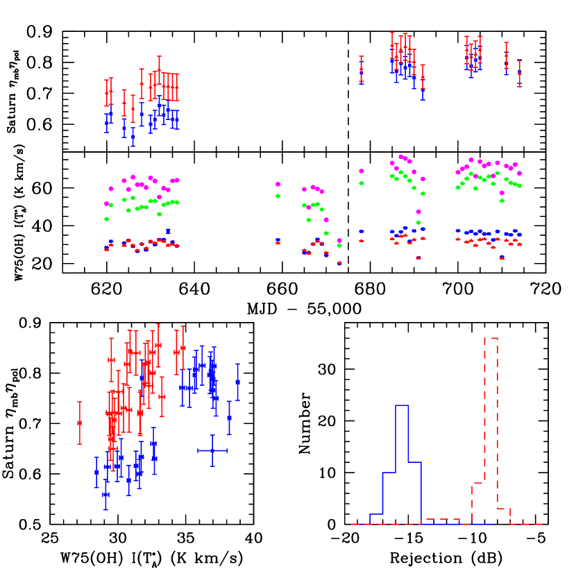
Figure 1: TOP: The main beam efficiency of the USB measured on Saturn and the integrated intensity of HCO⁺ $3-2$ (LSB) and N₂H⁺ $3-2$ (USB) emission observed toward W75(OH) for Hpol USB (blue squares), Vpol USB (red triangles), Hpol LSB (green pentagon), and Vpol LSB (magenta circle). Due to PH₃ absorption in Saturn’s atmosphere in the LSB, we only plot USB data for Saturn. The dashed line MJD-55,000 = 675 corresponds to a systematic change in the calibration associated with a warmup and adjustment of the receiver optics. BOTTOM LEFT: The USB main beam efficiency of Saturn is well correlated with integrated intensities measured for W75(OH). BOTTOM RIGHT: Histograms of the sideband rejection in the USB for Hpol (blue solid line) and Vpol (red dashed line).

As a consistency check, we also observed the source W75(OH) during every shift. The integrated intensity of W75(OH) correlates with the main beam efficiency measured using Saturn (Figure 1). A significant jump in the calibration is seen for both Saturn and W75(OH) at MJD = 55675 days. This discontinuity is due to a warmup of the receiver and subsequent adjustment of the feedhorn optics. The increase in efficiencies at this date occurs for all polarizations and sidebands simultaneously. The main beam efficiencies used in this paper are listed in Table 1. The final calibration numbers agree well with those used in Schlingman et al. The final spectrum is the baseline rms weighted-average of the calibrated vertical and horizontal polarizations $T_{mb}=(T_{mb}^{Vpol}/\sigma_{T^{Vpol}_{mb}}^{2}+T_{mb}^{Hpol}/\sigma_{T^{Hpol}_{mb}}^{2})/(1/\sigma_{T^{Vpol}_{mb}}^{2}+1/\sigma_{T^{Hpol}_{mb}}^{2}))$ .

2.2 A Note About BGPS Catalog Versions

A spectroscopic survey of a large number of sources, such as the one presented in this paper, requires using a fixed source catalog during the course of the survey. At the start of the Schlingman et al. (2011) observations in November 2008, the final BGPS v1.0 source catalog had not been completed, so Schlingman et al. utilized the preliminary Bolocat v0.7 catalog. The results from those early spectroscopic observations helped tune the inputs for the seeded-watershed algorithm ultimately used to generate the v1.0 catalog (Rosolowsky et al. 2010). At the beginning of this current survey in February 2011, the version 1.0.1 catalog was the latest version of the BGPS source catalog available and forms the basis for this paper. In February 2013, a re-reduction of the BGPS (version 2.0) became available (Ginsburg et al. 2013). Simulations and testing of the new pipeline reduction plus characterization of the BGPS v2.0 angular transfer function are reported in Ginsburg et al. (2013). The resulting v2.0 BGPS maps recover larger scale structure better than v1.0 maps. A new v2.0 source catalog using the same inputs for the seeded-watershed algorithm that was used to generate the v1.0.1 catalog is also now available; however, the source selection algorithm has not been optimized for the noise structure in the new v2.0 maps. The fluxes quoted throughout this paper are derived from the new v2.0 BGPS 1.1 mm images. Since these new data products only became available after spectroscopic observations were completed (December 2012), we shall reference all spectroscopic observations sequentially in this paper to the v1.0.1 source names and catalog numbers in the spectral properties table (Tables 2 and 3).

3 Detection Statistics

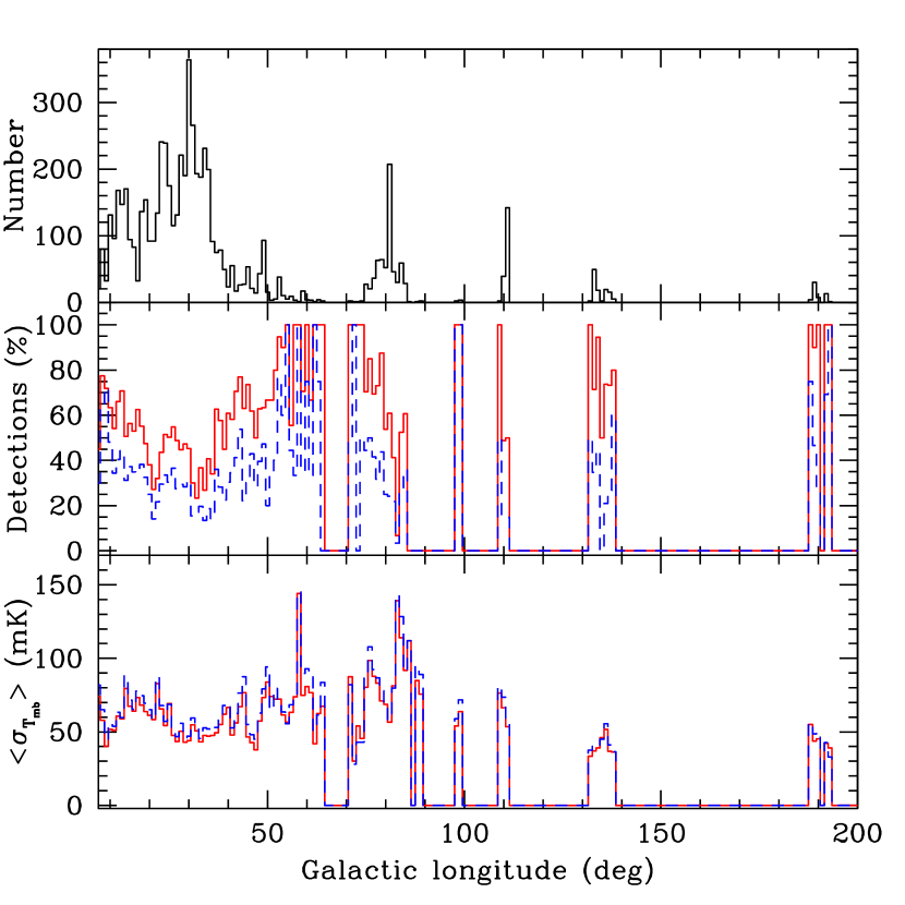
Figure 2: TOP: The distribution of BGPS v1.0.1 catalog sources with Galactic longitude. MIDDLE: Detection fraction for each Galactic longitude bin of HCO⁺ $3-2$ (solid red histogram) and N₂H⁺ $3-2$ detections (dashed blue histogram). BOTTOM: The distribution of the average baseline rms for HCO⁺ $3-2$ (red, solid line) and N₂H⁺ $3-2$ (blue, dashed line). Values of zero indicate l ranges with no sources. $\mbox{$\langle\sigma_{T_{mb}}\rangle$}=58$ mK for HCO⁺ $3-2$ and $\mbox{$\langle\sigma_{T_{mb}}\rangle$}=62$ mK for N₂H⁺ $3-2$ for the complete spectroscopic survey.

The complete spectroscopic survey reaches a mean baseline rms of $58$ mK for spectra in the LSB and $62$ mK for spectra in the USB. As a result, the mean $3\sigma_{T_{mb}}$ limits for HCO⁺ $3-2$ and N₂H⁺ $3-2$ in this survey are $0.174$ K and $0.186$ K respectively. During the best weather, baseline rms of $30$ mK were observed. The distribution of $\sigma_{T_{mb}}$ with Galactic longitude is shown in Figure 2.

Detections are confirmed visually, independently in each polarization, before the final spectrum is flagged. We adopt the flagging scheme in Schlingman et al. (2011) with two changes. We have eliminated the flag for large line wings (flag = $4$ in the Schlingman et al. scheme); sources in the Schlingman catalog with a flag of 4 have been re-classified with a flag of $1$ (single peak detection) or $3$ (self-absorbed profile) in the final catalog presented in this paper. Also, to eliminate numerical gaps in our flag scheme, we have re-classified all self-absorbed profiles in the Schlingman et al. catalog (originally a flag of $5$) as a flag of $3$. The flags in the merged catalog span from $0$ to $3$ and correspond to: a source with a flag = 1 indicates a single $v_{LSR}$ component detected at the $>3\sigma_{T_{mb}}$ level; a source with a flag = 2 indicates a multiple $v_{LSR}$ components detected; a source with a flag = 3 indicates a source with possible self-absorption; and a source with a flag = 0 indicates a non-detection.

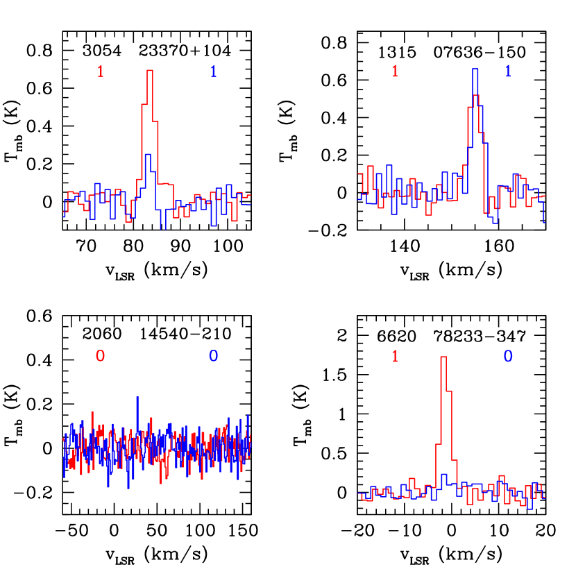
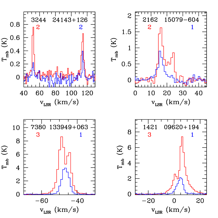
Figure 3: Example spectra showing different flag combinations. Red spectra are HCO⁺ $3-2$ and blue spectra are N₂H⁺ $3-2$. The Bolocat v1.0.1 source number is listed in the upper left of each panel while the truncated v1.0.1 catalog source name is listed in the top right of each panel. The HCO⁺ $3-2$ flag is shown in red below the source number on the left while the N₂H⁺ $3-2$ flag is shown in blue below the source name on the right. The majority of detections are similar to source 3054 (G23.370+0.104). Source 1315 (G07.636-0.150) is an example of a N₂H⁺ brighter source. Source 6620 (G78.233-0.347) is an example of a HCO⁺ detection and a N₂H⁺ non detection. Source 2060 (G14.540-0.210) is a non detection in both lines. Note that the velocity scale for the non-detections source 2060 spans the full range of plausible $v_{LSR}$ for a source at $l=14.5$^∘. The spike near 30 km/s in the G14.540-0.210 N₂H⁺ spectrum is not a detection as it is only one channel wide and does not appear independently in both polarizations. Sources 3244 (G24.143+0.126) and 2162 (G15.079-0.604) show examples of multiple $v_{LSR}$ components where N₂H⁺ peaks in one or both velocity components. The two self-absorbed profiles (sources 7380 and 1421) show examples of blue and red asymmetries in the HCO⁺ $3-2$ profiles respectively with the N₂H⁺ $3-2$ spectra peaking near the self-absorption minima.

Examples of spectra with different flag combinations are shown in Figure 3. The vast majority of detections are similar to source 3054 (G23.370+0.140) with a single Gaussian peak in both HCO⁺ and N₂H⁺ $3-2$ (HCO⁺ flag = $1$ and N₂H⁺ flag = $1$). Source 1315 (G07.636-0.150) is an example of a N₂H⁺ detection that is stronger than a HCO⁺ detection while source 6620 (G78.233-0.347) is an example of a HCO⁺ detection and a N₂H⁺ non-detection. Source 2060 (G14.540-0.210) is an example of a non-detection in both lines over the full velocity range permissible for objects at $l=14$^∘ ($-60$ to $+160$ km/s). The four panels on the right of Figure 3 display examples of detections with multiple velocity peaks. Source 3244 (G24.143+0.128) shows two clearly separated velocity peaks ($\Delta v_{LSR}=60$ km/s) indicative of two physically separate dense clumps along the same line-of-sight. Occasionally, the two peaks are blended. In the case of source 2162 (G15.079-0.604), the N₂H⁺ $3-2$ spectrum peaks at the same velocity as one of the HCO⁺ $3-2$ peaks; therefore, we do not classify this source as a self-absorbed profile, but as multiple velocity components in HCO⁺ $3-2$ (HCO⁺ flag = $2$). The two panels on the bottom right of Figure 3 show examples of blue-skewed and red-skewed self-absorbed HCO⁺ $3-2$ profiles where the N₂H⁺ $3-2$ emission does peak near the self-absorption minima (HCO⁺ flag = $3$).

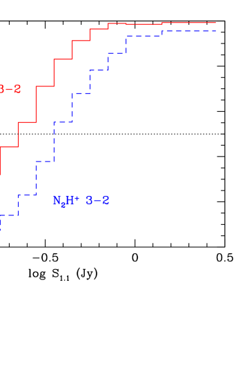
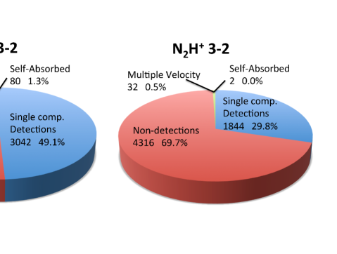
Figure 4: TOP: The detection fraction for HCO⁺ $3-2$ (red solid line) and N₂H⁺ $3-2$ (blue dashed line) versus 1.1 mm flux densities derived from the v2.0 BGPS maps at the location of the HHT pointing position. The HCO⁺ $3-2$ detection fraction is above 50% for 1.1 mm flux densities $>200$ mJy. BOTTOM: Detection flag statistics for HCO⁺ and N₂H⁺ $3-2$ for 6194 sources in the complete spectroscopic catalog.

The detection fractions for each spectroscopic flag are summarized in pie charts in Figure 4. HCO⁺ $3-2$ emission was detected toward a total of $3206$ ($51.8$%) sources. N₂H⁺ $3-2$ emission was detected toward a smaller fraction, $1878$ ($30.3$%) sources. Multiple velocity components are rare in these dense gas tracers with $84$ HCO⁺ $3-2$ multiple velocity detections ($1.3$%) and $32$ N₂H⁺ $3-2$ multiple velocity detections ($0.5$%). There are only $4$ N₂H⁺ $3-2$ detections ($0.06$%) that lack a corresponding HCO⁺ $3-2$ detection. None of these four unique N₂H⁺ $3-2$ detections are very significant, only ranging from $T_{mb}^{pk}=(3-5)\sigma_{T_{mb}}$. As an example, source 1705 (G012.387+00.230) has a $3.7\sigma$ detection in $T_{mb}$ for N₂H⁺ $3-2$ but there is a potential HCO⁺ 3-2 detection at only $2.9\sigma$ which falls just short of the criteria set in this paper for a HCO⁺ detection flag = 1. Strong N₂H⁺ $3-2$ emission without an HCO⁺ $3-2$ detection does not occur for the BGPS sources observed in this spectroscopic catalog. Therefore, we have observed a unique velocity component for $3126$ sources ($50.5$%) in the Bolocat v1.0.1 within the range $7.5$^∘$\leq l\leq 194$^∘.

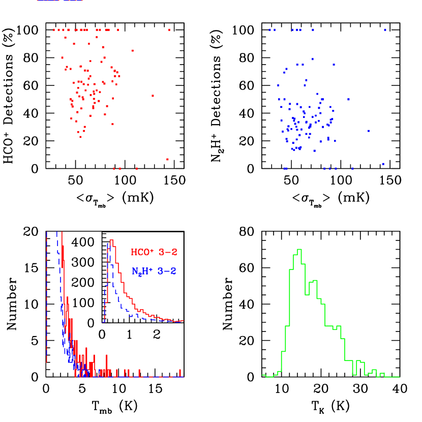
Figure 5: TOP PANELS: The HCO⁺ $3-2$ (LEFT) and N₂H⁺ $3-2$ (RIGHT) detection fraction plotted versus average baseline rms per $1$^∘ bin in Galactic longitude. BOTTOM LEFT: The main beam brightness temperature for HCO⁺ $3-2$ (red solid line) and N₂H⁺ $3-2$ (blue dashed line). We have truncated the histograms at 3K to better display the peak of each distribution. BOTTOM RIGHT: The histogram of gas kinetic temperature from the overlap NH₃ sample.

The distributions of $T_{mb}$ for both tracers are shown in Figure 5. Both histograms peak just above the $3\sigma_{T_{mb}}$ limit indicating that deeper integration is likely to detect more sources in the lines of HCO⁺ and N₂H⁺ $3-2$. The total observing time for the complete spectroscopic survey is $>600$ hours; a modest decrease of a factor of two in the rms noise level would require four times longer than the current survey. The detection statistics are a function of Galactic longitude in this survey (see Figure 2). The detection fraction does not strongly correlate with the baseline rms in the survey (Figure 5). For instance, the region near $l=30$^∘ which has the largest number of 1.1 mm sources within a $1$^∘ bin has a detection fraction of only $30$% despite having small baseline rms compared to the entire survey ($\sigma_{T_{mb}}=40$ mK). An opposite example can be found at $l=83$^∘ where a higher baseline rms results in a lower detection fraction; however, these instances are rare in this survey.

In order to understand this result, we must first compare the detection statistics to the flux density of BGPS sources. The detection fraction is a strong function of the $1.1$mm flux density of BGPS sources (Figure 4). v1.0.1 sources with $1.1$mm flux densities below 200 mJy have a less than $50$% detection percentage with the detection fraction decreasing rapidly below this flux density. This flux density corresponds to a column density limit of $N_{H_{2}}=4\times 10^{21}$ cm^-2 assuming a dust temperature of 20 K, gas mass to dust mass ratio of 100:1, and Ossenkopf & Henning opacities ($\kappa_{1.1}^{\rm{OH5}}=1.14$ cm² g^-1; Ossenkopf & Henning 1994). In contrast, sources with flux densities above 500 mJy have a detection fraction approaching $90$% (N${}_{H_{2}}\geq 1\times 10^{22}$ cm^-2). These variations in detection fraction with Galactic longitude primarily represent variations in the number of low flux density sources selected by the Bolocat seeded-watershed algorithms in different, sometimes crowded, regions of the Galactic plane (see Figure 17 of Rosolowsky et al. 2010). The region toward $l=30$^∘ contains a larger fraction of low flux density ($S_{1.1}<200$ mJy) sources than other regions in the Galactic plane resulting in the lower overall detection fraction. This $l=30$^∘ region of the Galactic plane is crowded and confused as the observed line-of-sight crosses the Sagittarius arm, the tangent of the end of the molecular bar, Perseus arm, and an outer Galactic arm.

We can test the fidelity of low flux density sources in the v1.0.1 catalog by directly comparing to the detection statistics with the new v2.0 catalog. For sources with no v2.0 catalog counterpart within $60$″ of the v1.0.1 source position (1813 sources), the HCO⁺ $3-2$ non-detection fraction (HCO⁺ flag = 0) increases from $48.0$% for the complete v1.0.1 catalog to $73.7$% for this subset. Nearly half of all v1.0.1 HCO⁺ $3-2$ non-detections are no longer directly associated with sources in the v2.0 catalog. Furthermore, those v1.0.1 sources that lack a v2.0 counterpart are predominantly low flux density v1.0.1 sources (Ginsburg et al., 2013) A significant fraction of low flux density v1.0.1 sources may not be real or are low volume density sources at the limit of statistical significance in the 1.1 mm map. Conversely, there are 476 v1.0.1 sources which have HCO⁺ $3-2$ detections (HCO⁺ flag = 1 or 3) but no nearby ($<60$″) counterpart in the v2.0 catalog. These results indicate that the v2.0 catalog has a better chance of selecting clumps with detectable dense molecular gas (at the limit of this spectroscopic survey) but that the v2.0 catalog is incomplete and misses a significant number of sources with dense molecular gas in the BGPS survey. This comparison only serves to highlight the difficulties inherent in source selection algorithms and also how surveys of dense molecular gas may be used to test the fidelity of those source catalogs.

4 Properties of Molecular Detections

In this section, we analyze the properties of the HCO⁺ and N₂H⁺ $3-2$ emission for the complete set of $3210$ spectroscopic detections. The spectra are analyzed using the same analysis techniques presented in Schlingman et al. (2011). Namely, a single component Gaussian is fit to HCO⁺ $3-2$ spectra while a multiple-component hyperfine fit is performed on N₂H⁺ $3-2$ spectra. In cases where a single component Gaussian fit fails or is not appropriate to described the observed line shape, the velocity of $T_{mb}^{pk}$ is reported. The integrated intensities ($I=\int T_{mb}dv$) are determined from direct integration of the spectra. Tables 2 and 3 list the derived spectroscopic properties ($\sigma_{T_{mb}}$, $v_{LSR}$, $T_{mb}^{pk}$, I, FWHM, and FWZI) for HCO⁺ and N₂H⁺ $3-2$ observations of all 6194 sources in the v1.0.1 catalog with $7.5$^∘$\leq l\leq 194$^∘.

In addition to the molecular lines observed in this survey, NH₃ is another popular dense gas tracer because it is easily excited in dense molecular gas and the ratio of the (1,1) and (2,2) inversion lines may be used to determine the gas kinetic temperature (Ho & Townes 1983). There have been two substantial Galactic NH₃ surveys published in the past two years. The Dunham et al. (2011) survey used the 100m Green Bank Telescope to follow-up a sample of 631 BGPS sources in the (1,1), (2,2), and (3,3) inversion lines. The Wienen et al. (2012) survey used the 100m Effelsberg Telescope (of which the inner 80m is practical for 1 cm NH₃ observations) to follow-up 862 ATLASGAL sources in the (1,1) and (2,2) inversion lines. We have directly compared the positions observed in the Dunham et al. and Wienen et al. NH₃ catalogs with the HHT pointing positions to find a subset of 546 sources with NH₃ pointings within $15$″ and having both published NH₃ detections and HCO⁺ $3-2$ detections. The distribution of gas kinetic temperatures for these 546 sources is shown in Figure 5. The median is $T_{k}=18.3$ K with a positively skewed tail of kinetic temperatures. We shall also use the gas kinetic temperature from this overlap subset of 546 sources in the subsequent analysis.

4.1 Kinematics of BGPS Sources

The primary purpose of this spectroscopic survey is to find a unique $v_{LSR}$ for each BGPS source. The $v_{LSR}$ for molecular detections is determined from a Gaussian fit to the HCO⁺ $3-2$ line for sources with a flag = $1$. Observations of N₂H⁺ $3-2$, when detected, provide an independent measurement of the velocity of dense molecular gas.

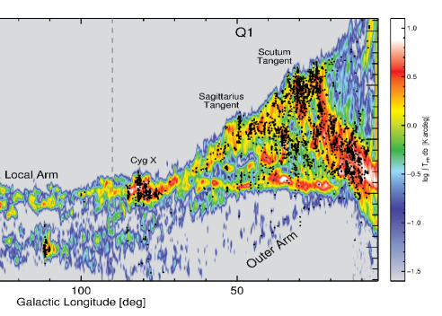
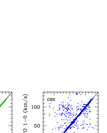
Figure 6: TOP: Velocities of BGPS clumps (black circles) overlaid on the CO $1-0$ l-v diagram of the Milky Way from Dame et al. (2001). BOTTOM PANELS: (LEFT) $v_{lsr}$ of N₂H⁺ $3-2$ vs. HCO⁺ $3-2$ for 1611 BGPS clumps with single component detections in both lines. The black line is the $1:1$ line. (RIGHT) $v_{lsr}$ of ¹³CO $1-0$ vs. HCO⁺ $3-2$ for 1681 GRS sources that overlap BGPS molecular detections.

Figure 6 plots the distribution of 3126 observed velocities with Galactic longitude overlaid on the CO $1-0$ integrated intensities map from the Dame et al. (2001) survey. The BGPS clumps generally follow the regions of strong CO $1-0$ emission and trace major kinematic features in the Galaxy. The most prominent concentration of sources exists at $l\sim 30$^∘ and $v_{LSR}\sim+90$ km/s corresponding to the tangent to the molecular ring and the central molecular bar. This also corresponds to a secondary maximum in the Galactic longitude distribution of sources in the first quadrant (Aguirre et al. 2011, Beuther et al. 2012) with the peak of that distribution being toward $l=0$^∘. The second most prominent kinematic feature is the molecular ring which extends diagonally in Figure 6 from $l=30$^∘ to the longitude limit in this survey ($l=7.5$^∘). The vast majority of sources between $l=7.5$^∘ and $l=30$^∘ are associated with this structure in the Milky Way. Unfortunately, these sources suffer from the kinematic distance ambiguity within the molecular ring which becomes more severe as Galactic longitude decreases from the tangent point with the bar near $l=30$^∘. BGPS clumps can be observed on the far side of the Galaxy as evinced by the sources tracing the CO-delineated outer extension of the Norma arm from $l=25$^∘ to $45$^∘ and $v_{LSR}=-10$ to $-50$ km/s. Since the BGPS is confined to $\pm 0.5$^∘ for most longitude ranges, the BGPS has difficulty tracing sources in the newly discovered outermost arm of the Milky Way (Dame & Thaddeus 2011) because the Galactic warp projects sources to Galactic latitudes greater than the typical $0.5$^∘ extent of the BGPS. A secondary clump of sources is distinct toward $l\sim 80$^∘ and $v_{LSR}\sim 0$ km/s that are associated with the famous Cygnus OB associations and star-forming regions within the local arm (Reipurth & Schneider 2008).

The $v_{LSR}$ of sources with both HCO⁺ and N₂H⁺ $3-2$ detections are shown in Figure 6. The velocities of these two tracers are very well correlated and centered on the one-to-one line. Since the N₂H⁺ $3-2$ spectra were reduced independently of the HCO⁺ detections, this result indicates high fidelity of the $v_{LSR}$ determined from the dense gas detections reported in this paper.

We also directly compare the $v_{LSR}$ from our survey with the spectra that were observed within $15$^∘ $<l<56$^∘ by the ¹³CO $1-0$ Galactic Ring Survey (GRS; Jackson et al. 2006, Roman-Duval et al. 2009). GRS spectra are obtained for the v1.0.1 source positions from which the velocity of the peak $T_{mb}$ were calculated. 1681 sources have both ¹³CO $1-0$ GRS spectra and a BGPS dense gas detection. The peak ¹³CO $1-0$ velocities agree within $2$ km/s with BGPS velocities for $81.4$% of the sources. There is a substantial number of sources with discordant velocities: 217 sources ($12.9$%) have a velocity offset $>7$ km/s. As can be seen in the bottom right panel of Figure 6, many of these large discrepancies are tens of km/s and it would be unwise to blindly use the ¹³CO $1-0$ peak velocity to determine kinematic distances.

The comparison statistics improve slightly for the small subset of $141$ sources observed by Eden et al. (2012) in the ¹³CO $3-2$ transition with $87.1$% of sources with velocities that agree within $2$ km/s. While the higher excitation CO transition does a slightly better job of picking the unique velocity of dense gas, ¹²CO and ¹³CO cannot be used to uniquely determine the velocities of all BGPS clumps. Observations in dense gas tracers (with a contamination rate from multiple components of only $1.3$%) are required for certainty in determining $v_{LSR}$ of a BGPS clump.

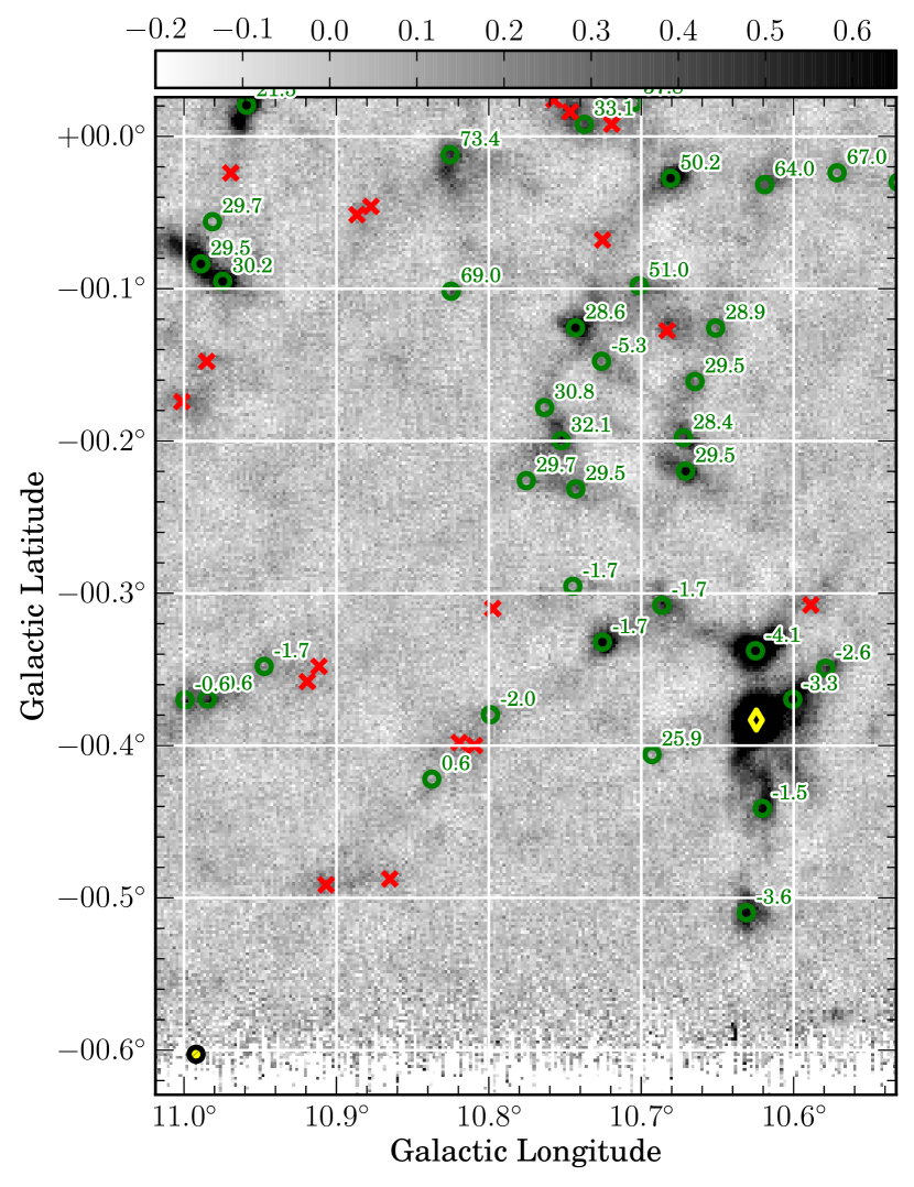
Figure 7: Example finder chart for the $0.5$^∘ region centered on $l=10.5$^∘ $b=-0.3$^∘. Velocities of BGPS clumps (km/s) overlaid on the BGPS 1.1 mm v2.0 continuum image. Green circles indicate a single $v_{LSR}$ component detection, yellow diamonds indicate multiple $v_{LSR}$ detected, and rojo crosses indicate no HCO⁺ or N₂H⁺ $3-2$ detection. The grey scale is flux density in units of Jy. The Bolocam beam at 1.1 mm is shown as the filled yellow circle in the lower left.

Many BPGS sources appear to be physically associated with complexes of sources. This is evident in the kinematic finder chart centered on $l=10.75$^∘, $b=-0.3$^∘ (Figure 7). The BGPS v2.0 1.1 mm continuum images is displayed in greyscale with flux density indicated along the top. Sources with unique velocity detections are displayed as green circles with the $v_{LSR}$ indicated above the source. Red crosses correspond to positions with no detection. Yellow diamonds correspond to sources with multiple velocity components. The brightest 1.1 mm complex in the southwest quadrant of Figure 7 ranges in velocity from $-4.1$ to $-1.5$ km/s and appears to be both spatially and kinematically connected. There is a second, weaker 1.1 mm complex to the northeast that ranges in velocity from $+28.6$ to $+30.8$ km/s that may be two vertical (aligned in Galactic latitude) filaments. Two sources at $-5.3$ and $+51.0$ km/s are clearly interlopers and are not associated once $v_{LSR}$ is taken into account. This example highlights the need for kinematic information to determine whether objects might be associated.

A simple tool for analyzing whether sources are kinematically associated is to study the distribution of nearest neighbors to each spectroscopically-detected source. We calculate the difference in velocity, $\Delta v_{LSR}$, for the nearest neighbor for all single component molecular detections. The distribution of $\Delta v_{LSR}$ is shown in Figure 8 for all nearest neighbor sources that are within $10$′ (1516 sources). Just over 2/3 of nearest neighbors appear kinematically associated ($69$% of nearest neighbors have $\Delta v_{LSR}<7$ km/s). This is not a surprising result because multiple BGPS clumps may lie within the same molecular cloud traced by CO (e.g. Eden et al. 2012, 2013). Identifying physically connected clumps or filaments is difficult in the BGPS maps because of the spatial filtering due to atmospheric subtraction; however, observations from the Herschel Space Observatory will suffer less severe spatial filtering than ground-based observations. Early Herschel observations revealed a plethora of filaments within the Galactic plane (e.g., Men’shchikov 2010, Molinari et al. 2010, Arzoumanian et al. 2011, Palmeirim et al. 2012) The kinematic information presented in this paper will be crucial for finding spatially and kinematically connected filaments in observations of the Galactic plane from the Herschel Space Observatory.

4.1.1 A Methodology for Deriving Heliocentric Distances

Ultimately, in order to derive physical properties of BGPS clumps such as size, mass, and luminosity, we must determine the heliocentric distances, $d_{\odot}$. For sources in the first quadrant, resolving the kinematic distance ambiguity (KDA) presents a formidable problem. The top left panel of Figure 8 shows the distribution of the difference between the far and near heliocentric distance. The majority of sources observed in the first quadrant have $\Delta d_{\odot}=d_{\rm{far}}-d_{\rm{near}}$ that vary between $3-10$ kpc. For physical quantities, such as the mass or the luminosity, that functionally depend on $d_{\odot}^{2}$, the resulting uncertainty are factors of one to two orders of magnitude.

It is unlikely that we will be able to uniquely resolve the KDA for every spectroscopic detection in this catalog. A statistical approach is more appropriate to characterize the probability of finding a source at a given distance. The companion paper to this survey by Ellsworth-Bowers et al. (2013) develops a Bayesian technique for deriving the posterior Distance Probability Density Functions (DPDF) for BGPS clumps. In this framework, the posterior distribution is given by the product of the likelihood function (derived from $v_{LSR}$ and the rotation curve of the Galaxy) and prior distributions that constrain the probability of finding the source at near or far kinematic distances

$$DPDF(d_{\odot})=\mathcal{L}(v_{LSR},l,b;d_{\odot})\,\prod_{i}P_{i}(d_{\odot},l,b)\;\;.$$ (1)

The likelihood function, $\mathcal{L}(v_{LSR},l,b;d_{\odot})$, is a bimodal distribution with equal probability centered on the near and far kinematic distances derived from the Reid et al. (2009) rotation model of the Galaxy with a $7$ km/s uncertainty (see Ellsworth-Bowers et al. 2012, Reid et al. 2009). Ellsworth-Bowers et al. (2013) develops two prior distributions based on the azimuthally averaged distribution of H₂ in the Galaxy (Wolfire et al. 2003) and a radiative transfer model of the Galactic 8 $\mu$m emission (Robitaille et al. 2012) to derive the DPDF for BGPS sources associated with 8 $\mu$m absorption features (EMAFs) observed in Spitzer images. This study shows that not all EMAFs can be automatically associated with the near kinematic distance; 15% of BGPS sources associated with EMAFs are placed at or beyond the tangent distance. Additional prior distributions (i.e. based on the presence or lack of HI absorption features; see Roman-Duval et al. 2009) may be used to further constrain the DPDFs. The distribution of a source property (i.e. size, mass, luminosity, etc.) may then be calculated using Monte Carlo techniques that marginalize over distance (randomly drawn from the DPDFs) and other relevant physical variables (i.e. dust temperature and dust opacity in the calculation of mass from the observed 1.1 mm flux; see Schlingman et al 2011). Calculation of DPDFs for the entire spectroscopic catalog is beyond the scope of this current paper and is the subject of ongoing work by the BGPS team.

There is no distance ambiguity for Galactocentric radius, $R_{gal}$. This permits us to compare the molecular derived properties vs. $R_{gal}$ for the subset of 3126 unique kinematic detections. The Galactocentric radius may be derived from the observed $v_{LSR}$, $l$, $b$, and the assumed rotation curve of the Galaxy ($v(r)$). We use the Reid et al. (2009) model for the rotation curve of the Milky Way determined from parallax measurements of maser sources. A FORTRAN program supplied by M. Reid (2009; private communication) calculates the near or far kinematic distances from observed $v_{LSR}$ and galactic coordinates. The bottom panel of Figure 8 shows the distribution of sources with $R_{gal}$. Four distinct peaks are visible: the molecular ring at $4.5$ kpc, the Sagittarius arm at $6.5$ kpc, the Local arm at $8.5$ kpc, and the outer Perseus arm at $10.5$ kpc.

4.2 Molecular Intensity Comparisons

The brightest HCO⁺ $3-2$ sources have integrated intensities over 150 K km/s. The brightest HCO⁺ $3-2$ source, (6362 G49.489-0.370) is also the brightest 1.1 mm source and appears associated with the luminous infrared source W51 IRS2S (Wynn-Williams, Becklin, & Neugebauer 1974). Both the HCO⁺ and N₂H⁺ $3-2$ spectra display a strong red asymmetry likely indicative of the strong molecular outflows in this region. The brightest N₂H⁺ $3-2$ source is 2152 (G015.013-00.674) with $I=42.6$ K km/s and is associated with the M17-SW region.

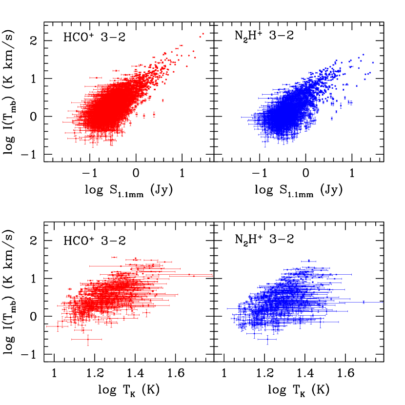
Figure 9: The integrated intensity of HCO⁺ $3-2$ (top left) and N₂H⁺ $3-2$ (top right) vs. $1.1$ mm flux density from v2.0 maps. The integrated intensity of HCO⁺ $3-2$ (bottom left) and N₂H⁺ $3-2$ (bottom right) vs. gas kinetic temperature determined from NH₃ observations.

Schlingman et al. (2011) reported a correlation between the HCO⁺ and N₂H⁺ $3-2$ integrated intensities and the 1.1m flux density for the subset of 1882 sources observed. The correlations for the complete spectroscopic catalog are plotted in Figure 9. Similar positive correlations are observed for both molecules (Pearson’s product-moment correlation coefficient is $r_{corr}=0.78$ for HCO⁺ $3-2$ and $r_{corr}=0.75$ for N₂H⁺ $3-2$). The excellent overlap in points between new observations presented in this paper the Schlingman catalog indicates that the calibration between the two sets of observations is consistent (§2).

The bottom panels of Figure 9 also show a correlation between HCO⁺ integrated intensity and kinetic temperature indicating that warmer sources have more HCO⁺ $3-2$ emission ($r_{corr}=0.62$). N₂H⁺ $3-2$ emission is slightly less well correlated with $T_{k}$ ($r_{corr}=0.53$). There is, however, a tendency for N₂H⁺ $3-2$ emission to be brighter in warmer clumps. This is likely due to excitation conditions in those clumps. The $J=3$ level is $26.8$ K above ground and the level populations and subsequent intensity of the $3-2$ line are sensitive to the gas kinetic temperature (see §4.4). It will be important to ultimately compare the $1-0$ transitions, for instance from the MALT90 survey (Foster et al. 2011, 2013), to derive the chemical abundances of HCO⁺ and N₂H⁺ with less sensitivity to excitation conditions.

We also find positive correlations in the integrated intensities of HCO⁺ and N₂H⁺ $3-2$ emission ($r_{corr}=0.82$) and in the ratio $I_{\rm{line}}/S_{1.1}$ ($r_{corr}=0.62$; Figure 9). This ratio of integrated intensity to 1.1 mm flux density is linearly proportional to the molecular abundance if molecular emission is in the optically thin limit. We must caution that the assumption that HCO⁺ and N₂H⁺ $3-2$ emission is optically thin is likely untrue for most BGPS sources and that optical depth effects will modify optically-thin column densities by the factor $\frac{\tau}{1-exp(-\tau)}\sim\tau$ for thick lines (see §4.4).

HCO⁺ and N₂H⁺ have opposite chemical behavior with respect to CO. HCO⁺ is primarily formed in the gas phase from reactions of CO with H${}_{3}^{+}$ while N₂H⁺ is destroyed by gas phase CO (see Jørgensen et al. 2004). Since CO is adsorbed onto dust grains at high densities ($n>10^{4}$ cm³) and low temperatures ($T_{k}<20$ K), the gas phase abundances of HCO⁺ and N₂H⁺ are expected to be anti-correlated in cold, dense, heavily CO-depleted environments. The correlations observed above seem to contradict the simple chemical expectation if they are naively interpreted as representing variations in the abundance of HCO⁺ and N₂H⁺. However, we must be careful when directly comparing integrated intensities since this quantity is function of both the column density (or abundance) and the excitation conditions, which play an important role for the $3-2$ transitions (see §4.4).

A large ratio of N₂H⁺/HCO⁺ emission may be a better indicator of a significant reservoir of cold, dense gas within a BGPS clump. There are 113 sources (1.8%) with brighter N₂H⁺ $3-2$ integrated intensities than HCO⁺ $3-2$ lines. In contrast, the CHaMP survey (Census of High- and Medium-mass Protostars; Barnes et al. 2010, 2011) does not find any high-mass clumps in the their follow-up mapping survey of 303 sources in the fourth quadrant with N₂H⁺ $1-0$ integrated intensities larger than HCO⁺ $1-0$ intensities (see Figure 3 of Barnes et al. 2013). Mapping observations of HCO⁺ $3-2$ and N₂H⁺ $3-2$ toward IRDCs with BGPS clumps have revealed significant chemical differentiation of these two species on clump scales (see Battersby et al. 2010). Our survey indicates that, while rare, N₂H⁺-brighter sources do occur.

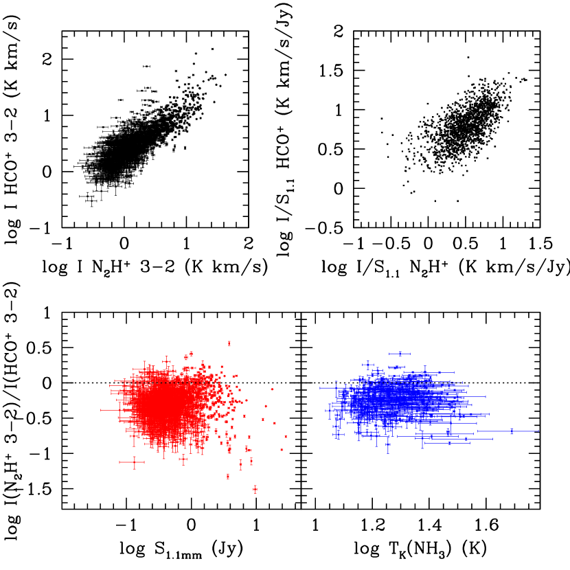
Figure 10: TOP LEFT: A strong correlation is observed between the HCO⁺ and N₂H⁺ $3-2$ integrated intensities. TOP RIGHT: A weaker correlation is observed between HCO⁺ and N₂H⁺ $3-2$ integrated intensity to 1.1 mm flux density ratio. Errorbars have been suppressed to better display the points. BOTTOM LEFT: The integrated intensity ratio N₂H⁺ / HCO⁺ $3-2$ vs. $1.1$ mm flux density from v2.0 maps. BOTTOM RIGHT: The integrated intensity ratio N₂H⁺ / HCO⁺ $3-2$ vs. gas kinetic temperature determined from NH₃ observations.

Schlingman et al. (2011) explored the N₂H⁺/HCO⁺ $3-2$ ratio toward the subset of 1882 sources observed and found a lack of correlation in the molecular intensity ratio and 1.1 mm flux density. The complete set of observations confirms this lack of correlation ($r_{corr}=0.02$; Figure 10). We also observe a lack of correlation in the molecular ratio compared to the gas kinetic temperature measured using NH₃ observations ($r_{corr}=0.01$; Figure 10). At $30$″ resolution, the 1.1 mm continuum, HHT, and GBT spectroscopic observations probe a spatial extent of $0.73$ pc $(D/5\,\rm{kpc})$. This is very similar to the median size of BGPS clumps $0.75$ pc found by Schlingman et al. BGPS clumps are very unlikely to be single massive cores (median $M\sim 300$ M_⊙; Schlingman et al. 2011), but are likely to be composed of multiple smaller cores as confirmed by recent higher angular resolution observations (Merello et al., in prep.). The lack of a significant correlation in the molecular ratio with 1.1 mm flux suggests that there is variation in the fraction of cold, dense, CO-depleted gas between cores that are in BGPS clumps. This result can also be explained by the multiple core hypothesis if the cores within a BGPS clump have different average gas kinetic temperatures. This hypothesis may be tested with interferometric observations. The 113 sources with an intensity ratio of N₂H⁺/HCO⁺$>1$ are candidates for containing a dense, cold core within the clumps even though the beam-averaged gas kinetic temperature spans a factor of 3.

4.3 Linewidth and Full Width Zero Intensity

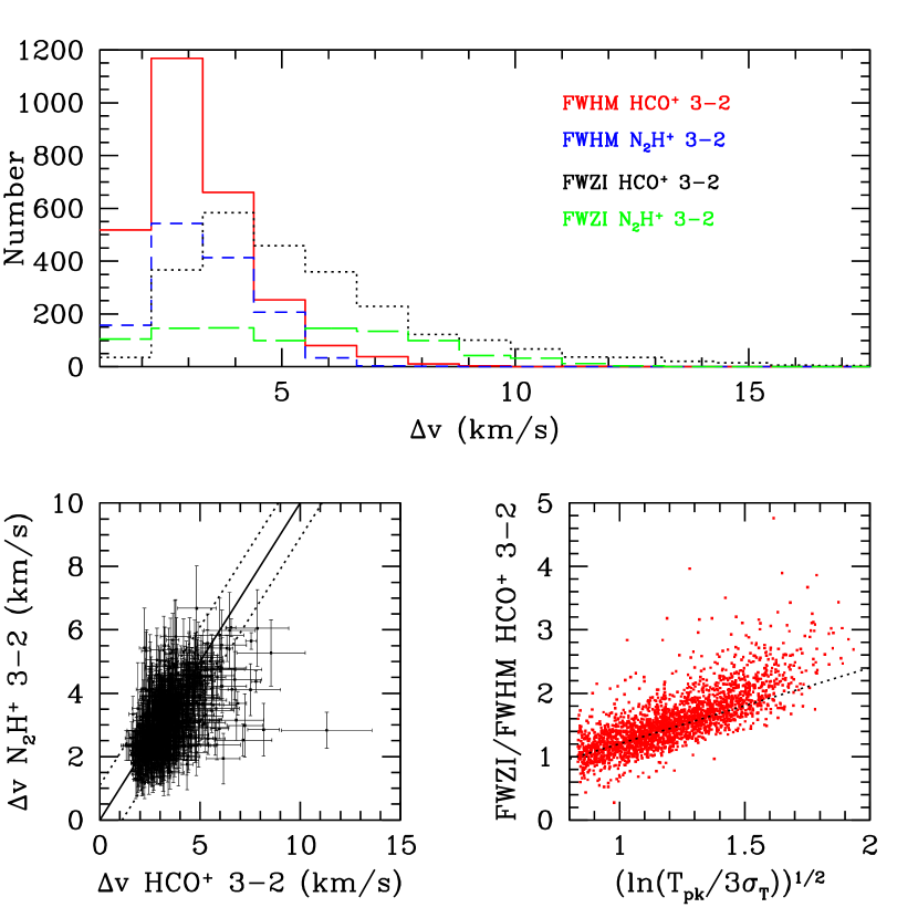
Figure 11: TOP: Histograms of HCO⁺ $3-2$ FWHM (solid red line), N₂H⁺ $3-2$ FWHM (short-dashed blue line), HCO⁺ $3-2$ FWZI (doted black line), and N₂H⁺ $3-2$ FWZI (long-dashed green line). BOTTOM LEFT: A correlation is observed between the N₂H⁺ $3-2$ and HCO⁺ $3-2$ linewidths. A solid 1:1 line is plotted with dashed lines offset by the velocity resolution of one channel (1.1 km/s). BOTTOM RIGHT: The ratio of FWZI/FWHM for HCO⁺ $3-2$ correlates against $\sqrt{\ln(T_{pk}/3\sigma_{T_{mb}})}$. The dashed line shows the expected relationship for a Gaussian line shape.

The distributions of FWHM linewidth, $\Delta v$, for HCO⁺ and N₂H⁺ $3-2$ spectra with a flag $=1$ that are well fit by a Gaussian line shape are shown in Figure 11. These distributions for the full catalog are similar to those found by Schlingman et al. (2011) with a median line width of $3.3$ km/s for both HCO⁺ $3-2$ and for N₂H⁺ $3-2$. Both distributions are positively skewed, showing a small tail that reaches linewidths up to 16 km/s. There are 559 HCO⁺ $3-2$ detections with measured $\Delta v<2.2$ km/s; some of these 559 sources may have smaller $\Delta v$ but we are limited by the velocity resolution (1.1 km/s) of the spectrometer. In comparison, Wienen et al. (2012) find that the observed linewidth of NH₃ (1,1) is $\sim 2$ km/s with very few sources below $1$ km/s (their spectral resolution is a factor of two better than this survey at $0.5$ km/s). The HCO⁺ and N₂H⁺ linewidths observed in this survey are plotted against each other in Figure 11. A few sources have HCO⁺ $3-2$ linewidths that are larger than their corresponding N₂H⁺ $3-2$ linewidth, but most sources cluster around the $1:1$ line.

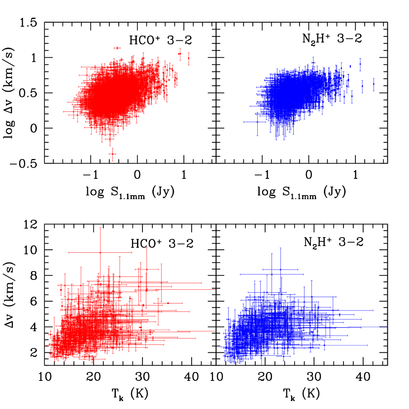
Figure 12: The HCO⁺ $3-2$ FWHM (top left) and the N₂H⁺ $3-2$ FWHM (top right) vs. 1.1 mm flux density. The HCO⁺ $3-2$ FWHM (bottom left) and the N₂H⁺ $3-2$ (bottom right) vs. gas kinetic temperature.

The measured HCO⁺ and N₂H⁺ $3-2$ linewidths are compared to the observed 1.1 flux density and gas kinetic temperatures in Figure 12. None of these plots are well correlated; however, there are some discernible trends. HCO⁺ $3-2$ linewidth has a lower bound that increases with 1.1 mm flux density. For instance, sources with $S_{1.1}>1$ Jy have $\Delta v$(HCO⁺ $3-2)>1.6$ km/s while sources with $S_{1.1}>10$ Jy have $\Delta v$(HCO⁺ $3-2)>5$ km/s. Similarly, there is an increasing lower bound for linewidth with kinetic temperature. All $\Delta v$(HCO⁺ $3-2)<1.5$ km/s have $T_{k}<20$ K while all sources with $T_{k}>23$ K have $\Delta v$(HCO⁺ $3-2)>3$ km/s. The highest flux density and highest gas kinetic temperatures tend to have large ($>$ few km/s) linewidths.

The observed linewidths are typically more than an order of magnitude larger than the expected thermal broadening in the line ($0.17$ km/s $\sqrt{T_{k}/18.3\rm{K}}$). If the non-thermal contribution to the linewidths in the clumps is due to turbulent motions, then the observed values indicate that supersonic turbulence dominates BGPS clumps. Schlingman et al. (2011) showed that the standard supersonic turbulence scaling relationships for molecular clouds measured in CO (Larson’s Law; Larson 1981) de-correlates in the dense gas tracers. This may be due to dissipation of turbulence in the denser molecular gas; however, the observed linewidths are not systematically smaller than the predicted relationship for sizes below 1 pc from Larson’s Law determined from CO clouds (see Schlingman et al. 2011). Alternatively, re-injection of turbulence by star-formation likely occurs within a subset of the clumps (Murray et al. 2011). Higher flux density sources and warmer sources are more likely to harbor embedded protostars (see Dunham et al. 2011b) whose winds and outflows may contribute to the turbulent gas motions within the BGPS clump.

Assigning the entire observed linewidth to turbulence is difficult though since unresolved bulk flows in the gas may also contribute to $\Delta v$. In nearby molecular clouds, velocity gradients of $1$ km/s/kpc have been measured as well as inflowing motions along filaments (e.g. Kirk et al. 2013). Examples of bulk flows may be seen in the HCO⁺ $3-2$ spectra from this survey which display a self-absorbed blue asymmetry (see §4.5). Optical depth will also increase the linewidth. An optical depth of $\tau=10$ will double the observed linewidth (Philips et al. 1979, Shirley et al. 2003; see §4.4). The observed line width is likely a combination of unresolved bulk motions (gradients or flows), optical depth effects, and supersonic turbulence. Detailed study of the kinematics within BGPS clumps requires the higher spatial resolution currently only possible with interferometers.

We also find a lack of correlation between the N₂H⁺ / HCO⁺ molecular ratio and the observed linewidth. There are BGPS source with a molecular intensity ratio $>1$ and with large $>5$ km/s linewidths. This chemical ratio does not depend on the amount of turbulence in the clump.

The Full Width Zero Intensity (FWZI) of a spectral line is the width of the line at the $3\sigma_{T_{mb}}$ level. While the measured FWZI depends on the rms noise level in the map, it can be determined for any line shape whereas the FWHM is determined from the fit of a Gaussian line shape. We calculate the FWZI for HCO⁺ $3-2$ spectra by finding the velocity of the first spectral channel on each side of the line peak which has a $T_{mb}<3\sigma_{T_{mb}}$. The resulting HCO⁺ FWZI are quantized by the channel spacing ($1.1$ km/s). For low signal-to-noise spectra, the quoted FWZI will be a lower limit to the true value. We only report FWZI for detections with $T_{mb}\geq 6\sigma_{T_{mb}}$ (2471 HCO⁺ $3-2$ detections).

The histogram of FWZI is plotted in Figure 11. The median FWZI for HCO⁺ $3-2$ lines is 4.5 km/s. The distribution has a tail of FWZI out to 32.5 km/s. The largest FWZI corresponds to source 6901 (G081.680+00.540), an outflow associated with the famous DR21 complex (see Davis & Smith 1996). There are 38 sources with FWZI $>15$ km/s. These objects are strong outflow candidates.

For a Gaussian line shape, the FWZI is directly related to the peak signal-to-noise of the spectrum by

$$\frac{FWZI}{\Delta v}=\frac{1}{\sqrt{2}}\sqrt{\ln(T_{pk}/3\sigma_{T})}\;\;\;,$$ (2)

where $\Delta v$ is the FWHM. The ratio of FWZI/FWHM is plotted in Figure 11 for sources with a HCO⁺ flag = $1$ and shows a distinct correlation that generally follows the line predicted for a Gaussian line shape. The upward trend of FWZI/FWHM away from the dashed line in Figure 11 represent sources with non-Gaussian line shapes indicative of asymmetries or line wings in the spectra. However, most sources in the survey have line shapes that are consistent with a Gaussian line shape. We discuss self-absorbed profiles in detail in §4.5.

4.4 Optical Depth and Excitation Temperature

The optical depth in the HCO⁺ $3-2$ line may be determined from observations of an isotopologue and the radiative transfer equation assuming that the excitation temperature of the HCO⁺ and H¹³CO⁺ $3-2$ transitions are identical and that there is no fractionation between the interstellar ratio $[^{13}\rm{C}]/[^{12}\rm{C}]$ the the molecular [H¹³CO⁺]/[HCO⁺] ratio. The peak optical depth of the HCO⁺ $3-2$ transition is determined from the non-linear equation

$$\frac{T_{mb}(\rm{HCO}^{+})}{T_{mb}(\rm{H}^{13}\rm{CO}^{+})}=\frac{1-\exp(-\tau)}{1-\exp(-\tau\frac{[^{13}\rm{C}]}{[^{12}\rm{C}]})}\;\;.$$ (3)

Observations were made during the final shift of observing in December 2012 in the H¹³CO⁺ $3-2$ line ($260.255339$ GHz) toward $48$ v1.0.1 sources in the Gem OB 1 star formation complex ($188$^∘ $<l<193$^∘; see Reipurth & Yan 2008) with HCO⁺ $3-2$ detections. Emission was detected for 34 sources ($71$%). Every source with a H¹³CO⁺ $3-2$ detection has an optically thick HCO⁺ $3-2$ line with the average optical depth for this subset of $\tau=10.2\pm 4.7$ assuming $[^{13}\rm{C}]/[^{12}\rm{C}]=50$ (see Table 5). Sources with H¹³CO⁺ $3-2$ non-detections are generally weak in HCO⁺ $3-2$ resulting in an average $3\sigma$ upper limit of $\tau<20$. It is likely that even these weak HCO⁺ lines are optically thick.

Due to the large optical depth observed we can solve for the excitation temperature in the HCO⁺ $3-2$ line,

$$T_{ex}^{obs}=\frac{h\nu/k}{\ln\left(1+\frac{h\nu/k}{T_{mb}/f+J_{\nu}(T_{cmb})}\right)}\;\;,$$ (4)

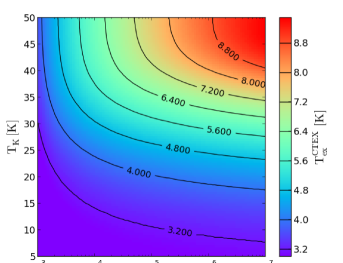
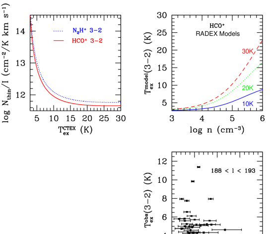
Figure 13: TOP LEFT: Optically thin column density of HCO⁺ $3-2$ (solid red line) and N₂H⁺ $3-2$ (dotted blue line) versus $T_{ex}^{CTEX}$. Below $T_{ex}^{CTEX}=10$ K, the column density becomes a sensitive function of excitation temperature. TOP RIGHT: The model excitation temperature of HCO⁺ $3-2$ versus volume density for constant density, constant kinetic temperature radiative transfer models with $\log N/\Delta v=13.5$ (RADEX; van der Tak et al. 2007). The blue (solid) curves is $T_{k}=10$ K, the green (dotted) curve is $T_{k}=20$ K, and the red (dashed) curve is $T_{k}=30$ K. BOTTOM LEFT: Contours of $T_{ex}^{CTEX}$ for HCO⁺ $3-2$ observations from constant density, constant kinetic temperature models. BOTTOM RIGHT: Peak optical depth of the HCO⁺ $3-2$ line calculated from H¹³CO⁺ $3-2$ observations. HCO⁺ $3-2$ emission is typically optically thick and sub-thermally populated in the physical conditions found in BGPS clumps.

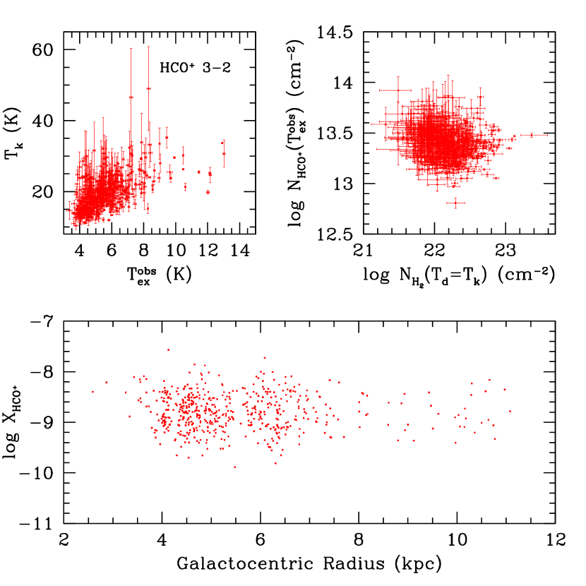
Figure 14: TOP LEFT: The gas kinetic temperature versus the excitation temperature determined from the HCO⁺ $3-2$ line. TOP RIGHT: The column density of HCO⁺ versus the H₂ column density assuming $T_{d}=T_{k}$. Only the subset of sources with NH₃ observations are plotted. BOTTOM: The HCO⁺ $3-2$ abundance does not vary systematically with Galactocentric radius.

where $f$ is the filling fraction of emission and $J_{\nu}(T)=h\nu/k/(\exp(h\nu/kT)-1)$ is the Planck function in temperature units. The observed excitation temperatures are shown in Figure 13, assuming $f=1$, plotted against the observed optical depth for sources associated with Gem OB 1. The average excitation temperature is $T_{ex}^{obs}=5.3\pm 2.0$ K, much lower than typical gas kinetic temperatures observed toward BGPS sources with NH₃ $T_{k}$ determinations (Figure 5). Assuming that HCO⁺ emission is optically thick for all BGPS sources, we can compare the excitation temperature with $T_{k}$ for this subsample. The average $T_{ex}^{obs}=5.5\pm 1.4$ K is very similar to the average found for sources in Gem OB 1. The observed excitation temperatures are weakly correlated with the gas kinetic temperature (Figure 14) with sources that have $T_{ex}^{obs}>8$ K typically having $T_{k}>20$ K.

We compare the observed $T_{ex}^{obs}$ to the excitation of the $3-2$ transition from a single zone radiative transfer model. The top right panel of Figure 13 shows the model excitation temperature for single density, single kinetic temperature models calculated using RADEX (van der Tak et al. 2007). The three curves correspond to gas kinetic temperatures spanning the range of $T_{k}=10$ to $30$ K. For the typical average volume densities probed toward BGPS clumps of $10^{3}-10^{4.5}$ cm^-3 (Schlingman et al. 2011, Dunham et al. 2011), the model excitation temperature is $<7$ K with $T_{ex}^{model}<<T_{k}$. $T_{ex}^{model}$ agrees well with the observed median $T_{ex}^{obs}$ indicating that most of the 3122 HCO⁺ $3-2$ lines observed in this survey are very sub-thermally populated. Unfortunately, it would a prohibitively long survey to determine the optical depth in all 3122 HCO⁺ $3-2$ detections using H¹³CO⁺ $3-2$ observations.

The excitation temperature must be determined or assumed to derive a column density from the observed integrated intensity. In the optically thin, constant excitation temperature limit ($T_{ex}=T_{ex}^{CTEX}\;\forall J$), the total column density derived from the integrated intensity of HCO⁺ and N₂H⁺ $3-2$ emission is given by

$$N_{\rm{thin}}=\frac{8\pi k\nu^{2}f}{7hc^{3}A_{3-2}}\frac{Q(T_{ex})J_{\nu}(T_{ex})e^{E_{u}/kT_{ex}}}{J_{\nu}(T_{ex})-J_{\nu}(T_{cmb})}\int T_{mb}\,dv\;\;,$$ (5)

where $A_{3-2}$ is the Einstein spontaneous emission coefficent ($1.476\times 10^{-3}$ s^-1 for HCO⁺ $3-2$ and $1.259\times 10^{-3}$ s^-1 for N₂H⁺ $3-2$), $Q$ is the partition function and $E_{u}/k$ is the energy of the upper ($J=3$) level ($25.68$ K for HCO⁺ $3-2$ and $26.83$ K for N₂H⁺ $3-2$). For the $3-2$ transitions of both molecules, the column density becomes a sensitive function of $T_{ex}$ below 10 K (Figure 13). The excitation temperature derived from Equation 3 ($T_{ex}^{obs}$) applies only for the $J=3$ level, but the excitation temperature for the CTEX approximation is potentially different because of non-LTE excitation. The bottom left panel of Figure 13 calculates $T_{ex}^{CTEX}$ from Equation 4 for a grid of models with constant density and constant kinetic temperature assuming a total HCO⁺ column density of $3.16\times 10^{13}$ cm^-2 ($logN=13.5$ which is the standard assumption used to calculate $n_{eff}$). The plotted contours span $3.1<T_{ex}^{CTEX}<7$ K for the range of average kinetic temperature measured from NH₃ observations. This range overlaps the $\langle T_{ex}^{obs}\rangle$ calculated from Equation 3 indicating that assuming $T_{ex}^{obs}\approx T_{ex}^{CTEX}$ in Equation 4 is a reasonable approximation for BGPS clumps. Using this approximation, the median HCO⁺ column density is $2.5\times 10^{13}$ cm^-2.

If we assume $5$ K as a typical excitation temperature and assume the filling fraction of emission is $f\approx 1$, the HCO⁺ $3-2$ integrated intensities may be converted to optically thin column densities using the scale factor $N_{\rm{HCO}^{+}}/I_{\rm{HCO}^{+}}=6.9\times 10^{12}$ cm^-2 K^-1 (km s^-1)^-1 and the N₂H⁺ $3-2$ emission scale factor of $N_{\rm{N_{2}H}^{+}}/I_{\rm{N2H}^{+}}=1.0\times 10^{13}$ cm^-2 K^-1 (km s^-1)^-1. The corresponding $3\sigma$ upper limit to the optically thin HCO⁺ $3-2$ column density in this survey is $N_{3\sigma}>1.2\times 10^{12}$ cm^-2. However, we know that the HCO⁺ $3-2$ line is likely optically thick from the results of H¹³CO⁺ $3-2$ observations; therefore, we should apply a correction to the optical depth of $N=N_{thin}\tau/(1-e^{\tau})$ (Goldsmith & Langer 1999). The HCO⁺ column densities shown in Figure 14 are likely lower limits because we do not know the true optical depth for sources outside Gem OB 1.

We plot the HCO⁺ column density versus the total H₂ column density calculated from the 1.1 mm peak flux density assuming Ossenkopf & Henning (OH5) opacities and that the dust temperature is equal to the gas kinetic temperature from NH₃ observations (Figure 14). Gas kinetic temperature and dust temperature are only expected to be well coupled at high densities ($n>10^{5}$ cm^-3; see Goldsmith 2000); however, in the absence of other information, it is a better approximation than assuming all sources are at the same dust temperature. The plotted column density errorbars are purely statistical errors based on the uncertainty in $\sigma_{T_{mb}}$. The total uncertainty in the HCO⁺ column density is dominated by the uncertainty in the unknown filling fraction of emission and the uncertainty in the unknown optical depth which would likely increase the column density by factors of a few. With these caveats in mind, we plot the HCO⁺ column density and abundances in Figure 14. In contrast with the integrated intensity correlation (§4.2), there is no correlation between the HCO⁺ and H₂ column densities. This result again highlights the importance of the excitation conditions and not the total molecular column density in driving the observed intensity correlations. A similar lack of correlation was also observed for NH₃ column densities versus H₂ column densities by Wienen et al. (2012). We find a median HCO⁺ abundance of $1.6\times 10^{-9}$. The HCO⁺ abundance also shows no discernible trend with Galactocentric radius (Figure 14). This result is in contrast with NH₃ observations which show a decrease by a factor of 7 in abundance with Galactocentric radius (Dunham et al. 2011a). Both studies are limited by a paucity of sources at large Galactocentric radius with measured gas kinetic temperatures.

Unfortunately, we cannot easily calculate the optical depth in the N₂H⁺ $3-2$ line because the 45 hyperfine lines are too heavily blended to obtain believable constraints. Furthermore, observations of the ${}^{15}\rm{NNH}^{+}$ isotopologue is prohibitive because the interstellar $[^{15}\rm{N}]/[^{14}\rm{N}]$ abundance is a factor of $5-10$ smaller than the ISM $[^{13}\rm{C}]/[^{12}\rm{C}]$ abundance (Wilson & Rood 1994, Adande & Ziurys 2012). N₂H⁺ $3-2$ is also very likely sub-thermally populated based on our radiative transfer calculations. Given the more than order of magnitude uncertainties, we do not report column densities for N₂H⁺ $3-2$ emission. We recommend observations of the N₂H⁺ $1-0$ line where the hyperfine splitting is more easily resolved (e.g., Pirogov et al. 2003, Pirogov et al. 2007, Reiter et al. 2011a, Barnes et al. 2013).

4.5 Self-absorbed Line Profiles

While most HCO⁺ $3-2$ lines in the survey are believed to have $\tau>1$ based on limited H¹³CO⁺ $3-2$ observations and comparison to radiative transfer models (§4.4), there is a small percentage of sources that display clear line asymmetries indicative of kinematic motions coupled with very optically thick lines. For a HCO⁺ $3-2$ line profile to be classified as self-absorbed, the profile must show two peaks and an absorption dip over the span of at least 3 channels ($3.3$ km/s) with the N₂H⁺ $3-2$ line profile having a single-peak (HCO⁺ flag = $3$ while N₂H⁺ flag = $1$). This situation occurs for $80$ ($1.3$%) sources (Table 5). Self-absorbed line profiles are extremely rare in this survey. This may, in part, be due to the low spectral resolution ($1.1$ km/s) required to cover the full velocity range ($-60$ to $170$ km/s) of sources in the longitude range observed in the first quadrant.

We may classify the self-absorbed sources sources as blue, red, or equal asymmetries by the location of the $v_{lsr}$ maximum. $47$ sources have a clear blue asymmetry while $26$ sources have a clear red asymmetry and $7$ sources have equal height peaks. The blue excess for the subset of sources showing distinct self-absorption is $(N_{B}-N_{R})/N_{SA}=0.57$. These $80$ sources (listed in Table 4) are excellent high-mass, large-scale collapse candidates (see Reiter et al. 2011b) and should be followed up at higher spatial resolution.

5 Conclusions

In this paper, we have presented a complete spectroscopic catalog for all sources in the BGPS v1.0.1 source catalog with $7.5$^∘$\leq l\leq 194$^∘ and characterized the properties of the molecular emission. 3126 sources ($50.5$%) were detected with unique $v_{LSR}$. HCO⁺ $3-2$ is a significantly better kinematic tracer of BGPS clumps than CO isotopologues with contamination from multiple velocity components rare (only $1.3$%). The detection fraction of BGPS v1.0.1 sources is $>50$% for 1.1 mm sources with flux densities $>200$ mJy and $>90$% for flux densities $>500$ mJy. The majority of BGPS clumps appear to be physically associated with other clumps. This is the largest targeted dense gas survey of the Milky Way to date and traces the major spiral arm structures of the Milky Way in Galactocentric radius.

HCO⁺ and N₂H⁺ molecular intensities are well correlated with 1.1 mm flux density and with each other while molecular column densities are not well correlated with the total H₂ column density. HCO⁺ $3-2$ intensity is also correlated with gas kinetic temperature. HCO⁺ $3-2$ emission is likely optically thick and sub-thermally populated ($T_{ex}\sim 5$ K $<<T_{k}$) toward most BPGS clumps. These observed intensity correlations are most likely due to the sensitivity of the $3-2$ transitions to excitation conditions probed by the dense gas. The molecular intensity ratio does not correlate with 1.1 mm flux density, $T_{k}$, or $\Delta v$. BGPS clumps are likely composed of smaller cores which may have a range of different chemical and excitation conditions. Sources with large N₂H⁺/HCO⁺ intensity ratios probably contain significant reservoirs of cold, dense gas. The median $\Delta v=3.3$ km/s (FWHM) and is consistent with supersonic turbulence although optical depth and bulk motions within the core are contributors to the linewidth. The observed linewidth does not correlate with 1.1 mm flux density or $T_{k}$ although the lower bound of $\Delta v$ does correlated with both quantities.

In the coming months, source catalogs from the ATLASGAL and Hi-Gal continuum surveys of the Galaxy will be released. The kinematic data provided in this paper provides the necessary information for calculating kinematic distances. Future work by the BGPS team will use this spectroscopic catalog and expand the priors to better constrain Distance Probability Density Functions and statistically analyze the physical properties of BGPS clumps in different evolutionary stages and in different Galactic environments.

Figure 8: TOP LEFT: The distribution of the difference between the far and near kinematic distances. TOP RIGHT: The distributions of nearest neighbor sources in $\Delta v_{LSR}$ for neighbors that are within $10$′. BOTTOM: The distribution of sources in Galactocentric radius. Peaks are clearly distinguished for the molecular ring, Sagittarius arm, local spur, and Perseus arm.

Table 1: Calibration Efficiencies

MJD Range	$\eta_{LSB}^{Vpol}$	$\eta_{LSB}^{Hpol}$	$\eta_{USB}^{Vpol}$	$\eta_{USB}^{Hpol}$	Catalog
54863 - 54916	0.81 (0.04)	0.70 (0.03)	0.81 (0.03)	0.70 (0.04)	1
54917 - 54919	0.64 (0.01)	0.64 (0.01)	0.64 (0.02)	0.64 (0.02)	1
54920 - 54997	0.81 (0.04)	0.70 (0.03)	0.81 (0.03)	0.70 (0.04)	1
55620 - 55669	0.66 (0.03)	0.56 (0.03)	0.71 (0.03)	0.62 (0.03)	2
55678 - 56216	0.83 (0.03)	0.75 (0.03)	0.82 (0.03)	0.78 (0.03)	2

Table 2: HCO⁺ $3-2$ Observed Properties

Number	Source	$\alpha$(J2000.0)	$\delta$	Catalog	Flag	$v_{LSR}$	$T_{mb}^{pk}$	$\sigma_{T_{mb}}$	$I(T_{mb})$	$\sigma_{I}$	$\Delta v$	$\sigma_{\Delta v}$	FWZI
		h:m:s	d:m:s			(km/s)	(K)	(K)	(K km/s)	(K km/s)	(km/s)	(km/s)	(km/s)
1307	G007.501+00.001	18:02:30.0	-22:28:07.0	2	0	$\cdots$	$\cdots$	0.095	$\cdots$	$\cdots$	$\cdots$	$\cdots$	$\cdots$
1308	G007.507-00.255	18:03:28.7	-22:35:22.3	2	0	$\cdots$	$\cdots$	0.104	$\cdots$	$\cdots$	$\cdots$	$\cdots$	$\cdots$
1309	G007.509+00.403	18:01:00.4	-22:15:46.3	2	1	7.5	0.450	0.086	1.245	0.288	2.7	0.5	$\cdots$
1310	G007.564-00.042	18:02:47.8	-22:26:05.6	2	0	$\cdots$	$\cdots$	0.070	$\cdots$	$\cdots$	$\cdots$	$\cdots$	$\cdots$
1311	G007.600-00.142	18:03:15.0	-22:27:10.1	2	1	153.3	0.477	0.061	1.384	0.235	3.4	0.4	3.4
1312	G007.622+00.002	18:02:45.3	-22:21:45.8	2	0	$\cdots$	$\cdots$	0.081	$\cdots$	$\cdots$	$\cdots$	$\cdots$	$\cdots$
1313	G007.622-00.000	18:02:45.8	-22:21:49.4	2	0	$\cdots$	$\cdots$	0.080	$\cdots$	$\cdots$	$\cdots$	$\cdots$	$\cdots$
1314	G007.632-00.110	18:03:11.9	-22:24:33.1	2	1	153.9	2.254	0.066	13.348	0.290	6.2	0.2	11.2
1315	G007.636-00.150	18:03:21.4	-22:25:31.4	2	1	154.8	0.519	0.060	1.412	0.200	2.7	0.3	3.4
1316	G007.636-00.194	18:03:31.4	-22:26:49.4	2	1	152.6	1.167	0.055	6.192	0.248	5.5	0.2	10.1

Table 3: N₂H⁺ $3-2$ Observed Properties

Number	Source	Catalog	Flag	$v_{LSR}$	$T_{mb}^{pk}$	$\sigma_{T_{mb}}$	$I(T_{mb})$	$\sigma_{I}$	$\Delta v$	$\sigma_{\Delta v}$	FWZI
				(km/s)	(K)	(K)	(K km/s)	(K km/s)	(km/s)	(km/s)	(km/s)
1307	G007.501+00.001	2	0	$\cdots$	$\cdots$	0.113	$\cdots$	$\cdots$	$\cdots$	$\cdots$	$\cdots$
1308	G007.507-00.255	2	0	$\cdots$	$\cdots$	0.097	$\cdots$	$\cdots$	$\cdots$	$\cdots$	$\cdots$
1309	G007.509+00.403	2	0	$\cdots$	$\cdots$	0.093	$\cdots$	$\cdots$	$\cdots$	$\cdots$	$\cdots$
1310	G007.564-00.042	2	0	$\cdots$	$\cdots$	0.078	$\cdots$	$\cdots$	$\cdots$	$\cdots$	$\cdots$
1311	G007.600-00.142	2	1	153.0	0.404	0.082	1.979	0.308	$\cdots$	$\cdots$	$\cdots$
1312	G007.622+00.002	2	0	$\cdots$	$\cdots$	0.067	$\cdots$	$\cdots$	$\cdots$	$\cdots$	$\cdots$
1313	G007.622-00.000	2	0	$\cdots$	$\cdots$	0.078	$\cdots$	$\cdots$	$\cdots$	$\cdots$	$\cdots$
1314	G007.632-00.110	2	1	153.9	1.591	0.079	7.967	0.339	5.3	0.2	8.6
1315	G007.636-00.150	2	1	155.3	0.661	0.068	1.633	0.224	2.5	0.3	4.3
1316	G007.636-00.194	2	1	152.8	0.858	0.086	4.679	0.380	4.9	0.3	6.4

Table 4: HCO⁺ $3-2$ Optical Depth from H¹³CO⁺ 3-2 Observations in Gemini

Number	Source	$T_{mb}$(H13CO+)	$\sigma_{T_{mb}}$	$\tau$(HCO+)	$\sigma_{\tau}$
		(K)	(K)
7460	G188.792+01.027	0.363	0.043	6.61	0.98
7461	G188.948+00.883	1.303	0.035	8.54	0.33
7462	G188.975+00.911	0.208	0.047	10.84	3.32
7463	G188.991+00.859	0.067	0.035	4.23	2.86
7464	G189.015+00.823	0.225	0.040	12.64	3.16
7465	G189.030+00.781	1.273	0.048	11.81	0.60
7471	G189.682+00.185	0.316	0.040	17.44	3.60
7472	G189.713+00.335	0.136	0.040	23.81	14.90
7473	G189.744+00.335	0.110	0.031	8.26	3.16
7474	G189.776+00.343	0.897	0.033	17.13	1.08
7475	G189.782+00.265	0.280	0.044	23.45	6.53
7476	G189.782+00.323	$\cdots$	0.040	$<$ 6.74	$\cdots$
7477	G189.783+00.433	$\cdots$	0.036	$<$ 12.17	$\cdots$
7478	G189.783+00.465	$\cdots$	0.047	$<$ 34.5	$\cdots$
7479	G189.788+00.281	0.102	0.019	9.45	2.75
7480	G189.789+00.291	0.082	0.042	7.03	4.43
7481	G189.804+00.355	0.259	0.038	10.09	1.93
7482	G189.810+00.369	0.137	0.041	6.55	2.43
7483	G189.831+00.343	0.138	0.021	7.73	1.61
7484	G189.834+00.317	0.147	0.041	8.96	3.17
7485	G189.836+00.303	$\cdots$	0.033	$<$ 14.69	$\cdots$
7486	G189.864+00.499	0.095	0.049	3.18	2.18
7487	G189.879+00.319	$\cdots$	0.041	$<$ 24.86	$\cdots$
7488	G189.885+00.319	0.090	0.017	12.71	4.55
7489	G189.888+00.303	0.118	0.035	11.26	4.56
7490	G189.921+00.331	$\cdots$	0.041	$<$ 8.11	$\cdots$
7491	G189.950+00.231	0.104	0.045	5.67	3.00
7492	G189.951+00.331	0.382	0.042	16.68	2.71
7493	G189.990+00.353	$\cdots$	0.048	$<$ 50.30	$\cdots$
7494	G190.006+00.361	0.140	0.041	22.16	11.79
7495	G190.044+00.543	$\cdots$	0.045	$<$ 21.24	$\cdots$
7497	G190.063+00.679	$\cdots$	0.043	$<$ 37.16	$\cdots$
7498	G190.171+00.733	0.289	0.042	15.45	3.56
7499	G190.192+00.719	0.087	0.040	13.12	9.33
7500	G190.240+00.911	0.076	0.023	7.67	3.22
7501	G192.581-00.043	0.790	0.042	9.22	0.64
7502	G192.596-00.051	0.260	0.042	4.34	0.86
7503	G192.602-00.143	$\cdots$	0.045	$<$ 18.08	$\cdots$
7505	G192.629-00.157	0.144	0.040	14.07	5.69
7506	G192.644+00.003	0.074	0.043	4.64	3.32
7507	G192.662-00.083	$\cdots$	0.038	$<$ 20.80	$\cdots$
7508	G192.719+00.043	$\cdots$	0.048	$<$ 9.60	$\cdots$
7509	G192.764+00.101	0.160	0.050	5.63	2.08
7510	G192.816+00.127	$\cdots$	0.022	$<$ 5.73	$\cdots$
7511	G192.968+00.093	$\cdots$	0.051	$<$ 10.03	$\cdots$
7512	G192.981+00.149	0.250	0.043	6.66	1.40
7513	G192.985+00.177	0.145	0.052	5.72	2.43
7514	G193.006+00.115	0.268	0.050	8.66	2.00

Table 5: HCO⁺ $3-2$ Line Asymmetries

Number	Source	Catalog	HCO+ Flag	N2H+ Flag	Asymmetry
1363	G008.458-00.224	2	3	1	b
1377	G008.670-00.356	2	3	1	b
1398	G008.872-00.318	2	3	1	r
1412	G009.212-00.202	2	3	1	b
1421	G009.620+00.194	2	3	1	r
1466	G010.214-00.324	1	3	3	b
1491	G010.416-00.030	2	3	0	b
1518	G010.681-00.028	1	3	1	b
1521	G010.693-00.404	1	3	0	b
1584	G011.083-00.536	1	3	1	b
1659	G011.947-00.036	1	3	1	r
1780	G012.809-00.200	1	3	1	r
1796	G012.861-00.272	1	3	1	r
1803	G012.889+00.490	1	3	1	b
1833	G012.999-00.358	1	3	1	r
1869	G013.211-00.142	1	3	1	r
1943	G013.816+00.003	2	3	0	b
1956	G013.882-00.143	2	3	1	b
2019	G014.244-00.071	1	3	1	e

References

- Adande & Ziurys (2012) Adande, G. R., & Ziurys, L. M. 2012, ApJ, 744, 194
- Aguirre et al. (2011) Aguirre, J. E., Ginsburg, A. G., Dunham, M. K., et al. 2011, ApJS, 192, 4
- Arzoumanian et al. (2011) Arzoumanian, D., André, P., Didelon, P., et al. 2011, A&A, 529, L6
- Barnes (2010) Barnes, P. 2010, From Stars to Galaxies: Connecting our Understanding of Star and Galaxy Formation,
- Barnes et al. (2011) Barnes, P. J., Yonekura, Y., Fukui, Y., et al. 2011, ApJS, 196, 12
- Barnes et al. (2013) Barnes, P. J., Ryder, S. D., O’Dougherty, S. N., et al. 2013, MNRAS, 432, 2231
- Battersby et al. (2010) Battersby, C., Bally, J., Jackson, J. M., et al. 2010, ApJ, 721, 222
- Beuther et al. (2012) Beuther, H., Tackenberg, J., Linz, H., et al. 2012, ApJ, 747, 43
- Contreras et al. (2013) Contreras, Y., Schuller, F., Urquhart, J. S., et al. 2013, A&A, 549, A45
- Dame et al. (2001) Dame, T. M., Hartmann, D., & Thaddeus, P. 2001, ApJ, 547, 792
- Dame & Thaddeus (2011) Dame, T. M., & Thaddeus, P. 2011, ApJ, 734, L24
- Davis & Smith (1996) Davis, C. J., & Smith, M. D. 1996, A&A, 310, 961
- Dunham et al. (2011) Dunham, M. K., Rosolowsky, E., Evans, N. J., II, Cyganowski, C., & Urquhart, J. S. 2011, ApJ, 741, 110
- Dunham et al. (2011) Dunham, M. K., Robitaille, T. P., Evans, N. J., II, et al. 2011, ApJ, 731, 90
- Eden et al. (2012) Eden, D. J., Moore, T. J. T., Plume, R., & Morgan, L. K. 2012, MNRAS, 422, 3178
- Eden et al. (2013) Eden, D. J., Moore, T. J. T., Morgan, L. K., Thompson, M. A., & Urquhart, J. S. 2013, MNRAS, 431, 1587
- Elia et al. (2013) Elia, D., Molinari, S., Fukui, Y., et al. 2013, arXiv:1304.7358
- Ellsworth-Bowers et al. (2013) Ellsworth-Bowers, T. P., Glenn, J., Rosolowsky, E., et al. 2013, ApJ, 770, 39
- Encrenaz & Moreno (2002) Encrenaz, T., & Moreno, R. 2002, Experimental Cosmology at Millimetre Wavelengths, 616, 330
- Evans (1999) Evans, N. J., II 1999, ARA&A, 37, 311
- Foster et al. (2011) Foster, J. B., Jackson, J. M., Barnes, P. J., et al. 2011, ApJS, 197, 25
- Foster et al. (2013) Foster, J. B., Rathborne, J. M., Sanhueza, P., et al. 2013, arXiv:1306.0560
- Ginsburg et al. (2013) Ginsburg, A., Glenn, J., Rosolowsky, E., et al. 2013, arXiv:1305.6622
- Goldsmith & Langer (1999) Goldsmith, P. F., & Langer, W. D. 1999, ApJ, 517, 209
- Hennebelle & Falgarone (2012) Hennebelle, P., & Falgarone, E. 2012, A&A Rev., 20, 55
- Ho & Townes (1983) Ho, P. T. P., & Townes, C. H. 1983, ARA&A, 21, 239
- Jackson et al. (2006) Jackson, J. M., Rathborne, J. M., Shah, R. Y., et al. 2006, ApJS, 163, 145
- Jørgensen et al. (2004) Jørgensen, J. K., Schöier, F. L., & van Dishoeck, E. F. 2004, A&A, 416, 603
- Larson (1981) Larson, R. B. 1981, MNRAS, 194, 809
- Men’shchikov et al. (2010) Men’shchikov, A., André, P., Didelon, P., et al. 2010, A&A, 518, L103
- Molinari et al. (2010) Molinari, S., Swinyard, B., Bally, J., et al. 2010, PASP, 122, 314
- Molinari et al. (2010) Molinari, S., Swinyard, B., Bally, J., et al. 2010, A&A, 518, L100
- Murray (2011) Murray, N. 2011, ApJ, 729, 133
- Ossenkopf & Henning (1994) Ossenkopf, V., & Henning, T. 1994, A&A, 291, 943
- Palmeirim et al. (2013) Palmeirim, P., André, P., Kirk, J., et al. 2013, A&A, 550, A38
- Penzias & Burrus (1973) Penzias, A. A., & Burrus, C. A. 1973, ARA&A, 11, 51
- Phillips et al. (1979) Phillips, T. G., Huggins, P. J., Wannier, P. G., & Scoville, N. Z. 1979, ApJ, 231, 720
- Pirogov et al. (2007) Pirogov, L., Zinchenko, I., Caselli, P., & Johansson, L. E. B. 2007, A&A, 461, 523
- Pirogov et al. (2003) Pirogov, L., Zinchenko, I., Caselli, P., Johansson, L. E. B., & Myers, P. C. 2003, A&A, 405, 639
- Reid et al. (2009) Reid, M. J., Menten, K. M., Zheng, X. W., et al. 2009, ApJ, 700, 137
- Reipurth & Schneider (2008) Reipurth, B., & Schneider, N. 2008, Handbook of Star Forming Regions, Volume I, 36
- Reipurth & Yan (2008) Reipurth, B., & Yan, C.-H. 2008, Handbook of Star Forming Regions, Volume I, 869
- Reiter et al. (2011) Reiter, M., Shirley, Y. L., Wu, J., et al. 2011, ApJS, 195, 1
- Reiter et al. (2011) Reiter, M., Shirley, Y. L., Wu, J., et al. 2011, ApJ, 740, 40
- Robitaille et al. (2012) Robitaille, T. P., Churchwell, E., Benjamin, R. A., et al. 2012, A&A, 545, A39
- Roman-Duval et al. (2009) Roman-Duval, J., Jackson, J. M., Heyer, M., et al. 2009, ApJ, 699, 1153
- Rosolowsky et al. (2010) Rosolowsky, E., Dunham, M. K., Ginsburg, A., et al. 2010, ApJS, 188, 123
- Salpeter (1955) Salpeter, E. E. 1955, ApJ, 121, 161
- Scalo (1986) Scalo, J. M. 1986, Fund. Cosmic Phys., 11, 1
- Schlingman et al. (2011) Schlingman, W. M., Shirley, Y. L., Schenk, D. E., et al. 2011, ApJS, 195, 14
- Shirley et al. (2003) Shirley, Y. L., Evans, N. J., II, Young, K. E., Knez, C., & Jaffe, D. T. 2003, ApJS, 149, 375
- van der Tak et al. (2007) van der Tak, F. F. S., Black, J. H., Schöier, F. L., Jansen, D. J., & van Dishoeck, E. F. 2007, A&A, 468, 627
- Weiland et al. (2011) Weiland, J. L., Odegard, N., Hill, R. S., et al. 2011, ApJS, 192, 19
- Wienen et al. (2012) Wienen, M., Wyrowski, F., Schuller, F., et al. 2012, A&A, 544, A146
- Wilson & Rood (1994) Wilson, T. L., & Rood, R. 1994, ARA&A, 32, 191
- Wolfire et al. (2003) Wolfire, M. G., McKee, C. F., Hollenbach, D., & Tielens, A. G. G. M. 2003, ApJ, 587, 278
- Wynn-Williams et al. (1974) Wynn-Williams, C. G., Becklin, E. E., & Neugebauer, G. 1974, ApJ, 187, 473