Size of discs formed by wind accretion in binaries can be underestimated if the role of wind-driving force is ignored

Abstract

Binary systems consisting of a secondary accreting form a wind-emitting primary are ubiquitous in astrophysics. The phenomenology of such Bondi-Hoyle-Lyttleton (BHL) accretors is particularly rich when an accretion disc forms around the secondary. The outer radius of such discs is commonly estimated from the net angular momentum produced by a density variation of material across the BHL or Bondi accretion cylinder, the latter is tilted with respect to the direction to the primary due to orbital motion. But this approach has ignored the fact that the wind experiences an outward driving force that the secondary does not. In actuality, the accretion stream falls toward a retarded point in the secondary’s orbit as the secondary is pulled toward the primary relative to the stream. The result is a finite separation or “accretion stream impact parameter” (ASIP) separating the secondary and stream. When the orbital radius $a_{o}$ exceeds the BHL radius $r_{b}$, the ratio of outer disc radius estimated as the ASIP to the conventional estimate $a_{o}^{1/2}/r_{b}^{1/2}>1$. We therefore predict that discs will form at larger radii from the secondary than traditional estimates. This agrees with the importance of the ASIP emphasized by Huarte-Espinosa et al. and the practical consequence that resolving the initial outer radius of such an accretion disc in numerical simulations can be less demanding than what earlier estimates would suggest.

1 Introduction

Accretion discs in binary systems play a fundamental role in the phenomenology of high energy emission from compact objects (for reviews see Abramowicz & Straub 2013; Abramowicz & Fragile 2013; Frank, King, Raine 2002). The compact objects can be black holes, neutron stars, or white dwarfs and so the diversity of accretion in binary systems represents evolved states of both low mass and high mass stars. X-ray binaries and microquasars have long been associated with accretion onto neutron stars and black holes and cataclysmic variables have been associated with accretion in a binary onto white dwarfs. And, most recently it has been realized that the prevalence of asymmetric and bipolar planetary nebulae (e.g. Bujarrabal et al. 2001; Balick & Frank 2002) might also be associated with binaries (e.g. De Marco & Soker 2009), and the production of jets from the associated accretion discs (Reyes-Ruiz & Lopez 1999; Soker & Rappaport 2000,2001; Blackman et al. 2001; Nordhaus & Blackman 2006; Witt et al. 2009).

If a binary separation is too large for Roche overflow (e.g. Eggleton 1983; D’Souza et al. 2006) or tidal shredding, a disc may still form around the secondary by the accretion of wind material ejected by the primary. Modeling this mode of accretion disc requires generalizing the so-called Bondi-Hoyle-Lyttleton (BHL) flows (see Edgar 2004 for a review) to include the additional asymmetric effects that arise from orbital motion between the wind emitting primary and the secondary (Shapiro & Lightman 1976; Wang 1981).

The original (and simplest) form of the BHL problem occurs when a compact object of mass, $M_{2}$, moves at a constant supersonic velocity $v_{rel}$ relative to the ambient material though a homogenous plasma cloud. The gravitational field of $M_{2}$ focuses the material located within the “Bondi cylinder” of radius

$$r_{b}=2GM_{2}/v_{rel}^{2},$$ (1)

that extends past the object forming a downstream wake. Downstream, along the Bondi cylinder axis, a stagnation point separates material accreted onto the object from material that flows away and escapes (Bondi & Hoyle, 1944). A conical shock forms downstream around the axis and along this axis the “accretion line” (or ”accretion stream”) connects the stagnation point and the object.

In addition to phenomenological applications of this mode of accretion in binary systems (e.g. Soker & Rapporport 2000; Struck et al. 2004; Perets & Kenyon 2012), there have been a handful of numerical simulations demonstrating the mechanism (Smooth particle Hydrodynamics: Theuns & Jorissen 1993; Mastrodemos & Morris 1998,1999; Grid based: Nagae et al 2004; Jahanara et al. 2005; 2-D Adaptive Mesh: de Val-Boro et al. 2009; 3-D Adaptive Mesh: Huarte-Espinosa et al. 2013). Note also that there have been many more simulations of the basic BHL mechanism without the consideration of the angular momentum Foglizzo, Galletti, & Ruffert2005 .

Huarte-Espinosa et al. (2013), carried out the highest resolution simulations of BHL wind accretion in a binary system in the limit that the orbital speed is less than the wind speed, and that the Bondi radius is less than the orbital scale. There remains opportunity to study a more comprehensive range of companion masses and orbital radii but an important issue for both conceptual understanding of disc formation and for practical considerations in setting up simulations is the minimum scale to resolve. Huarte-Espinosa et al. (2013) deemed that the minimum scale to assess the presence or absence of disc is the accretion stream impact parameter (hereafter ASIP) $b$. This is the distance of closest approach of the BHL accretion stream to the secondary. It is determined by the displacement of the secondary towards the primary over a Bondi accretion time as measured in an inertial frame where the secondary starts from rest and is accelerated towards the primary. This appears essentially like free-fall towards the slowly moving primary. In the limited cases studied, the simulations were consistent with this being the relevant minimum scale scale needed. However, Huarte-Espinosa et al. (2013) did not compare this radius to that of standard estimates of the outer disc radius (e.g. Shapiro and Lightman 1976; Wang et al. 1981) based on the different physics associated with accretion from a density gradient across the Bondi cylinder.

In the present paper, we compare the analytic derivations, physics, and distinct predictions of these two estimates of the minimum outer accretion disc radius in the limit that the orbit speed is much less than the wind speed and the Bondi radius is much less than then orbit radius. We find that the ASIP does indeed provide the larger scale of the two under the same conditions and thus the associated scalings emerge to dominate those of the previous ”standard” estimates. In section 2, we discuss the derivation of the estimate for the BHL disc formation based on a density gradient and a tilted Bondi cylinder. In section 3 we derive the ASIP prediction for the distance of closest approach of the accretion column and we demonstrate that it provides a less restrictive means for forming disks around secondaries. Finally, conclusions are presented in section 4.

2 Estimating the Disc Radius from Accretion in a Density Gradient

In this section we derive and synthesize previous estimates (Shapiro & Lightman 1976, ; Foglizzo, Galletti, & Ruffert2005, ) of the disc radius around the secondary based on the density variation and tilt of the BHL accretion cylinder. The basic geometry is shown in Fig 1 in the frame of the secondary, assuming a top view of what would be a counter-clockwise orbit in the lab frame. The figure shows increased density of flow lines in the half of the Bondi cylinder where the density is higher.

2.1 Velocities of the problem

Although the dimensions are exaggerated for clarity in our figures, we assume in what follows that the Bondi radius of Eq. (1) satisfies $R_{2}<<r_{b}<<a_{o}$, where $R_{2}$ is the physical radius of the secondary and $a_{o}$ is the orbital separation. If we define $r$ as the radial distance from the primary to an arbitrary point in the rotating frame of the secondary, the relative velocity between the secondary and wind material located at $r$ is given by

$$v_{rel}^{2}(r)=v_{w}^{2}+v_{2}^{2}(r),$$ (2)

where $v_{w}$ is the wind speed, and $v_{2}(r)$ is the contribution to velocity from the orbital motion of the secondary. At $r=a_{o}$ we write

$$v_{rel}^{2}(a_{o})=v_{w}^{2}+v_{2,c}^{2},$$ (3)

where $v_{2,c}=v_{2}(a_{o})$. At $r=a_{o}$ we also define $\tan\alpha\equiv v_{2,c}/v_{w}$ where (as seen in Fig. 1), $\alpha$ is the angle between the direction to the primary and the direction of the wind. In what follows, we assume that $v_{w}>>v_{2,c}$ so that $\alpha$ is a small angle and will keep terms only first order in $\alpha$. Since $r_{b}<<a_{o}$, we also have that deviations from $r=a_{o}$ are also small, and can be treated as lowest order corrections.

The explicit expression for $v_{2c}$ is given by

$$v_{2,c}=R_{2}\Omega=R_{2}\left[G(M_{1}+M_{2})\over a_{o}^{3}\right]^{1/2},$$ (4)

which is the circular orbital speed of $M_{2}$ at displacement $R_{2}>0$ from the center of mass. Here $\Omega$ is the orbital speed and $M_{1}$ is the mass of the primary. Defining $R_{1}$ as the magnitude of the displacement of $M_{1}$ from the center of mass, we can eliminate $R_{2}$ from Eq. (4) by noting that

$$a_{o}=R_{1}+R_{2}=R_{2}(1+M_{2}/M_{1})=R_{2}(1+Q)/Q,$$ (5)

where $Q=M_{1}/M_{2}$. Then from Eq. (4),

$$v_{2,c}={Q\over\sqrt{Q+1}}\left[GM_{2}\over a_{o}\right]^{1/2},$$ (6)

where we have used Eqn. (5).

Eq. (4) defines the relative velocity at $r=a_{o}$, but for $r\neq a_{o}$, Eq. (2) requires the position dependent orbital contribution to the total relative velocity between the wind and the secondary. This is given by

$$v_{2}(r)=\frac{r-R_{1}}{R_{2}}v_{2,c}=\frac{r(1+Q)-a_{o}}{a_{o}Q}v_{2,c},$$ (7)

which reduces to $v_{2,c}$ at $r=a_{o}$. We will now express $v_{2}$ in coordinates of the “Bondi disc”, which we define as the cross section of the Bondi cylinder that intersects the secondary. To do so, we define a coordinate system where the x-axis is perpendicular to the direction of the primary (out the plane in Fig. 1 and though the center of the secondary), and the y-axis is oriented in the ‘almost radial’ direction (for small $\alpha$). The Bondi disc is seen edge-on in Fig. 1 and indicated by the thick diagonal line through the secondary. We can then write

$$r=y\sin\alpha+a_{o},$$ (8)

noting that $y$ can be negative. Then at any point within the “Bondi disc”

$$v_{2}(x,y)\simeq v_{2}(r=y\sin\alpha+a_{o})\simeq\frac{y\sin\alpha+a_{o}-R_{1}}{R_{2}}v_{2,c}=\left(1+\frac{y\sin\alpha}{R_{2}}\right)v_{2,c}=\left[1+\frac{y\sin\alpha(1+Q)}{a_{o}Q}\right]v_{2,c},$$ (9)

where we have used Eqn (5) for the last equality. Note that for $y<0$, and $\sin\alpha>0$ this formula gives $v_{2}<v_{2,c}$ as expected since being in the orbital frame means that closer to the center of mass from the position of the secondary, the tangential velocity for a fixed angular velocity is smaller.

2.2 Deriving the condition for disc formation

The outer boundary of the accretion disc around the secondary is expected to form as long as wind material supplied within the Bondi radius has an angular momentum per unit mass about the secondary equal to or larger than the angular momentum per unit mass of material in Keplerian orbit $j_{2}\equiv(GM_{2}R_{k})^{1/2}$ (where $R_{k}$ denotes the disc outer radius). Also, $R_{k}$ must exceed $R_{p}$, the physical radius of the secondary for the disc to form. These conditions for disc formation can be summarized as

$$R_{p}<R_{k}={j_{a}^{2}\over GM_{2}}<r_{b}.$$ (10)

If we write ${j_{a}}={{\dot{L}}\over{\dot{M}}_{b}}$, where ${\dot{L}}$ is the net rate at which angular momentum is supplied through the Bondi disc and ${\dot{M}}_{b}=\pi r_{b}^{2}\rho(a_{o})v_{rel}$ is the lowest order rate at which mass is supplied through the Bondi disc (ie the Bondi accretion rate uncorrected for the density gradient) then assessing the condition of Eq. (10) requires an expression for ${\dot{L}}$.

We first derive ${\dot{L}}$ as an annotated variation of that in Shapiro & Lightman 1976 and then comment on its relation to estimates of Soker & Livio 1984 . Our coordinate system is rotated from that of Shapiro & Lightman 1976 in order to simplify the visualization and ease the comparison with the next section.

For the relative velocity in the $-{\hat{\bf z}}$ direction as in Fig 1., the ${\hat{\bf x}}$ component of angular momentum in a volume around the Bondi disc is given by

$${L}_{x}=-\int\int\int\rho(x,y,z,t)yv_{rel}{\rm d}z{\rm d}x{\rm d}y$$ (11)

The time derivative of $L_{x}$ through the Bondi disc comes from the arrival of mass into the Bondi disc from the wind coming initially from the $+\hat{\bf z}$ axis. We assume that over the scales of interest of the initial disk formation the relative speed is divergence free thus the continuity equation gives $\partial\rho/\partial t=-{\bf v}\cdot\nabla\rho=v_{rel}\partial\rho/\partial z>0$, so that

$${\dot{L}}_{x}=-\int\int\rho(x,y)v_{rel}^{2}y{\rm d}x{\rm d}y,$$ (12)

where the integral is over coordinates in the Bondi disc plane and we have dropped writing the explicit $t$ dependence as we will not need it in what follows. From Fig 1. and Eq. (12) note that where $y<0$, ${\dot{L}}_{x}>0$ as the density is higher than for $y>0$.

Carrying out the integral in (12) requires specification of the position dependences of $\rho$ and $v_{rel}$. For the density we use

$$\rho(x,y)=\rho(a_{o})+{{\partial}\rho(x,y)\over{\partial}y}\Big{|}_{y=0}y$$ (13)

and for the relative velocity

$$v_{rel}(x,y)=v_{rel}(a_{o})+{{\partial}v_{rel}(x,y)\over{\partial}y}\Big{|}_{y=0}y.$$ (14)

We now need expressions for ${\rm d}\rho/{\rm d}y$ and ${\rm d}v_{rel}/{\rm d}y$.

Assuming a wind outflow mass loss rate ${\dot{M}}_{w}=4\pi r^{2}\rho(r)v_{w}(r)=$constant, we have

$$y{{\rm d}\rho\over{\rm d}y}=y{{\rm d}\rho\over{\rm d}r}{{\rm d}r\over{\rm d}y}=-2{y\over r}\rho(r){\sin\alpha}=-2{y\over a_{o}}\rho(a_{o})\sin\alpha,$$ (15)

to lowest order in $\sin\alpha$, where we have used Eq. (8). The contribution from the second term on the right of (13) is therefore a correction of first order in $\sin\alpha$ compared to the first term on the right so that

$$\rho=\rho(a_{o})\left(1-{2\over a_{o}}y\sin\alpha\right).$$ (16)

To obtain the velocity correction in Eq. (14) we use Eqs. (2) and (9) to obtain

$$y{dv_{rel}\over dy}=y{v_{rel}\over v_{2}}{dv_{2}\over dy}\sim{y\over a_{o}}\left({v_{2,c}\over v_{rel}}\right)^{2}{(1+Q)\over Q}v_{rel}{\sin\alpha}\simeq{y\over a_{o}}{(1+Q)\over Q}v_{rel}\sin^{3}\alpha,$$ (17)

where we have used $v_{2}\simeq v_{2,c}$ and $\sin\alpha=v_{2,c}/v_{rel}$ in the last two equalities to extract the lowest order contribution in $\sin\alpha$. As long as $Q>{\sin\alpha\over 1-\sin\alpha}\simeq\sin\alpha$, Eq. (17) represents a smaller than second order correction in $\sin\alpha$ to $v_{rel}$. We ignore it, while keeping the first order correction to the density of (15). We thus approximate (14) by

$$v_{rel}(x,y)\simeq v_{rel}(a_{o}).$$ (18)

Eqs. (16) and (18) allow us to integrate Eq. (12) which, when converted to cylindrical coordinates $\phi$ and $R={y\over\sin\phi}$ in the Bondi disc, becomes

$${\dot{L}}_{x}=-\rho(a_{o})v_{rel}^{2}\int_{0}^{2\pi}\int_{0}^{r_{b}}\left(R\sin\phi-2{R^{2}\sin^{2}\phi\over a_{o}}\sin\alpha\right)R{\rm d}R{\rm d}\phi.$$ (19)

The first integral on the right vanishes by symmetry so the result is

$${\dot{L}}_{x}=2{\rho(a_{o})v_{rel}^{2}\sin\alpha\over a_{o}}\int_{0}^{2\pi}\int_{0}^{r_{b}}R^{3}\sin^{2}\phi{\rm d}R{\rm d}\phi={\pi\rho(a_{o})v_{rel}^{2}r_{b}^{4}\sin\alpha\over 2a_{o}},$$ (20)

Dividing by ${\dot{M}}_{b}=\pi r_{b}^{2}\rho v_{rel}$ gives

$$j_{a}={v_{rel}r_{b}^{2}\sin\alpha\over 2a_{o}}\simeq{v_{2,c}r_{b}^{2}\over 2a_{o}}$$ (21)

for our assumed limit of small $\sin\alpha$ (i.e. $v_{w}>>v_{2.c}$).

From (6) (10) and (21) the accretion disc radius is then given by

$$R_{k}={Q^{2}r_{b}^{4}\over 4(1+Q)a_{o}^{3}}.$$ (22)

This scaling of $r_{b}^{4}/a_{o}^{3}$ in Eq. (24) agrees with that used in Soker & Rappaport (2000) but disagrees with that derived in Soker & Livio 1984 who obtained the scaling $r_{b}^{3}/a_{o}^{2}$ with a coefficient of order unity. The source of discrepancy for the latter can be traced to the fact that starting with the first equality in (21) we can also write the condition of Eq. (10) as

$$R_{k}={v_{2,c}^{2}Q^{2}r_{b}^{3}\over 2v_{rel}^{2}(1+Q)^{2}a_{o}^{2}},$$ (23)

where we have used $r_{b}={2GM_{2}\over v_{rel}^{2}}$ and $\sin\alpha={v_{2,c}\over v_{rel}}$. We therefore see that in (23), the scaling of $r_{b}^{3}/a_{o}^{2}$ and the coefficient that depends on the velocity ratios would be $O(1)$ only if $v_{2,c}>>v_{w}$, so that $v_{rel}\sim v_{2,c}$. This would correspond to the axis of the Bondi cylinder almost perpendicular to the orbital radius. This limit violates our assumption that $\sin\alpha=v_{w}/v_{2,c}$ is small so the scaling of Soker & Livio 1984 does not apply. In fact if we use Eq. 1 and 6 to eliminate the velocities from Eq. 23 we recover that $R_{k}\propto r_{b}^{4}/a_{o}^{3}$.

In short Eqn. (23) is the self-consistent relation. Livio et al. (1986) find correction coefficients between $0.1$ and $1$ to this formula that depend on adiabatic index. Since our present focus is the radial scaling and the ratio of Eq. (23) to Eq. (27) of the next section, we ignore those corrections for present purposes.

3 Including the wind driving force trumps the estimate of the previous section

The calculation of the previous section ignores an important effect. The wind is being accelerated by a outward force (such as radiation pressure) not felt by the secondary. Radiation force scales with distance from the primary as $r^{-2}$ and under the assumed conditions of the previous section, namely $r_{b}<<a_{o}$, such a scaling implies that the wind experiences approximately the same outward force on time scales for which the secondary makes any displacement of scale $b\leq r_{b}$ toward the primary in the secondary’s inertial frame. As a consequence of the secondary’s orbital acceleration, gas from the stagnation point does not flow directly toward the secondary but toward a retarded position between the secondary’s earlier and current positions. Fig.  1 shows the flow structure in the instantaneous inertial frame of the orbiting secondary. Fig.  2 is a modification of Fig. 1 to remove the effect of density variation, but to include the retardation effect just described. In this section we show that even without the density variation the displacement $b$ (the ASIP), exceeds $R_{k}$ estimated in the previous section and provides a larger predicted accretion disc radius. Note that we have assumed that the a balance has been achieved between gravity and the wind driving force such that $V_{w}$ is constant. Thus the force does not appear explicitly in our calculations

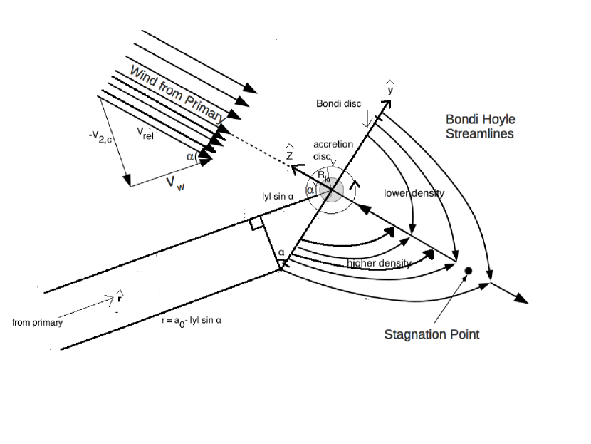
Figure 1: Schematic showing the flow structure of the binary wind capture process used in the “standard” approach to calculate the radius of disc formation. The figure is shown in the instantaneous inertial rest frame frame of the secondary. In the lab frame the secondary would be orbiting counterclockwise from this top view. The higher density of lines indicate a higher density of wind material because that part of the flow is closer to the primary. The purported radius of the accretion disk forming about the secondary is shown as $R_{k}$ as discussed and computed in section 2. As stated in the text, we assume $sin\alpha<<1$ but we have exaggerated the angle in the figure for clarity. The Bondi disc seen edge-on is indicated by the line segment between the two hash marks on the $\hat{\bf y}$ axis.

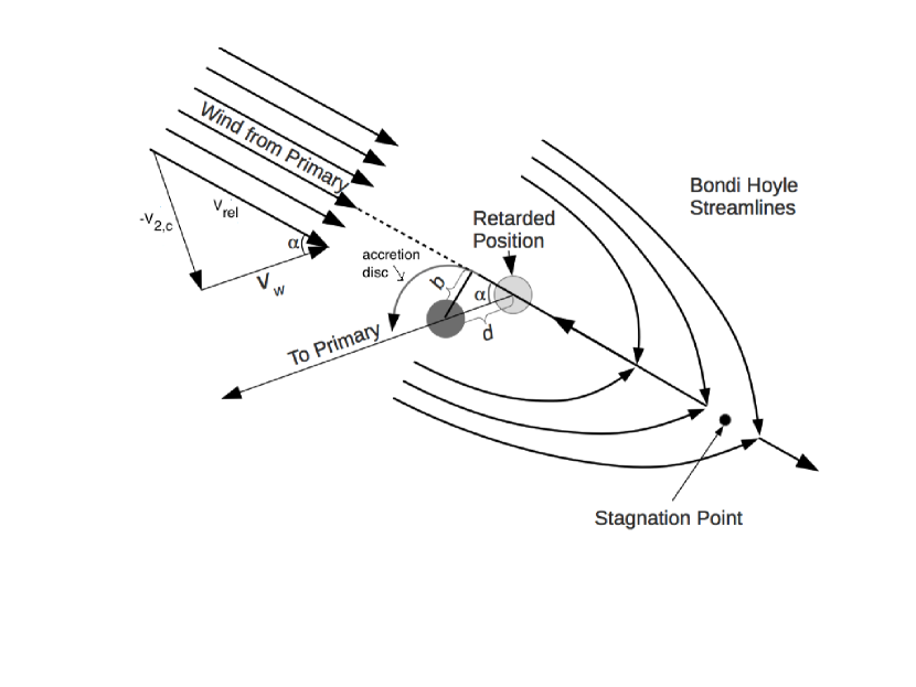
Figure 2: Same as Fig.1 except that here the density variation across the Bondi cylinder is ignored, and instead the acceleration of the secondary toward the primary relative to that of the wind is included. The two positions of the secondary that are shown at different times highlights that this figure is drawn in the inertial frame at the retarded time not the rotating frame. This leads to the accretion stream falling toward a retarded position of the secondary and the formation of an accretion disc with radius $b$ as discussed in the text.

To calculate the predicted disc scale analogue of (21) from the retardation effect, note that the time scale, $t_{c}$, associated with the wind capture process scales approximately with the time scale for material to flow from the stagnation point to the retarded position of the secondary. It takes approximately a free-fall time, $t_{ff}$, for material to fall toward the secondary, and the stagnation point is at least as large as the Bondi radius so a conservative estimate of $t_{c}$ can be made by assuming the material falls a displacement, $r_{b}$, giving

$$t_{c}\simeq t_{ff}={\pi\over 2}\frac{r_{b}^{3/2}}{(2GM_{2})^{1/2}}\sim\frac{r_{b}}{v_{rel}}.$$ (24)

During this time, the secondary is accelerated out of the instantaneous rest frame towards the primary relative to the wind with acceleration $A_{c}\sim\frac{v_{2,c}^{2}}{R_{2}}$. The distance, $d$, travelled by the secondary during the wind capture time scale $t_{c}$ is

$$d=\frac{1}{2}A_{c}t_{c}^{2},$$ (25)

and the distance perpendicular to the accretion column is the ASIP

$$b=d\sin{\alpha}=d\frac{v_{2,c}}{v_{rel}},$$ (26)

using the defintion of $\alpha$. Then using the expressions for $d$, $A_{c}$ and $t_{c}$ we obtain

$$b=\frac{v_{2,c}^{3}r_{b}^{2}(Q+1)}{2v_{rel}^{3}a_{o}Q}=\frac{r_{b}^{7/2}Q^{2}}{2^{5/2}a_{o}^{5/2}(Q+1)^{1/2}},$$ (27)

where in the first equality we have used Eq. (5) to convert from $R_{2}$ to $a_{o}$ and in the second equality we have used Eqn. (1) and (6).

We emphasize that $b$ measures the effective impact parameter of the accretion stream to the secondary, and the accretion stream moves approximately in free-fall from the stagnation point. Since the stagnation point is located at a position $\infty>r\mathrel{\hbox to0.0pt{\lower 4.0pt\hbox{\hskip 1.0pt$\sim$}\hss}\raise 1.0pt\hbox{$>$}}r_{b}$ from the point of closest approach, as long as $b<<r_{b}$, the flow at this position of closest approach would achieve a speed $v_{b}$ close to, but just below the escape speed. Specifically $v_{b}\approx\sqrt{2GM_{2}/b}$. This would correspond to a specific angular momentum of $j\approx\sqrt{2GM_{2}b}$ or a circular orbit or radius $\approx 2b$.

Having established that material at a displacement $b$ from the secondary meets the criterion of sufficient angular momentum, we can now ask which estimate, $b$ or $R_{K}$ determined in the previous section is larger. That will determine where the disc forms. The ratio of $b/R_{k}$ from (27) and (24) is

$${R_{k}\over b}=\frac{2^{1/2}r_{b}^{1/2}}{a_{o}^{1/2}(Q+1)^{1/2}}.$$ (28)

This ratio is important because in the present approximation that $r_{b}<<a_{o}$, we see that $b>R_{K}$. Because $b$ is the minimum scale for a disc to form around $M_{2}$ when the effect of wind acceleration is accounted even in the absence of a density gradient, such a disc will form at a larger radius than estimated by the method of the previous section. As an aside, note that the direction of angular momentum of the accretion disc is the same for both estimates (compare Figs. 1 and 2).

4 Conclusion

In a binary system where the primary is well within its Roche radius and accretion occurs onto the secondary via the well known BHL accretion of the primary’s wind, an accretion disc can still form around the secondary if the matter flowing onto the secondary has enough angular momentum to exceed the Keplerian speed of an orbit at its surface. We have considered the condition for initial disc formation for the case in which both the orbital separation well exceeds the Bondi accretion radius around the secondary and the orbital speed of the secondary is much less than the wind speed from the primary. We have shown that previous standard estimates for the size of the accretion disc, derived from combining the tilt between the binary radial separation vector and the axis of the Bondi accretion cylinder and the associated wind density variation across the Bondi cylinder, underestimate the disc radius.

The underestimate is a consequence of the incorrect assumption that the accretion stream follows a trajectory aimed toward the current position of the secondary. Correcting this assumption means taking into account the fact that the accretion stream is aimed at a retarded position of the secondary because the latter does not feel the accelerating force experienced by the wind. The secondary is drawn toward the primary by unfettered gravity during a Bondi accretion time. Equivalently one can consider the torque about the secondary applied by the wind on the accretion stream as it falls towards the secondary. The offset between the present and retarded positions of the secondary defines the ASIP in Eq. (23) which provides the larger accretion disc radius estimate as summarized by Eq. (28).

For the parameters of Huarte-Espinosa et al. (2013) $v_{2,c}/v_{w}\sim 0.5$ and $a_{o}/r_{b}~{}1.56$, so the regime is not quite the asymptotic regime that we have studied herein. Nevertheless, they were on the right track in emphasizing the potential importance of Eq. (23) as the minimum scale needed to numerically resolve the initial formation of an accretion disc from wind accretion by an orbiting secondary. (Once a substantial disc forms however, a higher resolution may be required to study the subsequent interaction between wind and disc.) Natural desired generalizations of the present work are indeed cases for which $r_{b}$ is not that much less than $a_{o}$ and/or $v_{w}<v_{2,c}$, and/or the density falls off faster than $1/r^{2}$. In such cases, the calculations of sections 2 and sections 3 should be revised to include higher order corrections. In such cases, the Bondi cylinder would be more strongly asymmetric in density so that the actual accretion disc radius would be a combination of the retardation effect and the density variation. In addition, if $r_{b}$ is comparable to $a_{o}$, the acceleration force of the wind would vary significantly over the scale of the accretion stream flow from the stagnation point to the secondary. Thus the relative acceleration of the secondary toward the primary compared to that of the wind would not be a constant, as we have assumed in this paper. but would spatially vary across the trajectory of the accretion stream. We leave these generalizations as future opportunities.

References

- (1) Abramowicz M.A. and Fragile. P.C., Living Rev. Relativity 16, (2013)
- (2) Abramowicz M.A. & Straub O., Accretion Discs, Scholarpedia, in press (2013); www.scholarpedia.org/article/Accretion_discs
- Balick & Frank (2002) Balick, B., & Frank, A. 2002, ARAA, 40, 439
- Blackman et al. (2001) Blackman, E. G., Frank, A., & Welch, C. 2001, ApJ, 546, 288 Blandford, R. D., & Payne, D. G. 1982, MNRAS, 199, 883
- (5) Bondi H., Hoyle F., 1944, MNRAS, 104, 273
- Bujarrabal et al. (2001) Bujarrabal, V., Castro-Carrizo, A., Alcolea, J., Sánchez Contreras, C., 2001, AAP, 377, 868
- De Marco (2009) De Marco, O. 2009, PASP, 121, 316
- (8) De Marco O., Soker N., 2011, PASP, 123, 402
- D’Souza et al. (2006) D’Souza, M. C. R., Motl, P. M., Tohline, J. E., & Frank, J. 2006, ApJ, 643, 381
- Edgar (2004) Edgar, R., 2004, New Ast. Rev., 48, 843
- Eggleton (1983) Eggleton, P. P. 1983, ApJ, 268, 368
- (12) Foglizzo T., Galletti P., Ruffert M., 2005, A&A, 435, 397
- (13) Frank J., King A., Raine D.J., 2002, Accretion Power in Astrophysics: Third Edition, Cambridge University Press, Cambridge.
- (14) Huarte-Espinosa M., Carroll-Nellenback J., Nordhaus J., Frank A., Blackman E. G., 2013, MNRAS, 433, 295
- (15) Jahanara B., Mitsumoto M., Oka K., Matsuda T., Hachisu I., Boffin H. M. J., 2005, A&A, 441, 589
- (16) Livio M., Soker N., de Kool M., Savonije G. J., 1986, MNRAS, 222, 235
- Mastrodemos & Morris (1998) Mastrodemos, N., & Morris, M., 1998, ApJ, 497, 303 Mohamed, S., & Podsiadlowski, P., 2007, Asymmetrical Planetary Nebulae IV Mohamed, S., & Podsiadlowski, P., 2011, Why Galaxies Care about AGB Stars II: Shining Examples and Common Inhabitants, 445, 355
- (18) Nagae T., Oka K., Matsuda T., Fujiwara H., Hachisu I., Boffin H. M. J., 2004, A&A, 419, 335
- (19) Nordhaus J., Blackman E. G., 2006, MNRAS, 370, 2004
- Perets & Kenyon (2012) Perets, H. B., & Kenyon, S. J., 2012, arXiv:1203.2918
- (21) Reyes-Ruiz M., López J. A., 1999, ApJ, 524, 952
- (22) Shapiro S. L., Lightman A. P., 1976, ApJ, 204, 555
- (23) Soker N., Livio M., 1984, MNRAS, 211, 927
- Soker & Rappaport (2000) Soker, N., & Rappaport, S., 2000, ApJ, 538, 241
- Soker & Rappaport (2001) Soker, N., & Rappaport, S. 2001, ApJ, 557, 256
- Theuns & Jorissen (1993) Theuns T., Jorissen A., 1993, MNRAS, 265, 946
- (27) Struck C., Cohanim B. E., Willson L. A., 2004, MNRAS, 347, 173
- (28) Theuns T., Jorissen A., 1993, MNRAS, 265, 946
- de Val-Borro et al. (2009) de Val-Borro, M., Karovska, M., & Sasselov, D., 2009, ApJ, 700, 1148
- (30) Wang Y.-M., 1981, A&A, 102, 36
- Witt et al. (2009) Witt, A. N., Vijh, U. P., Hobbs, L. M., et al., 2009, ApJ, 693, 1946