The gap distribution of slopes on the golden L

Abstract.

We give an explicit formula for the limiting gap distribution of slopes of saddle connections on the golden L, or any translation surface in its $\operatorname{SL}(2,\mathbb{R})$-orbit, in particular the double pentagon. This is the first explicit computation of the distribution of gaps for a flat surface that is not a torus cover.

1. Introduction

1.1. The golden L

The golden L is a translation surface obtained from an L-shaped polygon (with length ratios equal to the golden ratio $\varphi=\frac{1+\sqrt{5}}{2}$) by gluing opposite sides by horizontal and vertical translations (see Figure 1). It has genus two and a single cone-type singularity of angle $6\pi$ resulting from the identification of all vertices of the L-shaped polygon to a single point after the side gluings.

In this paper, we describe an explicit computation of the distribution of gaps between slopes of saddle connections on the golden L, where a saddle connection is a straight line trajectory starting and ending at the cone point of the golden L. This can be viewed as a geometric generalization of the gap distribution for Farey fractions [1].

Figure 1. Left: The golden L has sides glued pairwise by horizontal and vertical translations. All vertices, marked by dots, become a single point after side gluings. A saddle connection crossing a pair of identified sides is shown.

1.2. Translation structure

The side identifications of the golden L are by translations, which are holomorphic, so it inherits a Riemann surface structure, as well as a holomorphic one-form (from the form $dz$ in the plane, which is preserved by translations). This one-form $\omega$ on this Riemann surface has a single zero, of order two, at the cone-point of the golden L.

We identify the golden L to the one-form $\omega_{\mathrm{L}}$, the underlying Riemann surface being implied. The golden L and the closely related double pentagon have been popular objects of study and a testing ground for various properties of translation surfaces [7, 8].

1.3. Saddle connections and holonomy

Associated to each oriented saddle connection $\gamma$ is a holonomy vector, which we will call a saddle connection vector,

$$\mathbf{v}_{\gamma}=\int_{\gamma}\omega\in\mathbb{C},$$

which records how far and in what direction $\gamma$ travels. The set of saddle connection vectors,

$$\Lambda_{\omega}=\{\,\mathbf{v}_{\gamma}:\gamma\mbox{ an oriented saddle connection on the golden L}\,\}\subset\mathbb{C},$$

is a discrete subset of the plane with quadratic asymptotics [17]. Veech [22] showed that

$$|\Lambda_{\omega}\cap B(0,R)|\simeq c\mspace{1.0mu}R^{2},$$

where $a(R)\simeq b(R)$ indicates that the ratio of $a(R)$ and $b(R)$ goes to $1$ as $R\to\infty$, and where $c=3\mspace{1.0mu}\pi/10$ is the volume of $\mathbb{H}^{2}/\Gamma$, where $\Gamma=\triangle(2,5,\infty)$ is the Hecke $(2,5,\infty)$ triangle group, which is the Veech group of the golden L (see § 2.3).

1.4. Slopes and uniform distribution

The object of this paper is to study the distribution of the set of slopes of $\Lambda_{\omega}$. Since the set $\Lambda_{\omega}$ is symmetric about the coordinate axes as well as about the first and second diagonals, it is enough to study slopes of vectors in the first quadrant below the first diagonal,

$$\mathbb{S}=\left\{\operatorname{slope}(z)=\frac{\operatorname{Im}(z)}{\operatorname{Re}(z)}:z\in\Lambda_{\omega},\ 0\leq\operatorname{Im}(z)\leq\operatorname{Re}(z)\right\}\subset[0,1].$$

We view $\mathbb{S}$ as the union of the nested sets

$$\mathbb{S}_{R}=\left\{\operatorname{slope}(z)=\frac{\operatorname{Im}(z)}{\operatorname{Re}(z)}:z\in\Lambda_{\omega},\ 0\leq\operatorname{Im}(z)\leq\operatorname{Re}(z)\leq R\right\}.$$

In [22], Veech shows that not only the cardinality $N(R)=|\mathbb{S}_{R}|$ grows quadratically (as discussed above), but also the sets $\mathbb{S}_{R}$ become equidistributed in $[0,1]$ with respect to Lebesgue measure. That is, the uniform probability measure on the finite set $\mathbb{S}_{R}$ weak-$*$-converges to the Lebesgue probability measure on $[0,1]$:

$$\frac{1}{N(R)}\sum_{s\in\mathbb{S}_{R}}\delta_{s}\xrightarrow{\text{w}*}\lambda$$

(where $\delta_{s}$ denotes the Dirac mass at $s$). This result can be interpreted as saying that to the first order, the directions of saddle connections on the golden L appear randomly.

1.5. Gap distributions

A finer assessment of randomness arises from the gap distribution of the slopes. For $R\geq 1$ (so $\mathbb{S}_{R}$ is nonempty), index the elements of $\mathbb{S}_{R}$ in increasing order:

$$0=s_{R}^{(0)}<s_{R}^{(1)}<s_{R}^{(2)}<\ldots<s_{R}^{(N(R)-1)}=1$$

and consider the set of scaled differences or gaps (scaled by $R^{2}$ since $N(R)$ grows in $R^{2}$):

$$\mathbb{G}_{R}=\left\{R^{2}\left(s_{R}^{(i+1)}-s_{R}^{(i)}\right):0\leq i<N(R)-1\right\}.$$

We are interested in the limiting behavior of the probability measure supported on $\mathbb{G}_{R}$, in particular, for $0\leq a<b\leq+\infty$, the existence and evaluation of

(1.1) $$\lim_{R\rightarrow\infty}\frac{\left|\mathbb{G}_{R}\cap(a,b)\right|}{N(R)}.$$

If the slopes were ‘truly random’, obtained from sampling a sequence of independent identically distributed random variables following the uniform law on $[0,1]$, the associated gap distribution would be exponential, that is, the above limit would be $e^{-a}-e^{-b}$.

Our main result is the existence and computation of the gap distribution (1.1).

Theorem 1.1.

There is a limiting probability distribution function $f:[0,\infty)\rightarrow[0,\infty)$, with

$$\lim_{R\rightarrow\infty}\frac{\left|\mathbb{G}_{R}\cap(a,b)\right|}{N(R)}=\int_{a}^{b}f(x)dx.$$

This function $f$ is continuous, piecewise real-analytic, with seven points of non-differentiability, and the real-analytic pieces have explicit expressions involving usual functions.

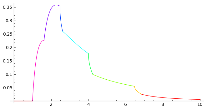
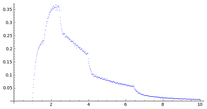
Figure 2. The limiting and empirical distributions for gaps of saddle connection slopes on the golden L. The empirical distribution is for saddle connection vectors of slope at most $1$ and horizontal component less than $10^{4}$.

Remark 1.

The formulas for the real-analytic pieces of the probability distribution function $f$ are given in Appendix A.

Remark 2.

The distribution has no support at $0$, in fact $f(x)=0$ for $0\leq x\leq 1$. The tail of the distribution is quadratic, that is, for $t\gg 0$,

$$\int_{t}^{\infty}f(x)dx\sim t^{-2},$$

where $\sim$ indicates that, for large enough $t$, the ratio is bounded between two positive constants. In particular, as is clear from Figure 2, the distribution is not exponential.

1.6. Typical surfaces

In [2], the first two authors considered gap distributions for typical translation surfaces, that is, surfaces in a set of full measure for the Masur-Veech measure (or, in fact, any ergodic $\operatorname{SL}(2,\mathbb{R})$-invariant measure) on a connected component of a stratum of the moduli space $\Omega_{g}$ of genus $g\geq 2$ translation surfaces.

It was shown that the limiting distribution exists, and is the same for almost every surface, and, as above, the tail is quadratic. In contrast to our setting, the distribution does have support at $0$ (for generic surfaces for the Masur-Veech measure). For lattice surfaces, of which the golden L is an example, the distribution does not have support at $0$, in fact, there are no small gaps. This is essentially equivalent to the no small triangles condition of Smillie-Weiss [20]. However, the only explicit computations in [2] were for branched covers of tori, and relied on previous work of Marklof-Strömbergsson [15] on the space of affine lattices. To the best of our knowledge, the current paper gives the first explicit computation of a gap distribution of saddle connections for a surface which is not a branched cover of a torus.

1.7. Strategy of proof

We follow the work of [3] where the first author and Y. Cheung, inspired by the work of Boca-Cobeli-Zaharescu [4] (also see [5] for a survey), gave an ergodic-theoretic proof of Hall’s Theorem [12] on the gap distribution of Farey fractions, using the horocycle flow on the modular surface. The key idea is to construct a Poincaré section for the horocycle flow on an appropriate moduli space, and to compute the distribution of the return time function with respect to an appropriate measure. This strategy can be used in many different situations, see [1] for a description of some of them.

2. Strata, $\operatorname{SL}(2,\mathbb{R})$-action, and Veech groups

In this section we relax the notations $\omega$, $\Lambda_{\omega}$ from their use in the previous section.

2.1. Strata of translation surfaces

A (compact, genus $g$) translation surface is given by a holomorphic one-form $\omega$ on a compact genus $g$ Riemann surface. Leaving the Riemann surface implicit, we simply refer to $\omega$ as the translation surface. More geometrically, a translation surface is given by a union of polygons $P_{1}\cup\dots\cup P_{n}\subset\mathbb{C}$, and gluings of parallel sides by translations, such that each side is glued to exactly one other, and the total angle at each vertex class is an integer multiple of $2\pi$. Since translations are holomorphic, and preserve $dz$, we obtain a complex structure and a holomorphic differential on the glued up surface. The zeros of the differential are at the identified vertices with total angle greater than $2\pi$. A zero of order $k$ is a point with total angle $2\pi(k+1)$. The sum of the angle excess is $2\pi(2g-2)$, where $g$ is the genus of the glued up surface. Equivalently the orders of the zeros sum up to $2g-2$.

Thus, the space of genus $g$ translation surfaces can be stratified by integer partitions of $2g-2$. If $\underline{k}=(k_{1},\ldots,k_{s})$ is a partition of $2g-2$, we denote by $\mathcal{H}(\underline{k})$ the moduli space of translation surfaces $\omega$ such that the multiplicities of the zeros are given by $k_{1},\dots,k_{s}$. The golden L is a genus $2$ surface with one zero of order $2$ (total angle $6\pi$), that is, $\omega\in\mathcal{H}(2)$.

2.2. Action of $\operatorname{SL}(2,\mathbb{R})$

The group $\operatorname{SL}(2,\mathbb{R})$ acts on each stratum $\mathcal{H}(\underline{k})$ via its action by linear maps on the plane: given a surface $\omega$ glued from polygons $P_{1}$, $\dots$, $P_{n}$ in the plane, define $g\cdot\omega$ as $gP_{1}\cup\dots\cup gP_{n}$, with the same side gluings for $g\cdot\omega$ as for $\omega$.

2.3. Veech groups and lattice surfaces

For a partition $\underline{k}$ of $2g-2$, with $g\geq 2$, and a typical surface $\omega\in\mathcal{H}(\underline{k})$, the stabilizer $\Gamma$ of $\omega$ in $\operatorname{SL}(2,\mathbb{R})$, known as the Veech group of $\omega$, is trivial. However, for a dense subset, the Veech group is a lattice in $\operatorname{SL}(2,\mathbb{R})$. These surfaces are known as lattice surfaces or Veech surfaces. While these lattices are never co-compact, Smillie [Smillie] showed that the $\operatorname{SL}(2,\mathbb{R})$-orbit of a translation surface $\omega$ is a closed subset of $\mathcal{H}(\underline{k})$ if and only if $\omega$ is a lattice surface, and in this setting it can be identified with the quotient $\operatorname{SL}(2,\mathbb{R})/\Gamma$. Thus, a general principle is the following:

Principle. If a problem about the geometry of a translation surface can be framed in terms of its $\operatorname{SL}(2,\mathbb{R})$ orbit, and $\omega$ is a lattice surface, then the problem can be reduced to studying the dynamics of the $\operatorname{SL}(2,\mathbb{R})$ action on the homogeneous space $\operatorname{SL}(2,\mathbb{R})/\Gamma$.

2.4. Veech group orbits and saddle connections

Recall that a saddle connection $\gamma$ on a translation surface $\omega$ is a geodesic in the flat metric determined by $\omega$ on the underlying Riemann surface, with both endpoints at zeros of $\omega$ and no zero of $\omega$ in its interior. The holonomy vector of $\gamma$ is given by

$$\mathbf{v}_{\gamma}=\int_{\gamma}\omega\in\mathbb{C}.$$

The set of holonomy vectors

$$\Lambda_{\omega}=\{\mathbf{v}_{\gamma}:\gamma\mbox{ is a saddle connection on }\omega\}\subset\mathbb{C}$$

is a discrete subset of the plane, which varies equivariantly under the $\operatorname{SL}(2,\mathbb{R})$-action, that is $\Lambda_{g\omega}=g\Lambda_{\omega}.$ When $\omega$ is a lattice surface, the set $\Lambda_{\omega}$ is a finite union of orbits of the Veech group $\Gamma$ acting linearly on $\mathbb{R}^{2}\backslash\{0\}$ (see, for example [13]). That is, there are vectors $\mathbf{v}_{1},\ldots,\mathbf{v}_{k}\in\mathbb{R}^{2}\backslash\{0\}$ such that

$$\Lambda_{\omega}=\bigcup_{i=1}^{k}\Gamma\mathbf{v}_{i}.$$

In the setting of the golden L, we have two vectors $\mathbf{v}_{1}=\frac{\sqrt{5}-1}{2}$ and $\mathbf{v}_{2}=1$, viewed as complex numbers. Since we are interested in the slopes of vectors, and $\mathbf{v}_{1}$ and $\mathbf{v}_{2}$ are collinear, we work with the orbit $\Gamma\mathbf{v}_{2}$, where $\Gamma=\Gamma(\omega)=\triangle(2,5,\infty)$. We fix the notation $\Gamma=\triangle(2,5,\infty)$ in the rest of this paper, and let $\Lambda=\Gamma\mathbf{v}_{2}\subset\Lambda_{\omega}$.

3. Horocycle flows and first return maps

In the rest of the paper, $\omega$ denotes the golden L, $\Gamma$ denotes its Veech group, the $(2,5,\infty)$ triangle group, and $\Lambda$ denotes the subset $\Gamma\mathbf{v}_{2}$ of $\Lambda_{\omega}$ described at the end of section 2.

3.1. Horocycle flow and slope gaps

The key tool in the proof of Theorem 1.1 is the construction of a first return map for the horocycle flow on the $\operatorname{SL}(2,\mathbb{R})$-orbit of $\omega$, which, as discussed above, can be identified with the homogeneous space $\operatorname{SL}(2,\mathbb{R})/\Gamma$. For our purposes, the horocycle flow is given by the (left) action of the subgroup:

$$\left\{h_{s}=\begin{bmatrix}1&0\\ -s&1\end{bmatrix}:s\in\mathbb{R}\right\}.$$

We also define, for $a,b\in\mathbb{R}$ with $a\neq 0$, the matrix

$$g_{a,b}=\begin{bmatrix}a&b\\ 0&a^{-1}\end{bmatrix}.$$

Slope gaps.

Note that if $z\in\mathbb{C}$, and $\operatorname{slope}(z)=\operatorname{Im}(z)/\operatorname{Re}(z)$ is the slope, we have

$$\operatorname{slope}(h_{s}z)=\operatorname{slope}(z)-s,$$

since $\operatorname{Re}(h_{s}z)=\operatorname{Re}(z)$, $\operatorname{Im}(h_{s}z)=\operatorname{Im}(z)-s\operatorname{Re}(z)$. Thus, the action of $h_{s}$ preserves differences in slopes. Thus to understand the slope gaps of $\Lambda$ (or more generally of $g\Lambda$ for $g\in\operatorname{SL}(2,\mathbb{R})$), it is useful to consider the orbit of $\Lambda$ under $h_{s}$.

3.2. A Poincaré section

Following [1, 3], we build a cross-section to the flow $h_{s}$ on the space $X=\operatorname{SL}(2,\mathbb{R})/\Gamma$. Let $\Omega_{X}\subset X$ be given by

(3.1) $$\Omega_{X}=\{g\Gamma:g\Lambda\cap(0,1]\neq\emptyset\},$$

where we view $(0,1]$ as the horizontal segment $\{0<x\leq 1\}\subset\mathbb{C}$. That is, $\Omega_{X}$ consists of surfaces in the $\operatorname{SL}(2,\mathbb{R})$ orbit of $\omega$ which contain a short (length $\leq 1$) horizontal vector.

Theorem 3.1.

The subset $\Omega_{X}\subset X$ is a Poincaré section to the horocycle flow $h_{s}$ on $X$. Moreover, the map $(a,b)\mapsto g_{a,b}\Gamma$ establishes a bijection

$$\Omega=\{(a,b)\in\mathbb{R}^{2}:0<a\leq 1,1-a\varphi<b\leq 1\}\longrightarrow\Omega_{X}.$$

In these coordinates, the return map $T:\Omega\rightarrow\Omega$ is a measure-preserving bijection, piecewise linear with countably many pieces. The return time function $R:\Omega\rightarrow\mathbb{R}^{+}$ defined by

$$R(a,b)=\min\{s>0:h_{s}g_{a,b}\Gamma\in\Omega_{X}\}$$

is a piecewise rational function with three pieces, and is uniformly bounded below by $1$. We call the map $T$ the golden-L BCZ map.

3.3. Connection to slope gaps

The connection between Theorem 3.1 and slope gap distributions can be seen as follows. For $g\in\operatorname{SL}(2,\mathbb{R})$, consider the set of positive slopes $\mathbb{S}^{g}_{1}=\{s_{1}<s_{2}<\ldots<s_{N}<\ldots\}$ of elements of $g\Lambda\cap U_{1}$, where $U_{1}$ is the vertical strip

$$U_{1}=(0,1]\times(0,+\infty)=\{z\in\mathbb{C}:\operatorname{Im}(z)>0,\operatorname{Re}(z)\in(0,1]\}.$$

These slopes are the positive times $s$ when the orbit $\{h_{s}g\Gamma\}_{s>0}$ intersects $\Omega_{X}$. That is,

$$h_{s_{i}}g\Gamma\in\Omega_{X},\hskip 5.69054pti=1,2,\ldots$$

Let $(a,b)\in\Omega$ be such that $h_{s_{1}}g\Gamma=g_{a,b}\Gamma$. Then we have, for $i\in\mathbb{N}$, $R(T^{i}(a,b))=s_{i+2}-s_{i+1}$. That is, the set of gaps $\mathbb{G}^{N}_{g}=\{s_{i+1}-s_{i}:i=1,2,3,\ldots N\}$ is given by the roof function $R$ evaluated along the orbit of the return map $T$ up till time $N-1$. For $t>0$, the proportion of gaps of size at most $t$ can be expressed as a Birkhoff sum of the indicator function $\chi_{t}$ of the set $R^{-1}([t,\infty))\subset\Omega$, via

$$\frac{1}{N}|\mathbb{G}^{N}_{g}\cap[t,\infty)|=\frac{1}{N}\sum_{i=0}^{N-1}\chi_{t}(T^{i}(a,b)).$$

Thus, the dynamics and ergodic theory of the return map (and in particular the distribution of the roof function along orbits) are crucial to understanding the gap distributions of slopes.

3.4. Proof of Theorem 3.1

Let $a_{t}=g_{e^{t/2},0}$ and $u_{s}=g_{1,s}$. The action of $a_{t}$ is known as the geodesic flow and the action of $u_{s}$ is the (opposite) horocycle flow. For $x=g\Gamma\in X$, let $\ell(x)=\min\{|g\mathbf{v}|:\mathbf{v}\in\Lambda\}$ denote the length of the shortest nonzero vector in $g\Lambda$. For any compact subset $K\subset X$, there is an $\epsilon>0$ such that for any $x\in K$, $\ell(x)>\epsilon$. Given $x=g\Gamma\in X$, the following are equivalent (see, e.g., [13]):

• $u_{s}$-periodicity: there exists $s_{0}\neq 0$ so that $u_{s_{0}}x=x$.

• $a_{-t}$-divergence: as $t\to+\infty$, $a_{-t}x\to\infty$ in $X$. In particular, $\ell(a_{-t}x)\to 0$.

• $x$ has a horizontal saddle connection, that is, there exists $\mathbf{v}\in g\Lambda\cap\mathbb{R}$.

• upper triangular form: we can write $x=g_{a,b}\Gamma$, where $a=\min\{|\mathbf{v}|:\mathbf{v}\in g\Lambda\cap\mathbb{R}\}$ is the length of the shortest horizontal vector in $g\Lambda$.

Similarly, $h_{s}$-periodicity is equivalent to $a_{t}$-divergence and having a vertical saddle connection.

Recall that $\Omega_{X}$ is the set of surfaces in the $\operatorname{SL}(2,\mathbb{R})$-orbit of the golden L with a length $\leq 1$ horizontal long saddle connection vector. By the above, these can be expressed as $g_{a,b^{\prime}}\Gamma\in X$, with $0<a\leq 1$, and $b^{\prime}\in\mathbb{R}$. Since the parabolic element $u_{-\varphi}$ is in $\Gamma$, we can apply it $k$ times on the right to $g_{a,b^{\prime}}$ to obtain $g_{a,b^{\prime}-k\varphi a}$, where $b=b^{\prime}-k\varphi a\in(1-\varphi a,1]$. This condition determines $b$ uniquely (and given any starting $b^{\prime}$, it determines $k$). Conversely, any surface of the form $g_{a,b}\omega$ with $(a,b)\in\Omega$ has the saddle connection vector $a\in\mathbb{C}$, and thus clearly has a horizontal vector of length at most $1$. Thus, we have shown that $\Omega_{X}$ and $\Omega$ are in bijection.

Figure 3. Left: Vectors $w_{j}$ in $\Lambda$ (the orbit $\Gamma\mathbf{v}_{2}$) of slopes $j=0$, ${\overline{\varphi}}$, $1$, $\varphi$, $\infty$.
Right: The partition of $\Omega$ into $\Omega_{1}$, $\Omega_{\varphi}$, $\Omega_{\infty}$.

To calculate the return time and the return map, we need to understand the vector in $g_{a,b}\Lambda$ of smallest positive slope in the vertical strip $U_{1}$. In Figure 3, we show a selection of vectors in $\Lambda$. Particularly relevant to our discussion are the vectors $w_{1}=(\varphi,\varphi)$, $w_{\varphi}=(1,\varphi)$, $w_{\infty}=(0,1)$.

Consider the partition of $\Omega$ into the three subdomains $\Omega_{1}$, $\Omega_{\varphi}$, $\Omega_{\infty}$ defined by:

$$\Omega_{1} =\bigl{\{}\,(a,b)\in\Omega:\hskip 5.69054pt{\overline{\varphi}}\leq a\leq 1,\hskip 5.69054pt1-a\varphi<b\leq{\overline{\varphi}}-a\,\bigr{\}}$$

$$\Omega_{\varphi} =\bigl{\{}\,(a,b)\in\Omega:\hskip 5.69054pt{\overline{\varphi}}^{2}\leq a\leq 1,\hskip 5.69054pt{\overline{\varphi}}-a<b\leq{\overline{\varphi}}-a{\overline{\varphi}}\,\bigr{\}}$$

$$\Omega_{\infty} =\bigl{\{}\,(a,b)\in\Omega:\hskip 5.69054pt0<a\leq 1,\hskip 5.69054pt{\overline{\varphi}}-a{\overline{\varphi}}<b\leq 1\,\bigr{\}}$$

These subdomains are illustrated in Figure 3.

A direct calculation, left as an exercise to the reader, shows that for each $j$ in $\{1,\varphi,\infty\}$, for any $(a,b)$ in $\Omega_{j}$, the vector $g_{a,b}w_{j}$ is the one with smallest slope in $g_{a,b}\Lambda\cap U_{1}$.

In each zone, the return time is given by the slope of the corresponding vectors. Thus,

•–if $(a,b)\in\Omega_{1}$,  $g_{a,b}w_{1}=\varphi((a+b)+a^{-1}i)$,  and  $R(a,b)=\frac{a^{-1}}{a+b}\frac{1}{a(a+b)}$;

•–if $(a,b)\in\Omega_{\varphi}$,  $g_{a,b}w_{\varphi}=(a+b\varphi)+a^{-1}\varphi i$,  and   $R(a,b)=\frac{a^{-1}\varphi}{a+b\varphi}=\frac{1}{a(a{\overline{\varphi}}+b)}$;

•–if $(a,b)\in\Omega_{1}$,  $g_{a,b}w_{\infty}=b+a^{-1}i$,  and   $R(a,b)=\frac{a^{-1}}{b}=\frac{1}{ab}$.

To compute the return map, Note that $h_{s}g_{a,b}=\begin{bmatrix}a&b\\ -sa&-sb+a^{-1}\end{bmatrix}$ is then respectively $\begin{bmatrix}a&b\\ \frac{-1}{a+b}&\frac{1}{a+b}\end{bmatrix}$, $\begin{bmatrix}a&b\\ \frac{-1}{a{\overline{\varphi}}+b}&\frac{{\overline{\varphi}}}{a{\overline{\varphi}}+b}\end{bmatrix}$, $\begin{bmatrix}a&b\\ \frac{-1}{b}&0\end{bmatrix}$.

Computing the canonical representative $g_{T(a,b)}$ in the class $h_{s}g_{a,b}\Gamma$ yields:

•–in $\Omega_{1}$: $\displaystyle\begin{bmatrix}a&b\\ \frac{-1}{a+b}&\frac{1}{a+b}\end{bmatrix}\begin{bmatrix}\varphi&1\\ \varphi&\varphi\end{bmatrix}u_{\varphi}^{k_{1}}=\begin{bmatrix}(a+b)\varphi&a+b\varphi+k_{1}\varphi^{2}(a+b)\\ 0&\frac{{\overline{\varphi}}}{a+b}\end{bmatrix}$, $k_{1}=-\left\lfloor\frac{a+b\varphi-1}{\varphi^{2}(a+b)}\right\rfloor$,

•–in $\Omega_{\varphi}$: $\displaystyle\begin{bmatrix}a&b\\ \frac{-1}{a{\overline{\varphi}}+b}&\frac{{\overline{\varphi}}}{a{\overline{\varphi}}+b}\end{bmatrix}\begin{bmatrix}1&0\\ \varphi&1\end{bmatrix}u_{\varphi}^{k_{p}hi}=\begin{bmatrix}a+b\varphi&b+k_{\varphi}\varphi(a+b\varphi)\\ 0&\frac{{\overline{\varphi}}}{a{\overline{\varphi}}+b}\end{bmatrix}$, $k_{\varphi}=-\left\lfloor\frac{b-1}{\varphi(a+b\varphi)}\right\rfloor$,

•–in $\Omega_{\infty}$: $\displaystyle\begin{bmatrix}a&b\\ \frac{-1}{b}&0\end{bmatrix}\begin{bmatrix}0&-1\\ 1&0\end{bmatrix}u_{\varphi}^{k_{\infty}}=\begin{bmatrix}b&-a+k_{\infty}\varphi b\\ 0&\frac{1}{b}\end{bmatrix}$, $k_{\infty}=-\left\lfloor\frac{-a-1}{\varphi b}\right\rfloor$.

Thus, we have the following formulas for $T(a,b)$:

•–in $\Omega_{1}$: $T(a,b)=\left((a+b)\varphi,a+b\varphi+k_{1}\varphi^{2}(a+b)\right)$, $k_{1}=-\left\lfloor\frac{a+b\varphi-1}{\varphi^{2}(a+b)}\right\rfloor$,

•–in $\Omega_{\varphi}$: $T(a,b)=\left(a+b\varphi,b+k_{\varphi}\varphi(a+b\varphi)\right)$, $k_{\varphi}=-\left\lfloor\frac{b-1}{\varphi(a+b\varphi)}\right\rfloor$,

•–in $\Omega_{\infty}$: $T(a,b)=(b,-a+k_{\infty}\varphi b)$, $k_{\infty}=-\left\lfloor\frac{-a-1}{\varphi b}\right\rfloor$.

This completes the proof of Theorem 3.1.∎

4. Ergodicity and equidistribution

4.1. Ergodic theory for $T$

The construction of the map $T$ as a first return map for horocycle flow on $X=\operatorname{SL}(2,\mathbb{R})/\Gamma$ allows us to classify the ergodic invariant measures for $T$ and that long periodic orbits of $T$ equidistribute, as consequences of the corresponding results for $h_{s}$ acting on $\operatorname{SL}(2,\mathbb{R})/\Gamma$, due to Dani-Smillie [6].

Theorem 4.1.

The Lebesgue probability measure $m$ given by $dm=\frac{2}{\varphi}dadb$ is the unique ergodic invariant probability measure for $T$ not supported on a periodic orbit. In particular it is the unique ergodic absolutely continuous invariant measure (acim). For every $(a,b)$ not periodic under $T$ and any function $f\in L^{1}(\Omega,dm)$, we have that

$$\lim_{N\rightarrow\infty}\frac{1}{N}\sum_{i=0}^{N-1}f(T^{i}(a,b))=\int_{\Omega}fdm$$

Moreover, if $\{(a_{r},b_{r})\}_{r=1}^{\infty}$ is a sequence of periodic points with periods $N(r)\rightarrow\infty$ as $r\rightarrow\infty$, we have, for any bounded function $f$ on $\Omega$,

$$\lim_{r\rightarrow\infty}\frac{1}{N(r)}\sum_{i=0}^{N(r)-1}f(T^{i}(a_{r},b_{r}))=\int_{\Omega}fdm.$$

Proof.

By standard theory of first return maps, if $(a,b)$ is not periodic with respect to $T$, then $g_{a,b}\Gamma$ is not $h_{s}$-periodic. By the results of Dani-Smillie [6], non-periodic orbits of $h_{s}$ equidistribute (i.e., are Birkohff regular) with respect to Haar measure $\mu$ on $\operatorname{SL}(2,\mathbb{R})/\Gamma$, which can be described as (a multiple of) $dadbds$ when we realize $\operatorname{SL}(2,\mathbb{R})/\Gamma$ as a suspension space over $\Omega$ (see also Appendix B for detailed volume computations). Thus, the corresponding non-periodic orbit of $T$ on $\Omega$ must equidistribute with respect to Lebesgue measure on $\Omega$. Similarly, by results of Sarnak [19], long periodic horocycles on $\operatorname{SL}(2,\mathbb{R})/\Gamma$ equidistribute, and thus, long periodic orbits of $T$ on $\Omega$ must equidistribute. Since the roof function $R$ is bounded below by $1$, the length of the discrete period $N(r)\rightarrow\infty$ implies that the length of the continuous period of $g_{a_{r},b_{r}}\Gamma$ must also go to infinity (in fact, it is at least $N(r)$). ∎

4.2. Proof of main theorems

Before proving Theorem 1.1, we state and prove a more general result:

Theorem 4.2.

Let $x=g\Gamma\in X$ be such that $x$ is not $h_{s}$-periodic. Let

$$\mathbb{S}_{g}=\{0\leq s_{1}<s_{2}<\ldots<s_{N}<\ldots\}$$

be the set of slopes of elements of $g\Lambda$ in the vertical strip $U_{1}$. Let

$$\mathbb{G}^{N}_{x}=\{s_{i+1}-s_{i}:i=1,2,\ldots,N\}$$

denote the associated gap set. Then for any $t\geq 0$,

$$\lim_{N\rightarrow\infty}\frac{1}{N}\Bigl{\lvert}\mathbb{G}^{N}_{x}\cap[t,\infty)\Bigr{\rvert}=m(\bigl{\{}\,(a,b)\in\Omega:R(a,b)\geq t\,\bigr{\}}).$$

If $x=g\Gamma$ is $h_{s}$-periodic, define $x_{r}=a_{-r}g\Gamma=a_{-r}x$. Then there is a $P(r)$ so that for any $N\geq P(r)$, $\mathbb{G}^{N}_{x_{r}}=\mathbb{G}^{P(r)}_{x_{r}}.$ We then have

$$\lim_{r\rightarrow\infty}\frac{1}{P(r)}\Bigl{\lvert}\mathbb{G}^{P(r)}_{x_{r}}\cap[t,\infty)\Bigr{\rvert}=m(\bigl{\{}\,(a,b)\in\Omega:R(a,b)\geq t\,\bigr{\}}).$$

Proof.

As observed in §3.3, the proportion $\frac{1}{N}|\mathbb{G}^{N}_{x}\cap[t,\infty)|$ of the first $N$ slope gaps of size at most $t$ in the strip $U_{1}$ is a Birkhoff sum of the indicator function of the super-level set $\{(a,b)\in\Omega:R(a,b)\geq t\}$. The first statement then follows from the first statement of Theorem 4.1. For the second statement, note that if $x$ is periodic under $h_{s}$ with period $s_{0}$, $a_{-r}x$ is periodic with period $e^{r}s_{0}$, by the conjugation relation $a_{r}h_{s}a_{-r}=h_{se^{-r}}$. $P(r)$ is the corresponding period for the map $T$. The second statement of the theorem then follows from the second statement of Theorem 4.1. ∎

4.3. Proof of Theorem 1.1

Lemma 4.3.

Let $x$ be the golden L and $x_{R}=a_{-2\log R}x$. We have

$$\frac{\left|\mathbb{G}_{R}(\Lambda)\cap[t,\infty)\right|}{N(R)}=\frac{1}{N(R)}|\mathbb{G}^{N(R)}_{x_{R}}\cap[t,\infty)|.$$

Proof.

The golden L is $h_{s}$-periodic, with period $\varphi$, since the matrix $\begin{bmatrix}1&0\\ -\varphi&1\end{bmatrix}\in\Gamma$. We are interested in the slopes of saddle connections with horizontal component at most $R$, and slope at most $1$. The map $T$ does not see any of the saddle connections slopes for vectors of length more than $1$. However, renormalizing by the matrix $a_{-2\log R}=\begin{bmatrix}1/R&0\\ 0&R\end{bmatrix}$, we can consider the point $x_{R}=a_{-2\log R}\Gamma\in X$. Note that this matrix scales slopes and thus differences of slopes by $R^{2}$. Each $\gamma\in\mathbb{S}_{R}$ corresponds with a saddle connection $a_{-2\log R}\gamma$ on $x_{R}$ which is in $\Omega$. The point $x_{R}$ has period $N(R)$ under $T$. ∎

Proof of Theorem 1.1.

By Theorem 4.2 we have

$$\frac{1}{N(R)}\,\Bigl{\lvert}\mathbb{G}^{N(R)}_{x_{R}}\cap(t,\infty)\Bigr{\rvert}\to m(\bigl{\{}(a,b)\in\Omega:R(a,b)\geq t\bigr{\}}).$$

So by the previous lemma

$$\frac{1}{N(R)}\mspace{1.0mu}\bigl{\lvert}\mathbb{G}_{R}(\Lambda)\cap[t,\infty)\bigr{\rvert}\to m(\bigl{\{}(a,b)\in\Omega:R(a,b)\geq t\bigr{\}}).$$

∎

4.4. Spacings and statistics

The equidistribution of periodic points also yields significant further information on higher-order spacings and statistics for the gap distribution. We record one representative result on $h$-spacings, and refer the reader to [3, §1.5] for further results of this type in the setting of the torus, whose proofs can be easily modified to this setting.

Theorem 4.4.

Let $h$ be a positive integer, and let $t_{1},t_{2},\ldots,t_{h}>0$. Then the $h$-spacing distribution

$$\frac{1}{N(R)}\mspace{1.0mu}\Bigl{\lvert}\Bigr{\{}\,1\leq i\leq N(R):R^{2}(s^{(i+k)}_{R}-s^{(i+k-1)}_{R})>t_{k},\hskip 5.69054pt1\leq k\leq h\,\Bigr{\}}\Bigr{\rvert}$$

converges, as $R\to\infty$, to

$$m(\bigl{\{}(a,b)\in\Omega:R(T^{j}(a,b))\geq t_{j},0\leq j<h\bigr{\}})$$

Proof.

Apply the periodic case of Theorem 4.2 to the indicator function of the set

$$\bigl{\{}(a,b)\in\Omega:R(T^{j}(a,b))\geq t_{j},0\leq j<h\bigr{\}}.$$

∎

5. Further questions

Our method to explicitly compute the gap distribution in this setting leads us to several natural questions.

5.1. Real analyticity

Question.

Is the gap distribution for a generic (with respect to Masur-Veech measure on a stratum $\mathcal{H}(\underline{k})$ surface real analytic?

This distribution was shown to exist in [2], and in [1], a possible method of computing it by constructing a first return map for the action of $h_{s}$ on the stratum $\mathcal{H}(\underline{k})$ was suggested. However, explicitly computing this return map (or indeed the return time, which is the only requirement for the gap distribution) seems difficult. Perhaps a property like real analyticity is within reach. Our computation here shows that the distribution for the golden L is piecewise real-analytic. For the torus, this was computed by [12], and was real-analytic on 3 pieces. This leads to the natural

Question.

Is the gap distribution for all lattice surfaces piecewise real analytic?

We conjecture the answer is yes, and that the number of pieces are some measure of the ‘complexity’ of the Veech surface.

5.2. Support at 0

In [2] it was shown that lattice surfaces have no small (normalized) gaps, and that in contrast, that the gap distribution for generic surfaces has support at $0$. This leaves open the question:

Question.

Is there a translation surface whose gap distribution has no support at $0$ but does have small gaps. That is, for all $\epsilon>0$, for all $R\gg 0$, there exists a gap of slopes of saddle connections of length at most $R$ less than $\epsilon/R^{2}$, but there is an $\epsilon_{0}>0$ so that the proportion of gaps of size at most $\epsilon_{0}/R^{2}$ goes to $0$ as $R\rightarrow\infty$.

A possible set of candidates for such a surface might be completely periodic surfaces which are not lattice surfaces.

A. Explicit formulas for the probability distribution function

Notation.

•–We use a bar to denote the inverse, so $\overline{\alpha}$ and ${\overline{\varphi}}$ denote $\alpha^{-1}$ and $\varphi^{-1}$.
•–We denote by $\operatorname{ath}$ the inverse hyperbolic tangent function: $\operatorname{ath}(x)=(1/2)\ln((1+x)/(1-x))$.
•–We denote by $r$ the function $x\mapsto r(x)=\sqrt{1-4\mspace{1.0mu}x}$.

The cumulative distribution function for the gaps in slopes is the function $F$ which to $\alpha$ associates the probability $F(\alpha)$ that a gap is less than $\alpha$. The probability distribution function $f$ is the derivative of $F$.

We can see $F$ as the sum of three partial cdfs $F_{s}$ for the zones $\Omega_{s}$, for each $s\in\{1,\varphi,\infty\}$, where $F_{s}(\alpha)=\operatorname{area}\bigl{(}\Omega_{s}\cap(R_{s}(x,y)<\alpha)\bigr{)}$, giving the formulas $F_{\infty}(\alpha)=\operatorname{area}\bigl{(}\Omega_{\infty}\cap(xy>\overline{\alpha})\bigr{)}$, $F_{\varphi}(\alpha)=\operatorname{area}\bigl{(}\Omega_{\varphi}\cap(x({\overline{\varphi}}x+y)>\overline{\alpha})\bigr{)}$, and $F_{1}(\alpha)=\operatorname{area}\bigl{(}\Omega_{1}\cap(x(x+y)>\overline{\alpha})\bigr{)}$.

The different configurations, as $\alpha$ varies, of the intersection of the hyperbolas $R_{s}(x,y)=\alpha$ with the domains $\Omega_{s}$ determine different evaluations of these formulas; which by differentiating give the partial pdfs:

•–Respectively for:

$0<\alpha<1$,  $1<\alpha<4\varphi$,  $4\varphi<\alpha<\varphi^{4}$,  $\varphi^{4}<\alpha$,

•–$F_{\infty}(\alpha)$ equals:	$0$,  $1-\overline{\alpha}(1+\ln\alpha)$,  $1-\overline{\alpha}(1+\ln\alpha-4\operatorname{ath}r(\varphi\overline{\alpha}))-{\overline{\varphi}}\mspace{1.0mu}r(\varphi\overline{\alpha})$,
	$3{\overline{\varphi}}/2-\overline{\alpha}(1+2\ln({\overline{\varphi}}\alpha/2)+2\ln(1-r(\varphi\overline{\alpha})))+({\overline{\varphi}}/2)r(\varphi\overline{\alpha})$;

•–$f_{\infty}(\alpha)$ equals:

$0$,  $\overline{\alpha}^{2}\ln\alpha$,  $\overline{\alpha}^{2}(\ln\alpha-4\operatorname{ath}r(\varphi\overline{\alpha}))$,  $\overline{\alpha}^{2}(2\ln({\overline{\varphi}}\alpha/2)+2\ln(1-r(\varphi\overline{\alpha})))$.

•–Respectively for:

$0<\alpha<\varphi$,  $\varphi<\alpha<4$,  $4<\alpha<\varphi^{3}$,  $\varphi^{3}<\alpha$,

•–$F_{\varphi}(\alpha)$ equals:

$0$,  ${\overline{\varphi}}-\overline{\alpha}(1+\ln{{\overline{\varphi}}\alpha})$,  ${\overline{\varphi}}-\overline{\alpha}(1+\ln{{\overline{\varphi}}\alpha}-4\operatorname{ath}r(\overline{\alpha}))-r(\overline{\alpha})$,  ${\overline{\varphi}}^{4}$;

•–$f_{\varphi}(\alpha)$ equals:

$0$,  $\overline{\alpha}^{2}\ln{{\overline{\varphi}}\alpha}$,  $\overline{\alpha}^{2}(\ln{{\overline{\varphi}}\alpha}-4\operatorname{ath}r(\overline{\alpha}))$,  $0$.

•–Respectively for:

$0<\alpha<\varphi$,  $\varphi<\alpha<4{\overline{\varphi}}$,  $4{\overline{\varphi}}<\alpha<\varphi^{2}$,  $\varphi^{3}<\alpha$,

•–$F_{1}(\alpha)$ equals:

$0$,  ${\overline{\varphi}}-\overline{\alpha}(1+\ln{{\overline{\varphi}}\alpha})$,  ${\overline{\varphi}}-\overline{\alpha}(1+\ln{{\overline{\varphi}}\alpha}-2\operatorname{ath}r({\overline{\varphi}}\overline{\alpha}))-(\varphi/2)\mspace{1.0mu}r({\overline{\varphi}}\overline{\alpha})$,  ${\overline{\varphi}}^{5}/2$;

•–$f_{1}(\alpha)$ equals:

$0$,  $\overline{\alpha}^{2}\ln{{\overline{\varphi}}\alpha}$,  $\overline{\alpha}^{2}(\ln{{\overline{\varphi}}\alpha}-2\operatorname{ath}r({\overline{\varphi}}\overline{\alpha}))$,  $0$.

B. Volume computations

Define a measurable partition of $X=\operatorname{SL}(2,\mathbb{R})/\Gamma$ into $X_{1}$, $X_{\varphi}$, $X_{\infty}$ where each $X_{j}$ is the part of $X$ spanned by $\Omega_{j}$ under the flow $(h_{s})$, until its first return to $\Omega$. The complement of the union of the $X_{j}$’s is the union of periodic orbits for the flow $(h_{s})$, which has measure zero. The partial volumes $V_{j}=\operatorname{vol}(X_{j})=\int_{\Omega_{j}}R$ are obtained by integrating the return time function $R(a,b)$ over the domains $\Omega_{j}$.

•–Integrating $R$ over $\Omega_{1}$,

$$V_{1} =\int_{a={\overline{\varphi}}}^{1}\int_{b=1-a\varphi}^{{\overline{\varphi}}-a}\dfrac{1}{a(a+b)}\;da\,db=\int_{{\overline{\varphi}}}^{1}\Bigl{[}\ln(a+b)\Bigr{]}_{1-a\varphi}^{{\overline{\varphi}}-a}\;\dfrac{da}{a}=\int_{{\overline{\varphi}}}^{1}\Bigl{(}\ln({\overline{\varphi}})-\ln(1-a{\overline{\varphi}})\Bigr{)}\;\dfrac{da}{a}$$

$$=-(\ln{\overline{\varphi}})^{2}-\int_{{\overline{\varphi}}^{2}}^{{\overline{\varphi}}}\ln(1-t)\;\dfrac{dt}{t}=-(\ln\varphi)^{2}+\operatorname{Li}_{2}({\overline{\varphi}})-\operatorname{Li}_{2}({\overline{\varphi}}^{2}),$$

where the last step uses $\ln{\overline{\varphi}}=-\ln\varphi$ and the definition $\operatorname{Li}_{2}(t)=\int_{t}^{0}\ln(1-t)\;dt/t$.

•–Integrating $R$ over $\Omega_{\varphi}$,

$$V_{\varphi} =\int_{a={\overline{\varphi}}^{2}}^{{\overline{\varphi}}}\int_{b=1-a\varphi}^{{\overline{\varphi}}-a{\overline{\varphi}}}\dfrac{1}{a(a{\overline{\varphi}}+b)}\;da\,db+\int_{a={\overline{\varphi}}}^{1}\int_{b={\overline{\varphi}}-a}^{{\overline{\varphi}}-a{\overline{\varphi}}}\dfrac{1}{a(a{\overline{\varphi}}+b)}\;da\,db$$

$$=\int_{{\overline{\varphi}}^{2}}^{{\overline{\varphi}}}\Bigl{[}\ln(a{\overline{\varphi}}+b)\Bigr{]}_{1-a\varphi}^{{\overline{\varphi}}-a{\overline{\varphi}}}\;\dfrac{da}{a}+\int_{a={\overline{\varphi}}}^{1}\Bigl{[}\ln(a{\overline{\varphi}}+b)\Bigr{]}_{{\overline{\varphi}}-a}^{{\overline{\varphi}}-a{\overline{\varphi}}}\;\dfrac{da}{a}$$

$$=\int_{{\overline{\varphi}}^{2}}^{{\overline{\varphi}}}\Bigl{(}\ln({\overline{\varphi}})-\ln(1-a)\Bigr{)}\;\dfrac{da}{a}+\int_{{\overline{\varphi}}}^{1}\Bigl{(}\ln({\overline{\varphi}})-\ln({\overline{\varphi}}-a{\overline{\varphi}}^{2})\Bigr{)}\;\dfrac{da}{a}$$

$$=(\ln{\overline{\varphi}})(\ln{\overline{\varphi}}-\ln{\overline{\varphi}}^{2})-\int_{{\overline{\varphi}}^{2}}^{{\overline{\varphi}}}\ln(1-t)\;\dfrac{dt}{t}-\int_{{\overline{\varphi}}^{2}}^{{\overline{\varphi}}}\ln(1-t)\;\dfrac{dt}{t}$$

$$=-(\ln{\overline{\varphi}})^{2}-2\int_{{\overline{\varphi}}^{2}}^{{\overline{\varphi}}}\ln(1-t)\;\dfrac{dt}{t}=-(\ln\varphi)^{2}-2\operatorname{Li}_{2}({\overline{\varphi}}^{2})+2\operatorname{Li}_{2}({\overline{\varphi}}).$$

•–Integrating $R$ over $\Omega_{\infty}$,

$$V_{\infty} =\int_{a=0}^{{\overline{\varphi}}^{2}}\int_{b=1-a\varphi}^{1}\dfrac{1}{ab}\;da\,db+\int_{a={\overline{\varphi}}^{2}}^{1}\int_{b={\overline{\varphi}}-a{\overline{\varphi}}}^{1}\dfrac{1}{ab}\;da\,db$$

$$=\int_{0}^{{\overline{\varphi}}^{2}}\Bigl{[}\ln b\Bigr{]}_{1-a\varphi}^{1}\;\dfrac{da}{a}+\int_{{\overline{\varphi}}^{2}}^{1}\Bigl{[}\ln b\Bigr{]}_{{\overline{\varphi}}-a{\overline{\varphi}}}^{1}\;\dfrac{da}{a}$$

$$=-\int_{0}^{{\overline{\varphi}}}\ln(1-t)\;\dfrac{dt}{t}+(\ln{\overline{\varphi}})(\ln{\overline{\varphi}}^{2})-\int_{{\overline{\varphi}}^{2}}^{1}\ln(1-a)\;\dfrac{da}{a}$$

$$=2(\ln\varphi)^{2}+\operatorname{Li}_{2}({\overline{\varphi}})-\int_{{\overline{\varphi}}^{2}}^{0}\ln(1-t)\;\dfrac{dt}{t}-\int_{0}^{1}\ln(1-t)\;\dfrac{dt}{t}$$

$$=2(\ln\varphi)^{2}+\operatorname{Li}_{2}({\overline{\varphi}})-\operatorname{Li}_{2}({\overline{\varphi}}^{2})+\operatorname{Li}_{2}(1).$$

These three partial volumes add up to

$$V=\operatorname{Li}_{2}(1)+4(\operatorname{Li}_{2}({\overline{\varphi}})-\operatorname{Li}_{2}({\overline{\varphi}}^{2})),$$

which, since  $\operatorname{Li}_{2}(1)=\pi^{2}/6$  and  $\operatorname{Li}_{2}({\overline{\varphi}})-\operatorname{Li}_{2}({\overline{\varphi}}^{2})=\pi^{2}/30$,  can be expressed as

$$V=\pi^{2}/6+4\mspace{1.0mu}\pi^{2}/30=9\pi^{2}/30=3\pi^{2}/10.$$

This is exactly the classically known volume of $X=\operatorname{SL}(2,\mathbb{R})/\Gamma$, as should be expected.

References

- [1] J. S. Athreya, Gap Distributions and Homogeneous Dynamics, to appear, Proceedings of the ICM Satellite conference on Geometry, Topology, and Dynamics in Negative Curvature.
- [2] J. S. Athreya and J. Chaika, On the distribution of gaps for saddle connection directions, Geometric and Functional Analysis, Volume 22, Issue 6, 1491-1516, 2012.
- [3] J. S. Athreya and Y. Cheung, A Poincaré section for horocycle flow on the space of lattices, International Math Research Notices, 2013.
- [4] F. Boca, C. Cobeli, and A. Zaharescu, A conjecture of R. R. Hall on Farey points. J. Reine Angew. Math. 535 (2001), 207 - 236.
- [5] F. P. Boca and A. Zaharescu, Farey fractions and two-dimensional tori, in Noncommutative Geometry and Number Theory (C. Consani, M. Marcolli, eds.), Aspects of Mathematics E37, Vieweg Verlag, Wiesbaden, 2006, pp. 57-77.
- [6] S. G. Dani and J. Smillie, Uniform distribution of horocycle orbits for Fuchsian groups, Duke Math Journal, vol. 51, no. 1, 184-194, 1984.
- [7] D. Davis, Cutting sequences, regular polygons, and the Veech group, Geometriae Dedicata, February 2013, Volume 162, Issue 1, pp 231-261.
- [8] D. Davis, D. Fuchs, and S. Tabachnikov, Periodic trajectories on the regular pentagon, Moscow Mathematical Journal, Volume 11, Number 3, July September 2011, Pages 439 461
- [9] N.D. Elkies and C.T. McMullen, Gaps in mod 1 and ergodic theory. Duke Math. J. 123 (2004), 95-139.
- [10] A. Eskin and H. Masur, Asymptotic Formulas on Flat Surfaces, Ergodic Theory and Dynam. Systems, v.21, 443-478, 2001.
- [11] A. Eskin, H. Masur, and A. Zorich, Moduli spaces of abelian differentials: the principal boundary, counting problems, and the Siegel-Veech constants. Publ. Math. Inst. Hautes Etudes Sci. No. 97 (2003), 61–179.
- [12] R. R. Hall, A note on Farey series. J. London Math. Soc. (2) 2 1970 139 - 148.
- [13] P. Hubert and T. Schmidt, An Introduction to Veech Surfaces. Chapter 6, in: B. Hasselblatt and A. Katok (ed) Handbook of Dynamical Systems, Vol. 1B. Elsevier Science B.V. (2006)
- [14] P. Hubert and T. Schmidt, Diophantine approximation on Veech surfaces, preprint. arxiv:1010.3475v1
- [15] J. Marklof and A. Strömbergsson, The distribution of free path lengths in the periodic Lorentz gas and related lattice point problems, Ann. of Math. 172 (2010) 1949 - 2033.
- [16] H. Masur, Interval exchange transformations and measured foliations. Ann. of Math. (2) 115 (1982), no. 1, 169–200.
- [17] H. Masur, The growth rate of trajectories of a quadratic differential, Ergodic Theory Dynam. Systems 10 (1990), no. 1, 151-176.
- [18] H. Masur and J. Smillie, Hausdorff dimension of sets of nonergodic measured foliations. Ann. of Math. (2) 134 (1991), no. 3, 455–543.
- [19] P. Sarnak, Asymptotic behavior of periodic orbits of the horocycle flow and Eisenstein series. Comm. Pure Appl. Math. 34 (1981), no. 6, 719 - 739.
- [20] J. Smillie and B. Weiss, Characterizations of lattice surfaces, Invent. Math. 180 (2010), no. 3, 535–557.
- [21] C. Uyanik and G. Work, The distribution of gaps for saddle connections on the octagon, in preparation.
- [22] W. Veech, Siegel measures. Ann. of Math. (2) 148 (1998), no. 3, 895-944.
- [23] W. Veech,Geometric realizations of hyperelliptic curves. In Algorithms, fractals, and dynamics (Okayama/Kyoto, 1992), 217 226. Plenum, New York, 1995.
- [24] H. Weyl, Über die Gleichverteilung von Zahlen mod Eins, Math.Ann.77(1916), 313-352. 103