Basic Topological Structure of Fast Basins

Abstract.

We define fractal continuations and the fast basin of the IFS and investigate which properties they inherit from the attractor. Some illustrated examples are provided.

1. Introduction

Fractal continuations, fast basins, and fractal manifolds were introduced in [Barnsley et al II]; fractal continuation of analytic and other functions was introduced in [Barnsley & Vince 2]. In this paper we establish some topological and geometrical properties of continuations and fast basins of attractors of invertible iterated function systems (IFSs) on complete metric spaces. Fast basin, attractor, IFS, and other objects, are defined in Section 2.

Not only are fast basins beautiful objects, illustrated for example in Figure 6, but also they generalize analytic continuations. For example, under natural conditions, the fast basin of an analytic fractal is the same as the analytic continuation of the analytic fractal, when the latter contains an open subset of an analytic manifold. Fast basins extend the notion of analytic continuation from the realm of infinitely differentiable objects to the realm of certain rough, non-differentiable objects.

A contractive IFS comprises a set of contractive transformations and possesses a unique attractor. An example of an attractor of an IFS is the Sierpiński triangle $A$ with vertices at $a_{i}\in\mathbb{C}$, the complex plane, where the IFS comprises three similitudes $z\mapsto f_{i}(z)=\left(z+a_{i}\right)/2$ $(i=1,2,3)$. In this case, the attractor is the unique nontrivial compact set $A\subset\mathbb{C}$ such that $A=f_{1}(A)\cup f_{2}(A)\cup f_{3}(A)$, and the fast basin is a lattice of copies of $A$, as illustrated in Figure 1.

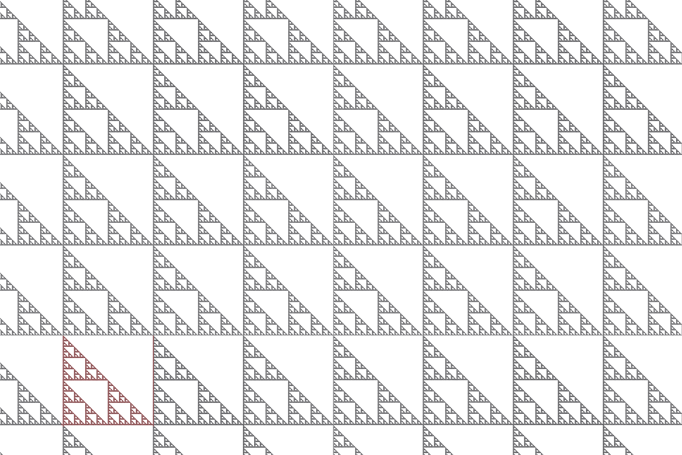
Figure 1. An example of a fast basin of an attractor of an IFS. The attractor of the IFS, a right-angle Sierpinski triangle, is shown in red.

Here the fast basin is

$$\left\{z\in\mathbb{C}:\exists k\in\mathbb{N},(i_{1},i_{2},...,i_{k})\in\{1,2,3\}^{k},f_{i_{1}}\circ f_{i_{2}}\circ...\circ f_{i_{k}}(z)\in A\right\}.$$

In this and other cases, the fast basin is uniquely defined by the attractor $A$, provided that functions of the IFS, the $f_{i}$s, are appropriately analytic. The fast basin is related to the attractor $A$ analogously to the way that analytic continuation of a function is related to its (multivariable) Taylor series expansion about a point. The attractor plays the role of the power series, and the fast basin plays the role of the analytic continuation. This analogy can be made precise for analytic fractal interpolation functions, as explained in [Barnsley & Vince 2].

An example, illustrating the relationship between fast basin and analytic continuation, is provided by the IFS

$$\mathcal{F}_{1}\mathcal{=}\{\mathbb{C\times C};f_{+1+i},f_{-1+i},f_{+1-i},f_{-1-i}\}$$

where

$$f_{\pm 1-i}\begin{pmatrix}z\\ w\end{pmatrix} =\begin{pmatrix}\frac{1}{2}&0\\ \frac{\pm 1-i}{2}&\frac{1}{4}\end{pmatrix}\begin{pmatrix}z\\ w\end{pmatrix}+\begin{pmatrix}\frac{\pm-i}{2}\\ \frac{\mp i}{2}\end{pmatrix};$$

$$f_{\pm 1+i}\begin{pmatrix}z\\ w\end{pmatrix} =\begin{pmatrix}\frac{1}{2}&0\\ \frac{\pm 1+i}{2}&\frac{1}{4}\end{pmatrix}\begin{pmatrix}z\\ w\end{pmatrix}+\begin{pmatrix}\frac{\pm 1+i}{2}\\ \frac{\pm i}{2}\end{pmatrix}.$$

The unique attractor $A_{1}$ of $\mathcal{F}_{1}$ is the graph of $z\mapsto z^{2}$ over the square $-1\leq\operatorname{Re}z,\operatorname{Im}z\leq+1$. The fast basin of $A_{1}$ is the manifold

$$\left\{(z,z^{2})\in\mathbb{C\times C}:z\in\mathbb{C}\right\}.$$

In other words, the fast basin of $A_{1}$ (w.r.t. the IFS $\mathcal{F}_{1}$) is the Riemann surface for $z\mapsto z^{2}$ over $\mathbb{C}$. This manifold can be characterized as the set of points $(z_{0},w_{0})\in$ $\mathbb{C\times C}$ such that there exists $f:\mathbb{C\times C\rightarrow C\times C}$ of the form $f(z,w)=(az+b,F(z,w))$, where $F(z,w)$ is holomorphic and invertible, $F(\mathbb{C\times C)=C}$, $a,b\in\mathbb{C}$, with the properties (i) $f(A_{1})\subset A_{1}$ and   (ii) $f(z_{0},w_{0})\in A_{1}$. The fast basin, in this case, is independent of the analytic IFS that is used to generate it, modulo some natural conditions.

Fast basins are distinct from the ”macrofractals” discussed in [Banakh & Novosad] which include (the union of two isometric copies of) the ”macro-Cantor” set

$$\left\{\sum_{k=0}^{\infty}2x_{k}3^{k}:(x_{k})\in\{0,1\}^{\mathbb{N}}\right\}\text{.}$$

The latter is an asymptotic counterpart of the Cantor set, see [Banakh & Zarichnyi], and also [Dranishnikov & Zarichnyi]. For a contractive IFS on a complete metric space, the ”macrofractal” is the closure of the set of fixed points of the inverse or dual IFS.

In Section 2 we define and discuss IFSs, their (strict) attractors, basins, continuations, and fast basins. We also mention other motivations for this study.

In Section 3 we establish how connectivity, porosity, dimension, and possession of an empty interior, of the attractor are shared with the fractal continuations and the fast basin of the attractor. The main conclusions are summarized in Table 1.

In Section 4 we illustrate examples of fast basins.

In Section 5 we consider the dynamics induced by the IFS on the fast basin of an attractor.

In Section 6 define the slow basin of an attractor of an IFS, and establish some of its basic topological properties. Roughly speaking, the slow basin of an attractor $A$ comprises those points whose $\omega$-limit set under the Hutchinson operator of the IFS has non empty intersection with the attractor. It includes both the basin and the fast basin of an attractor.

2. Definitions

For the purposes of this paper we use the following definition of an IFS.

Definition 1.

An iterated function system (IFS) is a topological space $X$ together with a finite set of homeomorphisms $w_{i}:X\rightarrow X$, $i=1,2,\dots,N$.

We use the notation

(2.1) $$\mathcal{W}=\{X;w_{1},w_{2},...,w_{N}\}$$

to denote an IFS. Other more general definitions of an IFS are used in the literature; for example, the collection of functions in the IFS may be infinite, see for example [Wicks, Kieninger, Arbieto et al], or the functions may themselves be set-valued [Kunze et al, Lasota & Myjak]. However, throughout this paper, $N$ is a finite positive integer and, except where otherwise stated, $X$ is a complete metric space.

The Hutchinson operator $W:\mathcal{K}(X)\rightarrow\mathcal{K}(X)$ is defined on the family of nonempty compact sets $S\in\mathcal{K}(X)$ by $W(S):=\bigcup_{i=1}^{N}w_{i}(S)$. The $k$-fold composition of $W$ is denoted by $W^{k}$ with the convention that $W^{0}$ means the identity map. By the inverse image of $S\subset X$ under $W$ we understand the set

$$W^{-1}(S)=\{x\in X:W(x)\cap S\neq\emptyset\}.$$

This is the large counter-image employed in set-valued analysis, cf. [Aliprantis & Border]. Obviously

$$W^{-1}(S)=\bigcup_{n=1}^{N}w_{n}^{-1}(S),$$

where $w_{n}^{-1}(S)$ is the image of $S$ under the inverse map $w_{n}^{-1}$ or, equivalently, the counter-image of $S$ under $w_{n}$.

Throughout we assume that the IFS $\mathcal{W}$ possesses a strict attractor, $A$. Following [Barnsley & Vince] we recall that a closed set $A\subset X$ is a strict attractor of $\mathcal{W}$, when there exists an open set $B\supset A$ such that $W^{k}(S)\rightarrow A$ for every nonempty compact $S\subset B$, where the set-convergence is meant in the sense of Hausdorff. The maximal open set $B(A)$ with the above property is called the basin of the attractor $A$ (with respect to $\mathcal{W}$). From the definition it follows that $A$ is compact, nonempty and invariant; that is

$$A\in\mathcal{K}(X)\text{, and }W(A)=A\text{;}$$

see for example [Barnsley & Lesniak, Arbieto et al].

We tend to omit the adjective ’strict’ and refer to $A$ briefly as an attractor. However, the reader should be aware that there are other definitions of the notion of an attractor, see for example [Barnsley et al]. It is widely known that strict attractors occur in contractive systems; see [Barnsley, Falconer, Edgar] for discussion of contractive systems as described in Hutchinson’s original paper [Hutchinson], and see [Barnsley & Demko, Hata, Wicks, Mate, Andres & Fiser] for discussion of more general contractive systems. But an IFS which is not contractive can possess a strict attractor, see [Kameyama, Barnsley & Vince, Vince] and also the following simple example.

Example 2.

Let $X$ be a compactum and $h:X\rightarrow X$ be a homeomorphism such that $X$ is a minimal invariant set, i.e., if $S\in\mathcal{K}(X)$ and $h(S)=S$, then $S=X$. By a virtue of the Birkhoff’s minimal invariant set theorem (see [Gottschalk] and references therein) we know that the forward orbit of any point in $X$ under $h$ is dense in $X$,

$$\forall_{x_{0}\in X}\;\overline{\{h^{k}(x_{0}):k\geq 0\}}=X.$$

A canonical situation of this kind arises for an irrational rotation of the circle. The IFS $\mathcal{W=}\{X;e,h\}$, where $e$ is the identity map on $X$, has strict attractor $A=X$ with $B(A)=X$. But this IFS is noncontractive and cannot be remetrized into a system of (weak) contractions. The identity map makes remetrization to a contractive system impossible. Moreover, this is an example of an IFS where the attractor is not point-fibred in the sense of Kieninger (cf. [Kieninger]) and is not topologically self-similar in the sense of Kameyama (cf. [Kameyama]). To see that $X$ is the unique strict attractor of $\mathcal{W}$ we note the following. First, for all $x_{0}\in X$,

$$W^{k}(\{x_{0}\})=\{h^{m}(x_{0}):0\leq m\leq k\}\rightarrow\overline{\{h^{m}(x_{0}):m\geq 0\}}=X.$$

Second, for a general $S\in\mathcal{K}(X)$ we have $W^{k}(S)\rightarrow X$, because $W^{k}(\{x_{0}\})\subset W^{k}(S)\subset X$ for arbitrary $x_{0}\in S$.

For a finite word $(\theta_{1},\theta_{2},\ldots,\theta_{k})\in\{1,{\ldots},N\}^{k}$ we define

$$w_{\theta_{1}..\theta_{k}}:=w_{\theta_{1}}\circ\ldots\circ w_{\theta_{k}}\text{ and }w_{\varnothing}=e\text{,}$$

where $\varnothing$ is the empty (zero-length) word and $e$ is the identity map. Also given an infinite word $\vartheta=(\theta_{1},\ldots,\theta_{k},\ldots)\in\{1,\ldots,N\}^{\infty}$ we write ${\vartheta}|k:=(\theta_{1},\ldots,\theta_{k})\in\{1,\ldots,N\}^{k}$, and we define ${\vartheta}|0:=\varnothing$. Similarly we write

$$w_{{\vartheta}|k}^{-1}:=w_{\theta_{1}}^{-1}\circ\ldots\circ w_{\theta_{k}}^{-1}\text{ and }w_{{\vartheta}|k}^{-1}(S)=\{x\in X:w_{\theta_{k}}\circ\ldots\circ w_{\theta_{1}}(x)\in S\}$$

for all $S\subset X$.

In papers concerning the foundations of IFS theory, and also in dynamical systems theory, basins of attractors are much studied. One reason that basins of attractors are of interest is because they provide examples of sets which are not only simple to describe, either in terms of an algorithm or by specifying the IFS, but also geometrically complicated. The following two examples illustrate this point.

Example 3.

It follows from the work of Vince [Vince] that the basin of an attractor of a Möbius IFS may itself be the complement of an attractor of a different Möbius IFS.

Example 4.

The IFS

$$\mathcal{W}_{\lambda}=\{\widehat{\mathbb{C}};w(z)=z^{2}-\lambda\},$$

where $\lambda\in\mathbb{C}$ and $\widehat{\mathbb{C}}=\mathbb{C\cup\{\infty\}}$, comprises a discrete dynamical system on the Riemann sphere. For $\lambda\in(-0.25,0.75),$ $\mathcal{W}_{\lambda}$ possesses the attractor $A=\{Z_{0}=0.5+\sqrt{1+4\lambda}/2\}$ with basin $B(A)$ which is a simply connected domain bounded by a Jordan curve. In fact, the boundary of $B(A)$, the Jordan curve, is a Julia set. Milnor has illustrated a related example, [Milnor, Figure 1a on p.3-3]. Easy-to-use interactive software that illustrates basins of attractors of $\mathcal{W}_{\lambda}$ is freely available, see for example [iPad].

In this paper we draw attention to the set $\hat{B}$ of those initial conditions $x_{0}\in X$ such that some orbit $x_{k}=w_{\theta_{1}..\theta_{k}}(x_{0})$ intersects the attractor $A$ after a finite number of steps. This set is of interest in the following contexts: (i) analysis on fractals, in connection with ”fractafolds” and ”fractal blow-ups” [Strichartz]; (ii) in connection with a generalization of the notion of analytic continuation, as discussed in Section 1; (iii) in connection with a general framework for understanding fractal tiling [Barnsley & Vince 3]; (iv) in connection with the chaos game algorithm for computing approximations to attractors; (v) in connection with extending fractal transformations (between attractors of pairs of IFSs) to transformations between basins of attractors, [Barnsley & Vince 3].

What is the relationship between $\hat{B}$ and $B(A)$? The examples in Section 4 show that, despite our first impression, there is no direct relation between $\hat{B}$ and $B(A)$ in general.

Definition 5.

A fast basin of the IFS $\mathcal{W}$ with the attractor $A$ is the following set

$$\hat{B}=\{x\in X:\exists_{k{\geq}0}\;W^{k}(x)\cap A\neq\emptyset\}.$$

Definition 6.

A fractal continuation of the attractor $A$ along the infinite word $\vartheta=(\theta_{1},\theta_{2},\ldots)$ is the ascending union

(2.2) $$\hat{B}(\vartheta)=\bigcup_{k{\geq}0}w_{{\vartheta}|k}^{-1}(A).$$

The following observations about the inverse images of the iterations of $W$ clarify and simplify further use of the definitions of the fast basin and fractal continuations.

Lemma 7.

For $S\subset X$

1. $\underbrace{W^{-1}(\ldots(W^{-1}}_{k}(S)\ldots)={(W^{k})}^{-1}(S)$, simply denoted from now on by $W^{-k}(S)$;

2. $W^{-k}(S)=\bigcup_{(\theta_{1},\ldots,\theta_{k})\in\{1,\ldots,N\}^{k}}\;w_{\theta_{1}..\theta_{k}}^{-1}(S)$.

Proposition 8.

There hold the following representations:

1. $\hat{B}(\vartheta)=\{x\in X:\exists_{k\geq 0}\;\;w_{\theta|k}(x)\in A\}$;

2. $\hat{B}=\{x\in X:\exists_{k\geq 0}\;\exists_{(\theta_{1},\ldots,\theta_{k})\in\{1,\ldots,N\}^{k}}\;\;w_{\theta_{1}..\theta_{k}}(x)\in A\}$;

3. $\hat{B}=\bigcup_{k=0}^{\infty}W^{-k}(A)=\bigcup_{\vartheta\in\{1,{\ldots},N\}^{\infty}}\hat{B}(\vartheta)$.

Particularly the descriptive formula

(2.3) $$\hat{B}=\bigcup_{k\geq 0}\;\bigcup_{(\theta_{1},\theta_{2},\ldots,\theta_{k})\in\{1,\ldots,N\}^{k}}\;w_{\theta_{1}..\theta_{k}}^{-1}(A)$$

which follows from combining the above proposition and lemma, shall be useful.

3. Theorems

This is the central section which shows that many properties of the attractor are inherited by its fractal continuations and fast basin. We summarize everything in the common Table 1 (cf. similar tables in [Engelking]).

Table 1. Invariant properties

$A$	$\hat{B}(\vartheta)$	$\hat{B}$
connected	$+$	$+$
pathwise connected	$+$	$+$
boundary set (empty interior)	$+$	$+$
$\sigma$-porous	$+$ $(*)$	$+$ $(*)$
topological (covering) dim $=m$	$+$	$+$
fractal (Hausdorff) dim $=s$	$+$ $(*)$	$+$ $(*)$
$+$ inherits the property from $A$
$(*)$ provided $w_{i}$ are bi-Lipschitz

We start with the property of dimension. By $dim$ we mean either the topological (Čech-Lebesgue covering) dimension or the fractal (Hausdorff-Besicovitch) dimension.

Theorem 9 (Sum theorem for dimension [Engelking, Falconer]).

Let $X$ be a complete metric space and $\{F_{k}\}_{k}$ be a countable family of closed subsets of $X$. Then

$$dim\left(\bigcup_{k}F_{k}\right)=\sup_{k}dim(F_{k}).$$

Theorem 10 (Invariance theorem for dimension [Engelking, Falconer]).

Let $h:X\to X$ be a homeomorphism and $E\subset X$. Then

$$dim(h(E))=dim(E),$$

provided additionally that $w$ is bi-Lipschitz in the case when $dim$ is the Hausdorff dimension.

Theorem 11.

For the attractor $A$ of $\mathcal{W}$, its fractal continuation $\hat{B}(\vartheta)$ along $\vartheta\in\{1,\ldots,N\}^{\infty}$ and the fast basin $\hat{B}$ the formulas

1. $dim(\hat{B}(\vartheta))=dim(A)$,

2. $dim(\hat{B})=dim(A)$

hold true, provided additionally that $w_{i}$ are bi-Lipschitz in the case of the Hausdorff dimension $dim$.

Proof.

Observe that $w_{\vartheta|k}^{-1}$ is a homeomorphism (bi-Lipschitz where necessary), so by the invariance of dimension $dim(A)=dim(w_{\vartheta|k}^{-1}(A))$. Putting now $F_{k}:=w_{\vartheta|k}^{-1}(A))$ for $k\geq 0$ in the sum theorem yields (i) due to (2.2).

In the same way the sum and invariance theorems give (ii) due to (2.3). ∎

Our reasoning considered both cases $\hat{B}$ and $\hat{B}(\vartheta)$ separately because of the two obstacles:

1. the topological dimension in general metric spaces lacks monotonicity, so one cannot exploit the inclusion $A\subset\hat{B}(\vartheta)\subset\hat{B}$;

2. the union representation in Proposition 8 (iii) need not be countable.

Next we study the connectedness of fractal continuations and the fast basin. First note that in the realm of locally compact metric spaces (the class where are build many geometric models) zero-dimensionality is equivalent to hereditary disconnectedness (i.e., lack of connected nonsingleton subsets, a property weaker than the celebrated extreme disconnectedness of the Cantor set). By the de Groot theorem such spaces admit ultrametrization so they have a tree-like structure. Therefore, we get for free from Theorem 11, that whenever the attractor is hereditarily disconnected (has a tree-like structure) the same holds true for its fractal continuations and the whole fast basin. (The above discussion followed [Engelking]).

Theorem 12 (Sum theorem for connectedness [Engelking]).

Let $X$ be a metric space and $\{C_{j}\}_{j}$ be a family of connected (respectively pathwise connected) subsets of $X$ such that $\bigcap_{j}C_{j}\neq\emptyset$. Then the union $\bigcup_{j}C_{j}$ is again connected (respectively pathwise connected).

Theorem 13 (Invariance theorem for connectedness [Engelking]).

Let $h:X\to X$ be a homeomorphism and $E\subset X$ be a connected (respectively pathwise connected) set. Then $h(E)$ is again connected (respectively pathwise connected).

Theorem 14.

If the attractor $A$ of $\mathcal{W}$ is (pathwise) connected, then both its fractal continuation $\hat{B}(\vartheta)$ along $\vartheta\in\{1,\ldots,N\}^{\infty}$ and the fast basin $\hat{B}$ are (pathwise) connected.

Proof.

One needs only to remind that according to (2.2) and (2.3), the sets $\hat{B}$ and $\hat{B}(\vartheta)$ are build from the homeomorphic copies $w_{\theta_{1}..\theta_{k}}^{-1}(A)\supset A$ of $A$, $\theta_{1},\ldots,\theta_{k}\in\{1,\ldots,N\}$, $k\geq 0$, and the intersection of anyhow chosen collection of these copies is nonempty. Hence the invariance and the sum theorem for connectedness give the desired conclusion. ∎

In the end of this section we study how thin/thick attractors affect their continuations and fast basins. Let us recall (cf. [Lucchetti, Zajicek, Barnsley et al]) that a set $S\subset X$ is porous provided

$$\exists_{0<\lambda<1}\;\exists_{r_{0}>0}\;\forall_{s\in S}\;\forall_{0<r<r_{0}}\;\exists_{x\in X}\;N_{{\lambda}r}\{x\}\subset N_{r}\{s\}\setminus S,$$

where $N_{r}\{x\}:=\{y\in X:d(y,x)<r\}$ stands for an open ball. A $\sigma$-porous set is a countable union of porous sets.

Theorem 15.

If the attractor $A$ of $\mathcal{W}$ is thin in one of the following senses:

1. $A$ is $\sigma$-porous,

2. $A$ is boundary (i.e., the interior $intA=\emptyset$),

then both its fractal continuation $\hat{B}(\vartheta)$ along $\vartheta\in\{1,\ldots,N\}^{\infty}$ and the fast basin $\hat{B}$ are thin in the same sense; provided in the case of $\sigma$-porosity that $w_{i}$ are bi-Lipschitz.

Proof.

For (a) it is enough to note that the image of a porous set via bi-Lipschitz homeomorphism (onto the whole space $X$) is again porous.

Part (b) needs the Baire category theorem [Aliprantis & Border]: a countable intersection of dense open sets is dense. We consider only $\hat{B}$ which contains the case $\hat{B}(\vartheta)\subset\hat{B}$. Keep in mind that $h:=w_{\theta_{1}..\theta_{k}}^{-1}$ is a homeomorphism for $\theta_{1},\ldots,\theta_{k}\in\{1,\ldots,N\}$, $k\geq 0$. The sets $X\setminus h(A)$ are open, because $A$ is closed. They are dense, because

$$\overline{X\setminus h(A)}=\overline{h(X\setminus A)}=h(\overline{X\setminus A})=h(X\setminus int(A))=h(X)=X$$

due to the assumption that $int(A)=\emptyset$. By (2.3) we obtain that

$$X\setminus\hat{B}=\bigcap_{k\geq 0}\;\bigcap_{(\theta_{1},\theta_{2},\ldots,\theta_{k})\in\{1,\ldots,N\}^{k}}\;X\setminus w_{\theta_{1}..\theta_{k}}^{-1}(A)$$

is the countable intersection of dense open sets. Hence it is dense, what means exactly that $int(\hat{B})=\emptyset$. ∎

To obtain more properties of the fast basin related to the properties of the attractor one needs to understand better how the ascending sets $W^{-k}(A)$ sit in the fast basin

$$\hat{B}=\bigcup_{k\geq 0}W^{-k}(A).$$

This unavoidably leads to studying the dynamics on the fast basin (Section 5).

4. Examples

We illustrate parts of fast basins.

Figure 2 shows part of the fast basin and, in  red, the attractor of the IFS

(4.1) $$\mathtt{\mathcal{F=\{}}\mathbb{R}^{2};\frac{1}{2}(-y,x),\frac{1}{2}(-y+2,x),\frac{1}{2}(-y,x+2)\}\text{.}$$

(Here we write $(-0.5y,0.5x)$ to mean the function on $\mathbb{R}^{2}$ such that $(x,y)\mapsto(-0.5y,0.5x)$.) The viewing window is $-6.2\leq x,y\leq 6.3$.

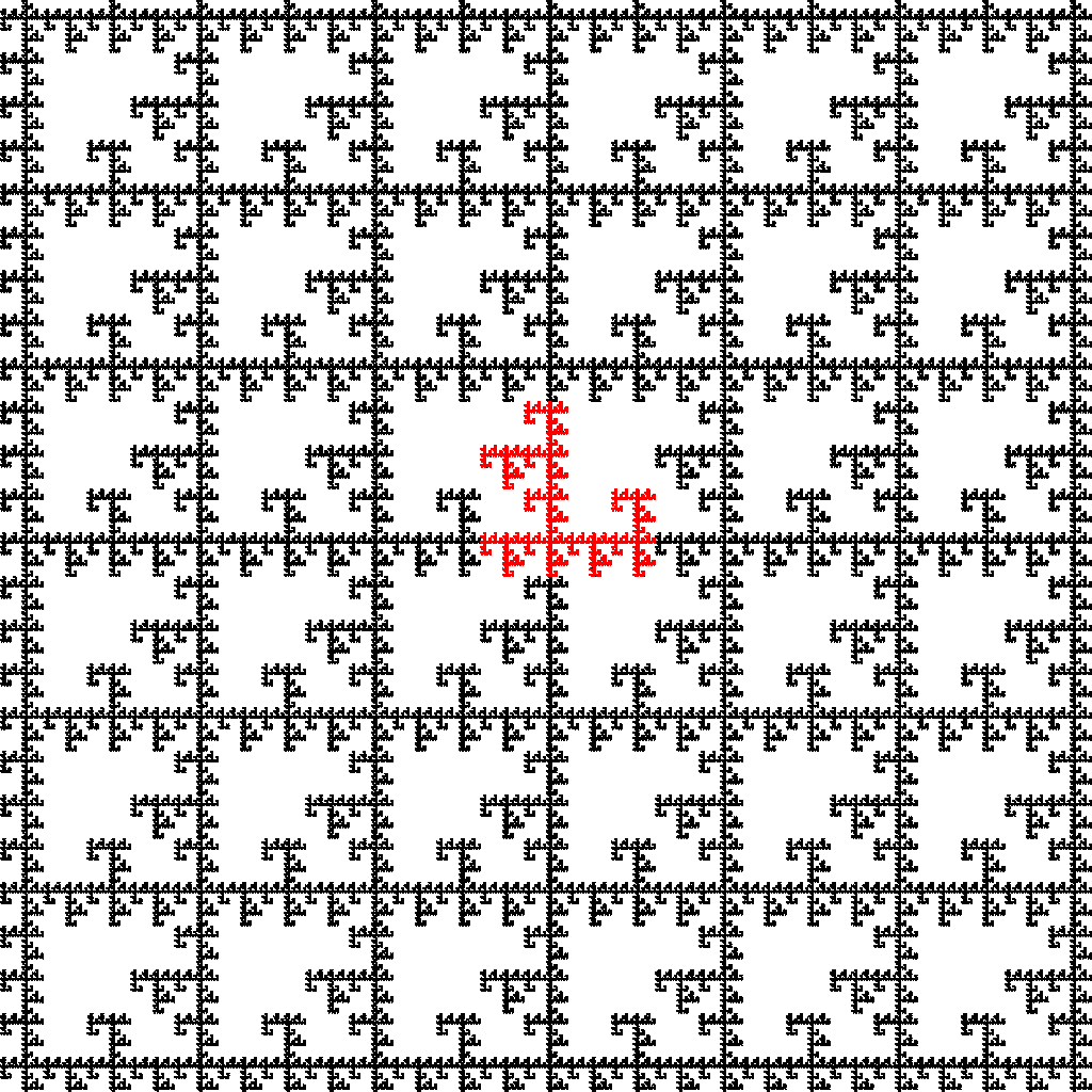
Figure 2. Attractor of the IFS (4.1) and the part of its fast basin within the viewing window. See text.

Figure 3 illustrates a larger region of same fast basin, and colours encode the ”generations” of the fast basin: points in the region in black arrive in four iterations (but in no less number), and so on, as explained in the caption.

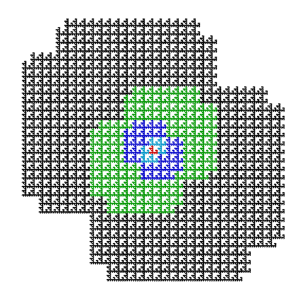
Figure 3. Generations of the fast basin that is also shown in Figure 2. Black points take four (and no less) iterations to arrive on the attractor (red), green points take three (and no less) iterations, dark blue points take two (and no less) and light blue take one iteration.

Fast basin of the Kigami triangle (i.e., the Sierpiński triangle in harmonic coordinates according to [Kigami]).

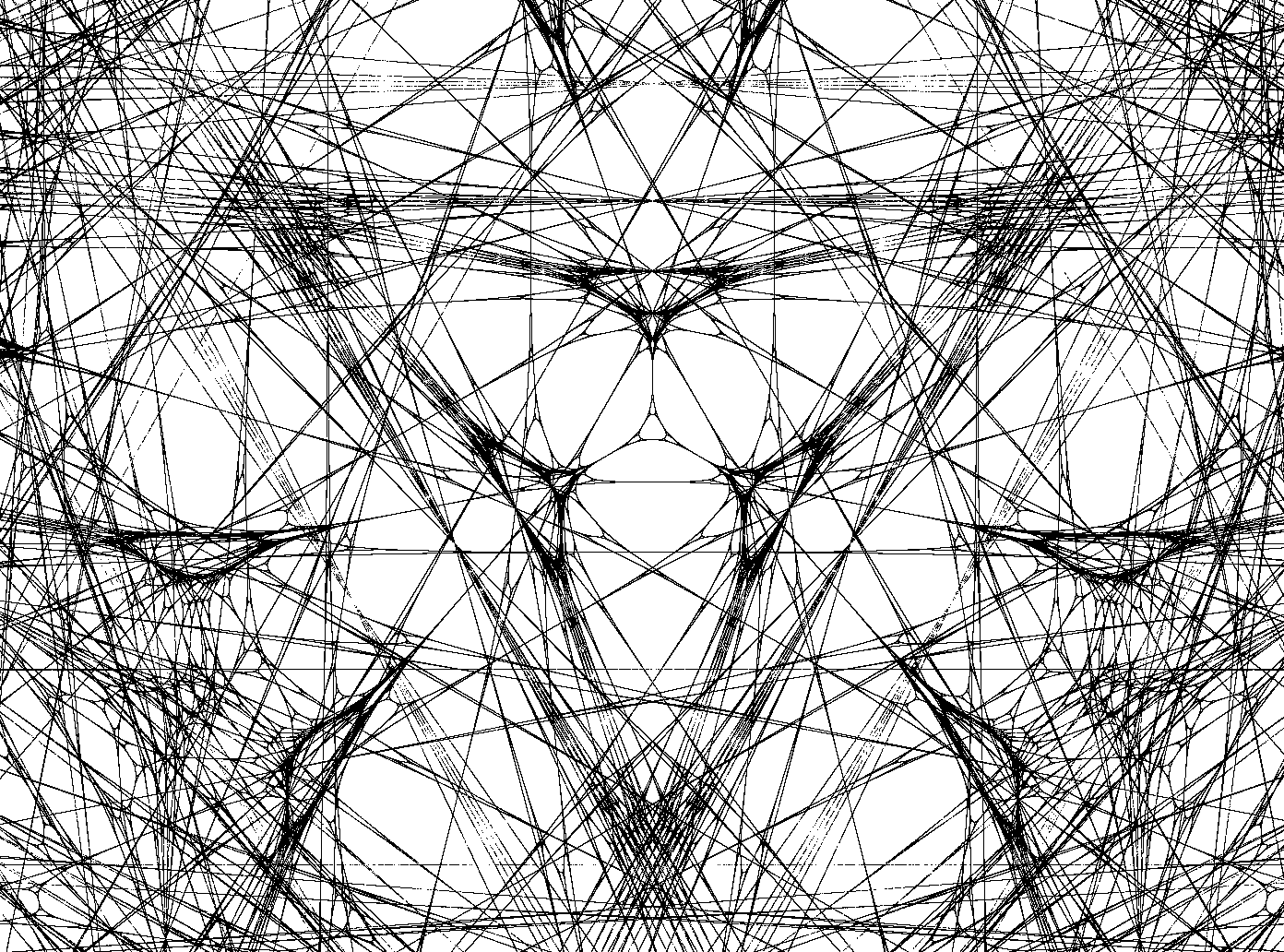
Figure 4. Illustration of part of the fast basin of the Kigami triangle. See text

Figure 4 shows part of the fast basin of Kigami triangle, involving affines rather than similitudes. The IFS is

$$\{\mathbb{R}^{2};\frac{1}{5}(2x+y,x+2y),\frac{1}{5}(3x+2,-x+y+1),\frac{1}{5}(x-y+1,3y+2)\}.$$

The Kigami triangle itself is in the center of the image. In Figure 5 the colours index the ”generations” of the fast basin.

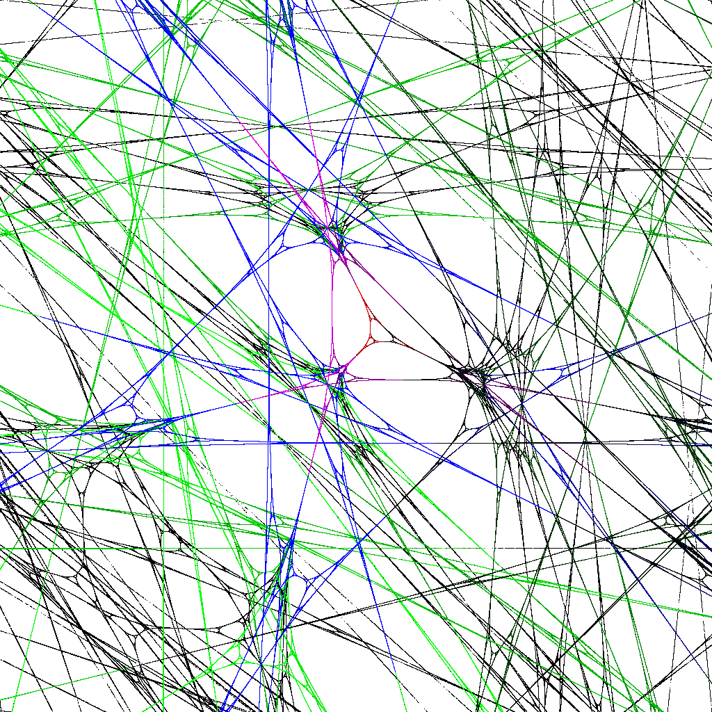
Figure 5. Some of the different ”generations”, in different colours, of the fast basin of the Kigami triangle attractor. See also Figure 4.

A beautiful example of a fast basin is illustrated in Figure 6. The IFS in this case is

$$\{\mathbb{R}^{2};\frac{1}{2}(x,y+1),\frac{1}{2}(-y+1,-x+1),\frac{1}{2}(y+1,-x+1)\}.$$

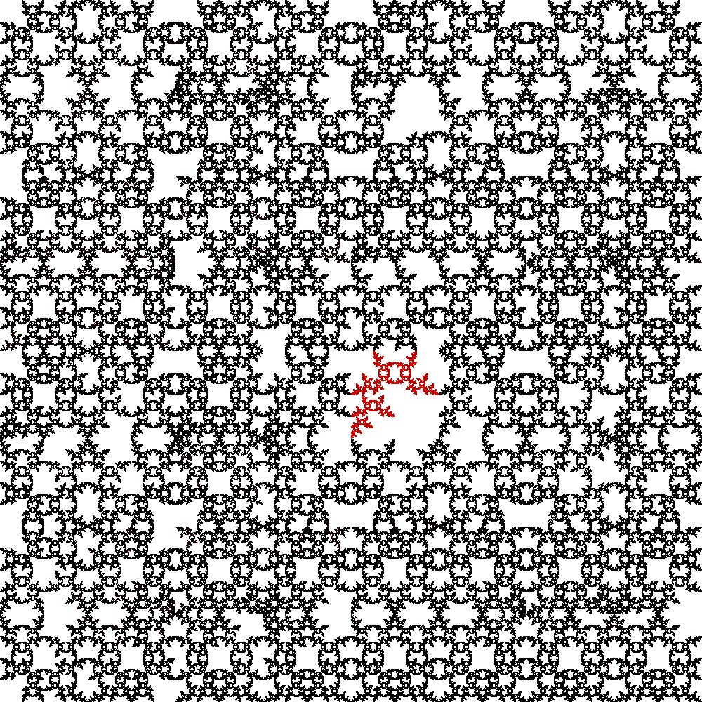
Figure 6. Part of the fast basin associated with the attractor shown in red. See text.

The intricate geometrical complexity of this fast basin contrasts with the algebraic simplicity of the IFS.See also Figure 7.

Figure 7. See text.

Example 16.

(Fast basin reaching outside the basin.) Let $X=\mathbb{R}\cup\{\infty\}$ be the one-point compactification of the real line. Define $w_{1}(x):=x/2$ for $x\neq\infty$, $w_{1}(\infty):=\infty$, and

$$w_{2}(x):=\left\{\begin{array}[c]{ll}\frac{x+3}{6-2x},&x\not\in\{3,\infty\},\\ \infty,&x=3,\\ -\frac{1}{2},&x=\infty.\\ &\end{array}\right.$$

Then $A=[0,1]$ and $\hat{B}\not\subset B(A)$.

Since $w_{1}([0,1])=[0,1/2]$, $w_{2}([0,1])=[1/2,1]$, we have that $A:=[0,1]=W(A)$ is indeed the only candidate for attractor.

The map $w_{1}$ has $0$ as an (exponential) attractor, so we study the behavior of $w_{2}$. Firstly $w_{2}(x)\geq w_{2}(3/2)=3/2$ for $3>x\geq 3/2$, so $[3/2,3)\subset X\setminus B(A)$. Moreover $w_{1}(\infty)=w_{2}(3)=\infty\not\in B(A)$, so $3\not\in B(A)$. Secondly $w_{2}(x)<x$ for $x\in(1,3/2)$. Thirdly $w_{2}(1)=1$ and the derivative $0<w_{2}^{\prime}(x)\leq 3/4$ for $x\leq 1$. Therefore

$$B(A)=\mathbb{R}\setminus[3/2,\infty).$$

Now observe

$$w_{1}^{-n}([3/2,3))=2^{n}\cdot[3/2,3),$$

$$[3/2,\infty)=\bigcup_{n=0}^{\infty}2^{n}\cdot[3/2,3)\subset X\setminus B(A),$$

$$w_{1}^{n+1}(2^{n}\cdot 3)=w_{1}(3/2)=3/4\in A,$$

$$\{3\cdot 2^{n}:n\geq 1\}\subset\hat{B}\setminus B(A).$$

Altogether $\hat{B}\not\subset B(A)$.

5. The dynamics on the fast basin

The first observation expresses how it is ”easy” to escape the fast basin $\hat{B}$ : the orbit of any point not on the fast basin does not meet the fast basin.

Proposition 17.

If $x\not\in\hat{B}$, then $W(x)\cap\hat{B}=\emptyset$.

Proof.

Ad absurdum suppose that some $y=w_{\theta}(x)\in W(x)$, $\theta\in\{1,\ldots,N\}$, falls into $\hat{B}$. Then

$$w_{\theta\theta_{1}..\theta_{k}}(x)=w_{\theta_{1}..\theta_{k}}(y)\in A,$$

which leads to $x\in\hat{B}$. ∎

The next result explains when the fast basin is trivial in terms of the action of the IFS on the attractor.

Proposition 18.

The following are equivalent:

1. $\hat{B}\neq A$,

2. $w_{i}^{-1}(A)\neq A$ for some $i=1,\ldots,N$,

3. $w_{i}(A)\neq A$ for some $i=1,\ldots,N$.

Proof.

Recall that $W^{-1}(A)=\bigcup_{i=1}^{N}\;w_{i}^{-1}(A)$ and $\hat{B}=\bigcup_{k\geq 0}\;W^{-k}(A)$. If $\hat{B}=A$, then $\hat{B}\supset W^{-1}(A)=A$. Conversely, if $W^{-1}(A)=A$, then $W^{-k}(A)=A$ for all $k\geq 0$, so $\hat{B}=A$.

By the invariance of $A$ for all $i=1,\ldots,N$, $w_{i}(A)\subset A$, and so $w_{i}^{-1}(A)\supset A$. Thus $W^{-1}(A)\neq A$ is possible if and only if $w_{i}^{-1}(A)\neq A$ for some $i=1,\ldots,N$. This establishes that (i) and (ii) are equivalent.

Equivalence of (ii) and (iii) is a consequence of the bijectivity of $w_{i}$. ∎

The assumption that the maps $w_{i}$ are homeomorphisms onto the whole space was crucial in the criterion for the fast basin to be nontrivial (cf. the fast basin of the Julia set).

Example 19.

Let $X:=[0,1]\times[1/2,\infty)\subset\mathbb{R}^{2}$ be endowed with the metric induced from the Euclidean distance in the plane. Define $w_{1}(x,y):=(x/2,\sqrt{y})$, $w_{2}(x,y):=(x/2+1/2,\sqrt{y})$, for $(x,y)\in X$. The attractor of $(X;w_{1},w_{2})$ is $A=[0,1]\times\{1\}$. Maps $w_{i}$ are homeomorphisms onto their images $w_{i}:X\to w_{i}(X)$. However $w_{i}(A)\subsetneq A$ despite $w_{i}^{-1}(A)=A$ for $i=1,2$. The fast basin $\hat{B}=A$ is trivial here.

From Proposition 18 we have also an improvement upon Proposition 8 (iii).

Proposition 20.

Let $I:=\{i=1,\ldots,N:w_{i}(A)\subsetneq A\}$ and $\theta_{1},\ldots,\theta_{k}\in\{1,\ldots,N\}$. Then

1. $w_{\theta_{1}..\theta_{k}\sigma}^{-1}(A)\supsetneq w_{\theta_{1}..\theta_{k}}^{-1}(A)$ exactly when $\sigma\in I$,

2. $\hat{B}=\bigcup_{\vartheta\in I^{\infty}}\hat{B}(\vartheta)\cup A$.

Further we consider the reverse dynamics $\mathcal{W}^{-1}:=(\hat{B};w_{1}^{-1},\ldots,w_{N}^{-1})$ on the fast basin. We assume that all $w_{i}^{-1}$ are $L>1$ expansive, i.e.,

$$\forall{y_{1},y_{2}\in X},d(w_{i}^{-1}(y_{1}),w_{i}^{-1}(y_{2}))\geq L\cdot d(y_{1},y_{2}).$$

Moreover we assume that $A$, an attractor of $(X;w_{1},\ldots,w_{N})$, is connected. The reversed dynamics $y_{n}=w_{\theta_{1}...\theta_{n}}^{-1}(y_{0})$ on $\hat{B}$ has two opposite components.

1. Outside big enough disks everything on the fast basin is ”immediately taken away”; there is no ”wandering around”. This is precisely stated in Proposition 22.

2. Given a disk $D\supset A$ around the attractor, we have that the reverse trajectories $y_{n}$ starting at attractor, $y_{0}\in A$, can have arbitrarily large escape from disk times, namely

   (5.1) $$\sup_{y_{1}\neq y_{0}\in A}t(y_{0})=\infty,$$

   where

   $$t(y_{0}):=\sup\{n:\forall_{m\leq n}y_{m}\in D\}.$$

From the above observations it follows that the whole intricate structure of the fast basin is produced nearby the attractor and then flushed into the whole space (look at Figures 4 and 5).

Lemma 21.

For $x_{0}\in X$, $1<\tilde{L}<L$ there exists $r_{0}>0$ s.t. for all $r\geq r_{0}$, $i=1,{\ldots},N$

$$w_{i}^{-1}(X\setminus D(x_{0},r))\subset X\setminus D(x_{0},\tilde{L}r).$$

Proof.

Find $\rho$ s.t. $D(x_{0},\rho)\supset\{w_{i}^{-1}(x_{0}):i=1,{\ldots},N\}$. Next assign $r_{0}:=\rho{/}(L-\tilde{L})$. Thus $\tilde{L}r\leq Lr-\rho$ for $r\geq r_{0}$ and one readily verifies that

$$d(w_{i}^{-1}(x),x_{0})\geq|d(w_{i}^{-1}(x),w_{i}^{-1}(x_{0}))-d(x_{0},w_{i}^{-1}(x_{0}))|>Lr-\rho$$

for $x\not\in D(x_{0},r)$, $i=1,\ldots,N$. ∎

Proposition 22.

Let $x_{0}\in X$, $1<\tilde{L}<L$. Then there exists $r_{0}>0$ s.t. $d(y_{n+m},x_{0})\geq\tilde{L}^{n}\cdot d(y_{m},x_{0})$ whenever $d(y_{m},x_{0})>r_{0}$

Finally we establish (5.1). Define $\delta(a):=d(a,w_{\theta_{1}}^{-1}(a))$ for $a\in A$ and fixed $\theta_{1}$. Put $\Delta(a):=r-d(a,x_{0})$. This controls exits from the disk; namely $y\in D(x_{0},r)$ as long as $d(y,a)\leq\Delta(a)$. Now we track the distance of the reverse trajectory $(y_{n})$ from its starting point $y_{0}:=a\in A$:

$$d(y_{n},y_{0})\leq\sum_{k=0}^{n-1}L^{k}\cdot d(y_{1},y_{0})\leq n\cdot L^{n}\delta(a).$$

To keep the first $n$ points $y_{1},\ldots,y_{n}$ in $D(x_{0},r)$ it is therefore enough to take $a\in A$ such that

$$\delta(a)<\frac{\Delta(a)}{n\cdot L^{n}}.$$

Indeed, $\Delta(a)$ does not vary too much $\|\Delta(a)\|\geq const>0$ for $a$ close to $conv\left(\bigcup_{i=1}^{N}Fix(w_{i})\right)$, and $A\ni a\mapsto\delta(a)$ is a continuous function on the connected set, and $\delta^{-1}(0)=Fix(w_{\theta_{1}})$, so one can find $a\in A$, $y_{1}=w_{\theta_{1}}^{-1}(y_{0})\neq y_{0}=a$, with sufficiently small $\delta(a)$.

6. Slow basin

In the present section we review some basic notation from the theory of hyperspaces as, unlike in the discussion so far, we need to deal with this formalism in a direct way.

Let $x\in X$, $A\subset X$, $r>0$. We shall write

$$d(x,A):=\inf_{a\in A}d(x,a)$$

for the distance from $x$ to $A$,

$$N_{r}A:=\{x\in X:d(x,A)<r\}$$

for the $r$-neighbourhood of $A$, and

$$D_{r}A:=\{x\in X:d(x,A)\leq r\}.$$

for the $r$-dilation of $A$.

We say that a sequence $(x_{n})_{n=1}^{\infty}$ converges to the set $A\subset X$, denoted $x_{n}\to A$, whenever $d(x_{n},A){\to}0$.

Definition 23.

A slow basin of the IFS $\mathcal{W}$ with the attractor $A$ is the following set

$$\tilde{B}=\{x\in X:\exists_{\vartheta\in\{1,\ldots,N\}^{\infty}}\;w_{\vartheta|n}(x)\to A\}.$$

Proposition 24.

The slow basin $\tilde{B}$ contains both the fast basin $\hat{B}$ and the basin $B(A)$ of the attractor $A$.

Proof.

It is enough to check that $B(A)\subset\tilde{B}$. Take $x\in B(A)$ and any $\vartheta\in\{1,\ldots,N\}^{\infty}$. Then

$$d(w_{\vartheta|n}(x),A)\leq\sup\{d(y,A):y\in W^{n}(x)\}\leq d_{H}(W^{n}(x),A){\to}0$$

where $d_{H}$ denotes the Hausdorff distance ([Aliprantis & Border, Beer]). ∎

Lemma 25.

The slow basin is backward (i.e., negatively) invariant: if $x\in\tilde{B}$, then $W^{-1}(x)\subset\tilde{B}$.

Proof.

Let $x\in\tilde{B}$. Then $w_{\vartheta|n}(x)\to A$ for some $\vartheta\in\{1,\ldots,N\}^{\infty}$. Every $y\in W^{-1}(x)$ provides representation $x=w_{\sigma}(y)$ with some $\sigma\in\{1,\ldots,N\}$. Hence

$$w_{\sigma\theta_{1}..\theta_{n}}(y)=w_{\theta_{1}..\theta_{n}}(x)\to A,$$

so $x\in\tilde{B}$. ∎

Theorem 26.

We have the following representations of the slow basin

1. $\tilde{B}=\bigcup_{k\geq 0}W^{-k}(B(A))$,

2. there exists $r_{0}>0$ such that for $0<r<r_{0}$

   $$\tilde{B}=\bigcup_{k\geq 0}W^{-k}(N_{r}A)=\bigcup_{k\geq 0}W^{-k}(D_{r}A).$$

In particular, the slow basin is an open set.

Proof.

Since $B(A)\supset A$ is an open neighbourhood of a compact set, there exists $r_{0}$ such that

$$A\subset N_{r}A\subset D_{r}A\subset N_{r_{0}}A\subset B(A)$$

for $r<r_{0}$. Obviously

$$\tilde{B}\supset\bigcup_{k\geq 0}W^{-k}(B(A))\supset\bigcup_{k\geq 0}W^{-k}(D_{r}A)\supset\bigcup_{k\geq 0}W^{-k}(N_{r}A),$$

$0<r<r_{0}$, due to Lemma 25 and Proposition 24.

Now let $x\in\tilde{B}$. Then $w_{\theta_{1}..\theta_{n}}(x)\to A$ for some $(\theta_{1},\ldots,\theta_{n},\ldots)\in\{1,\ldots,N\}^{\infty}$. From the definition of convergence there exists $k$ such that $w_{\theta_{1}..\theta_{n}}(x)\in N_{r}A$, i.e., $x\in W^{-k}(N_{r}A)$. Therefore $\tilde{B}\subset\bigcup_{k\geq 0}W^{-k}(N_{r}A)$. ∎

Theorem 27.

If $X$ is a space with the property that its open balls are path connected sets, and the attractor $A$ of $\mathcal{W}=(X;w_{1},\ldots,w_{N})$ is connected, then the slow basin $\tilde{B}$ is a path connected set.

Proof.

Since $A$ is connected it is chainable: for each $\varepsilon>0$ and $a_{0},a\in A$ there exists $\{a_{1},\ldots,a_{m}\}\subset A$ with $d(a_{i-1},a_{i})<\varepsilon$, $i=1,\ldots,m$, $a_{m}=a$ (Exercise 3.2.8 (b) p.90 [Beer]). Thus $N_{r}A=\bigcup_{a\in A}N_{r}\{a\}$ is path connected as a connected union of path connected balls.

The sets $w_{i}^{-1}(N_{r}A)$ are homeomorphic images of path connected $N_{r}A$ and form connected union $W^{-1}(N_{r}A)=\bigcup_{i=1}^{N}w_{i}^{-1}(N_{r}A)$, because $w_{i}^{-1}(N_{r}A)\supset w_{i}^{-1}(A)\supset A$.

Inductively all $W^{-k}(N_{r}A)$ are path connected, $k\geq 0$, and $W^{-k}(N_{r}A)\supset A$. This gives path connectedness of $\tilde{B}=\bigcup_{k\geq 0}W^{-k}(N_{r}A)$. ∎

References

- [Aliprantis & Border] Ch.D. Aliprantis, K.C. Border, Infinite Dimensional Analysis: A Hitchhiker’s Guide, Springer 2007.
- [Andres & Fiser] J. Andres, J. Fišer, Metric and topological multivalued fractals, Int. J. Bifurc. Chaos 14 no.4 (2004), 1277–1289.
- [Arbieto et al] A. Arbieto, A. Junqueira, B. Santiago, On weakly hyperbolic iterated functions systems, arXiv:1211.1738, 2012.
- [Banakh & Novosad] T. Banakh, N. Novosad, Micro and macro fractals generated by multi-valued dynamical dystems, arXiv:1304:7529v1, 2013.
- [Banakh & Zarichnyi] T. Banakh, I. Zarichnyi, Characterizing the Cantor bi-cube in asymptotic categories, Groups, Geometry, and Dynamics, 5:4 (2011) 691-728
- [Barnsley] M. F. Barnsley, Fractals Everywhere, Academic Press, 1988; 2nd Edition, Morgan Kaufmann 1993; 3rd Edition, Dover Publications, 2012.
- [Barnsley & Demko] M.F. Barnsley, S. Demko, Iterated function systems and the global construction of fractals, Proc. R. Soc. London Ser. A 399 (1985), 243–275.
- [Barnsley & Lesniak] M.F. Barnsley, K. Leśniak, On the continuity of the Hutchinson operator, arXiv:1202.2485 (preprint)
- [Barnsley et al II] M.F. Barnsley, K. Leśniak, A. Vince, Symbolic iterated function systems, fast basins and fractal manifolds, arXiv:1308.3819v1 [math.DS] (2013)
- [Barnsley & Vince] M.F. Barnsley, A. Vince, Real projective iterated function systems, J. Geom. Anal. 22 (2012), no. 4, 1137–1172.
- [Barnsley & Vince 2] M.F. Barnsley, A. Vince, Fractal continuation of analytic (fractal) functions, arXiv:1209.6100 (preprint), Constructive Approximation, 2013, in press.
- [Barnsley & Vince 3] M.F. Barnsley, A. Vince, Fractal tiling, in preparation (2013).
- [Barnsley et al] M.F. Barnsley, D.C. Wilson, K. Leśniak, Some recent progress concerning topology of fractals, in: K.P. Hart, P. Simon, J. van Mill (Eds.), Recent Progress in General Topology III, Springer 2013.
- [Beer] G.A. Beer, Topologies on closed and closed convex sets, Kluwer 1993.
- [Dranishnikov & Zarichnyi] A. Dranishnikov, M. Zarichnyi, Universal spaces for asymptotic dimension, Topology Applications 140:2-3 (2004), 203–225.
- [Engelking] R. Engelking, General Topology, Helderman, Berlin 1989.
- [Edgar] G. Edgar, Measure, Topology, and Fractal Geometry, Second Edition, Springer 2008.
- [Falconer] K. Falconer, Fractal Geometry: Mathematical Foundations and Applications, Second Edition, Wiley 2003.
- [Gottschalk] W. H. Gottschalk, Minimal sets; an introduction to topological dynamics, Bull. Amer. Math. Soc.64, no.6, (1958), 336–351.
- [Hata] M. Hata, On the structure of self-similar sets, Japan J. Appl. Math. 2 (1985), 381–414.
- [Hutchinson] J. Hutchinson, Fractals and self-similarity, Indiana Univ. Math. J. 30 (1981) 713–747.
- [iPad] Fractile (a Julia set and Mandelbrot set calculator for the iPad and iPhone) www.fractile.net
- [Kameyama] A. Kameyama, Distances on topological self-similar sets and the kneading determinants, J. Math. Kyoto Univ. 40-4 (2000), 603–674.
- [Kieninger] B. Kieninger, Iterated Function Systems on Compact Hausdorff Spaces, Ph.D. Thesis, Augsburg University, Berichte aus der Mathematik, Shaker-Verlag, Aachen 2002.
- [Kigami] J. Kigami, Analysis on fractals, Cambridge University Press 2001.
- [Kunze et al] H. E. Kunze, D. La Torre, E. R. Vrscay, Contractive multifunctions, fixed point inclusions and iterated multifunction systems, J. Math. Anal. Appl. 330 (2007) 159–173.
- [Lasota & Myjak] A. Lasota, J. Myjak, Attractors of multifunctions, Bulletin of the Polish Academy of Sciences, 48 no. 3 (2000) 319–334.
- [Lucchetti] R. Lucchetti, Convexity and Well-Posed Problems, Springer 2006.
- [Mate] L. Máté, The Hutchinson-Barnsley theory for certain noncontraction mappings, Period. Math. Hungar. 27 no.1 (1993), 21–33.
- [Milnor] J. Milnor, Dynamics in One Complex Variable: Introductory Lectures, F. Vieweg&Son, 1999.
- [Strichartz] R.S. Strichartz, Fractafolds based on the Sierpiński gasket and their spectra, Trans. Amer. Math. Soc. 355 (2003), no.10, 4019–4043.
- [Vince] A. Vince, Möbius iterated functions systems, Trans. Amer. Math. Soc. 365 (2013), 491–509.
- [Wicks] K.R. Wicks, Fractals and hyperspaces, Springer 1993.
- [Zajicek] L. Zajíček, On -porous sets in abstract spaces, Abstr. Appl. Anal. (2005), no. 5, 509–534.