The Ginzburg-Landau order parameter near the second critical field

Abstract.

In Ginzburg-Landau theory of superconductivity, the density and location of the superconducting electrons are measured by a complex-valued wave function, the order parameter. In this paper, when the intensity of the applied magnetic field is close to the second critical field, and when the order parameter minimizes the Ginzburg-Landau functional defined over a two dimensional domain, the leading order approximation of its $L^{2}$-norm in ‘small’ squares is given as the Ginzburg-Landau parameter tends to infinity.

1. Introduction

In this paper, we study the minimizers of the Ginzburg-Landau functional of superconductivity. In a two bounded and dimensional simply connected domain $\Omega$ with smooth boundary, the functional is defined over configurations $(\psi,\mathbf{A})\in H^{1}(\Omega;\mathbb{C})\times H^{1}(\Omega;\mathbb{R}^{2})$ as follows,

$$\mathcal{E}(\psi,\mathbf{A}) =\int_{\Omega}e_{\kappa,H}(\psi,\mathbf{A})\,dx$$

$$=\int_{\Omega}\left(|(\nabla-i\kappa H\mathbf{A})\psi|^{2}-\kappa^{2}|\psi|^{2}+\frac{\kappa^{2}}{2}|\psi|^{4}+(\kappa H)^{2}|\operatorname{curl}\mathbf{A}-1)|^{2}\right)\,\,{\rm d}x\,.$$ (1.1)

The modulus of the wave function $\psi$ measures the density of the superconducting electrons; the curl of the vector field $\mathbf{A}$ measures the induced magnetic field; the parameter $H$ measures the intensity of the external magnetic field and the paramter $\kappa$ is a characteristic of the superconducting material. The functional in (1) is invariant under gauge transformations, i.e. if $\chi\in H^{1}(\Omega;\mathbb{R})$, then

$$\mathcal{E}\left(e^{i\chi}\psi,\mathbf{A}+\nabla\chi\right)=\mathcal{E}(\psi,\mathbf{A})\,.$$

The ground state energy of the functional in (1) is,

$$\mathrm{E}_{\rm gs}(\kappa,H)=\inf\{\mathcal{E}(\psi,\mathbf{A})~{}:~{}(\psi,\mathbf{A})\in H^{1}(\Omega;\mathbb{C})\times H^{1}(\Omega;\mathbb{R}^{2})\}\,.$$ (1.2)

The behavior of the ground state energy $\mathrm{E}_{\rm gs}(\kappa,H)$ and of the minimizers depend strongly on the intensity of the external field [7, 15]. Loosely speaking, there exist three critical values $H_{C_{1}}(\kappa)$, $H_{C_{2}}(\kappa)$ and $H_{C_{3}}(\kappa)$ such that, when the parameter $\kappa$ is sufficiently large and $(\psi_{\kappa,H},\mathbf{A}_{\kappa,H})$ is a minimizer of the functional in (1), the following is true:

• If the parameter $H$ satisfies $H<H_{C_{1}}$, then $|\psi_{\kappa,H}|>0$ everywhere;

• if $H_{C_{1}}<H<H_{C_{2}}$, then $|\psi_{\kappa,H}|$ has isolated zeros, called vortices; these zeros become evenly distributed in the domain $\Omega$ when $H\gg H_{C_{1}}$;

• if $H_{C_{2}}<H<H_{C_{3}}$, $|\psi_{\kappa,H}|$ is localized near the boundary of the domain $\Omega$ (this is the surface superconductivity regime);

• if $H>H_{C_{3}}$, $|\psi_{\kappa,H}|=0$ everywhere.

The two monographs [7] and [15] are completely devoted to the detailed analysis of the critical fields in the large $\kappa$ regime, i.e. $\kappa\to\infty$. The regime where vortices exist (i.e. $H<H_{C_{2}}$) is analyzed in [15]. The regime of surface superconductivity above $H_{C_{2}}$ is the subject of [7].

A useful way to distinguish between the various critical fields is the analysis of the distribution of the energy density in the domain ($e_{\kappa,H}(\psi,\mathbf{A})$ in (1)). This is used in [14] to distinguish the surface behavior above $H_{C_{2}}$ and in [16] to study the bulk behavior below $H_{C_{2}}$.

As a consequence of the results in [14], a minimizing order parameter $\psi$ is localized near the boundary of the domain and exhibits a boundary layer with a length scale of order $\kappa^{-1}$. This behavior is valid when $H_{C_{2}}<H<H_{C_{3}}$. The result of [14] is sharpened in [5] and [6].

The results of [16] are valid when the magnetic field is comparable with the critical field $H_{C_{2}}$ and $H<H_{C_{2}}$. It is obtained that the energy density is uniformly distributed in the bulk of the domain thereby suggesting periodicity of minimizing order parameters.

In this paper, we investigate the behavior of the minimizers when $H$ is close to and below the critical value $H_{C_{2}}$. Existing mathematical results [3, 4, 11, 14, 16] suggest that

$$H_{C_{2}}(\kappa)=\kappa+o(\kappa)\quad{\rm as~{}}\kappa\to\infty\,.$$

In [11], when the parameter $H$ satisfies

$$H=\kappa+o(\kappa)\,,\quad(\kappa\to\infty)\,,$$

it is obtained the following formula for the ground state energy,

$$\mathrm{E}_{\rm gs}(\kappa,H)=E_{\rm surf}|\partial\Omega|\kappa+E_{\rm Ab}|\Omega|\,[\kappa-H]^{2}_{+}+o\Big{(}\max\big{(}\kappa,[\kappa-H]^{2}_{+}\big{)}\Big{)}\,,\quad(\kappa\to\infty)\,.$$ (1.3)

Here $E_{\rm surf}<0$ and $E_{\rm Ab}<0$ are two universal constants, of which $E_{\rm Ab}$ is related to the celebrated Abrikosov energy [1]; $|\partial\Omega|$ is the arc-length measure of the boundary and $|\Omega|$ is the Lebesgue (area) measure of $\Omega$.

The asymptotics in (1.3) displays the transition from bulk to surface concentration of the energy close to the critical field $H_{C_{2}}$. It says little about the concentration of minimizing order parameters. If $(\psi,\mathbf{A})$ is a minimizer of the functional in (1), then it follows from (1.3),

$$\int_{\Omega}|\psi|^{4}\,dx=-\frac{2E_{\rm surf}}{\kappa}|\partial\Omega|-2E_{\rm Ab}\,\left[1-\frac{H}{\kappa}\right]_{+}^{2}|\Omega|+o\left(\max\Big{(}\frac{1}{\kappa},\left[1-\frac{H}{\kappa}\right]^{2}_{+}\Big{)}\right)\,,\quad(\kappa\to\infty)\,.$$ (1.4)

Clearly, if the parameter $H$ satisfies  $\kappa^{-1/2}\ll 1-\frac{H}{\kappa}\ll 1$, then the bulk term in (1.4) is the dominant term. In this case, (1.4) is compatible with the following $L^{\infty}$-bound obtained in [11],

$$\|\psi\|_{L^{\infty}(\Omega_{\kappa,\rho})}\leq C\left[1-\frac{H}{\kappa}\right]^{1/2}\,,$$ (1.5)

where $\Omega_{\kappa,\rho}=\{x\in\Omega~{}:~{}{\rm dist}(x,\partial\Omega)\geq\kappa^{-1+\rho}\}$, $\rho\in(0,1)$ and $C$ is a constant. In this paper we establish the additional asymptotics of $|\psi|^{2}$,

$$\int_{\Omega}|\psi|^{2}\,dx=-2{E_{\rm Ab}}\,\left[1-\frac{H}{\kappa}\right]|\Omega|+o\left(\left[1-\frac{H}{\kappa}\right]\right)\,,\quad(\kappa\to\infty)\,.$$ (1.6)

The asymptotics in (1.6) seems more relevant to physicists than the one in (1.4). The density of superconducting electrons (Cooper pairs) is proportional to $|\psi|^{2}$. Consequently, (1.6) tells us what the average of the density of Cooper pairs in $\Omega$ is. Furthermore, the right side of (1.6) displays the intensity of bulk superconductivity, and describes how fast superconductivity is restored in the sample when the magnetic field is gradually decreased.

The precise statement of the main result of this paper is:

Theorem 1.1.

Suppose that $H$ is a function of $\kappa$, $H<\kappa$ and

$$\kappa^{-1/2}\ll 1-\frac{H}{\kappa}\ll 1\,,\quad(\kappa\to\infty)\,.$$

Let $R_{0}>0$, $R_{1}>0$, $\rho\in(0,1)$ and $Q_{\ell}$ be a square of side length $\ell$ such that,

$$Q_{\ell}\subset\{x\in\Omega~{}:~{}{\rm dist}(x,\partial\Omega)\geq\kappa^{-1+\rho}\}\,,$$

$\ell$ a function of $\kappa$, $\displaystyle\frac{\ell^{2}\kappa H}{2\pi}\in\mathbb{N}$ and $R_{0}\kappa^{-1/2}\leq\ell\leq R_{1}\kappa^{-1/4}$ for all $\kappa$.

If $(\psi,\mathbf{A})$ is a minimizer of the functional in (1), then,

$$\frac{1}{|Q_{\ell}|}\int_{Q_{\ell}}|\psi|^{2}\,dx=-2E_{\rm Ab}\left[1-\frac{H}{\kappa}\right]+o\left(\left[1-\frac{H}{\kappa}\right]\right)\,,\quad(\kappa\to\infty)\,.$$ (1.7)

Here $E_{\rm Ab}\in\,[-\frac{1}{2},0[$ is a universal constant defined in (3.17).

A key step to prove Theorem 1.1 is the approximation of the order parameter $\psi$ by a periodic eigenfunction of the Landau Hamiltonian (see Theorem 4.5). In [4], such an approximation is given when $\kappa$ and $H$ satisfy,

$$\kappa^{-2/5}\ll 1-\frac{H}{\kappa}\ll\frac{1}{(\ln\kappa)^{2}}\,,\quad(\kappa\to\infty)\,.$$

This assumption is restrictive compared to that of Theorem 1.1. Furthermore, the result of Theorem 1.1 goes beyond the result of [4] as the formula (1.7) is new.

Thanks to the sharp $L^{\infty}$ bound in (1.5), we have the following slight improvements of Theorem 1.1. If the side length of the square $Q_{\ell}$ satisfies the relaxed condition $R_{0}\kappa^{-1/2}\leq\ell\ll 1$, then it can be approximated by squares of side length satisfying the condition of Theorem 1.1 and the asymptotics in (1.7) remains true. The same remark applies if the square $Q_{\ell}$ is replaced by a domain that can be approximated by squares whose side lengths satisfy the condition in Theorem 1.1. In particular, if squares in Theorem 1.1 are replaced by disks of radii $\ell$ or parallelograms of side lengths comparable with $\ell$, then the asymptotics in (1.7) remains true.

The condition made on the side-length $\ell$, namely $\ell\geq R_{0}\kappa^{-1/2}$, is technical. It is needed to get that the remainder terms of the estimates in Propositions 4.1 and 4.2 are of lower order compared to the expected leading order term. The method we use to approximate the energy implies that the asymptotics in Theorem 1.1 is true if and only if one can select $\delta\in(0,1)$ and $\ell\in(0,1)$ such that,

$$\delta^{-1}\ell^{2}\kappa+\delta\kappa+\ell^{-1}\ll[\kappa-H]\,.$$ (1.8)

Clearly, we observe that the condition $\ell\geq R_{0}\kappa^{-1/2}$ may be relaxed down to $\ell\gg\kappa^{-1}$ if we know that $1-\frac{H}{\kappa}$ is not close to $\kappa^{-1/2}$. More precisely, if $1\ll h(\kappa)\ll\kappa^{1/2}$, $\delta=\left(h(\kappa)\left(1-\frac{H}{\kappa}\right)\kappa^{-1}\right)^{1/2}$ and

$$\frac{1}{h(\kappa)}\ll 1-\frac{H}{\kappa}\ll 1\,,$$

then the asymptotics in Theorem 1.1 remains true for $\ell=h(\kappa)\kappa^{-1}$.

There might be a physically relevant reason behinds the technical point that forces $\ell$ to increase up to the order of $\kappa^{-1/2}$ when $1-\frac{H}{\kappa}$ approaches $\kappa^{-1/2}$. In [16], when $H$ is below but not asymptotically close to $H_{C_{2}}$, it is constructed test configurations that hint at the expected behavior of minimizers. As a consequence, it is expected that the minimizing order parameter will have vortices and the core size of each vortex is proportional to $\kappa^{-1}$. As $H$ approaches $H_{C_{2}}\sim\kappa$, the core size of the vortex might increase up to $\kappa^{-1/2}$. When $H$ is increased further up to $\kappa-\mu\sqrt{\kappa}$ and $\mu\ll 1$, it is expected that all vortices will merge into a giant vortex and superconductivity becomes a surface phenomenon, as is revealed from the energy asymptotics in (1.3). However, the rigorous verification of the aforementioned picture is open.

It is not likely that the result of Theorem 1.1 extends to squares $Q_{\ell}$ that live at a distance of order $\kappa^{-1}$ away from the boundary $\partial\Omega$. It is pointed in [14] that minimizing order parameters will be of order $1$ in a boundary layer of length scale $\kappa^{-1}$.

There is an interesting consequence of Theorem 1.1. If we know that $E_{\rm Ab}=-\frac{1}{2}$, then (1.4) and (1.6) together yield,

$$\lim_{\kappa\to\infty}\int_{\Omega}\big{(}A-|u|^{2}\big{)}^{2}\,dx=0\,,\quad A=-2E_{\rm Ab}\,,\quad u=\left[1-\frac{H}{\kappa}\right]^{-1/2}\psi\,.$$ (1.9)

Such a bound is helpful to construct a vortex structure of $u$ [15]. However, if $-\frac{1}{2}<E_{\rm Ab}<0$, a convergence such as the one in (1.9) does not hold and the profile of $|\psi|^{2}$ is not homogeneous a.e. in $\Omega$. Existing estimates suggest that $E_{\rm Ab}<-\frac{1}{2}$ (see [2, 17]) which rule out the complete homogeneity of $|\psi|^{2}$. Notice that this is in agreement with the expected behavior that $\psi$ will have isolated zeros arranged in a (triangular) lattice, [1].

We conclude by clarifying some notation that will be used throughout this paper. If $a(\kappa)$ and $b(\kappa)$ are two positive functions, we write $a(\kappa)\approx b(\kappa)$ to mean that there exist positive constants $\kappa_{0}$, $c_{1}$ and $c_{2}$ such that $c_{1}b(\kappa)\leq a(\kappa)\leq c_{2}b(\kappa)$ for all $\kappa\geq\kappa_{0}$. The notation $a(\kappa)\sim b(\kappa)$ means that $a(\kappa)=b(\kappa)\big{(}1+o(1)\big{)}$ as $\kappa\to\infty$. The notation $a(\kappa)\ll b(\kappa)$ means $a(\kappa)=o(1)\,b(\kappa)$ as $\kappa\to\infty$. Constants in the remainder of inequalities are all denoted by the letter $C$, whose value might change from a line to another.

Finally, notice that in the parameter regime of Theorem 1.1,

$$\left[1-\frac{H}{\kappa}\right]=\left[\frac{\kappa}{H}-1\right]\big{(}1+o(1)\big{)}\,,\quad(\kappa\to\infty)\,.$$

This remark will be often used throughout the paper.

2. Useful estimates

In this section, we collect a priori estimates satisfied by critical points of the functional in (1). Notice that critical points of the functional in (1) satisfy the Ginzburg-Landau equations:

$$\left\{\begin{array}[]{l}-(\nabla-i\kappa H\mathbf{A})^{2}\psi=\kappa^{2}(1-|\psi|^{2})\psi\,,\\ -\nabla^{\bot}\operatorname{curl}\mathbf{A}=(\kappa H)^{-1}{\rm Im}(\overline{\psi}\,(\nabla-i\kappa H\mathbf{A})\psi)\,,\quad{\rm in}~{}\Omega\,,\\ \nu\cdot(\nabla-i\kappa H\mathbf{A})\psi=0\,,\quad\operatorname{curl}\mathbf{A}=1\,,\quad{\rm on}~{}\partial\Omega\,.\end{array}\right.$$ (2.1)

Here $\nu$ is the unit inward normal vector of $\partial\Omega$. The set of estimates in Lemma 2.1 appeared first in [13] (for a more particular regime) and were then proved for a wider regime in [9].

Lemma 2.1.

There exist positive constants $\kappa_{0}$ and $C$ such that, if $\kappa\geq\kappa_{0}$, $H\geq\frac{\kappa}{2}$ and $(\psi,\mathbf{A})$ is a solution of (2.1), then,

$$\|\operatorname{curl}\mathbf{A}-1\|_{C^{1}(\Omega)}+\kappa^{-1}\|\operatorname{curl}\mathbf{A}-1\|_{C^{2}(\Omega)}\leq C\kappa^{-1}\,,$$ (2.2)

$$\|(\nabla-i\kappa H\mathbf{A})\psi\|_{L^{\infty}(\Omega)}\leq C\kappa\,.$$ (2.3)

The sharp $L^{\infty}$ bound in the next theorem is established in [11]. It has been conjectured in a weaker form in [3]. The bound of Theorem 2.2 plays a key-role in the proof of Theorem 1.1.

Theorem 2.2.

Let $\rho\in(0,1)$. Suppose that $\kappa$ and $H$ satisfy,

$$\kappa^{-1/2}\ll 1-\frac{H}{\kappa}\ll 1\,,\quad(\kappa\to\infty)\,.$$

There exist positive constants $C>0$ and $\kappa_{0}$ such that, if $\kappa\geq\kappa_{0}$ and $(\psi,{\bf A})$ is a solution of (2.1), then,

$$\|\psi\|_{L^{\infty}(\Omega_{\kappa,\rho})}\leq C\left[1-\frac{H}{\kappa}\right]^{1/2}\,,$$ (2.4)

where

$$\Omega_{\kappa,\rho}:=\{x\in\Omega\,|\,\operatorname{dist}(x,\partial\Omega)\geq\kappa^{-1+\rho}\}\,.$$ (2.5)

3. The limiting problem

3.1. Reduced Ginzburg-Landau functional

Given a constant $b\geq 0$ and an open set $\mathcal{D}\subset\mathbb{R}^{2}$, we define the following Ginzburg-Landau energy,

$$G_{b,\mathcal{D}}(u)=\int_{\mathcal{D}}\left(b|(\nabla-i\mathbf{A}_{0})u|^{2}-|u|^{2}+\frac{1}{2}|u|^{4}\right)\,dx\,.$$ (3.1)

Here $\mathbf{A}_{0}$ is the canonical magnetic potential with unit constant magnetic field,

$$\mathbf{A}_{0}(x_{1},x_{2})=\frac{1}{2}(-x_{2},x_{1})\,,\quad\Big{(}x=(x_{1},x_{2})\in\mathbb{R}^{2}\Big{)}\,.$$ (3.2)

We will consider the functional $G_{b,\mathcal{D}}$ first with Dirichlet and later with (magnetic) periodic boundary conditions. It will be clear from the context what is meant.

Consider the functional with Dirichlet boundary conditions and for $b>0$. If the domain $\mathcal{D}$ is bounded, completing the square in the expression of $G_{b,\mathcal{D}}$ shows that $G_{b,\mathcal{D}}$ is bounded from below. Thus, starting from a minimizing sequence, it is easy to check that $G_{b,\mathcal{D}}$ has a minimizer. A standard application of the maximum principle shows that, if $u$ is any minimizer of $G_{b,\mathcal{D}}$, then

$$|u|\leq 1,\qquad\text{ in }{\mathcal{D}},$$ (3.3)

see e.g. [15].

Given $R>0$, we denote by $K_{R}=(-R/2,R/2)\times(-R/2,R/2)$ a square of side length $R$. Let,

$$m_{0}(b,R)=\inf_{u\in H^{1}_{0}(K_{R};\mathbb{C})}G_{b,K_{R}}(u)\,.$$ (3.4)

The following remark will be useful. If $u_{R}$ is a minimizer of (3.4), then $u_{R}$ satisfies the Ginzburg-Landau equation,

$$-(\nabla-i\mathbf{A}_{0})^{2}u_{R}=b^{-1}(1-|u_{R}|^{2})u_{R}\,,\quad{\rm in~{}}Q_{R}\,.$$

Recall that $u_{R}\in H^{1}_{0}(Q_{R})$. We extend $u_{R}$ by magnetic periodicity to all $\mathbb{R}^{2}$, i.e. to a function in the space $E_{R}$ in (3.6) below. That way, $u_{R}$ satisfies the equation

$$-(\nabla-i\mathbf{A}_{0})^{2}u_{R}=b^{-1}(1-|u_{R}|^{2})u_{R}\,,$$

in all $\mathbb{R}^{2}$. We can apply Theorem 3.1 in [8] to get that,

$$\forall~{}b\in[1-b_{0},1[\,,\quad|u_{R}|\leq C_{\max}\sqrt{1-b}\,,$$ (3.5)

where $b_{0}$ and $C_{\max}$ are universal constant.

3.2. Periodic minimizers

We introduce the following space,

$$E_{R}=\bigg{\{}u\in H^{1}_{\rm loc}(\mathbb{R}^{2};\mathbb{C})~{}:~{}u(x_{1}+R,x_{2})=e^{iRx_{2}/2}u(x_{1},x_{2}),\\ u(x_{1},x_{2}+R)=e^{-iRx_{1}/2}u(x_{1},x_{2})\,,~{}\Big{(}(x_{1},x_{2})\in\mathbb{R}^{2}\Big{)}\bigg{\}}\,.$$ (3.6)

Notice that the periodicity conditions in (3.6) are constructed in such a manner that all physically relevant quantities are periodic (i.e. density, energy and super-current). More precisely, for any function $u\in E_{R}$, the functions $|u|$, $|\nabla_{\mathbf{A}_{0}}u|$ and the vector field $\overline{u}\nabla_{\mathbf{A}_{0}}u$ are periodic with respect to the lattice generated by $K_{R}$.

Recall the functional $G_{b,\mathcal{D}}$ in (3.1) above. We introduce the ground state energy,

$$m_{\rm p}(b,R)=\inf_{u\in E_{R}}G_{b,K_{R}}(u)\,.$$ (3.7)

The next proposition exhibits a relation between the ground state energies $m_{0}(b,R)$ and $m_{\rm p}(b,R)$, namely that $m_{\rm p}(b,R)$ is a valid approximation of $m_{0}(b,R)$ when $[1-b]R\ll 1$. It is proved in [10].

Proposition 3.1.

Let $m_{0}(b,R)$ and $m_{\rm p}(b,R)$ be as introduced in (3.4) and (3.7) respectively. For all $b>0$ and $R>0$, we have,

$$m_{0}(b,R)\geq m_{\rm p}(b,R)\,.$$

Furthermore, there exist universal constants $\epsilon_{0}\in(0,1)$ and $C>0$ such that, if $b\geq 1-\epsilon_{0}$ and $R\geq 2$, then,

$$m_{0}(b,R)\leq m_{\rm p}(b,R)+C[1-b]_{+}R\,.$$ (3.8)

3.3. The periodic Schrödinger operator with constant magnetic field.

In this section, we assume the quantization condition that $|K_{R}|/(2\pi)$ is an integer, i.e. there exists $N\in\mathbb{N}$ such that,

$$R^{2}=2\pi N\,.$$ (3.9)

Recall the magnetic potential $\mathbf{A}_{0}$ introduced in (3.2) above. Consider the operator,

$$P_{R}=-(\nabla-i\mathbf{A}_{0})^{2}\quad{\rm in}~{}L^{2}(K_{R})\,,$$ (3.10)

with form domain the space $E_{R}$ introduced in (3.6). More precisely, $P_{R}$ is the self-adjoint realization associated with the closed quadratic form

$$E_{R}\ni f\mapsto Q_{R}(f)=\|(\nabla-i\mathbf{A}_{0})f\|_{L^{2}(K_{R})}^{2}\,.$$ (3.11)

The operator $P_{R}$ has compact resolvent. Denote by $\{\mu_{j}(P_{R})\}_{j\geq 1}$ the increasing sequence of its distinct eigenvalues (i.e. without counting multiplicity).

The following proposition may be classical in the spectral theory of Schrödinger operators, but we refer to [3] or [4] for a simple proof.

Proposition 3.2.

Assuming $R$ is such that $|K_{R}|\in 2\pi\mathbb{N}$, the operator $P_{R}$ enjoys the following spectral properties:

1. $\mu_{1}(P_{R})=1$ and $\mu_{2}(P_{R})\geq 3$ .

2. The space $L_{R}={\rm Ker}(P_{R}-1)$ is finite dimensional and ${\rm dim}\,L_{R}=|K_{R}|/(2\pi)$ .

Consequently, denoting by $\Pi_{1}$ the orthogonal projection on the space $L_{R}$ (in $L^{2}(K_{R})$) and by $\Pi_{2}={\rm Id}-\Pi_{1}$, we have for all $f\in D(P_{R})$,

$$\langle P_{R}\Pi_{2}f\,,\,\Pi_{2}f\rangle_{L^{2}(K_{R})}\geq 3\|\Pi_{2}f\|^{2}_{L^{2}(K_{R})}\,.$$

The next lemma is a consequence of the existence of a spectral gap between the first two eigenvalues of $P_{R}$. It is proved in [11].

Lemma 3.3.

Given $p\geq 2$, there exists a constant $C_{p}>0$ such that, for any $\gamma\in(0,\frac{1}{2})$, $R\geq 1$ and $f\in D(P_{R})$ satisfying

$$Q_{R}(f)-(1+\gamma)\|f\|^{2}_{L^{2}(K_{R})}\leq 0\,,$$ (3.12)

the following estimate holds,

$$\|f-\Pi_{1}f\|_{L^{p}(K_{R})}\leq C_{p}\sqrt{\gamma}\,\|f\|_{L^{2}(K_{R})}\,.$$ (3.13)

Here $\Pi_{1}$ is the projection on the space $L_{R}$.

3.4. The Abrikosov energy.

We introduce the following energy functional (the Abrikosov energy),

$$F_{R}(v)=\int_{K_{R}}\left(\frac{1}{2}|v|^{4}-|v|^{2}\right)\,dx\,.$$ (3.14)

The energy $F_{R}$ will be minimized on the space $L_{R}$, the eigenspace of the first eigenvalue of the periodic operator $P_{R}$,

$$L_{R} =\{u\in E_{R}~{}:~{}P_{R}u=u\}\,.$$ (3.15)

We need the following theorem which we take from [3, 10].

Theorem 3.4.

Let

$$\forall~{}R>0\,,\quad c(R)=\min\{F_{R}(u)~{}:~{}u\in L_{R}\}\,.$$ (3.16)

There exists a constant $E_{\rm Ab}\in[-\frac{1}{2},0[$ such that,

$$E_{\rm Ab}=\lim_{\begin{subarray}{c}R\to\infty\\ R^{2}/(2\pi)\in\mathbb{N}\end{subarray}}\frac{c(R)}{R^{2}}\,.$$ (3.17)

The energy $c(R)$ is a specific Abrikosov energy corresponding to the square lattice. The Abrikosov energy can be defined over any parallelogram lattice and is minimized for the triangular lattice, [3, 17]. In the regime of large area $R\to\infty$, the lattice shape is unimportant to leading order, [3].

It is observed in [10] that there is a relationship between the ground state energies $m_{\rm p}(b,R)$ and $c(R)$, namely that $[1-b]^{2}c(R)$ is a valid approximation of $m_{\rm p}(b,R)$ in the regime $[1-b]^{2}R^{4}\ll 1$. This is recalled in the next theorem.

Theorem 3.5.

Let $m_{\rm p}(b,R)$ and $c(R)$ be as introduced in (3.7) and (3.16) respectively. For all $b>0$ and $R>0$, we have,

$$m_{\rm p}(b,R)\leq[1-b]_{+}^{2}c(R)\,.$$

Furthermore, there exist universal constants $\epsilon_{0}\in(0,1)$ and $C>0$ such that, if $R\geq 2$, $b\geq 1-\epsilon_{0}$, and $0<\sigma<1/2$, then,

$$m_{\rm p}(b,R)\geq[1-b]_{+}^{2}\bigg{(}(1+2\sigma)c(R)-C\sigma^{-3}(1-b)^{2}R^{4}\bigg{)}\,.$$

4. Energy in small squares

In this section, the notation $Q_{\ell}$ stands for a square in $\mathbb{R}^{2}$ of side length $\ell>0$

$$Q_{\ell}=(-\ell/2+a_{1},a_{1}+\ell/2)\times(-\ell/2+a_{2},a_{2}+\ell/2)\,,$$

where $a=(a_{1},a_{2})\in\mathbb{R}^{2}$.

If $(\psi,\mathbf{A})\in H^{1}(\Omega;\mathbb{C})\times H^{1}(\Omega;\mathbb{R}^{2})$, we denote by $e(\psi,\mathbf{A})=|(\nabla-i\kappa H\mathbf{A})\psi|^{2}-\kappa^{2}|\psi|^{2}+\frac{\kappa^{2}}{2}|\psi|^{4}$. Furthermore, we define the Ginzburg-Landau energy of $(\psi,\mathbf{A})$ in a domain $\mathcal{D}\subset\Omega$ as follows,

$$\mathcal{E}(\psi,\mathbf{A};\mathcal{D})=\int_{\mathcal{D}}e(\psi,\mathbf{A})\,dx+(\kappa H)^{2}\int_{\Omega}|\operatorname{curl}\mathbf{A}-1|^{2}\,dx\,.$$ (4.1)

Also we introduce the functional,

$$\mathcal{E}_{0}(\psi,\mathbf{A};\mathcal{D})=\int_{\mathcal{D}}\left(|(\nabla-i\kappa H\mathbf{A})\psi|^{2}-\kappa^{2}|\psi|^{2}+\frac{\kappa^{2}}{2}|\psi|^{4}\right)\,dx\,.$$ (4.2)

The results of this section will be derived under the assumption that the magnetic field $H$ satisfies,

$$H=\kappa-\mu(\kappa)\sqrt{\kappa}\,,$$ (4.3)

where the function $\mu(\kappa)$ satisfies,

$$\liminf_{\kappa\to\infty}\mu(\kappa)=\infty\quad{\rm and}\quad\limsup_{\kappa\to\infty}\frac{\mu(\kappa)}{\sqrt{\kappa}}=0\,.$$ (4.4)

The assumptions (4.3)-(4.4) are equivalent to those in Theorem 1.1. As mentioned in the introduction, (4.3)-(4.4) cover a range of the parameter $H$ wider than the one assumed in [4]. In that direction, the results here are stronger than those of [4].

Proposition 4.1.

Suppose that the magnetic field $H$ satisfies (4.3) and (4.4). There exist positive constants $C$, $R_{0}$ and $\kappa_{0}$ such that the following is true. Let $\kappa$, $\ell$, $\rho$ and $\delta$ satisfy $\kappa\geq\kappa_{0}$, $R_{0}\kappa^{-1}\leq\ell\leq 1/2$, $\rho\in(0,1)$ and $\delta\in\,(0,1)$. If $(\psi,\mathbf{A})\in H^{1}(\Omega;\mathbb{C})\times H^{1}(\Omega;\mathbb{R}^{2})$ is a minimizer of (1), and $Q_{\ell}\subset\Omega$ is a square of side length $\ell$ satisfying,

$$Q_{\ell}\subset\Omega_{\kappa,\rho}=\{x\in\Omega~{}:~{}{\rm dist}(x,\partial\Omega)\geq\kappa^{-1+\rho}\}\,,$$

then,

$$\frac{1}{|Q_{\ell}|}\mathcal{E}_{0}(\psi,\mathbf{A};Q_{\ell})\leq(1+\delta)\,[\kappa-H]^{2}\,\frac{c(R)}{R^{2}}+C\Big{(}\delta^{-1}\ell^{2}\kappa+\delta\kappa+\ell^{-1}\Big{)}[\kappa-H]\,.$$

Here $R=\sqrt{\kappa H}\ell$, $c(R)$ is the function introduced in (3.16) and $\mathcal{E}_{0}$ is the functional introduced in (4.2).

Proof.

Notice that the energy $\mathcal{E}_{0}$ is invariant under gauge transformations$(\psi,\mathbf{A})\mapsto(e^{i\chi}\psi,\mathbf{A}+\nabla\chi)$. After performing a gauge transformation, we may suppose that the magnetic potential $\mathbf{A}$ satisfies (see [11, (5.31)]),

$$|\mathbf{A}(x)-\mathbf{A}_{0}(x)|\leq\frac{C\ell}{\sqrt{\kappa H}}\,,\quad(x\in Q_{\ell})\,,$$ (4.5)

where $\mathbf{A}_{0}$ is the magnetic potential introduced in (3.2).

Without loss of generality, we may assume that,

$$Q_{\ell}=(-\ell/2,\ell/2)\times(-\ell/2,\ell/2)\subset\Omega_{\kappa,\rho}\,.$$

Let $b=H/\kappa$, $R=\ell\sqrt{\kappa H}$ and $u_{R}\in H^{1}_{0}(Q_{R})$ be a minimizer of the functional $\mathcal{G}_{b,Q_{R}}$ introduced in (3.1), i.e. $\mathcal{G}_{b,Q_{R}}(u_{R})=m_{0}(b,R)$ where $m_{0}(b,R)$ is introduced in (3.4).

Let $\chi_{R}\in C_{c}^{\infty}(\mathbb{R}^{2})$ be a cut-off function such that,

$$0\leq\chi_{R}\leq 1\quad{\rm in~{}}\mathbb{R}^{2}\,,\quad{\rm supp}\,\chi_{R}\subset Q_{R+1}\,,\quad\chi_{R}=1\quad{\rm in~{}}Q_{R}\,.$$

and $|\nabla\chi_{R}|\leq C$ for some universal constant $C$. Let $\eta_{R}(x)=1-\chi_{R}(x\sqrt{\kappa H})$ for all $x\in\mathbb{R}^{2}$. Recall that $(\psi,\mathbf{A})$ is a minimizer of the functional in (1). We introduce the function (whose construction is inspired from [16]),

$$\varphi(x)=\mathbf{1}_{Q_{\ell}}(x)u_{R}(x\sqrt{\kappa H})+\eta_{R}(x)\psi(x)\,,\quad(x\in\Omega)\,.$$ (4.6)

Notice that by construction, $\varphi$ satisfies,

$$\varphi(x)=\left\{\begin{array}[]{ll}u_{R}(\,x\sqrt{\kappa H}\,)&{\rm if~{}}x\in Q_{\ell}\,,\\ \eta_{R}(\,x\sqrt{\kappa H}\,)\psi(x)&{\rm if~{}}x\in Q_{\ell+\frac{1}{\sqrt{\kappa H}}}\setminus Q_{\ell}\,,\\ \psi(x)&{\rm if~{}}x\in\Omega\setminus Q_{\ell+\frac{1}{\sqrt{\kappa H}}}\,.\end{array}\right.$$

This allows us to get that, for all $\delta\in(0,1)$ (see [10, (4.13)],

$$\mathcal{E}(\varphi,\mathbf{A};\Omega)\leq\mathcal{E}(\psi,\mathbf{A};\Omega\setminus Q_{\ell})+\frac{(1+\delta)}{b}m_{0}(b,R)+r_{0}(\kappa)\,,$$ (4.7)

where $m_{0}(b,R)$ is defined in (3.4), and for some constant $C$, $r_{0}(\kappa)$ is given as follows,

$$r_{0}(\kappa)=C\Big{[}\delta^{-1}(\kappa H)^{2}\|(\mathbf{A}-\mathbf{A}_{0})u_{R}\|_{L^{2}(Q_{\ell})}^{2}+\delta\ell^{2}\kappa^{2}\|u_{R}\|_{\infty}^{2}\Big{]}\\ +\left[\mathcal{E}_{0}\big{(}\,\eta_{R}(x\sqrt{\kappa H}\,)\psi,\mathbf{A};Q_{\ell+\frac{1}{\sqrt{\kappa H}}}\setminus Q_{\ell}\big{)}-\mathcal{E}_{0}\big{(}\psi,\mathbf{A};Q_{\ell+\frac{1}{\sqrt{\kappa H}}}\setminus Q_{\ell}\big{)}\right]\,.$$ (4.8)

Since $(\psi,\mathbf{A})$ is a minimizer, we have,

$$\mathcal{E}(\psi,\mathbf{A})\leq\mathcal{E}(\varphi,\mathbf{A};\Omega)\,.$$

Since $\mathcal{E}(\psi,\mathbf{A};\Omega)=\mathcal{E}(\psi,\mathbf{A};\Omega\setminus Q_{\ell})+\mathcal{E}_{0}(\psi,\mathbf{A};Q_{\ell})$, the estimate (4.7) gives us,

$$\mathcal{E}_{0}(\psi,\mathbf{A};Q_{\ell})\leq\frac{(1+\delta)}{b}m_{0}(b,R)+r_{0}(\kappa)\,.$$

We use the estimates in (3.8) and Theorem 3.5 to write,

$$\mathcal{E}_{0}(\psi,\mathbf{A},Q_{\ell})\leq\frac{(1+\delta)}{b}\Big{(}[1-b]_{+}^{2}\,c(R)+C[1-b]_{+}R\Big{)}+r_{0}(\kappa)\,.$$ (4.9)

Next we control the error term $r_{0}(\kappa)$. The first term in $r_{0}(\kappa)$ is controlled by using (3.5) and (4.5). That way we write,

$$\delta^{-1}(\kappa H)^{2}\|(\mathbf{A}-\mathbf{A}_{0})u_{R}\|_{L^{2}(Q_{\ell})}^{2}+\delta\ell^{2}\kappa^{2}\|u_{R}\|_{\infty}^{2}\leq C\Big{(}\delta^{-1}\ell^{4}\kappa^{2}+\delta\ell^{2}\kappa^{2}\Big{)}[1-b]\,.$$

The second term in $r_{0}(\kappa)$ is controlled as follows. An integration by parts allows us to write,

$$\mathcal{E}_{0}\big{(}\,\eta_{R}(x\sqrt{\kappa H}\,)\psi,\mathbf{A};Q_{\ell+\frac{1}{\sqrt{\kappa H}}}\setminus Q_{\ell}\big{)}=\frac{\kappa^{2}}{2}\int_{Q_{\ell+\frac{1}{\sqrt{\kappa H}}}\setminus Q_{\ell}}\left(\eta_{R}^{4}(x\sqrt{\kappa H})-2\eta_{R}^{2}(x\sqrt{\kappa H})\right)|\psi|^{4}\,dx\\ +\int_{Q_{\ell+\frac{1}{\sqrt{\kappa H}}}\setminus Q_{\ell}}|\nabla\,\eta_{R}(x\sqrt{\kappa H})|^{2}\,|\psi|^{2}\,dx\,.$$

Consequently, we get

$$\mathcal{E}_{0}\big{(}\,\eta_{R}(x\sqrt{\kappa H}\,)\psi,\mathbf{A};Q_{\ell+\frac{1}{\sqrt{\kappa H}}}\setminus Q_{\ell}\big{)} -\mathcal{E}_{0}\big{(}\psi,\mathbf{A};Q_{\ell+\frac{1}{\sqrt{\kappa H}}}\setminus Q_{\ell}\big{)}$$

$$=\frac{\kappa^{2}}{2}\int_{Q_{\ell+\frac{1}{\sqrt{\kappa H}}}\setminus Q_{\ell}}\left(\eta_{R}^{4}(x\sqrt{\kappa H})-2\eta_{R}^{2}(x\sqrt{\kappa H})-1\right)|\psi|^{4}\,dx$$

$$\hskip 14.22636pt+\kappa^{2}\int_{Q_{\ell+\frac{1}{\sqrt{\kappa H}}}\setminus Q_{\ell}}|\psi|^{2}\,dx-\int_{Q_{\ell+\frac{1}{\sqrt{\kappa H}}}\setminus Q_{\ell}}|(\nabla-i\kappa H\mathbf{A})\psi|^{2}\,dx$$

$$\hskip 14.22636pt+\int_{Q_{\ell+\frac{1}{\sqrt{\kappa H}}}\setminus Q_{\ell}}|\nabla\,\eta_{R}(x\sqrt{\kappa H})|^{2}\,|\psi|^{2}\,dx$$

$$\leq\kappa^{2}\int_{Q_{\ell+\frac{1}{\sqrt{\kappa H}}}\setminus Q_{\ell}}|\psi|^{2}\,dx+C\ell\kappa[1-b]\,.$$

We use Theorem 2.2 to write,

$$\mathcal{E}_{0}\big{(}\,\eta_{R}(x\sqrt{\kappa H}\,)\psi,\mathbf{A};Q_{\ell+\frac{1}{\sqrt{\kappa H}}}\setminus Q_{\ell}\big{)}-\mathcal{E}_{0}\big{(}\psi,\mathbf{A};Q_{\ell+\frac{1}{\sqrt{\kappa H}}}\setminus Q_{\ell}\big{)}\leq C\ell\kappa\,[1-b]\,.$$

Therefore, the term $r_{0}(\kappa)$ satisfies,

$$r_{0}(\kappa)\leq C\Big{(}\delta^{-1}\ell^{2}\kappa^{2}+\delta\kappa^{2}+\ell^{-1}\kappa\Big{)}[1-b]\,\ell^{2}\,.$$

Remembering the definition of $b=H/\kappa$ and the assumption in (4.3)-(4.4) on $H$, we finish the proof of Proposition 4.1. ∎

The proof of the next proposition is similar to that of Proposition 4.1.

Proposition 4.2.

Suppose that the assumptions in Proposition 4.1 are true. Let $\chi_{\ell}\in C_{c}^{\infty}(Q_{\ell})$ be a cut-off function satisfying,

$$\chi_{\ell}=1\quad{\rm in~{}}Q_{\ell-\frac{1}{\sqrt{\kappa H}}}\,,\quad 0\leq\chi_{\ell}\leq 1\,,\quad|\nabla\chi_{\ell}|\leq c\sqrt{\kappa H}\quad{\rm in~{}}Q_{\ell}\,,$$

where $c$ is a universal constant.

There exists a constant $C$ such that, if $(\psi,\mathbf{A})\in H^{1}(\Omega;\mathbb{C})\times H^{1}(\Omega;\mathbb{R}^{2})$ is a minimizer of (1), then,

$$\frac{1}{|Q_{\ell}|}\mathcal{E}_{0}(\chi_{\ell}\,\psi,\mathbf{A}_{0};Q_{\ell})\leq\frac{1+\delta}{|Q_{\ell}|}\,\mathcal{E}_{0}(\psi,\mathbf{A};Q_{\ell})+C\Big{(}\delta^{-1}\ell^{2}\kappa+\delta\kappa+\ell^{-1}\Big{)}[\kappa-H]\,.$$

Remark 4.3.

Let $R_{0}>0$, $R_{1}>0$, and $A$ and $B$ be two functions of $\kappa$ such that,

$$R_{0}\leq A\leq R_{1}\kappa^{1/4}\quad{\rm and}\quad 1\leq B\ll\mu\,,$$

where $\mu$ is as in (4.3)-(4.4).

The choice $\delta=B\kappa^{-1/2}$ and $\ell=\displaystyle\frac{[\hskip-1.42271pt[\,A\kappa^{-1/2}\sqrt{\kappa H}\,]\hskip-1.42271pt]}{\sqrt{2\pi}\,\sqrt{\kappa H}}\approx A\kappa^{-1/2}$ makes the error terms in Propositions 4.1 and 4.2 of order $o\Big{(}[\kappa-H]^{2}\Big{)}$. Here $[\hskip-1.42271pt[\,\cdot\,]\hskip-1.42271pt]$ is the floor function (integer part). The choice of $\ell$ forces $R=\ell\sqrt{\kappa H}$ to satisfy $R^{2}\in 2\pi\mathbb{N}$. This condition is needed to use the results of Section 3.2.

The above choice explains the assumption made on $\ell$ in Theorem 1.1.

In the sequel, we suppose that the parameters $\delta$ and $\ell$ are selected as in Remark 4.3.

Theorem 4.4.

Let $\rho\in(0,1)$. Suppose that the magnetic field $H$ satisfies (4.3) and (4.4). Let $(\psi,\mathbf{A})\in H^{1}(\Omega;\mathbb{C})\times H^{1}(\Omega;\mathbb{R}^{2})$ be a minimizer of (1) and $Q_{\ell}\subset\Omega$ a square of side length $\ell$ such that,

$$Q_{\ell}\subset\Omega_{\kappa,\rho}=\{x\in\Omega~{}:~{}{\rm dist}(x,\partial\Omega)\geq\kappa^{-1+\rho}\}\,,$$

and $\ell$ given in Remark 4.3. As $\kappa\to\infty$, there holds:

1. $$\frac{1}{|Q_{\ell}|}\mathcal{E}_{0}(\psi,\mathbf{A};Q_{\ell})=E_{\rm Ab}[\kappa-H]^{2}+o\big{(}[\kappa-H]^{2}\big{)}\,.$$

2. $$\frac{1}{|Q_{\ell}|}\int_{Q_{\ell}}|\psi|^{4}\,dx=-2E_{\rm Ab}\left[1-\frac{H}{\kappa}\right]^{2}+o\left(\left[1-\frac{H}{\kappa}\right]^{2}\right)\,.$$

3. If $\chi_{\ell}$ is the cut-off function in Proposition 4.2, then

   $$\frac{1}{|Q_{\ell}|}\int_{Q_{\ell}}|\chi_{\ell}\psi|^{4}\,dx=-2E_{\rm Ab}\left[1-\frac{H}{\kappa}\right]^{2}+o\left(\left[1-\frac{H}{\kappa}\right]^{2}\right)\,.$$

Proof.

We collect the estimates of Proposition 4.1 and 4.2 together with the discussion in Remark 4.3 to write,

$$\frac{1}{|Q_{\ell}|}\mathcal{E}_{0}(\psi,\mathbf{A};Q_{\ell})=[\kappa-H]^{2}\left(\frac{c(R)}{R^{2}}\big{(}1+o(1)\big{)}\right)+o\big{(}[\kappa-H]^{2}\big{)}\,.$$

Theorem 3.4 tells us that $\displaystyle\frac{c(R)}{R^{2}}=E_{\rm Ab}+o(1)$. Thus,

$$\frac{1}{|Q_{\ell}|}\mathcal{E}_{0}(\psi,\mathbf{A};Q_{\ell})=[\kappa-H]^{2}\,E_{\rm Ab}+o\big{(}[\kappa-H]^{2}\big{)}\,.$$

Next we multiply the first Ginzburg-Landau equation in (2.1) by $\overline{\psi}$ and integrate by parts over the square $Q_{\ell}$ to get,

$$-\frac{\kappa^{2}}{2}\int_{Q_{\ell}}|\psi|^{4}\,dx=\mathcal{E}_{0}(\psi,\mathbf{A};Q_{\ell})+\int_{\partial Q_{\ell}}\nu\cdot(\nabla-i\kappa H\mathbf{A})\psi\,\overline{\psi}\,dx\,.$$

Thanks to the estimates in (2.4), (2.3) and the choice of $\ell$ in Remark 4.3, the boundary term is,

$$\int_{\partial Q_{\ell}}\nu\cdot(\nabla-i\kappa H\mathbf{A})\psi\,\overline{\psi}\,dx=\mathcal{O}\left(\ell\kappa\left[1-\frac{H}{\kappa}\right]^{1/2}\right)=o\left(\ell^{2}[\kappa-H]^{2}\right)\,.$$

Thus,

$$-\frac{1}{|Q_{\ell}|}\frac{\kappa^{2}}{2}\int_{Q_{\ell}}|\psi|^{4}\,dx=\frac{1}{|Q_{\ell}|}\mathcal{E}_{0}(\psi,\mathbf{A};Q_{\ell})+o\big{(}[\kappa-H]^{2}\big{)}=[\kappa-H]^{2}\,E_{\rm Ab}+o\big{(}[\kappa-H]^{2}\big{)}\,.$$

Finally, the assumption on the support of the function $\chi_{\ell}$, the bound (2.4) and the choice of $\ell$ together give us,

$$\int_{Q_{\ell}}|\chi_{\ell}\psi|^{4}\,dx=\int_{Q_{\ell}}|\psi|^{4}\,dx+\mathcal{O}\left(\frac{\ell}{\sqrt{\kappa H}}\left[1-\frac{H}{\kappa}\right]^{2}\right)=o\left(\ell^{2}\left[1-\frac{H}{\kappa}\right]^{2}\right)\,.$$

∎

The next result is an extension of the result in [4]. The improvement is that the result here holds for an extended regime of $H$.

Theorem 4.5.

Let $\rho\in(0,1)$. Suppose that the magnetic field $H$ satisfies (4.3) and (4.4). There exist positive constants $C$ and $\kappa_{0}$ such that the following is true.

Let $\kappa$ satisfy $\kappa\geq\kappa_{0}$. Let $(\psi,\mathbf{A})\in H^{1}(\Omega;\mathbb{C})\times H^{1}(\Omega;\mathbb{R}^{2})$ be a minimizer of (1), and $Q_{\ell}\subset\Omega$ a square of side length $\ell$ and center $a_{j}$ such that,

$$Q_{\ell}\subset\Omega_{\kappa,\rho}=\{x\in\Omega~{}:~{}{\rm dist}(x,\partial\Omega)\geq\kappa^{-1+\rho}\}\,.$$

Let $\chi_{\ell}$ be the function in Proposition 4.2. Define the function

$$v(x)=\left(\chi_{\ell}\psi\right)\Big{(}a_{j}+\frac{x}{\sqrt{\kappa H}}\Big{)}\,,\quad\big{(}\,x\in K_{R}=\,(-R/2,R/2)\,\times\,(-R/2,R/2)\,\big{)}\,.$$

There holds,

$$\|v-\Pi_{1}(v)\|_{L^{p}(K_{R})}\leq C\sqrt{1-\frac{H}{\kappa}}\,\|v\|_{L^{2}(K_{R})}\,,\quad(p\in\{2,4\})\,,$$

and

$$\mathcal{E}_{0}(\psi,\mathbf{A}_{0};Q_{\ell}) \geq\int_{K_{R}}\Big{(}\left(1-\frac{\kappa}{H}\right)|\Pi_{1}(v)|^{2}+\frac{\kappa}{2H}|v|^{4}\Big{)}\,dx$$

$$\geq\left[1-\frac{\kappa}{H}\right]_{+}^{2}\bigg{(}\left(1+2\left(\sigma+1-\frac{\kappa}{H}\right)\right)c(R)-C\sigma^{-3}\left(1-\frac{H}{\kappa}\right)^{2}R^{4}\bigg{)}\,,\quad\big{(}\sigma\in(0,1/2)\big{)}\,.$$

Here $\Pi_{1}$ is the projection introduced in Proposition 3.2.

Proof.

Applying a translation, we may suppose that the center of $Q_{\ell}$ is $a_{j}=0$ (this amounts to a gauge transformation). We may select $\kappa$ sufficiently large so that $R=\ell\sqrt{\kappa H}$ lives in any preassigned neighborhood of infinity. That way, we have

$$\frac{c(R)}{R^{2}}=E_{\rm Ab}\big{(}1+o(1)\big{)}\leq\frac{E_{\rm Ab}}{2}<0\,.$$

As a consequence, we get from Propositions 4.1 and 4.2 that,

$$\int_{Q_{\ell}}\Big{(}|\nabla-i\kappa H\mathbf{A}_{0})\chi_{\ell}\psi|^{2}-\kappa^{2}|\chi_{\ell}\psi|^{2}\Big{)}\,dx<0\,.$$

The change of variable $x\mapsto\sqrt{\kappa H}\,(x-a_{j})$ yields,

$$\int_{K_{R}}\Big{(}|(\nabla-i\mathbf{A}_{0})v|^{2}-(1+\gamma)|v|^{2}\Big{)}\,dx<0\,,$$

with $\gamma=\frac{\kappa}{H}-1\approx 1-\frac{H}{\kappa}$. The first estimate of Theorem 4.5 follows by applying Lemma 3.3.

Next we prove the remaining estimates of Theorem 4.5. Notice that the change of variable $x\mapsto\sqrt{\kappa H}\,(x-a_{j})$ and Proposition 3.2 together tell us,

$$\mathcal{E}_{0}(\chi_{\ell}\psi,\mathbf{A}_{0};Q_{\ell}) =\int_{K_{R}}\left(|(\nabla-i\mathbf{A}_{0})v|^{2}-\frac{\kappa}{H}|v|^{2}+\frac{\kappa}{2H}|v|^{4}\right)\,dx$$

$$\geq\int_{K_{R}}\Big{(}\left(1-\frac{\kappa}{H}\right)|\Pi_{1}(v)|^{2}+\frac{\kappa}{2H}|v|^{4}\Big{)}\,dx\,.$$ (4.10)

Let $b=\kappa/H$. Recall that $\psi$ satisfies in $Q_{\ell}$ the pointwise bound

$$|\psi|\leq C\left[1-\frac{H}{\kappa}\right]^{1/2}\approx[b-1]^{1/2}\,.$$

Consequently, $|v|\leq C[b-1]^{1/2}$. This is the key estimate to finish the proof of Theorem 4.5. The method used is the same as that of [10, Theorem 2.11].

We established that $\|v-\Pi_{1}(v)\|_{L^{4}(K_{R})}\leq C\sqrt{1-\displaystyle\frac{\kappa}{H}}\,\|v\|_{L^{2}(K_{R})}$. This inequality gives us that,

$$\|v\|_{L^{4}(K_{R})}\geq\|\Pi_{1}(v)\|_{L^{4}(K_{R})}-C\sqrt{b-1}\|v\|_{L^{2}(K_{R})}\,.$$

As a consequence, we get with a new constant $C$ and for all $\sigma\in(0,1/2)$,

$$\|v\|^{4}_{L^{4}(K_{R})}\geq(1-\sigma)\|\Pi_{1}(v)\|^{4}_{L^{4}(K_{R})}-C\sigma^{-3}(b-1)^{2}\|v\|^{4}_{L^{2}(K_{R})}\,.$$ (4.11)

Using the pointwise bound of $v$, $|v|\leq C[b-1]^{1/2}$, we get that,

$$\|v\|^{4}_{L^{4}(K_{R})}\geq(1-\sigma)\|\Pi_{1}(v)\|^{4}_{L^{4}(K_{R})}-C\sigma^{-3}[1-b]^{4}R^{4}\,.$$

We use this bound to get a lower bound of the term in (4.10). That way we get that,

$$\int_{K_{R}}\Big{(}\left(1-\frac{\kappa}{H}\right)|\Pi_{1}(v)|^{2}+\frac{\kappa}{2H}|v|^{4}\Big{)}\,dx\\ \geq\int_{K_{R}}\left(-(b-1)|\Pi_{1}(v)|^{2}+\frac{1}{2}(1-\sigma+\gamma)|\Pi_{1}(v)|^{4}\right)\,dx-C\sigma^{-3}[1-b]^{4}R^{4}\,,$$

where $\gamma=\frac{\kappa}{H}-1$. By introducing the new function $u\in L_{R}$ as follows,

$$\Pi_{1}v=\left(\frac{[b-1]}{1-\sigma+\gamma}\right)^{1/2}u\,,$$

we get that

$$\int_{K_{R}}\left(-(b-1)|\Pi_{1}(v)|^{2}+\frac{1}{2}(1-\sigma+\gamma)|\Pi_{1}(v)|^{4}\right)\,dx=\frac{[1-b]^{2}}{1-\sigma+\gamma}\,F_{R}(u)\,.$$

Using the lower bound $F_{R}(u)\geq c(R)$ finishes the proof of Theorem 4.5. ∎

Proof of Theorem 1.1.

Notice that (4.3)-(4.4) ensure that

$$\left[\frac{\kappa}{H}-1\right]=\left[1-\frac{H}{\kappa}\right]\big{(}1+o(1)\big{)}\,,\quad{\rm as~{}}\kappa\to\infty\,.$$

Combining the results of Propositions 4.1-4.2 and Theorem 4.5, we get that,

$$\frac{1}{|Q_{\ell}|}\int_{K_{R}}\Big{(}\left(1-\frac{\kappa}{H}\right)|\Pi_{1}(v)|^{2}+\frac{\kappa}{2H}|v|^{4}\Big{)}\,dx \leq[\kappa-H]^{2}\Big{(}\frac{c(R)}{R^{2}}+o(1)\Big{)}$$

$$=[\kappa-H]^{2}\Big{(}E_{\rm Ab}+o(1)\Big{)}\,.$$

Notice that it is used the asymptotics in Theorem 3.4. Using the estimate $\|v-\Pi_{1}(v)\|_{L^{2}(K_{R})}\leq C\sqrt{1-\frac{H}{\kappa}}\,\|v\|_{L^{2}(K_{R})}$, we can replace $\|\Pi_{1}(v)\|_{L^{2}(K_{R})}$ by $\|v\|_{L^{2}(K_{R})}$ to leading order. That way we get,

$$\frac{1}{|Q_{\ell}|}\int_{K_{R}}\Big{(}\left(1-\frac{\kappa}{H}\right)\big{(}1+o(1)\big{)}|v|^{2}+\frac{\kappa}{2H}|v|^{4}\Big{)}\,dx\leq[\kappa-H]^{2}\Big{(}E_{\rm Ab}+o(1)\Big{)}\,.$$

Applying the change of variable $x\mapsto a_{j}+\frac{x}{\sqrt{\kappa H}}$ and remembering the definition of $v$ in Theorem 4.5 we get,

$$\frac{\kappa H}{|Q_{\ell}|}\int_{Q_{\ell}}\Big{(}\left(1-\frac{\kappa}{H}\right)\big{(}1+o(1)\big{)}|\chi_{\ell}\psi|^{2}+\frac{\kappa}{2H}|\chi_{\ell}\psi|^{4}\Big{)}\,dx\leq[\kappa-H]^{2}\Big{(}E_{\rm Ab}+o(1)\Big{)}\,.$$

Theorem 4.4 tells us that $\displaystyle\frac{1}{|Q_{\ell}|}\int_{Q_{\ell}}|\chi_{\ell}\psi|^{4}\,dx=-2E_{\rm Ab}\left[1-\frac{H}{\kappa}\right]^{2}+o\left(\left[1-\frac{H}{\kappa}\right]^{2}\right)$. Consequently, we get that,

$$\frac{\kappa H}{|Q_{\ell}|}\int_{Q_{\ell}}\left(1-\frac{\kappa}{H}\right)\big{(}1+o(1)\big{)}|\chi_{\ell}\psi|^{2}\,dx\leq E_{\rm Ab}\left[\kappa-H\right]^{2}+[\kappa-H]^{2}\Big{(}E_{\rm Ab}+o(1)\Big{)}\,.$$

Remembering the assumptions (4.3)-(4.4) on $H$, we deduce that,

$$\frac{1}{|Q_{\ell}|}\int_{Q_{\ell}}\big{(}1+o(1)\big{)}|\chi_{\ell}\psi|^{2}\,dx\geq-2E_{\rm Ab}\left[1-\frac{H}{\kappa}\right]+o\left(\left[1-\frac{H}{\kappa}\right]\right)\,.$$ (4.12)

Now we establish a matching upper bound. We introduce the parameters

$$\alpha=\left(1-\frac{H}{\kappa}\right)^{1/16}\,,\quad\epsilon=\left(1-\frac{H}{\kappa}\right)^{3/8}\,,\quad\ell^{\prime}=(\kappa-H)^{-1}\epsilon\quad{\rm and}\quad R^{\prime}=\ell^{\prime}\sqrt{\kappa H}\,.$$

These parameters satisfy

$$\left(1-\frac{H}{\kappa}\right)^{2}R^{\prime 2}\ll 1\,,\quad\kappa^{-1}\ll\ell^{\prime}\ll\ell\,,\quad 1\ll R^{\prime}\ll R\quad{\rm and}~{}(\ell^{\prime})^{-2}\alpha^{-2}\left(1-\frac{H}{\kappa}\right)\ll[\kappa-H]^{2}\,.$$

We cover the square $Q_{\ell}$ by $N$ pariwise dsjoint squares $(\widetilde{Q}_{\ell^{\prime},i})_{i}$ of side length $\ell^{\prime}$. These squares are constructed as follows. Then we replace every square $\widetilde{Q}_{\ell^{\prime},i}$ by ${Q}_{\ell^{\prime},i}$ with the same center but a slightly larger side-length $(1+\alpha)\ell^{\prime}$ (see Figure 1).

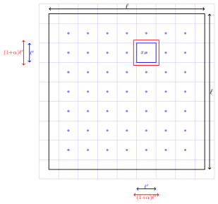
Figure 1. The square $Q_{\ell}$ decomposed into the small squares $\widetilde{Q}_{\ell^{\prime},i}$. Note the representation of the square $\widetilde{Q}_{\ell^{\prime},i}$ with center $x_{i}$ and the slightly larger square $Q_{\ell^{\prime},i}$.

The number $N$ satisfies

$$\left|N-\frac{\ell^{2}}{\ell^{\prime 2}}\right|\leq C\frac{\ell}{(\ell^{\prime})^{2}}\,.$$ (4.13)

Consider a partition of unity $(g_{i})$ satisfying in $Q_{\ell}$

$$\sum_{i}g_{i}=1\,,\quad\sum_{i}|\nabla g_{i}|^{2}\leq C(\ell^{\prime})^{-2}\alpha^{-2}\,,\quad{\rm supp}~{}g_{i}\subset Q_{\ell^{\prime},i}\,.$$

We have,

$$0\geq E_{\rm Ab}[\kappa-H]^{2}+o([\kappa-H]^{2}) \geq\mathcal{E}_{0}(\chi_{\ell}\psi,\mathbf{A}_{0};Q_{\ell})$$

$$\geq\sum_{i}\mathcal{E}_{0}(g_{i}\chi_{\ell}\psi,\mathbf{A}_{0};Q_{\ell^{\prime},i})-\ell^{2}[\kappa-H]^{2}o(1)\,.$$

Let $N_{+}={\rm Card},\mathcal{J}_{+}$ and $N_{-}={\rm Card}\,\mathcal{J}_{-}$, where

$$\mathcal{J}_{+}=\{i~{}:~{}q(g_{i}\chi_{\ell}\psi,\mathbf{A}_{0};Q_{\ell^{\prime},i})>0\}\,,\quad\mathcal{J}_{-}=\{i~{}:~{}q(g_{i}\chi_{\ell}\psi,\mathbf{A}_{0};Q_{\ell^{\prime},i})\leq 0\}\,,$$

and

$$q(g_{i}\chi_{\ell}\psi,\mathbf{A}_{0};Q_{\ell^{\prime},i})=\int_{Q_{\ell^{\prime},i}}\Big{(}|(\nabla-i\kappa H\mathbf{A}_{0})h_{i}v|^{2}-\kappa^{2}|h_{i}v|^{2}\Big{)}\,dx\,.$$

We have

$$\left|N_{-}-\frac{\ell^{2}\sqrt{\kappa H}}{\ell^{\prime 2}}\right|\leq\frac{\ell^{2}\sqrt{\kappa H}}{\ell^{\prime 2}}\,o(1)\,,\quad and\quad N_{+}=N_{-}o(1)\,.$$

Let $x_{i}$ denote the center of the square $Q_{\ell^{\prime},i}$, $R^{\prime}=\ell\sqrt{\kappa H}$ and $K_{R^{\prime}}=(-R^{\prime}/2,R^{\prime}/2)^{2}$. We introduce the two functions

$$h_{i}(x)=g\Big{(}x_{j}+\frac{x}{\sqrt{\kappa H}}\Big{)}\quad{\rm and}\quad v(x)=\left(\chi_{\ell}\psi\right)\Big{(}x_{i}+\frac{x}{\sqrt{\kappa H}}\Big{)}\,,\quad\big{(}\,x\in K_{R}^{\prime}\,\big{)}$$

As in the proof of Theorem 4.5, for all $i\in\mathcal{J}_{-}$, we have

$$\mathcal{E}_{0}(g_{i}\chi_{\ell}\psi,\mathbf{A}_{0};Q_{\ell^{\prime},i}) \geq\int_{K_{R}^{\prime}}\Big{(}\left(1-\frac{\kappa}{H}\right)|\Pi_{1}(h_{i}v)|^{2}+\frac{\kappa}{2H}|h_{i}v|^{4}\Big{)}\,dx$$

$$\geq\left[1-\frac{\kappa}{H}\right]_{+}^{2}\bigg{(}\left(1+2\left(\sigma+1-\frac{\kappa}{H}\right)\right)c(R^{\prime})-C\sigma^{-3}\left(1-\frac{H}{\kappa}\right)^{2}(R^{\prime})^{4}\bigg{)}\,,$$

and $\|h_{i}v-\Pi_{1}(h_{i}v)\|_{L^{2}(K_{R^{\prime}})}\ll\|h_{i}v\|_{L^{2}(K_{R^{\prime}})}$ , for all $\sigma\in(0,1/2)$. Note that our choice of $R^{\prime}$ allows us to choose $\sigma\ll 1$ such that $\sigma^{-3}\left(1-\frac{H}{\kappa}\right)^{2}(R^{\prime})^{4}\ll(R^{\prime})^{2}$. Thus, we get, for all $i\in\mathcal{J}_{-}$,

$$\mathcal{E}_{0}(g_{i}\chi_{\ell}\psi,\mathbf{A}_{0};Q_{\ell^{\prime},i}) \geq\int_{K_{R^{\prime}}}\Big{(}\left(1-\frac{\kappa}{H}\right)|\Pi_{1}(h_{i}v)|^{2}+\frac{\kappa}{2H}|h_{i}v|^{4}\Big{)}\,dx$$

$$\geq\left[1-\frac{\kappa}{H}\right]_{+}^{2}\bigg{(}c(R^{\prime})+o\big{(}(R^{\prime})^{2}\big{)}\bigg{)}\,.$$

We replace $\|\Pi(h_{i}v)\|_{2}$ by $\|h_{i}v\|_{2}$ and sum over $i\in\mathcal{J}_{-}$ to get,

$$\sum_{i\in\mathcal{J}_{-}}\int_{K_{R^{\prime}}}\Big{(}\left(1-\frac{\kappa}{H}\right)|h_{i}v|^{2}+\frac{\kappa}{2H}|h_{i}v|^{4}\Big{)}\,dx\\ \geq N_{-}\left[1-\frac{\kappa}{H}\right]_{+}^{2}\bigg{(}c(R^{\prime})+o\big{(}(R^{\prime})^{2}\big{)}\bigg{)}\,.$$

Since $h_{i}^{2}\geq h_{i}^{4}$, $c(R^{\prime})=(R^{\prime})^{2}E_{\rm Ab}+o((R^{\prime})^{2})$, $N_{-}=N+o(N)$ and $N$ satisfies (4.13), we get

$$\sum_{i\in\mathcal{J}_{-}}\int_{K_{R^{\prime}}}\Big{(}\left(1-\frac{\kappa}{H}\right)|h_{i}v|^{2}+\frac{\kappa}{2H}h_{i}^{2}|v|^{4}\Big{)}\,dx\\ \geq\ell^{2}\kappa H\sqrt{\kappa H}\left[1-\frac{\kappa}{H}\right]_{+}^{2}E_{\rm Ab}\bigg{(}1+o(1)\bigg{)}\,.$$

Using the bound $|v|\leq C(1-\frac{H}{\kappa})^{1/2}$ and that the number $N_{+}$ of indices in $\mathcal{J}_{+}$ is equal to $o(N)$, we get that the sum over $i\in\mathcal{J}$ satisfies,

$$\sum_{i\in\mathcal{J}}\int_{K_{R^{\prime}}}\Big{(}\left(1-\frac{\kappa}{H}\right)|h_{i}v|^{2}+\frac{\kappa}{2H}h_{i}^{2}|v|^{4}\Big{)}\,dx\\ \geq\ell^{2}\kappa H\sqrt{\kappa H}\left[1-\frac{\kappa}{H}\right]_{+}^{2}E_{\rm Ab}\bigg{(}1+o(1)\bigg{)}\,.$$

Now, noting that $\sum_{i\in\mathcal{J}}h_{i}^{2}=1$ and performing a change of variable, we get

$$\int_{Q_{\ell}}\Big{(}\left(1-\frac{\kappa}{H}\right)|\chi_{\ell}\psi|^{2}+\frac{\kappa}{2H}|\chi_{\ell}\psi|^{4}\Big{)}\,dx\\ \geq\ell^{2}\kappa H\sqrt{\kappa H}\left[1-\frac{\kappa}{H}\right]_{+}^{2}E_{\rm Ab}\bigg{(}1+o(1)\bigg{)}\,,$$

Using the asymptotics for $\|\chi_{\ell}\psi\|_{4}$ and a change of variables yields the following upper bound

$$\frac{1}{|Q_{\ell}|}\int_{Q_{\ell}}|\chi_{\ell}\psi|^{2}\,dx\leq-2E_{\rm Ab}\left[1-\frac{H}{\kappa}\right]+o\left(\left[1-\frac{H}{\kappa}\right]\right)\,.$$ (4.14)

We collect (4.12) and (4.14), then we use the assumption on the support of the function $\chi_{\ell}$, the bound (2.4) and the choice of $\ell$ to get,

$$\int_{Q_{\ell}}|\psi|^{2}\,dx=\int_{Q_{\ell}}|\chi_{\ell}\psi|^{2}\,dx+\mathcal{O}\left(\frac{\ell}{\sqrt{\kappa H}}\left[1-\frac{H}{\kappa}\right]\right)=E_{\rm Ab}\ell^{2}\left[1-\frac{H}{\kappa}\right]+o\left(\ell^{2}\left[1-\frac{H}{\kappa}\right]\right)\,.$$

This finishes the proof of Theorem 1.1. ∎

References

[1] A.A. Abrikosov. On the magnetic properties of
suerconductors of the second group. Soviet Phys. J.E.T.P.5 (1957), 1175-1204.
[2] A. Aftalion, X. B. Blanc, F. Nier. Lowest Landau level
functionals and Bargmann spaces for Bose-Einstein condensates. J. Funct. Anal.241 (2006), 661-702.
[3] A. Aftalion. S.
Serfaty. Lowest Landau level approach in superconductivity for the
Abrikosov lattice close to . Selecta Math. (N.S.)13 (2007), 183-202.
[4] Y. Almog. Abrikosov lattices in finite domains. Commun. Math. Phys.262 (2006), 677-702.
[5] Y. Almog, B. Helffer. The distribution of surface superconductivity along the boundary: on a conjecture of X.B.
Pan. SIAM J. Math. Anal.38 (2007), 1715–1732.
[6] M. Correggi, N. Rougerie. On the Ginzburg-Landau
functional in the surface superconductivity regime. Preprint, arXiv:1309.2268 (2013).
[7] S. Fournais, B. Helffer. Spectral Methods in
surface superconductivity. Progress in Nonlinear Differential
Equations and Their Applications. 77 Birkhäuser (2010).
[8] S. Fournais, B. Helffer. Bulk superconductivity in type
II superconductors near the second critical field. J. Europ. Math. Soc. (JEMS)12 (2008), 461-470.
[9] S. Fournais, B. Helffer. Optimal uniform elliptic estimates
for the Ginzburg-Landau system. Adventures in Mathematical Physics.
Contemp. Math.447 (2007), 83-102.
[10] S. Fournais, A. Kachmar. The ground state energy
of the three dimensional Ginzburg-Landau functional. Part I. Bulk
regime. Communications in Partial Differential Equations.38 (2013), 339-383.
[11] S. Fournais, A. Kachmar. Nucleation of bulk superconductivity close to critical magnetic field.
Advances in Mathematics226 (2011), 1213-1258.
[12] B. Helffer, X.-B. Pan. Upper critical field and location
of surface nucleation of superconductivity. Ann. Inst. H. Poincaré Anal. Non. Linéaire20
(2003), 145-181.
[13] K. Lu, X.B. Pan. Estimates of the upper critical
field for the Ginzburg-Landau equations of superconductivity. Physica D127 (1999), 73-104.
[14]
X.B. Pan. Surface superconductivity in applied magnetic fields above
. Commun. Math. Phys.228 (2002), 228-370.
[15] E. Sandier, S. Serfaty. Vortices for the Magnetic
Ginzburg-Landau Model. Progress in Nonlinear Differential Equations
and their Applications. 70 Birkhäuser (2007).
[16] E. Sandier, S. Serfaty. The decrease of bulk
superconductivity close to the second critical field in the
Ginzburg-Landau model. SIAM. J. Math. Anal.34 (2003),
939-956.