Testing locality and noncontextuality with the lowest moments

Abstract

The quest for fundamental test of quantum mechanics is an ongoing effort. We here address the question of what are the lowest possible moments needed to prove quantum nonlocality and noncontextuality without any further assumption – in particular without the often assumed dichotomy. We first show that second order correlations can always be explained by a classical noncontextual local-hidden-variable theory. Similar third-order correlations also cannot violate classical inequalities in general, except for a special state-dependent noncontextuality. However, we show that fourth-order correlations can violate locality and state-independent noncontextuality. Finally we obtain a fourth-order continuous-variable Bell inequality for position and momentum, which can be violated and might be useful in Bell tests closing all loopholes simultaneously.

I Introduction

Certain quantum correlations cannot be reproduced by any classical local-hidden-variable (LHV) theory, as they violate e.g. the Bell inequalities for correlations of results of measurements by separate observersbell . The Bell test must be performed under the following conditions: (i) dichotomy of the measurement outcomes or at least some restricted set of outcomes in some generalizations cglmp , (ii) freedom of choice of the measured observables will , and (iii) a shorter time of the choice and measurement of the observable than the communication time between the observers. Despite considerable experimental effort bellex , the violation has not yet been confirmed conclusively, due to several loopholes loop . The loopholes reflect the fact that the experiments have not fully satisfied all the conditions (i-iii) simultaneously. In fact, the Bell test is stronger than the entanglement criterion, viz. the nonseparability of states ent . The latter assumes already a quantum mechanical framework (e.g. an appropriate Hilbert space), while the former is formulated classically. The loophole-free violation of a Bell inequality – not just the existence of entanglement – is also necessary to prove the absolute security of quantum cryptography gis06 .

Nonclassical behavior of quantum correlations can appear also as a violation of noncontextuality. Noncontextuality means that the outcomes of experiments do not depend on the detectors’ settings so that there is a common underlying probability for the results of all possible settings while the accessible correlations correspond to commuting sets of observables. The Kochen-Specker theorem ingeniously shows that noncontextuality contradicts quantum mechanics kst , Noncontextuality is testable in realistic setups kst2 . In contrast to noncontextuality, Bell-type tests of nonlocality without further assumptions must exclude also contextual LHV models as correlations of outcomes for different settings are not simultaneously experimentally accessible for a single observer, even if they accidentally commute. Moreover, noncontextuality may be violated for an arbitrary localized state (state-independent noncontextuality stin ) while Bell-type tests make sense only for nonlocally entangled states. If a Bell-type inequality is violated then state-dependent noncontextuality is violated, too, but not vice-versa.

As the Bell and noncontextual inequalities are often restricted to dichotomic outcomes, e.g. $A=\pm 1$, generalizations have been investigated, including the many-outcome case cglmp . Recently, Cavalcanti, Foster, Reid and Drummond (CFRD) cfrd proposed a way to relax the constraint of dichotomy, allowing any unconstrained real value. CFRD constructed a particularly simple class of inequalities holding classically, while seemingly vulnerable by quantum mechanics. The inequalities involve $n$th moments $\langle A^{n-l-m}B^{l}C^{m}\rangle$ of observables $A$, $B$, $C$, and nonnegative integers $l,m$ and $n-l-m$, where in general the higher $n$ is, the greater the chances to violate the corresponding CFRD inequality. On a practical level, measuring higher moments or making binning is not a problem if the statistics consists of isolated peaks. However, in many experiments, especially in condensed matter three , the interesting information is masked by large classical noise. This noise then dominates the signal and makes the binning unable to retrieve the underlying quantum statistics, which is accessible only by measuring moments and subsequent deconvolution.

In this paper we ask which are the lowest possible moments to show nonclassicality and systematically investigate whether second-, third- or fourth-order correlations are sufficient to exclude LHV theories. We first show that second-order inequalities cannot be violated at all because of the so-called weak positivity bb11 – a simple classical construction of a probability reproducing all second-order correlations. Note that the standard Bell inequalities bell require experimental verification of the dichotomy $A^{2}=1$, which means e. g. showing that $\langle(A^{2}-1)^{2}\rangle=0$ by measuring the corresponding fourth-order correlator or applying binning (in which case the correlator is obviously zero). Hence, operationally a standard Bell test is of at least fourth order – not second, as it may appear from the Bell inequalities bell alone. We emphasize that binning is useless, if the signal is masked by classical noise. The proposed Bell-type tests in condensed matter based on second order correlations entsol ; entrev ; heiblum require an additional assumption of a dichotomous interpretation of the measurement results, which is in general experimentally unverified and does not allow entanglement to be identified unambiguously. Next we will show, that Bell-type tests for third moments with standard, projective measurements are not possible. Nevertheless, third moments can violate noncontextuality but only for a positive semidefinite correlation matrix and special states. Our main result is to show that generally fourth-order correlators are sufficient to violate state-independent noncontextuality and a Bell-type inequality which can be violated by correlation of position and momentum in a special entangled state. State-independent noncontextuality can be violated by a fourth-moment generalization of the Mermin-Peres square merper . Our results for the gradual possibilities of excluding LHV models under different conditions are summarized in Table 1.

Comparing to the previous research, note that the CFRD inequalities are the only known Bell-type inequalities scalable with $A\to\lambda A$, $B\to\mu B$ and so on for more observers. Unfortunately, the original example for a violation involved 20th-order correlators and 10 observers cfrd , but was later reduced to 6th order and 3 observers salles ; qhe for Greenberger-Horne-Zeilinger states ghz . On the other hand, the CFRD inequality with 4th moments cannot be violated at all, which has been shown for spins pro1 , quadratures pro2 , generalized to 8 settings and proved for separable states schvo , and finally proved for all states salles (we show an alternative proof in Appendix E).

The paper is organized as follows. We start with a general description of tests of contextuality and locality. Then we show that second moments are insufficient to violate locality and noncontextuality. Next, we show that third moments are enough only to show state-dependent contextuality. In the last part we discuss fourth moments, which allow violation of state-independent noncontextuality and locality. The violation of locality is possible with moments of positions/momenta (quadratures).

Noncontextuality	Yes	Yes	No
State independent	No	Yes	No
Maximal moments	LHV excluded?
2nd	No	No	No
3rd	Yes	No	No
4th	Yes	Yes	Yes

Table 1: Summary of the feasibility of moment-based tests of LHV theories depending on the conditions: a) contextuality or noncontextuality and b) special or arbitrary input state. The entries answer the questions: Are correlations with moments up to the given order not explicable by a joint positive probability?

II Test of local-hidden-variable models

Let us adopt the Bell framework, depicted in Fig. 1. Suppose Alice, Bob, Charlie, etc. are separate observers that can perform measurements on a possibly entangled state, which is described by an initial density matrix $\hat{\rho}$. Every observer $X=A,B,C,\dots$ is free to prepare one of several settings of their own detector ($\alpha=1,2,\dots$). For each setting, one can measure multiple real-valued observables (numbered $i=1,2,3,\dots$) so that the measurement of $\hat{X}_{\alpha i}$ gives a real number $X_{\alpha i}$ The projection postulate gives the quantum prediction for correlations, $\langle O_{1}\cdots O_{n}\rangle=\mathrm{Tr}\hat{\rho}\hat{O}_{1}\cdots\hat{O}_{n}$ for commuting observables $\hat{O}_{k}$. The observables measured by different observers and by one observer $\hat{X}_{\alpha i}$ for a given setting have to commute, viz. $[\hat{X}_{\alpha i},\hat{Y}_{\beta j}]=[\hat{X}_{\alpha i},\hat{X}_{\alpha j}]=0$. The observables for one observer but different settings, $\hat{X}_{\alpha i}$ and $\hat{X}_{\beta j}$ for $\alpha\neq\beta$, may be noncommuting but may also accidentally commute or even be equal. A LHV model assumes the existence of a joint positive-definite probability distribution of all possible outcomes $\rho(\{X_{\alpha i}\})$ that reproduces quantum correlations for a given setting. If the accidental equality between observables for different settings, $\hat{X}_{\alpha i}=\hat{X}_{\beta j}$, imposes the constraint ${X}_{\alpha i}\equiv{X}_{\beta j}$ in $\rho$, the LHV model is called noncontextual. A single observer suffices to test such LHV as noncontextuality is anyway an experimentally unverifiable assumption – the observer cannot measure simultaneously at two different settings. In contrast to noncontextuality, the locality test must allow contextuality: that even if $\hat{X}_{\alpha i}=\hat{X}_{\beta j}$ ($\alpha\neq\beta$) then ${X}_{\alpha i}\neq{X}_{\beta j}$ is still possible. The choices of the settings and measurements are required to be fast enough to prevent any communication between observers. Then $\rho$ cannot be altered by the choice of the observable. Noncontextual and local LHVs can be ruled out by tests with discrete outcomes bell ; kst . In moment-based tests only a finite number of cross correlations are compared with LHV. Our aim is to find the lowest moments showing nonclassical behavior of quantum correlations.

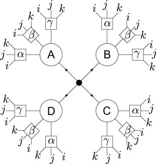
Figure 1: The general test of local realism. Here we have four observers, Alice, Bob, Charlie and David. Everybody is free to choose between three different settings, $\alpha$, $\beta$ and $\gamma$ and finally they can measure three real, continuous outcomes, e.g. $A_{\alpha i}$. The picture can be generalized to arbitrary numbers of observers, settings and outcomes.

III Weak positivity

For a moment all observables, commuting or not, will be denoted by $\hat{X}_{i}$. Let us recall the simple proof that first- and second-order correlations functions can be always reproduced classically bb11 . To see this, consider a real symmetric correlation matrix

$$\mathcal{C}_{ij}=\langle X_{i}X_{j}\rangle=\mathrm{Tr}\hat{\rho}\{\hat{X}_{i},\hat{X}_{j}\}/2$$ (1)

with $\{\hat{X},\hat{Y}\}=\hat{X}\hat{Y}+\hat{Y}\hat{X}$ for arbitrary observables $\hat{X}_{i}$ and density matrix $\hat{\rho}$. Such a relation is consistent with simultaneously measurable correlations. More generally, it holds even in the noncontextual case, when observables from different settings commute. Only these elements of the matrix $\mathcal{C}$ are measurable, for the rest (1) is only definition. Our construction includes all possible first-order averages $\langle X_{i}\rangle$ by setting one observable to identity or subtracting averages ($X_{i}\to X_{i}-\langle X_{i}\rangle$). Since $\mathrm{Tr}\hat{\rho}\hat{W}^{2}\geq 0$ for $\hat{W}=\sum_{i}\lambda_{i}\hat{X}_{i}$ with arbitrary real $\lambda_{i}$, we find that the correlation matrix $\mathcal{C}$ is positive definite. Therefore every correlation can be simulated by a classical Gaussian distribution $\varrho\propto\exp(-\sum_{ij}{{\mathcal{C}}^{-1}}_{ij}X_{i}X_{j}/2)$, with $\mathcal{C}^{-1}$ being the matrix inverse of $\mathcal{C}$. This is a LHV model reproducing all measurable correlations. We recall that we do not assume dichotomy $X=\pm 1$, which is equivalent to $\langle(X^{2}-1)^{2}\rangle=0$ and requires $\langle X^{4}\rangle$. For simplicity, from now on we shall fix $\langle X_{i}\rangle=0$, redefining all quantities $X_{i}\to X_{i}-\langle X_{i}\rangle$.

It is interesting to note that Tsirelson’s bound cir can be seen as consequence of weak positivity. Taking observables $A_{1}$, ${A}_{2}$, ${B}_{1}$, and ${B}_{2}$, we have

$$\langle(\sqrt{2}A_{1}-B_{1}-B_{2})^{2}\rangle+\langle(\sqrt{2}A_{2}-B_{1}+B_{2})^{2}\rangle\geq 0$$ (2)

for the Gaussian distribution with the correlation matrix (1). It is equivalent to

$$\langle A_{1}B_{1}\rangle+\langle A_{1}B_{2}\rangle+\langle A_{2}B_{1}\rangle-\langle A_{2}B_{2}\rangle$$

$$\leq(\langle A^{2}_{1}\rangle+\langle A^{2}_{2}\rangle+\langle B^{2}_{1}\rangle+\langle B^{2}_{2}\rangle)/\sqrt{2}.$$ (3)

For $A,B=\pm 1$, the right hand side gives Tsirelson’s bound $2\sqrt{2}$ which is at the same time the maximal quantum value of the left-hand side. On the other hand, the upper classical bound in this case is $2$ bell , but it requires assuming dichotomy or equivalently knowledge of higher moments.

IV Third Moments

Having learned that second moments do not show nonclassicality at all, we turn to third moments. If the matrix $\mathcal{C}$ is strictly positive definite, all third order correlations can be explained by a positive probability as well (the proof in Appendix A). The problematic case is a semipositive-definite $\mathcal{C}$, with at least one $0$ eigenvalue. One cannot violate noncontextuality with an arbitrary state and third-order correlations. To see this, let us take the completely random state $\hat{\rho}\propto\hat{1}$ and suppose that the correlation matrix (1) has a zero eigenvalue for $\hat{W}=\sum_{k}\lambda_{k}\hat{X}_{k}$. Then $\langle W^{2}\rangle=0$ and $\mathrm{Tr}\hat{W}^{2}=0$, which gives $\hat{W}=0$. We can simply eliminate one of observables by the substitution $\hat{X}_{m}=-\sum_{k\neq m}\lambda_{k}\hat{X}_{k}/\lambda_{m}$ using the symmetrized order of the operators when noncommuting products appear. Now the remaining correlations matrix $C_{ij}$ with $i,j\neq m$ is positive definite and the proof in Appendix A holds. If the correlation matrix has more zero eigenvalues, we repeat the reasoning, until only nonzero eigenvalues remain. Furthermore, third-order correlations alone cannot show noncontextuality in a state-dependent way for up to 4 observables, nor in any two-dimensional Hilbert space, nor they can violate local realism (proofs in Appendices B and C). There exists, however, an example of violation of state-dependent noncontextuality with five observables in three-dimensional space (Appendix D).

Instead, here we show a simple example violating state-dependent noncontextuality, based on the Greenberger-Horne-Zeilinger (GHZ) idea ghz . We consider a three qubit Hilbert space with the 8 basis states are denoted $|\epsilon_{1}\;\epsilon_{2}\;\epsilon_{3}\rangle$ with $\epsilon_{\alpha}=\pm$. We have three sets of Pauli matrices $\hat{\sigma}^{(\alpha)}_{j}$, with $\hat{\sigma}_{1}=|-\rangle\langle+|+|+\rangle\langle-|$ and $\hat{\sigma}_{2}=i|-\rangle\langle+|-i|+\rangle\langle-|$, acting only in the respective Hilbert space of qubit $\alpha$. Now let us take the six observables, $\hat{A}_{\alpha}=\hat{\sigma}^{(\alpha)}_{1}$ , $\hat{B}_{\alpha}=\hat{C}\hat{\sigma}^{(\alpha)}_{2}$ for $\alpha=1,2,3$ and $\hat{C}=\hat{\sigma}^{(1)}_{2}\hat{\sigma}^{(2)}_{2}\hat{\sigma}^{(3)}_{2}$. All $\hat{A}$’s commute with each other, similarly all $\hat{B}$’s commute, and $\hat{A}_{\alpha}$ commutes with $\hat{B}_{\alpha}$. We take $\hat{\rho}=|\mathrm{GHZ}\rangle\langle\mathrm{GHZ}|$ for the GHZ state

$$\sqrt{2}|\mathrm{GHZ}\rangle=|++\>+\rangle+|--\>-\rangle.$$ (4)

Assuming noncontextuality, we have

$$\langle(A_{\alpha}+B_{\alpha})^{2}\rangle=\mathrm{Tr}\hat{\rho}(\hat{A}_{\alpha}+\hat{B}_{\alpha})^{2}=0,$$ (5)

which implies $A_{\alpha}=-B_{\alpha}$, so classically $\langle A_{1}A_{2}A_{3}\rangle=-\langle B_{1}B_{2}B_{3}\rangle$. However,

$$\langle A_{1}A_{2}A_{3}\rangle=\mathrm{Tr}\hat{\rho}\hat{A}_{1}\hat{A}_{2}\hat{A}_{3}=1,$$

$$\langle B_{1}B_{2}B_{3}\rangle=\mathrm{Tr}\hat{\rho}\hat{B}_{1}\hat{B}_{2}\hat{B}_{3}=1,$$ (6)

in contradiction with the earlier statement and excluding noncontextual LHVs. Hence, we have seen that the third order correlations may violate noncontextuality for specific states. It should not be surprising that the test is based on violating an equality, instead of an inequality, because third moments can have arbitrary signs.

V Fourth-order correlations: noncontextuality

To find a test of noncontextuality we now consider fourth moments. Mermin and Peres merper have shown a beautiful example of state-independent violation of noncontextuality using observables on the tensor product of two two-dimensional Hilbert spaces $\mathcal{H}_{A}\otimes\mathcal{H}_{B}$ arranged in a square

$$\begin{array}[]{|c|c|c|c|}\hline\cr\hat{M}_{ij}&j=1&j=2&j=3\\ \hline\cr i=1&\hat{\sigma}^{A}_{1}&\hat{\sigma}^{A}_{1}\hat{\sigma}^{B}_{1}&\hat{\sigma}^{B}_{1}\\ \hline\cr i=2&-\hat{\sigma}^{A}_{1}\hat{\sigma}^{B}_{3}&\hat{\sigma}^{A}_{2}\hat{\sigma}^{B}_{2}&-\hat{\sigma}^{A}_{3}\hat{\sigma}^{B}_{1}\\ \hline\cr i=3&\hat{\sigma}^{B}_{3}&\hat{\sigma}^{A}_{3}\hat{\sigma}^{B}_{3}&\hat{\sigma}^{A}_{3}\\ \hline\cr\end{array}$$ (7)

where the Pauli observables $\hat{\sigma}_{i}$ are in each Hilbert space ($\{\hat{\sigma}_{i},\hat{\sigma}_{j}\}=2\delta_{ij}\hat{1}$). Observables in each row and each column commute. We denote products in each column $\hat{C}_{i}=\hat{M}_{1i}\hat{M}_{2i}\hat{M}_{3i}$ and row $\hat{R}_{i}=\hat{M}_{i1}\hat{M}_{i2}\hat{M}_{i3}$. We get $\hat{C}_{i}=-\hat{1}$ and $\hat{R}_{i}=\hat{1}$. If $\hat{M}_{ij}$ are replaced by classical variable $M_{ij}$ then $C_{1}C_{2}C_{3}=R_{1}R_{2}R_{3}$ in contradiction with the quantum result.

Now we assume that the $M$ are not spin-$1/2$, but arbitrary operators, which can grouped into a Mermin-Peres square fulfilling the corresponding commutation relations, $[\hat{M}_{ij},\hat{M}_{ik}]=[\hat{M}_{ij},\hat{M}_{kj}]=0$ (operators in the same column or row commute). We will show that in this example the dichotomy test can be avoided by fourth-order correlations, without other assumptions on values $M_{ij}$. To see this, note that $S\equiv\sum_{i}(C_{i}-R_{i})=\det N,$ where $N_{ij}=M_{i+j,i-j}$ (counting modulo 3). Now, we note that $(\det N)^{2}=\det(N^{T}N)$ and the eigenvalues $\lambda_{i}$ of $N^{T}N$ are real and positive. Using the Cauchy inequality we find that $\det(N^{T}N)=\lambda_{1}\lambda_{2}\lambda_{3}\leq(\lambda_{1}+\lambda_{2}+\lambda_{3})^{3}/27=(\mathrm{Tr}N^{T}N)^{3}/27$. We get then

$$3\sqrt{3}|S|\leq\left(\sum\nolimits_{ij}M_{ij}^{2}\right)^{3/2}\leq 3\sum\nolimits_{ij}|M_{ij}|^{3}$$ (8)

where we used the Hölder inequality in the last step. Now, we take the average of the above equation, use $|\langle S\rangle|\leq\langle|S|\rangle$ and apply the Cauchy-Bunyakovsky-Schwarz inequality $\langle|xy|\rangle\leq(\langle x^{2}\rangle\langle y^{2}\rangle)^{1/2}$ to $x=M_{ij}$ and $y=M_{ij}^{2}$. We obtain finally an inequality obeyed by all noncontextual theories

$$|\langle S\rangle|\leq\sum\nolimits_{ij}\left[\langle M_{ij}^{2}\rangle\langle M_{ij}^{4}\rangle/3\right]^{1/2}.$$ (9)

The inequality involves maximally fourth-order correlations and every correlation is measurable (corresponds to commuting observables). One can check that if $M_{ij}$ correspond to (7) then the left-hand side of (9) is $6$ while the right-hand side of (9) is $3\sqrt{3}$, giving a contradiction. Hence, a violation of (9) is possible, but it remains to be shown that systems with naturally continuous variables violate are contextual by violating Eq. (9) or other fourth-moment-based inequalities.

VI Fourth-order correlations: nonlocality

A simple fourth-moment-based inequality testing local realism has been considered by CFRD cfrd

$$\langle A_{1}B_{1}-A_{2}B_{2}\rangle^{2}+\langle A_{1}B_{2}+A_{2}B_{1}\rangle^{2}\leq\langle(A_{1}^{2}+A_{2}^{2})(B_{1}^{2}+B_{2}^{2})\rangle.$$ (10)

Note that all averages involve only simultaneously measurable quantities. This constitutes an inequality, which holds classically, involves only 4th-order averages and is scalable with respect to $A$ and $B$. Unfortunately, (10) and its generalizations schvo are not violated at all in quantum mechanics as shown in salles . We present an alternative proof in Appendix E.

Unfortunately a violable two-party fourth-order inequality is much more complicated bb11 . A different, but quadripartite inequality can be obtained by a slight modification of CFRD inequalities cfrd . It reads

$$|\langle ABCD\rangle|^{2}\leq\langle|AB|^{2}\rangle\langle|CD|^{2}\rangle$$ (11)

where $A=A_{1}+iA_{2}$ etc., so that both sides, when expanded, contain only simultaneously measurable correlations (because $|\langle ABCD\rangle|^{2}=\langle\mathrm{Re}ABCD\rangle^{2}+\langle\mathrm{Im}ABCD\rangle^{2}$ is free from products $\langle A_{1}A_{2}\cdots\rangle$ and $|A|^{2}=A_{1}^{2}+A_{2}^{2}$ on the right-hand side) It follows from the generalized triangle inequality $|\langle Z\rangle|\leq\langle|Z|\rangle$ for $Z=ABCD$ and the Cauchy-Bunyakovsky-Schwarz inequality $\langle XY\rangle^{2}\leq\langle X^{2}\rangle\langle Y^{2}\rangle$ for $X=|AB|$ and $Y=|CD|$. See more details in Appendix F.

Interestingly, the inequality (11) can be violated by correlations of positions and momenta, Let us take standard harmonic oscillator operators $\sqrt{2}\hat{A}=\hat{X}_{A}+i\hat{P}_{A}$ with $[\hat{X}_{A},\hat{P}_{A}]=i$ ($\hbar=1$) so $A_{1}\to\hat{X}_{A}/\sqrt{2}$, $A_{2}\to\hat{P}_{A}/\sqrt{2}$, and $[\hat{A},\hat{A}^{\dagger}]=1$ and analogously for $B$, $C$, and $D$. In the Fock basis $\hat{A}|n\rangle_{A}=\sqrt{n}|n-1\rangle_{A}$ etc. Now take a specific entangled state in the product space of $A$,$B$,$C$, and $D$, $|\psi\rangle=\sum_{n\geq 0}^{N}z_{n}|nnnn\rangle$ with real $z_{n}$ (for simplicity) and check if (11) holds also quantum mechanically. We find that $\langle\psi|\hat{A}\hat{B}\hat{C}\hat{D}|\psi\rangle=\sum_{n}n^{2}z_{n}z_{n-1}$ while $\langle\psi|(\hat{A}^{\dagger}\hat{A}+\hat{A}\hat{A}^{\dagger})(\hat{B}^{\dagger}\hat{B}+\hat{B}\hat{B}^{\dagger})|\psi\rangle=\sum_{n}z_{n}^{2}(2n+1)^{2}$, and similarly for $C$ and $D$. Due to symmetry between the oscillators, the inequality (11) is equivalent to $\langle ABCD\rangle\leq\langle|AB|^{2}\rangle$, and the quantum mechanical prediction reads $\sum_{n=0}^{N}n^{2}z_{n}z_{n-1}\leq\sum_{n=0}^{N}z_{n}^{2}(n+1/2)^{2}$. This is equivalent to the positivity of the $(N+1)\times(N+1)$ matrix $M$ with entries $M_{nn}=(n+1/2)^{2}$ for $n=0,1,\dots,N$ and $M_{n,n+1}=M_{n+1,n}=-(n+1)^{2}/2$ for $n=0,1,\dots,N-1$, and $0$ otherwise. However, for $N\geq 10$ we get $\det{M}<0$ so it must have a negative eigenvalue. A numerical check for $N=10$ shows that e.g. the state with the $\{z_{n}\}=\{0.83,0.42,0.27,0.18,0.13,0.09,0.07,0.05,0.03,0.02,0.01\}$ violates (11). The generation of the highly entangled state violation (11) will be difficult but possible because techniques of generation of multipartite entangled optical states already exist pan .

VII Conclusions

We have proved that one cannot show nonclassicality by violating inequalities containing only up to third-order correlations, except state-dependent contextuality. Fourth order correlations are sufficient to violate locality and state-independent noncontextuality but the corresponding inequalities are quite complicated. A fourth order quadripartite Bell-type inequality (11) can be violated by 4th-order correlations of position and momentum or quadratures for special entangled states.

Appendix A. Positive definite correlations

Let us assume that the correlation matrix $\mathcal{C}$ from (1) is strictly positive definite, having all eigenvalues positive. We will prove that every third order correlation can explained also by a positive probability. We also shift all first order averages to zero, $X_{i}\to X_{i}-\langle X_{i}\rangle$. So far the distribution of $X$ was Gaussian and $X$ were continuous, but in this case all central third moments are zero. To allow for nonzero third moments we have to change the probability. The simplest (but not the only) way is to change the probability at particular values of $X$ to get a non-Gaussian distribution. We define additional labels $\{ijkq\}$, $i\neq j\neq k\neq i$ (in this case one for all possible permutations of $ijk$), $\{ijq\pm\}$, $i\neq j$, $\{ijq\pm\}\neq\{jiq\pm\}$ (here order matters), and $\{iq\}$ with an auxiliary parameter $q\in\{3,-1,-2\}$. The modified distribution reads

$$\varrho(X)=\varrho_{G}(X)+\lambda^{-3}\sum_{L}\prod_{j}\delta(X_{j}-W_{j}(L)),$$

$$\varrho_{G}(X)=\frac{1-c/\lambda^{3}}{(2\pi)^{n/2}(\det\mathcal{C})^{1/2}}e^{-\sum_{ij}\mathcal{C}^{-1}_{ij}X_{i}X_{j}/2},$$ (A.1)

where $\varrho_{G}$ is the ”old” Gaussian (renormalized) while the second part is the sum over delta peaks at particular points depending on the label $L$. Here $c$ is the number of all labels $L$ and $\lambda>0$ is some very large real parameter such that $c/\lambda^{3}<1$. The positions of the peaks are

$$W_{i,j,k}(\{ijkq\})=q\lambda\langle X_{i}X_{j}X_{k}\rangle^{1/3}/\sqrt[3]{18},$$ (A.2)

$$W_{i}(\{ijq\pm\})=\pm\sqrt{2}qQ_{ij}/\sqrt[3]{18},$$

$$W_{j}(\{ijq\pm\})=qQ_{ij}/\sqrt[3]{18},$$

$$Q_{ij}=\frac{\lambda}{\sqrt[3]{4}}\left[\langle X^{2}_{i}X_{j}\rangle-\sum_{k\neq ij}\langle X_{i}X_{j}X_{k}\rangle\right]^{1/3},$$

$$W_{i}(\{iq\})=\frac{q\lambda}{\sqrt[3]{18}}\left[\langle X^{3}_{i}\rangle-\sum_{j\neq i}\langle X^{2}_{j}X_{i}\rangle/2\right]^{1/3}$$

$$W_{l}(\{ijkq\})=W_{l}(\{ijq\pm\})=W_{l}(\{iq\})=0,\>l\neq ijk.$$

The cubic root is defined real for real negative arguments. Here $\langle X_{i}X_{j}X_{k}\rangle$ are the desired third moments (the argument holds even for noncommuting observables). Note that the special choice of $q$ results in unchanged averages $\langle X_{i}\rangle$ as $3-1-2=0$ but nonzero third order averages as $3^{3}-1^{3}-2^{3}=18$. The calculation of the third moments gives exactly the desired values. Unfortunately, it will modify the correlation matrix $\mathcal{C}$. However, the correction is $\sim 1/\lambda$. The modified correlation matrix is then arbitrarily close to ${\mathcal{C}}$ at $\lambda\to\infty$, so it must be positive definite and we can find the new Gaussian part in the form $\varrho_{G}\propto\exp(-\sum_{ij}{{\mathcal{C}}^{\prime-1}}_{ij}X_{i}X_{j}/2)$, where the matrix $\mathcal{C}^{\prime}$ gives the correct total second-order correlations.

The assignment (A.2) is certainly not unique, one could easily find a lot of different ones also reproducing correctly third order correlations. However, the bottom line is that the proof works only if $\mathcal{C}$ has positive signature. If some eigenvalues of $\mathcal{C}$ are $0$ (which occurs when a particular $X_{i}$ is in fact linearly dependent on the others) then ${\mathcal{C}}^{\prime}$ may have a negative eigenvalue for arbitrary $\lambda$ and we cannot find any Gaussian distribution, as shown in the example in Section IV.

Appendix B. Noncontextuality in simple cases

Let us examine state-dependent noncontextuality with up to 4 observables, $\hat{A}_{i}$, $i=1,2,3,4$ with the outcomes $A_{i}$ or $A,B,C,D$. We look for a positive probability $\varrho(\{A_{i}\})$ that reproduces correctly all first, second and third moments calculated by quantum rules. We have the freedom to set values of correlations of noncommuting products of observables because they are not measurable simultaneously. The construction of the probability depends on the commutation properties of the set $\{\hat{A}_{i}\}$ and is shown for various cases in Table 2. We denote $\rho(\{A_{i}\})=\mathrm{Tr}\hat{\rho}\prod_{i}\delta(A_{i}-\hat{A}_{i})$ for every subset of commuting $\hat{A}_{i}$.

Observables	$\varrho(A,B,C,D)$
$A$ $B$ $C$ $D$	$\rho(A)\rho(B)\rho(C)\rho(D)$
$A-B$ $C$ $D$	$\rho(A,B)\rho(C)\rho(D)$
$A$ $\>D$ $/\>\>\>\backslash\quad$ $B-C\quad$	$\rho(A,B,C)\rho(D)$
$A$ $D$ $B-C$	$\rho(A)\rho(B,C)\rho(D)$
$B-A-C$ $D$	$\rho(A,B)\rho(A,C)\rho(D)/\rho(A)$
$B-A-D$ $|$ $C$	$\rho(A,B)\rho(A,C)\rho(A,D)/\rho^{2}(A)$
$A-D$ $/\>\>\>\backslash\quad\quad$ $B-C\quad\quad$	$\rho(A,B,C)\rho(A,D)/\rho(A)$
$A-D$ $|\times|$ $B-C$	$\rho(A,B,C,D)$
$A-B-C-D$	$\rho(A,B)\rho(B,C)\rho(C,D)/\rho(B)\rho(C)$
$A-B$ $C-D$	$\rho(A,B)\rho(C,D)$
$A$ $/\>\>\>\backslash$ $B-C$ $\backslash\>\>\>/$ $D$	$\rho(A,B,C)\rho(B,C,D)/\rho(B,C)$
$A_{1}-B_{1}$ $|\quad\quad|$ $B_{2}-A_{2}$	Appendix C

Table 2: Construction of positive probabilities $\varrho$ for all cases of up to 4 observables. Here the link $-$ means the observables commute (not linked do not commute). Exceptions: $\varrho=0$ when the denominator is zero.

The only difficult case is with noncommuting pairs $(\hat{A}_{1},\hat{A}_{2})$ and $(\hat{B}_{1},\hat{B}_{2})$ but this is equivalent to the test of local realism. We will show in the general proof that this case can be always (if we do not use fourth moments) explained by a LHV model in Appendix C. Thus, we have shown that it is possible to define positive probability distributions $\varrho$ that reproduces all quantum first, second, and third moments of measurable (commuting) combinations of up to 4 observables.

In two-dimensional Hilbert space the situation is somewhat simpler and we can find a classical construction for an arbitrary number of observables (not limited to 4). Observables have the structure $\hat{A}=a_{0}\hat{1}+\vec{a}\cdot\hat{\vec{\sigma}}$, where $\hat{\vec{\sigma}}=(\hat{\sigma}_{1},\hat{\sigma}_{2},\hat{\sigma}_{3})$ with standard Pauli matrices $\hat{\sigma}_{j}$, satisfying $\{\hat{\sigma}_{j},\hat{\sigma}_{m}\}=2\delta_{jm}\hat{1}$. Observables $\hat{A}$ and $\hat{B}$ commute if and only if $\vec{a}\parallel\vec{b}$. We can group all observables (their number is arbitrary) parallel to the same direction, so that $\vec{a}_{\alpha}\parallel\vec{a}$, $\vec{b}_{\beta}\parallel\vec{b}$, $\vec{c}_{\gamma}\parallel\vec{c}$, $\dots$, where $\vec{a}\nparallel\vec{b},\vec{c},\dots$, $\vec{b}\nparallel\vec{c},\dots$, etc.. Then we construct a LHV model defined by $\varrho(\{A_{\alpha}\},\{B_{\beta}\},\{C_{\gamma}\},\dots)=\rho(\{A_{\alpha}\})\rho(\{B_{\beta}\})\rho(\{C_{\gamma}\})\cdots$, where $\rho(\{A_{\alpha}\})=\mathrm{Tr}\hat{\rho}\prod_{j}\delta(A_{\alpha}-\hat{A}_{\alpha})$ and similar for the other sets. This means that all (noncontextual) third moments for a two-level system are reproduced by a classical probability.

On the other hand we will see in Appendix D an example of the violation of state-dependent noncontextuality involving a three-dimensional Hilbert space and 5 observables.

Appendix C. Third moments – contextual LHV models

We will present a general proof that third order correlations can be explained by a LHV model, if contextuality is allowed and no assumption on higher order moments or dichotomy is made. As in Section II, we denote $\mathcal{C}_{X\alpha j,Y\beta k}=\langle X_{\alpha j}Y_{\beta k}\rangle$ for $X,Y=A,B,C,\dots$ and $\alpha,\beta,j,k=1,2,\dots$. For a valid LHV theory, $\mathcal{C}$ must be positive (semi)definite.

1 Assumptions

The proof is based on two facts:

• $\mathcal{C}_{X\alpha j,X\beta k}=\langle X_{\alpha j}X_{\beta k}\rangle$ is not measurable for $\alpha\neq\beta$ (even if accidentally $\hat{X}_{\alpha j}\hat{X}_{\beta k}=\hat{X}_{\beta k}\hat{X}_{\alpha j}$) because $\alpha$ and $\beta$ correspond to two different settings of the same observer which cannot be realized simultaneously. So it is a free parameter in a LHV model.

• We can always redefine every observable within one observer’s setting by a real linear transformation $\hat{X}_{\alpha m}\to\sum_{k}\lambda_{\alpha k}\hat{X}_{\alpha k}$ as long as the linear independence is preserved, because all such observables commute with each other.

The proof involves a kind of Gauss elimination on a set of linear equations algebra .

2 Problem of zero eigenvalues

The first choice for $\mathcal{C}$ will be (1), which is positive semidefinite. We shall see that this choice must be sometimes modified, without affecting the measurable correlations. Suppose that the correlation matrix $\mathcal{C}$ has $\mathcal{N}$ zero eigenvalues with linearly independent zero eigenvectors

$$W_{m}=\sum_{\alpha,k}^{X=A,B,...}\lambda^{m}_{X\alpha k}X_{\alpha k}\,,\,m=1..\mathcal{N}$$ (C.1)

with the property $\langle W_{m}^{2}\rangle=0$. This implies $\mathrm{Tr}\hat{\rho}\hat{W}_{m}^{2}=0$, which gives

$$W_{m}=\hat{W}_{m}\hat{\rho}=0,\>m=1..\mathcal{N}.$$ (C.2)

The above set of linear equations can be modified as in usual algebra, we can multiply equations by nonzero numbers and add up, as long as the linear independence holds. Vectors $W_{m}$ span the kernel of the correlation matrix. We shall prove that for a given observer $X$ the above set of equations can be written in the form

$$X_{\alpha k}+\sum_{\beta j}^{Y\neq X}\lambda^{X\alpha k}_{Y\beta j}Y_{\beta j}=0$$ (C.3)

where we sum over all observers different from $X$ and all their settings and observables plus equations not containing $X$. If this were not possible then we shall prove that we can reduce the kernel by at least one vector by modifying nonmeasurable correlations in the correlation matrix, keeping its positivity. By such successive reduction we will end up with (C.3). For the Bell case ($A$ and $B$, $\alpha=1,2$) (C.3) reduces either to trivial single vectors $A_{\alpha}-\lambda B_{\alpha}$ or a set

$$\left\{\begin{array}[]{ccc}A_{1}&=&\lambda_{11}B_{1}+\lambda_{12}B_{2}\\ A_{2}&=&\lambda_{21}B_{1}+\lambda_{22}B_{2}\end{array}\right.$$ (C.4)

with invertible matrix $\lambda$. The original correlation matrix (1) may lead us into troubles for some correlations (violation of noncontextuality), which are anyhow unobservable so we do not need to bother in contextual LHV models. Therefore, sometimes we have to modify it slightly to relax dangerous constraints. The resulting LHV correlation matrix can be different from (1) but only for nonmeasurable correlations. We make use of the fact that quantum mechanics does not permit to measure everything in one run of the experiment, leaving more freedom for contextual LHV models.

3 Reduction of zero eigenvectors

We shall prove that all zero eigenvectors can be eliminated except those in the form of (C.3). Without loss of generality let us take $X=A$. We write (C.2) in the form

$$\sum_{\alpha k}\lambda_{\alpha k}^{m}A_{\alpha k}+\displaystyle{\not}A=0,$$ (C.5)

where $\displaystyle{\not}A$ replaces all linear combinations of quantities measured by the other observers ($B$, $C$, $D$, …), e.g. $\displaystyle{\not}A$ can be $2B_{11}-3B_{11}+B_{21}-5C_{13}$. By linear eliminations and transformations within setting $1$, there exists a form of (C.5) consisting of

$$A_{1k}+\displaystyle{\not}1+\displaystyle{\not}A=0,\>k=1,2,\dots,$$ (C.6)

with $\displaystyle{\not}1$ not containing $A_{1j}$ terms, and other equations that do not contain $A_{1j}$ at all. Suppose that at least one of (C.6) contains an $A_{2j}$ term, so in general (C.6) has the form

$$A_{1k}+\sum_{m}\lambda_{km}A_{2m}+\displaystyle{\not}1\displaystyle{\not}2+\displaystyle{\not}A=0,\>k=1,2,\dots$$ (C.7)

with at least one $\lambda_{km}\neq 0$ and $\displaystyle{\not}1\displaystyle{\not}2$ denoting all terms not containing $A_{1j}$ and $A_{2j}$. By linear eliminations and transformations within settings $1$ and $2$ we arrive at

$$A_{1k}+A_{2k}+\displaystyle{\not}1\displaystyle{\not}2+\displaystyle{\not}A=0,\>k=1,2,\dots,l$$

$$A_{1k}+\displaystyle{\not}1\displaystyle{\not}2+\displaystyle{\not}A=0,\>k=l+1,l+2,\dots,$$ (C.8)

$$A_{2k}+\displaystyle{\not}1\displaystyle{\not}2+\displaystyle{\not}A=0,\>k=l+1,l+2,\dots,$$

and other equations that do not contain $A_{1j}$ nor $A_{2j}$ at all (if we have a single observable for each setting then we can omit the index $k$). If $l>0$ then we change $\langle A_{11}A_{21}\rangle\to\langle A_{11}A_{21}\rangle+\epsilon$ with $\epsilon>0$ in the correlation matrix $\mathcal{C}$ (or $\langle A_{1}A_{2}\rangle$ for single observables). Then $\langle W^{2}\rangle=2\epsilon>0$, where $W$ is the left hand side of the first line in (C.8) for $k=1$. Correlations involving other kernel vectors remain unaffected as none of them contains $A_{11}$ nor $A_{21}$. For sufficiently small, but positive $\epsilon$ the new correlation matrix $\mathcal{C}$ will be strictly positive for in the space spun by the old non-kernel vectors plus $W$. In this way we reduce by $1$ the dimension of the kernel. By repeating this reasoning we kick out of the kernel all vectors on the left hand side of the first line of (C.8). Once we are left with only two last lines of (C.8) we proceed by induction.

Let us assume that, at some stage with a fixed $\alpha$, the kernel equations have the form

$$A_{\xi k}+\sum_{m}\lambda^{\xi}_{km}A_{\alpha m}+\displaystyle{\not}1\cdots\displaystyle{\not}\alpha+\displaystyle{\not}A=0$$ (C.9)

for all $\xi<\alpha$ plus other equations not containing $A_{\xi}$ and $A_{\alpha m}$. Note that the set of possible $k$ can be different for different $\xi$. If all $\lambda=0$ then we can proceed to the next induction step, taking next setting. Otherwise, let us denote by $\Xi$ the set of all $\xi$ with $\lambda^{\xi}_{k1}\neq 0$ for some $k$ (we fix the other index to $1$ without loss of generality). By linear eliminations we find only one such $k$ for each $\xi\in\Xi$ so that $\lambda^{\xi}_{k1}=\delta_{k1}$. Now, we make a shift of the nonmeasurable correlations $\langle A_{\xi 1}A_{\alpha 1}\rangle\to\langle A_{\xi 1}A_{\alpha 1}\rangle+\epsilon$ and $\langle A_{\xi 1}A_{\eta 1}\rangle\to\langle A_{\xi 1}A_{\eta 1}\rangle-2\epsilon$ for $\xi,\eta\in\Xi$ with $\epsilon>0$. Denoting by $W_{\xi}$, $\xi\in\Xi$, subsequent left hand sides of (C.9) for $k=1$, we have $\langle W_{\xi}W_{\eta}\rangle=2\epsilon\delta_{\xi\eta}$. Correlations with other kernel vectors remain zero as they do neither contain $A_{\xi 1}$ nor $A_{\alpha 1}$. For sufficiently small $\epsilon$ (every new $\epsilon$ is much smaller than all previous ones), the correlation matrix $\mathcal{C}$ on old non-kernel vectors plus $W_{\xi}$ is strictly positive, similarly as in (C.8). Hence, we kick $W_{\xi}$ out of the kernel. Repeating this step for subsequent $m$ we get rid of all unwanted kernel vectors and can proceed with the induction step. Then we repeat it for each observer to finally arrive at the desired form (C.3).

4 Construction of third moments

Now, we define all third order correlations, including noncommuting observables. We divide all observables into two families: $V_{j}$ – appearing in (C.3) and $Y_{m}$ – the rest. Now,

$$\langle Y_{m}Y_{n}Y_{p}\rangle=\sum_{\sigma(mnp)}\mathrm{Tr}\hat{\rho}\hat{Y}_{m}\hat{Y}_{n}\hat{Y}_{p}/6,$$

$$\langle V_{j}Y_{m}Y_{n}\rangle=\mathrm{Tr}\hat{\rho}\{\hat{V}_{j},\{\hat{Y}_{m},\hat{Y}_{n}\}\}/4,$$

$$\langle V_{k}V_{l}Y_{n}\rangle=\mathrm{Tr}\hat{\rho}(\hat{V}_{j}\hat{Y}_{n}\hat{V}_{k}+\hat{V}_{k}\hat{Y}_{n}\hat{V}_{j})/2,$$ (C.10)

$$\langle V_{j}V_{k}V_{l}\rangle=\sum_{\sigma(jmn)}\mathrm{Tr}\hat{\rho}\hat{V}_{j}\hat{V}_{k}\hat{V}_{l}/6,$$

where $\sigma$ denotes all 6 permutations. The above definition is consistent with projective measurement for all measurable correlations.

We have to check if $\langle WZZ^{\prime}\rangle=0$ for $W$ given by an arbitrary linear combination of left hand sides of (C.3) and $Z,Z^{\prime}=V_{j},Y_{m}$. If $Z,Z^{\prime}=Y_{m},Y_{n}$ it is clear because

$$\hat{W}\hat{\rho}=0.$$ (C.11)

If $Z=Y_{m}$, $Z^{\prime}=V_{j}$, then

$$2\langle WY_{m}V_{j}\rangle=\mathrm{Tr}\hat{\rho}(\hat{W}\hat{Y}_{m}\hat{V}_{j}+\hat{V}_{j}\hat{Y}_{m}\hat{W})=0$$ (C.12)

again because of (C.11). Finally, we need to consider $Z=V_{j}$, $Z^{\prime}=V_{k}$. Because of (C.11), we get

$$6\langle WV_{j}V_{k}\rangle=\mathrm{Tr}\hat{\rho}(\hat{V}_{j}\hat{W}\hat{V}_{k}+\hat{V}_{k}\hat{W}\hat{V}_{j})\,.$$ (C.13)

Without loss of generality we only need to consider two cases. The first one is $V_{j}=A_{j}$, $V_{k}=B_{k}$. If $W$ does not contain $A$ or $B$ then we can move it to the left or right and (C.13) vanishes due (C.11). Now suppose $W$ contains $A_{m}$. By virtue of (C.3) we can write

$$W=A_{m}+\sum_{n}\lambda_{n}B_{n}+\displaystyle{\not}A\displaystyle{\not}B,$$ (C.14)

where $\displaystyle{\not}A\displaystyle{\not}B$ denotes all terms not containing $A$ and $B$. Moving $A_{m}$ and $\sum_{n}\lambda_{n}B_{n}+\displaystyle{\not}A\displaystyle{\not}B$ in opposite direction in (C.13), it can be transformed into

$$\mathrm{Tr}\hat{\rho}(\hat{A}_{j}\hat{W}\hat{B}_{k}+\hat{B}_{k}\hat{W}\hat{A}_{j})=\mathrm{Tr}\hat{\rho}(\hat{A}_{j}\hat{B}_{k}\hat{A}_{m}+\hat{A}_{m}\hat{B}_{k}\hat{A}_{j})$$

$$+\mathrm{Tr}\hat{\rho}\left[\left(\sum\nolimits_{n}\lambda_{n}\hat{B}_{n}+\hat{\displaystyle{\not}A\displaystyle{\not}B}\right)\hat{A}_{j}\hat{B}_{k}\right.$$

$$\left.+\hat{B}_{k}\hat{A}_{j}\left(\sum\nolimits_{n}\lambda_{n}\hat{B}_{n}+\hat{\displaystyle{\not}A\displaystyle{\not}B}\right)\right]$$

$$=\mathrm{Tr}\hat{\rho}(\hat{A}_{j}\hat{B}_{k}\hat{W}+\hat{W}\hat{B}_{k}\hat{A}_{j}),$$

where we used the commutation rule $\hat{A}_{j}\hat{B}_{k}=\hat{B}_{k}\hat{A}_{j}$. The last expression vanishes due to (C.11). If $W$ contains $B_{m}$, we proceed analogously.

The last case is $V_{j}=A_{j}$, $V_{k}=A_{k}$. If $W$ does not contain any $A$ terms then we can move $W$ to the left or right and (C.13) vanishes due to (C.11). The remaining cases, due to (C.3), have the form $W=A_{m}+\displaystyle{\not}A$ and (C.13) reads

$$\mathrm{Tr}\hat{\rho}(\hat{A}_{j}\hat{W}\hat{A}_{k}+\hat{A}_{k}\hat{W}\hat{A}_{j})=\mathrm{Tr}\hat{\rho}(\hat{A}_{j}\hat{A}_{m}\hat{A}_{k}+\hat{A}_{k}\hat{A}_{m}\hat{A}_{j})$$

$$+\mathrm{Tr}\hat{\rho}(\displaystyle{\not}\hat{A}\hat{A}_{j}\hat{A}_{k}+\hat{A}_{k}\hat{A}_{j}\displaystyle{\not}\hat{A}).$$ (C.15)

Now we remember that (C.3) must contain also $W^{\prime}=A_{k}-\displaystyle{\not}A^{\prime}$ so $\hat{A}_{k}\hat{\rho}=\displaystyle{\not}\hat{A}^{\prime}\hat{\rho}$ which gives

$$\mathrm{Tr}\hat{\rho}(\hat{A}_{j}\hat{A}_{m}\hat{A}_{k}+\hat{A}_{k}\hat{A}_{m}\hat{A}_{j})=\mathrm{Tr}\hat{\rho}(\hat{A}_{j}\hat{A}_{m}\displaystyle{\not}\hat{A}^{\prime}+\displaystyle{\not}\hat{A}^{\prime}\hat{A}_{m}\hat{A}_{j})$$

$$=\mathrm{Tr}\hat{\rho}(\displaystyle{\not}\hat{A}^{\prime}\hat{A}_{j}\hat{A}_{m}+\hat{A}_{m}\hat{A}_{j}\displaystyle{\not}\hat{A}^{\prime})$$

$$=\mathrm{Tr}\hat{\rho}(\hat{A}_{k}\hat{A}_{j}\hat{A}_{m}+\hat{A}_{m}\hat{A}_{j}\hat{A}_{k}),$$ (C.16)

so (C.15) reads $\mathrm{Tr}\hat{\rho}(\hat{W}\hat{A}_{j}\hat{A}_{k}+\hat{A}_{k}\hat{A}_{j}\hat{W})$ which vanishes due to (C.11). We see that correlations containing arbitrary combinations of left hand sides of (C.3) vanish. Now, we can simply eliminate one observable from each kernel equation (C.3), $\sum_{k}\lambda_{k}Z_{k}=0$, by substitution $Z_{m}=-\sum_{k\neq m}\lambda_{k}Z_{k}/\lambda_{m}$ so that only $Z_{k}$, $k=1..l$ remain as independent observables. Hence, the correlation matrix $\mathcal{C}$ is strictly positive (kernel is null) and we construct the final LHV model reproducing all measurable quantum first, second and third order correlations as in Section A. The third order correlations involving substituted observables are reproduced by virtue of the just-shown property of (C.10). This completes the proof.

Appendix D.Violation of state-dependent noncontextuality with third moments

There exists a third moment-based state-dependent example violating noncontextuality with 5 observables in a three-dimensional Hilbert space, which we will construct now. Let us take observables $\hat{A}_{\alpha}$, for $\alpha=1,2,3,4,5$. Below all summations are over the set $\{1,2,3,4,5\}$ and indices are counted modulo 5, $\alpha+5\mu\equiv\alpha$ with integer $\mu$. We assume that $\hat{A}_{\alpha}\hat{A}_{\alpha+2}=\hat{A}_{\alpha+2}\hat{A}_{\alpha}$ but $\hat{A}_{\alpha}\hat{A}_{\alpha+1}\neq\hat{A}_{\alpha+1}\hat{A}_{\alpha}$, so there are 5 commuting pairs and 5 noncommuting pairs. Suppose that an experimentalist measures

$$\mathcal{S}=\left\langle\left(\sum_{\alpha}A_{\alpha}\cos\frac{4\pi\alpha}{5}\right)^{2}\right\rangle+\left\langle\left(\sum_{\alpha}A_{\alpha}\sin\frac{4\pi\alpha}{5}\right)^{2}\right\rangle$$

$$+\left\langle\left(\sum_{\alpha}A_{\alpha}\right)^{2}\right\rangle\cos\frac{\pi}{5}=\sum_{\alpha}\langle A_{\alpha}^{2}\rangle(1+\cos(\pi/5))$$

$$+\sum_{\alpha}2\langle A_{\alpha}A_{\alpha+2}\rangle(\cos(\pi/5)+\cos(2\pi/5)).$$ (D.1)

Let us denote Fourier operators $\hat{A}(q)=\sum_{\alpha}\hat{A}_{\alpha}e^{2\pi i\alpha q/5}$. Since $\hat{A}_{\alpha}=\hat{A}^{\dagger}_{\alpha}$, we have $\hat{A}(0)=\hat{A}^{\dagger}(0)$, $\hat{A}(-1)=\hat{A}(4)=\hat{A}^{\dagger}(1)$, $\hat{A}(-2)=\hat{A}(3)=\hat{A}^{\dagger}(2)$. Similarly, for outcomes $A(0)=A^{\ast}(0)$, $A(-1)=A(4)=A^{\ast}(1)$ and $A(-2)=A(3)=A^{\ast}(2)$ (there are either 5 real random variables or 1 real and 2 complex). We can write (D.1) in the equivalent form

$$\mathcal{S}=\langle|A(2)|^{2}\rangle+\langle(A(0))^{2}\rangle\cos(\pi/5).$$ (D.2)

If $\mathcal{S}=0$ then $A(0)=A(2)=0$. Let us further take

$$\mathcal{Q}=25\sum_{\alpha}\langle A_{\alpha}^{3}\rangle=\sum_{q,p,r}^{q+p+r\equiv 0}\langle A(q)A(p)A(r)\rangle.$$ (D.3)

Each term of the expansion of the right hand side must contain $A(\pm 2)$ or $A(0)$ because $\pm 1\pm 1\pm 1\not\equiv 0$ so $\mathcal{S}=0$ implies $\mathcal{Q}=0$.

Denoting the commutator by $[\hat{X},\hat{Y}]=\hat{X}\hat{Y}-\hat{Y}\hat{X}$, we have

$$0 = 5\sum_{\alpha}[\hat{A}_{\alpha},\hat{A}_{\alpha+2}]e^{2\pi i\alpha q/5}$$ (D.4)

$$= \sum_{p}[\hat{A}(q-p),\hat{A}(p)]e^{-4\pi ip/5}$$

$$= \sum_{p}[\hat{A}(p+q),\hat{A}^{\dagger}(p)]e^{4\pi ip/5}\,.$$

By inverse Fourier transform, satisfying the above relations for $q=1..5$ is equivalent to $[\hat{A}_{\alpha},\hat{A}_{\alpha+2}]=0$. In fact, there are only three independent equations in (D.4) for $q=0,1,2$ because $q=3,4$ can be obtained from Hermitian conjugation of $q=2,1$ with some factor. We obtain

$$[\hat{A}(1),\hat{A}^{\dagger}(1)]\sin\frac{\pi}{5}-[\hat{A}(2),\hat{A}^{\dagger}(2)]\sin\frac{2\pi}{5} = 0,$$

$$\>[\hat{A}(1),\hat{A}(0)]\sin\frac{2\pi}{5}-[\hat{A}(2),\hat{A}^{\dagger}(1)]\sin\frac{\pi}{5} = 0,$$ (D.5)

$$\>[\hat{A}(2),\hat{A}(0)]\sin\frac{\pi}{5}-[\hat{A}^{\dagger}(2),\hat{A}^{\dagger}(1)]\sin\frac{2\pi}{5} = 0\,.$$

In the basis $|0\rangle$, $|1\rangle$, $|2\rangle$, we take

$$\hat{A}(0)=a\left(\begin{array}[]{rrr}0&0&0\\ 0&1&0\\ 0&0&1\end{array}\right),\>\hat{A}(2)=b\left(\begin{array}[]{rrr}0&0&0\\ 0&1&i\\ 0&i&-1\end{array}\right),$$ (D.12)

$$\hat{A}(1)=c\left(\begin{array}[]{rrr}0&1&i\\ 1&0&0\\ i&0&0\end{array}\right),$$ (D.16)

with real $a$ and complex $b,c$. We have $[\hat{A}(0),\hat{A}(2)]=\hat{A}(1)\hat{A}(2)=\hat{A}(2)\hat{A}(1)=0$, $[\hat{A}(1),\hat{A}^{\dagger}(1)]=2|c|^{2}\hat{B}$, $[\hat{A}(2),\hat{A}^{\dagger}(2)]=4|b|^{2}\hat{B}$, $[\hat{A}(1),\hat{A}(0)]=ac\hat{C}$ and $[\hat{A}(2),\hat{A}^{\dagger}(1)]=-2bc^{\ast}\hat{C}$, where

$$\hat{B}=\left(\begin{array}[]{rrr}0&0&0\\ 0&0&-i\\ 0&i&0\end{array}\right),\>\hat{C}=\left(\begin{array}[]{rrr}0&1&i\\ -1&0&0\\ -i&0&0\end{array}\right)\,.$$ (D.17)

To satisfy (D.5), we need $|c|^{2}=4|b|^{2}\cos(\pi/5)$ and $bc^{\ast}=-ac\cos(\pi/5)$, satisfied by $b=1$, $c=2\sqrt{\cos(\pi/5)}$, $a=-1/\cos(\pi/5)$.

Assuming noncontextuality, the quantum mechanical expectation for (D.1) reads,

$$\mathcal{S}=\sum_{\alpha}\mathrm{Tr}\hat{\rho}\hat{A}_{\alpha}^{2}(1+\cos(\pi/5))$$

$$+\sum_{\alpha}2\mathrm{Tr}\hat{\rho}\hat{A}_{\alpha}\hat{A}_{\alpha+2}(\cos(\pi/5)+\cos(2\pi/5))$$ (D.18)

$$=\mathrm{Tr}\hat{\rho}(\hat{A}^{\dagger}(2)\hat{A}(2)+\hat{A}(2)\hat{A}^{\dagger}(2)+2\hat{A}^{2}(0)\cos(\pi/5))/2$$

and for (D.3),

$$\mathcal{Q}=25\sum_{\alpha}\mathrm{Tr}\hat{\rho}\hat{A}_{\alpha}^{3}=\sum_{q,p,r}^{q+p+r\equiv 0}\mathrm{Tr}\hat{\rho}\hat{A}(q)\hat{A}(p)\hat{A}(r)\,.$$ (D.19)

For $\hat{\rho}=|0\rangle\langle 0|$, we have $\hat{A}(0,\pm 2)\hat{\rho}=\hat{\rho}\hat{A}(0,\pm 2)=0$, so $\mathcal{S}=0$. By explicit calculation we find,

$$\mathcal{Q}=\langle 0|\hat{A}(1)\hat{A}(0)\hat{A}^{\dagger}(1)|0\rangle+\langle 0|\hat{A}^{\dagger}(1)\hat{A}(0)\hat{A}(1)|0\rangle$$

$$+\langle 0|\hat{A}(1)\hat{A}^{\dagger}(2)\hat{A}(1)|0\rangle+\langle 0|\hat{A}^{\dagger}(1)\hat{A}(2)\hat{A}^{\dagger}(1)|0\rangle$$

$$=4a|c|^{2}+8\mathrm{Re}(b^{\ast}c^{2})=8(\sqrt{5}-1)\simeq 9.9,$$ (D.20)

in clear contradiction to the classical prediction $\mathcal{Q}=0$.

Appendix E. No-go theorem on two-party CFRD inequalities

The simple fourth order CFRD-type inequalities can be constructed for two observers $A$ and $B$, with up to 8 settings (and a single real outcome for each setting) cfrd ; schvo , $A^{r/i}_{\alpha},B^{r/i}_{\alpha}$ with $\alpha={0,1,2,3}$, and read

$$|\langle A_{0}B^{\dagger}_{0}+A_{1}B^{\dagger}_{1}+A_{2}B^{\dagger}_{2}+A_{3}B^{\dagger}_{3}\rangle|^{2}$$

$$+|\langle A_{0}B_{1}-A_{1}B_{0}+A^{\dagger}_{2}B^{\dagger}_{3}-A^{\dagger}_{3}B^{\dagger}_{2}\rangle|^{2}+$$

$$|\langle A_{0}B_{2}-A_{2}B_{0}+A^{\dagger}_{3}B^{\dagger}_{1}-A^{\dagger}_{1}B^{\dagger}_{3}\rangle|^{2}$$

$$+|\langle A_{0}B_{3}-A_{3}B_{0}+A^{\dagger}_{1}B^{\dagger}_{2}-A^{\dagger}_{2}B^{\dagger}_{1}\rangle|^{2}\leq$$ (E.1)

$$\sum_{\alpha\beta}\langle(A^{\dagger}_{\alpha}A_{\alpha}+A_{\alpha}^{\dagger}A_{\alpha})(B^{\dagger}_{\beta}B_{\beta}+B_{\beta}^{\dagger}B_{\beta})\rangle/4,$$

where we have denoted $C=C^{r}+iC^{i}$, $C=A_{\alpha},B_{\alpha}$. The notation is the same in classical and quantum case except $\hat{}$ and ${}^{\dagger}\to{}^{\ast}$. We use the complex form only to save space but all the inequality can be expanded into purely real terms schvo . The inequality reduces to (10) if we leave only $A_{1}^{r}$, $A_{2}^{r}$, $B_{1}^{r}$, $B_{2}^{r}$, while other observables are zero. Classically, (E.1) follows from inequality $|\langle z\rangle|^{2}\leq\langle|z|^{2}\rangle$ applied to each term on the left hand side and summed up. Surprisingly, the inequality is not violated at all in quantum mechanics, which has been proved in salles . Below we present an alternative proof.

It suffices to prove (E.1) for pure states, $\hat{\rho}=|\psi\rangle\langle\psi|$. For mixed states $\hat{\rho}=\sum_{k}p_{k}|\psi\rangle\langle\psi|$, $p_{k}\geq 0$, $\sum_{k}p_{k}=1$. We apply the triangle inequality $|\sum_{k}p_{k}z_{k}|\leq\sum_{k}p_{k}|z_{k}|$ and the Jensen inequality $(\sum_{k}p_{k}|z_{k}|)^{2}\leq\sum_{k}p_{k}|z_{k}|^{2}$, where $z_{k}$ is the complex correlator in each of the four terms on the left hand side of (E.1) taken for a pure state $|\psi_{k}\rangle$. If (E.1) is valid for each $|\psi_{k}\rangle$ then it holds for the mixture, too.

Let us focus then on pure states. Note that the sum of the last three terms on the left hand side of (E.1) can be written as

$$\sum_{\alpha\beta}\left(\langle A_{\alpha}B_{\beta}\rangle\langle A^{\dagger}_{\alpha}B^{\dagger}_{\beta}\rangle-\langle A_{\alpha}B_{\beta}\rangle\langle A^{\dagger}_{\beta}B^{\dagger}_{\alpha}\rangle\right)+$$ (E.2)

$$\sum_{\alpha\beta\gamma\delta}\epsilon_{\alpha\beta\gamma\delta}\left(\langle A_{\alpha}B_{\beta}\rangle\langle A_{\gamma}B_{\delta}\rangle+\langle A^{\dagger}_{\alpha}B^{\dagger}_{\beta}\rangle\langle A^{\dagger}_{\gamma}B^{\dagger}_{\delta}\rangle\right)/2,$$

using the completely antisymmetric tensor $\epsilon$ with $\epsilon_{0123}=1$. Therefore the whole inequality is invariant under SU(4) transformations of $A_{\alpha}$, $B_{\beta}$ treated as components of four-dimensional vectors (it is straightforward to verify the invariance of other parts of the inequality). We remind that these external transformations do not interfere with the internal Hilbert spaces $\mathcal{H}_{A,B}$.

Let us number the four complex correlators inside the moduli on the left hand side of (E.1) by $0,1,2,3$, respectively (e.g. $0$ is the correlator $\sum_{\alpha}\langle A_{\alpha}B^{\dagger}_{\alpha}\rangle$). We want to transform (E.1) to a form with a single real correlator $0$ while $1,2,3$ vanish. Let us begin with a transformation $C_{\alpha}\to e^{i\phi_{\alpha}}C_{\alpha}$, $C=A,B$, with $\sum_{\alpha}\phi_{\alpha}=0$. Note that $A_{0}B_{1}-A_{1}B_{0}+A^{\dagger}_{2}B^{\dagger}_{3}-A^{\dagger}_{3}B^{\dagger}_{2}$ just gets the phase factor $e^{i(\phi_{0}+\phi_{1})}$, so tuning $\phi_{\alpha}$ we can always make the correlators $1,2,3$ real. Making now a real rotation in $123$ space we can leave only the real correlator $3$ while $1$ and $2$ vanish. Still, the correlator $0$ can have also an unwanted imaginary component, because $0$ is invariant under SU(4) transformations. To get rid of it, we have to apply a different transformation $A_{0}\to A_{0}$, $A_{1}\to A_{1}$, $A_{2}\to A_{2}^{\dagger}$, $A_{3}\to A_{3}^{\dagger}$, $B_{0}\to-B^{\dagger}_{1}$, $B_{1}\to B_{0}^{\dagger}$, $B_{2}\to-B_{3}$, $B_{3}\to B_{2}$, which gives

$$A_{0}B_{1}-A_{1}B_{0}+A^{\dagger}_{2}B^{\dagger}_{3}-A^{\dagger}_{3}B^{\dagger}_{2}$$

$$\to A_{0}B_{0}^{\dagger}+A_{1}B_{1}^{\dagger}+A_{2}B^{\dagger}_{2}+A_{3}B^{\dagger}_{3}\,,$$

$$A_{0}B_{2}-A_{2}B_{0}+A^{\dagger}_{3}B^{\dagger}_{1}-A^{\dagger}_{1}B^{\dagger}_{3}$$

$$\to-A_{0}B_{3}+A_{3}B_{0}-A_{1}^{\dagger}B_{2}^{\dagger}+A_{2}^{\dagger}B^{\dagger}_{1}\,,$$ (E.3)

$$A_{0}B_{3}-A_{3}B_{0}+A^{\dagger}_{1}B^{\dagger}_{2}-A^{\dagger}_{2}B^{\dagger}_{1}$$

$$\to A_{0}B_{2}-A_{2}B_{0}+A^{\dagger}_{3}B_{1}^{\dagger}-A^{\dagger}_{1}B^{\dagger}_{3}\,,$$

$$A_{0}B^{\dagger}_{0}+A_{1}B^{\dagger}_{1}+A_{2}B^{\dagger}_{2}+A_{3}B^{\dagger}_{3}$$

$$\to-A_{0}B_{1}+A_{1}B_{0}-A^{\dagger}_{2}B^{\dagger}_{3}+A^{\dagger}_{3}B^{\dagger}_{2}\,.$$

It is clear that the inequality (E.1) remains unchanged (we can change signs in the second and fourth part of (E.3)). Now the correlator $0$ vanishes because it is moved to $-1$ and $1$ is moved to $0$ ($2\to-3$, $3\to 2$). Applying again an SU(4) transformation, we can get correlator $1$ real while $2,3$ vanish and $0$ remains null because it is invariant under SU(4). Applying again (E.3) we get only a single real term in $0$. In this way, the left hand side of (E.1) reads

$$\left(\mathrm{Re}\sum_{\alpha}\langle A_{\alpha}B^{\dagger}_{\alpha}\rangle\right)^{2}\,.$$ (E.4)

We apply the triangle inequality

$$\left|\sum_{\alpha}^{q=r,i}\langle A^{q}_{\alpha}B^{q}_{\alpha}\rangle\right|\leq\sum_{\alpha}^{q=r,i}|\langle A^{q}_{\alpha}B^{q}_{\alpha}\rangle|\,.$$ (E.5)

Note that $|\langle A^{q}_{\alpha}B_{\alpha}^{q}\rangle|\leq\langle|A_{\alpha}^{q}||B^{q}_{\alpha}|\rangle$ where $|X|$ is obtained by reversing signs of all negative eigenvalues of $X$ (in the eigenbasis). To prove (10) we have to show that

$$\left(\sum_{\alpha}^{q=r,i}\langle|A^{q}_{\alpha}||B^{q}_{\alpha}|\rangle\right)^{2}\leq\sum_{\alpha\beta}^{q,p=r,i}\langle|A^{q}_{\alpha}|^{2}|B^{p}_{\beta}|^{2}\rangle$$ (E.6)

We decompose $|\psi\rangle$, and arbitrary operators $\hat{A}^{x}$, $\hat{B}^{x}$ in basis $|k_{A}i_{B}\rangle$ of the joint Hilbert space $\mathcal{H}_{A}\otimes\mathcal{H}_{B}$,

$$|\psi\rangle=\sum_{ki}\psi_{ki}|k_{A}i_{B}\rangle,\;\hat{A}^{x}=\sum_{kli}A^{x}_{kl}|k_{A}i_{B}\rangle\langle l_{A}i_{B}|,$$

$$\hat{B}^{x}=\sum_{kij}B^{x}_{ij}|k_{A}i_{B}\rangle\langle k_{A}j_{B}|.$$ (E.7)

The normalization reads $\sum_{ki}|\psi_{ki}|^{2}=1$. Let us define $\hat{\Psi}=\sum_{ki}\psi_{ki}|k\rangle\langle i|$, $\hat{a}^{x}=\sum_{kl}A_{kl}|k\rangle\langle l|$, $\hat{b}^{x}=\sum_{ij}B_{ij}|j\rangle\langle i|$. Now the normalization reads $\mathop{\rm tr}\hat{\Psi}^{\dagger}\hat{\Psi}=1$. One can check the identity $\langle\psi|\hat{A}^{x}\hat{B}^{x}|\psi\rangle=\mathop{\rm tr}\hat{\Psi}^{\dagger}\hat{a}^{x}\hat{\Psi}\hat{b}^{x}$. We stress that $\hat{a}^{x}$ and $\hat{b}^{x}$ are no longer operators in $\mathcal{H}_{A}\otimes\mathcal{H}_{B}$, but in $\mathcal{H}_{A}$ and $\mathcal{H}_{B}$, respectively, while $\hat{\Psi}$ is a linear transformation from $\mathcal{H}_{B}$ to $\mathcal{H}_{A}$, which need not be represented by a Hermitian nor even a square matrix. We note that such a manipulation is possible only for two observers. By taking suitable bases, we could even make $\hat{\Psi}$ diagonal, real and positive, analogously to a Schmidt decomposition, but it is not necessary. Now (E.6) reads

$$\left(\sum_{\alpha}^{q=r,i}\mathop{\rm tr}\hat{\Psi}^{\dagger}|\hat{a}^{q}_{\alpha}|\hat{\Psi}|\hat{b}^{q}_{\alpha}|\right)^{2}\leq\sum_{\alpha\beta}^{q,p=r,i}\mathop{\rm tr}\hat{\Psi}^{\dagger}|\hat{a}^{q}_{\alpha}|^{2}\hat{\Psi}|\hat{b}^{p}_{\beta}|^{2}$$ (E.8)

To prove (E.8) we need the Lieb concavity theorem lieba which states that for a fixed but arbitrary $\hat{\Psi}$ and $s\in[0,1]$ the trace class function $f(\hat{F},\hat{G})=\mathop{\rm tr}\hat{\Psi}^{\dagger}\hat{F}^{s}\hat{\Psi}\hat{G}^{1-s}$ is jointly concave, which means that

$$\lambda f(\hat{F},\hat{G})+(1-\lambda)f(\hat{F}^{\prime},\hat{G}^{\prime})\leq$$

$$f(\lambda\hat{F}+(1-\lambda)\hat{F}^{\prime},\lambda\hat{G}+(1-\lambda)\hat{G}^{\prime})$$ (E.9)

for $\lambda\in[0,1]$ and arbitrary Hermitian semipositive operators $\hat{F},\hat{F}^{\prime}$, $\hat{G},\hat{G}^{\prime}$. By induction (E.9) generalizes straightforward to

$$\sum_{\alpha}\lambda_{\alpha}f(\hat{F}_{\alpha},\hat{G}_{\alpha})\leq f\left(\sum_{\alpha}\lambda_{\alpha}\hat{F}_{\alpha},\sum_{\beta}\lambda_{\beta}\hat{G}_{\alpha}\right)$$ (E.10)

for $\lambda_{\alpha}\geq 0$ and $\sum_{\alpha}\lambda_{\alpha}=1$ and arbitrary semipositive operators $\hat{F}_{\alpha}$, $\hat{G}_{\alpha}$. We apply (E.10) for $s=1/2$, $\lambda^{q}_{\alpha}=1/8$, $F^{q}_{\alpha}=|a_{\alpha}^{q}|^{2}$ and $G^{q}_{\alpha}=|b_{\alpha}^{q}|^{2}$ to get

$$\sum_{\alpha}^{q=r,i}\mathop{\rm tr}\hat{\Psi}^{\dagger}|\hat{a}^{q}_{\alpha}|\hat{\Psi}|\hat{b}^{q}_{\alpha}|\leq$$

$$\mathop{\rm tr}\hat{\Psi}^{\dagger}\left(\sum_{\alpha}^{q=r,i}|\hat{a}^{q}_{\alpha}|^{2}\right)^{1/2}\hat{\Psi}\left(\sum_{\beta}^{p=r,i}|\hat{b}^{p}_{\beta}|^{2}\right)^{1/2}\,.$$ (E.11)

Finally we use the operator Cauchy-Bunyakovsky-Schwarz inequality $|\mathop{\rm tr}\hat{c}\hat{d}|^{2}\leq\mathop{\rm tr}\hat{c}\hat{c}^{\dagger}\mathop{\rm tr}\hat{d}\hat{d}^{\dagger}$ for $\hat{c}=\hat{\Psi}^{\dagger}$ and

$$\hat{d}=\left(\sum_{\alpha}^{q=r,i}|\hat{a}^{q}_{\alpha}|^{2}\right)^{1/2}\hat{\Psi}\left(\sum_{\beta}^{p=r,i}|\hat{b}^{p}_{\beta}|^{2}\right)^{1/2}$$ (E.12)

which completes the proof. It is impossible to generalize CFRD inequalities to more observables schvo .

Appendix F. Four-parties CFRD inequalities

For a complex random variable $Z$ we have a generalized triangle (in complex plane) inequality $|\langle Z\rangle|\leq\langle|Z|\rangle$. Now, for complex random variables $A,B,C,D$ we have

$$|\langle ABC\rangle|^{2}\leq\langle|ABC|\rangle^{2}\leq\langle|AB|^{2}\rangle\langle|C|^{2}\rangle$$ (F.1)

and

$$|\langle ABCD\rangle|^{2}\leq\langle|ABCD|\rangle^{2}\leq\langle|AB|^{2}\rangle\langle|CD|^{2}\rangle,$$ (F.2)

where we use Cauchy-Bunyakovsky-Schwarz inequality in the last step. Complex variables can be constructed out of real ones, $A=A_{1}+iA_{2}$, etc., where $A_{1},A_{2}$ are real. Both sides of inequalities can be expanded in real variables, in such a way that no average contains simultaneously $A_{1}$ and $A_{2}$. In particular

$$\langle|AB|^{2}\rangle=\langle A_{1}^{2}B_{1}^{2}\rangle+\langle A_{1}^{2}B_{2}^{2}\rangle+\langle A_{2}^{2}B_{1}^{2}\rangle+\langle A_{2}^{2}B_{2}^{2}\rangle,$$

$$\langle|C|^{2}\rangle=\langle C_{1}^{2}\rangle+\langle C_{2}^{2}\rangle$$ (F.3)

while

$$|\langle ABCD\rangle|^{2}=\langle ABCD\rangle^{\ast}\langle ABCD\rangle$$

$$=\langle\mathrm{Re}\;ABCD\rangle^{2}+\langle\mathrm{Im}\;ABCD\rangle^{2},$$ (F.4)

where

$$\langle\mathrm{Re}\;ABCD\rangle=\langle A_{1}B_{1}C_{1}D_{1}\rangle-\langle A_{1}B_{1}C_{2}D_{2}\rangle$$

$$-\langle A_{2}B_{2}C_{1}D_{1}\rangle+\langle A_{2}B_{2}C_{2}D_{2}\rangle$$

$$-\langle A_{1}B_{2}C_{1}D_{2}\rangle-\langle A_{1}B_{2}C_{2}D_{1}\rangle$$

$$-\langle A_{2}B_{1}C_{1}D_{2}\rangle-\langle A_{2}B_{1}C_{2}D_{1}\rangle$$ (F.5)

and

$$\langle\mathrm{Im}\;ABCD\rangle=\langle A_{1}B_{1}C_{1}D_{2}\rangle+\langle A_{1}B_{1}C_{2}D_{1}\rangle$$

$$+\langle A_{1}B_{2}C_{1}D_{1}\rangle+\langle A_{2}B_{1}C_{1}D_{1}\rangle$$

$$-\langle A_{1}B_{2}C_{2}D_{2}\rangle-\langle A_{2}B_{1}C_{2}D_{2}\rangle$$

$$-\langle A_{2}B_{2}C_{1}D_{2}\rangle-\langle A_{2}B_{2}C_{2}D_{1}\rangle.$$ (F.6)

As quantum counterexamples, let us take spin observables $\sigma_{1}=|+\rangle\langle-|+|-\rangle\langle+|$ and $\sigma_{2}=i|-\rangle\langle+|-i|+\rangle\langle-|$. Now $A_{1}=\sigma^{A}_{1}$, $A_{2}=\sigma^{A}_{2}$ so that $A=A_{1}+iA_{2}=\sigma^{A}_{+}=2|+\rangle\langle-|$, etc. Taking Greenberger-Horne-Zeilinger states

$$\sqrt{2}|\psi\rangle=|+++\rangle+|---\rangle,\sqrt{2}|\psi\rangle=|++++\rangle+|----\rangle,$$

we get on the left hand side of (F.1) 16 while the right hand side is equal to 8 and on the left hand side of (F.2) 64 while the right hand side is equal to 16. So in both cases they are violated.

We can test the inequalities also by position and momentum measurement. Let us take $\sqrt{2}A=X_{A}+iP_{A}$ with $[X_{A},P_{A}]=i$ ($\hbar=1$) so $A_{1}=X_{A}/\sqrt{2}$, $A_{2}=P_{A}/\sqrt{2}$ and $[A,A^{\dagger}]=1$ and analogously for $B$, $C$ and $D$. In the Fock basis $A|n\rangle_{A}=\sqrt{n}|n-1\rangle_{A}$ and so on. Now we take a generic entangled state

$$|\psi\rangle=\sum_{n\geq 0}z_{n}|nnnn\rangle$$

with real $z_{n}$ (for simplicity) and check if (F.2) holds. Note that $\langle ABCD\rangle=\sum_{n}n^{2}z_{n}z_{n-1}$ while

$$\langle|AB|^{2}\rangle=\langle|CD|^{2}\rangle=$$ (F.7)

$$\langle(AA^{\dagger}+A^{\dagger}A)(BB^{\dagger}+B^{\dagger}B)\rangle/4=\sum_{n}z_{n}^{2}(n+1/2)^{2}.$$

In this case, if (F.2) holds then also $\langle ABCD\rangle\leq\langle|AB|^{2}\rangle$ holds, which yields

$$\sum_{n}n^{2}z_{n}z_{n-1}\leq\sum_{n}z_{n}^{2}(n+1/2)^{2}.$$ (F.8)

This is equivalent to the positivity of the $(N+1)\times(N+1)$ matrix $M$ with entries $M_{nn}=(n+1/2)^{2}$ for $n=0,1,\dots,N$ and $M_{n,n+1}=M_{n+1,n}=-(n+1)^{2}/2$ for $n=0,1,\dots,N-1$ and $0$ otherwise. However, for $N=10$ we get $2^{22}\det{M}=-21772303951061875$ so it must have a negative eigenvalue. The numerical check shows that the minimal eigenvalue of $M$ is $\lambda_{min}=-0.00287931$ while the normalized coefficients $z_{n}$ read: ($z_{0}$,$z_{1}$,$z_{2}$,$z_{3}$,$z_{4}$,$z_{5}$,$z_{6}$,$z_{7}$,$z_{8}$,$z_{9}$,$z_{10}$)=(0.828979, 0.419264, 0.26503, 0.181928, 0.129563, 0.0934879, 0.0671523, 0.0471264, 0.0314302, 0.0188364, 0.00854237) which violates (F.2). Note, that for larger $N$ one can get a smaller $\lambda_{min}$, e.g. $-0.093$ for $N=3000$.

Taking an analogous state

$$|\psi\rangle=\sum_{n}z_{n}|nnn\rangle,$$ (F.9)

unfortunately one cannot violate (F.1) which reads in this case

$$\left(\sum_{n}z_{n}z_{n-1}n^{3/2}\right)^{2}\leq\sum_{n}z_{n}^{2}(n+1/2)^{2}\sum_{n}z_{n}^{2}(n+1/2)\,.$$ (F.10)

One can see it from the Minkowski inequality

$$\left(\sum_{n}x_{n}y_{n}\right)\leq\sum_{n}x_{n}^{2}\sum_{n}y_{n}^{2}\,,$$ (F.11)

taking $x_{n}=z_{n-1}\sqrt{n-1/2}$, $y_{n}=\sqrt{n^{3}/(n-1/2)}$ for $n=1,2,\dots$. Note also that $n^{3}/(n-1/2)\leq(n+1/2)^{2}$ because $n^{3}\leq(n-1/2)(n+1/2)^{2}=(n^{2}-1/4)(n+1/2)=n^{2}-n/4+n^{2}/2-1/8$, which is true due to the fact that $n^{2}/2-n/4-1/8\geq 0$ for $n\geq 1$.

Interestingly, in the case of the three- and four-partite CFRD inequalities, the Lieb theorem, used in Appendix E for two parties, does not prevent the violation of a classical inequality, even in the fourth-moment version. However, the violating state in the position-momentum space is quite complicated, so an open question remains whether any simpler fourth-order inequality or simpler violating state exists.

References

• (1) J. S. Bell, Physics 1, 195 (1964); J. F. Clauser, M. A. Horne, A. Shimony, and R. A. Holt, Phys. Rev. Lett. 23, 880 (1969); A. Shimony in: plato.stanford.edu/entries/bell-theorem/.
• (2) D. Collins, N. Gisin, N. Linden, S. Massar, and S. Popescu, Phys. Rev. Lett. 88, 040404 (2002).
• (3) J. H. Conway and S. Kochen, Found. Phys. 36, 1441 (2006).
• (4) A. Aspect, J. Dalibard, and G. Roger , Phys. Rev. Lett. 49, 1804 (1982); G. Weihs, T. Jennewein, C. Simon, H. Weinfurter, and A. Zeilinger , Phys. Rev. Lett. 81, 5039 (1998); W. Tittel, J. Brendel, H. Zbinden, and N. Gisin, Phys. Rev. Lett. 81, 3563 (1998); M. A. Rowe, D. Kielpinski, V. Meyer, C. A. Sackett, W. M. Itano, C. Monroe and D. J. Wineland, Nature (London) 409, 791 (2001); D. N. Matsukevich, P. Maunz, D. L. Moehring, S. Olmschenk, and C. Monroe, Phys. Rev. Lett. 100, 150404 (2008); M. Ansmann et al., Nature (London) 461, 504 (2009); M. Giustina et al., Nature (London)497, 227 (2013); B. G. Christensen et al., Phys. Rev. Lett. 111, 130406 (2013).
• (5) P. M. Pearle, Phys. Rev. D 2, 1418 (1970); A. Garg and N.D. Mermin, Phys. Rev. D 35, 3831 (1987); E. Santos, Phys. Rev. A 46, 3646 (1992); M. Genovese, Phys. Rep. 413, 319 (2005).
• (6) R. Horodecki, P. Horodecki, M. Horodecki, K. Horodecki, Rev. Mod. Phys. 81, 865 (2009).
• (7) N. Gisin, G. Ribordy, W. Tittel, and H. Zbinden, Rev. Mod. Phys. 74, 145 (2002); A. Acin, N. Gisin, and L. Masanes, Phys. Rev. Lett. 97, 120405 (2006).
• (8) S. Kochen and E. P. Specker, J. Math. Mech. 17, 59 (1967).
• (9) Y.-F. Huang, C.-F. Li, Y.-S. Zhang, J.-W. Pan, and G.-C. Guo, Phys. Rev. Lett. 90, 250401 (2003). Y. Hasegawa, R. Loidl, G. Badurek, M. Baron, and H. Rauch, Phys. Rev. Lett. 97, 230401 (2006); A. Cabello, Phys. Rev. Lett. 104, 220401 (2010).
• (10) A. Cabello, Phys. Rev. Lett. 101, 210401 (2008); E. Amselem, M. Radmark, M. Bourennane, and A. Cabello, Phys. Rev. Lett. 103, 160405 (2009); A. R. Plastino, and A. Cabello, Phys. Rev. A 82, 022114 (2010); M. Kleinmann, C. Budroni, J.-A. Larsson, O. Gühne, and A. Cabello, Phys. Rev. Lett. 109, 250402 (2012).
• (11) E. G. Cavalcanti, C. J. Foster, M. D. Reid, and P. D. Drummond, Phys. Rev. Lett. 99, 210405 (2007).
• (12) B. Reulet, J. Senzier, and D. E. Prober, Phys. Rev. Lett. 91, 196601 (2003); G. Gershon, Y. Bomze, E. V. Sukhorukov, and M. Reznikov, Phys. Rev. Lett. 101, 016803 (2008); J. Gabelli and B. Reulet, J. Stat. Mech. P01049 (2009).
• (13) A. Bednorz and W. Belzig, Phys. Rev. B 83, 125304 (2011).
• (14) D. Loss, E.V. Sukhorukov, Phys. Rev. Lett. 84, 1035 (2000); G. Burkard, D. Loss, and E. V. Sukhorukov Phys. Rev. B 61, R16303 (2000); S. Kawabata, J. Phys. Soc. Jpn. 70, 1210 (2001); G. B. Lesovik, T. Martin, G. Blatteret al., Eur. Phys. J. B 24, 287 (2001);
• (15) C. W. J. Beenakker, in Proc. Int. School Phys. E. Fermi, Quantum Computers, Algorithms and Chaos, edited by G. Casati, D. L. Shepelyansky, P. Zoller, and G. Benenti, Vol. 162 (IOS Press, Amsterdam, 2006), pp. 307 347. [16] I. Neder, N. Ofek, Vol. 162 (IOS Press, Amsterdam, 2006).
• (16) I. Neder, N. Ofek, Y. Chung, M. Heiblum, D. Mahalu, and V. Umansky, Nature 448, 333 (2007).
• (17) N.D. Mermin, Phys. Rev. Lett. 65, 3373 (1990); A. Peres, Phys. Lett. A151, 107 (1990).
• (18) Q. Y. He, P. D. Drummond, and M. D. Reid, Phys. Rev. A 83, 032120 (2011).
• (19) A. Salles, D. Cavalcanti, A. Acin, D. Pérez-Garcia, M. M. Wolf, Quant. Inf. Comp. 10 (7-8) 703 (2010).
• (20) N. D. Mermin, Phys. Rev. Lett. 65, 1838 (1990); D. M. Greenberger, M. A. Horne, and A. Zeilinger, in Bell s Theorem, Quantum Theory, and Conceptions of the Universe, edited by M. Kafatos (Kluwer Academic, Dordrecht, Holland, 1989), p. 69.
• (21) J. Uffink, Phys. Rev. Lett. 88, 230406 (2002).
• (22) A. Salles, D. Cavalcanti, and A. Acin, Phys. Rev. Lett. 101, 040404 (2008).
• (23) E. Shchukin and W. Vogel, Phys. Rev. A 78, 032104 (2008).
• (24) B. S. Cirel’son, Lett. Math. Phys. 4, 93 (1980).
• (25) Z. Zhao, Y.-A. Chen, A.-N. Zhang, T. Yang, H. J. Briegel and J.-W. Pan, Nature 430, 54 (2004); P.P. Munhoz and F.L. Semiao, Eur. Phys. J. D 59, 509 (2010). T. Sh. Iskhakov, I. N. Agafonov, M. V. Chekhova, and G. Leuchs, Phys. Rev. Lett. 109, 150502 (2012); D. Pagel, H. Fehske, J. Sperling, W. Vogel, Phys. Rev. A 88, 042310 (2013); M. Krenn, M. Huber, R. Fickler, R. Lapkiewicz, S. Ramelow, A. Zeilinger, arXiv:1306.0096;
• (26) C.W. Norman, Undergraduate algebra (Oxford University Press, 1986).
• (27) E.H. Lieb, Adv. Math. 11, 267 (1973); M. A. Nielsen and I. L. Chuang, Quantum Computation and Quantum Information (Cambridge University Press, Cambridge, 2000), Appendix 6; R. Bhatia, Matrix Analysis, (Springer, New York, 1997).