Nodal intersections and $L^{p}$ restriction theorems on the torus

1. Introduction

1.1. Nodal intersections

Let $\mathcal{C}\subset{\mathbb{T}}^{2}$ be a curve on the standard torus ${\mathbb{T}}^{2}={\mathbb{R}}^{2}/2\pi{\mathbb{Z}}^{2}$ , which has nowhere-zero curvature. Let $F$ be a real-valued eigenfunction of the Laplacian on ${\mathbb{T}}^{2}$ with eigenvalue $\lambda^{2}$: $-\Delta F=\lambda^{2}F$. We want to estimate the number of nodal intersections

(1.1) $$N_{F,\mathcal{C}}=\#\{x:F(x)=0\}\cap\mathcal{C}$$

that is the number of zeros of $F$ on $\mathcal{C}$ .

If $\mathcal{C}$ is real analytic, then upper bounds of the form $N_{F,\mathcal{C}}\ll\lambda$ can be obtained from a result of Toth and Zelditch [13] (see also [4], [7]) once we have an exponential restriction lower bound $\int_{\mathcal{C}}|F|^{2}\gg e^{-c{\lambda}}||F||_{2}^{2}$ for the $L^{2}$-norm of $F$ restricted to $\mathcal{C}$, in terms of the $L^{2}$-norm $||F||_{2}^{2}=\int_{{\mathbb{T}}^{2}}|F(x)|^{2}dx$. In the case of the torus, for any smooth $\mathcal{C}$ with non-vanishing curvature we have earlier obtained a uniform $L^{2}$-restriction bound [1]

(1.2) $$\int_{\mathcal{C}}|F|^{2}\gg||F||_{2}^{2}$$

(the implied constants depending only on the curve $\mathcal{C}$) and hence by [13] we get an upper bound for $\mathcal{C}$ analytic

(1.3) $$N_{F,\mathcal{C}}\ll\lambda$$

In our paper [4] we also obtained a lower bound for $N_{F,\mathcal{C}}$ when the curve $\mathcal{C}$ has non-vanishing curvature:

(1.4) $$N_{F,\mathcal{C}}\gg\lambda^{1-o(1)}$$

We conjecture that the correct lower bound is

(1.5) $$N_{F,\mathcal{C}}\gg\lambda$$

that is the lower bound should be the same order of magnitude as the upper bound.

In this paper we approach conjecture (1.5) by giving a lower bound for $N_{F,\mathcal{C}}$ in terms of an arithmetic quantity, the maximal number $B_{\lambda}$ of lattice points which lie on an arc of size $\sqrt{\lambda}$ on the circle $|x|=\lambda$:

(1.6) $$B_{\lambda}=\max_{|x|=\lambda}\#\{\xi\in\mathcal{E}:|x-\xi|\leq\sqrt{\lambda}\}$$

where $\mathcal{E}=\mathcal{E}_{\lambda}$ is the set of all lattice points on the circle $|x|=\lambda$.

Theorem 1.1.

If $\mathcal{C}$ is smooth with non-zero curvature then

(1.7) $$N_{F,\mathcal{C}}\gg\lambda/B_{\lambda}^{5/2}$$

According to the conjecture of Cilleruelo and Granville [6], $B_{\lambda}=O(1)$ is bounded, which in view of Theorem 1.1, implies conjecture (1.5).

The conjecture of Cilleruelo and Granville is known for ”almost all” $\lambda$ [2], but individually we only know a bound of $B_{\lambda}\ll\log\lambda$, see § 2 .

To contrast with these results, we show in § 8 that no lower bounds for $N_{F,\mathcal{C}}$ are possible when the curvature is zero, that is for geodesic segments, in fact that $\liminf_{\lambda}N_{F,\mathcal{C}}=0$. We also briefly discuss the situation on the sphere.

1.2. Relation with $L^{p}$ restriction theorems

To prove Theorem 1.1 we start by giving a lower bound for $N_{F,\mathcal{C}}(\lambda)$ in terms of a lower bound for the restriction $L^{1}$-norm: In § 5 we show

Theorem 1.2.

If $\mathcal{C}$ is smooth with non-zero curvature then

(1.8) $$N_{F,\mathcal{C}}\gg\lambda\cdot\left(\frac{1}{||F||_{2}}\int_{\mathcal{C}}|F|\right)^{5}$$

We conjecture a uniform lower bound for the restriction $L^{1}$-norm, which will imply (1.5).

Next, in § 6 we give a lower bound for $||F||_{L^{1}(\mathcal{C})}=\int_{\mathcal{C}}|F|$ in terms of the restriction $L^{4}$ norm:

(1.9) $$||F||_{L^{1}(\mathcal{C})}\gg_{\mathcal{C}}\frac{||F||_{2}^{3}}{||F||^{2}_{L^{4}(\mathcal{C})}}$$

Thus we find that we are reduced to giving an upper bound on the restriction $L^{4}$-norm. In § 7 we show

Theorem 1.3.

If $\mathcal{C}$ is smooth with non-zero curvature then

(1.10) $$||F||_{L^{4}(\mathcal{C})}\ll B_{\lambda}^{1/4}||F||_{2}$$

Inserting Theorem 1.3 into (1.9) we obtain

(1.11) $$\frac{1}{||F||_{2}}\int_{\mathcal{C}}|F|\gg\frac{1}{\sqrt{B_{\lambda}}}$$

and using Theorem 1.2 we obtain Theorem 1.1.

1.3. Prior results

There are very few lower bounds on the number of nodal intersections available for other models. In the case of the modular domain ${\mathbb{H}}^{2}/SL_{2}({\mathbb{Z}})$ and $\mathcal{C}$ being a closed horocycle, Ghosh, Reznikov and Sarnak [8] give a lower bound $N_{F,\mathcal{C}}\gg\lambda^{1/12-o(1)}$ for eigenfunctions $F$ which are joint eigenfunctions of all Hecke operators, and assuming the Generalized Riemann Hypothesis they give a similar result when $\mathcal{C}$ is a sufficiently long segment of the infinite geodesic running between two cusps,

Concerning upper bounds, El-Hajj and Toth [7] show that for a bounded, piecewise-analytic convex domain with ergodic billiard flow and $\mathcal{C}$ an analytic interior curve with strictly positive geodesic curvature, the upper bound (1.3) holds for a density-one subsequence of eigenfunctions. For eigenfunctions on a compact hyperbolic surface, Jung [11] has recently obtained an upper bound analogous to (1.3) when $\mathcal{C}$ is a geodesic circle.

2. Lattice points and geometry

2.1. Lattice points in short arcs

We denote by $\mathcal{E}=\mathcal{E}_{\lambda}$ the set of lattice points on the circle $|x|=\lambda$. As is well known, $\#\mathcal{E}\ll\lambda^{o(1)}$ and can grow faster than any power of $\log\lambda$. Concerning lattice points in short arcs, Jarnik [10] showed that any arc of length $\lambda^{1/3}$ contains at most two lattice points. Cilleruelo and Córdoba [5] showed that for fixed $\delta>0$, any arc of length $\lambda^{1/2-\delta}$ contains at most $M(\delta)$ lattice points. The natural conjecture here [6] is that the same statement holds for arcs of length $\lambda^{1-\delta}$. However this is still open even for arcs of size $\sqrt{\lambda}$. That turns out to be a critical regime for us, and we set

(2.1) $$B_{\lambda}=\max_{|x|=\lambda}\#\{\mu\in\mathcal{E}:|\mu-x|<\sqrt{\lambda}\}$$

to be the maximal number of lattice points in arcs of size $\sqrt{\lambda}$.

Lemma 2.1.

Let $B=B_{\lambda}(c)$ be the maximal number of lattice points of $\mathcal{E}$ in an arc of length $c\sqrt{\lambda}$, $c\geq 1/2$. Then

(2.2) $$B\ll c\log\lambda$$

Proof.

To see this, we recall that Cilleruelo and Córdoba [5] showed that if $P_{1},\dots,P_{m}\in\mathcal{E}$ are distinct lattice points on the circle of radius $\lambda$, then

(2.3) $$\prod_{1\leq i<j\leq m}|P_{i}-P_{j}|\geq\lambda^{e(m)},\quad e(m)=\begin{cases}\frac{m}{2}(\frac{m}{2}-1),&m\mbox{ even}\\ \frac{1}{4}(m-1)^{2},&m\mbox{ odd}\end{cases}$$

Thus if $P_{1},\dots,P_{m}\in\mathcal{E}$ lie in an arc of diameter $D=\max|x-y|<\sqrt{\lambda}/2$, then by (2.3) we find

(2.4) $$D^{m(m-1)/2}\geq\lambda^{m(m-2)/4}$$

and hence

(2.5) $$m\leq\frac{\log\lambda}{2\log 2}+1\ll\log\lambda$$

Now for an arc of length $c\sqrt{\lambda}$, $c>1/2$, divide it into $\approx 2c$ smaller arcs of length $\sqrt{\lambda}/2$ and use (2.5) to find that it contains $\ll c\log\lambda$ lattice points. ∎

2.2. Medians

Given a pair of points $\mu$, $\nu$ on the circle $|x|=\lambda$, their median is $z=\frac{1}{2}(\mu+\nu)$. This gives a map from pairs of points on the circle $\lambda S^{1}$ to points in the disc of radius $\lambda$:

$$z:\lambda S^{1}\times\lambda S^{1}\to\{|z|\leq\lambda\}$$

By definition, if $\mu=\nu$ then $z=\mu$. Note that the origin is the median of all pairs of antipodal points $\{\mu,-\mu\}$.

Conversely, given a nonzero point in the interior of the punctured disk $\{0<|x|<\lambda\}$, we can display it as the median of a unique (unordered) pair of points obtained as the intersection of the circle $\lambda S^{1}$ with line through $z$ perpendicular to the radial line between $z$ and the origin, see Figure 1.

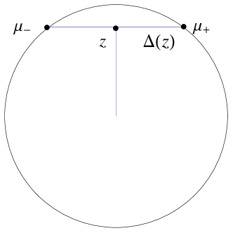
Figure 1. The median map and its inverse

In fact the formula for these points is

(2.6) $$\mu_{\pm}(z)=z\pm\Delta(z)\frac{z^{\perp}}{|z^{\perp}|}$$

where if $z=(x,y)$ then $z^{\perp}=(-y,x)$, and where we set (see Figure 1)

(2.7) $$\Delta(z)=\sqrt{\lambda^{2}-|z|^{2}}=\frac{1}{2}|\mu_{+}(z)-\mu_{-}(z)|$$

Let $\mathcal{Z}=\mathcal{Z}_{\lambda}$ be the set of medians of integer points with $|\mu|=\lambda$. Note that $\#\mathcal{Z}\leq(\#\mathcal{E})^{2}\ll\lambda^{o(1)}$.

Lemma 2.2.

Given vectors $z,v\in{\mathbb{R}}^{2}$, the number of $w\in\mathcal{Z}_{\lambda}$ for which

(2.8) $$|\mu_{+}(w)-v|<\sqrt{\lambda}$$

and

(2.9) $$|w-z|<\lambda^{1/3}$$

is at most $O(B_{\lambda})$.

Proof.

The medians $w$ satisfying (2.8) have their corresponding lattice points $\mu_{+}(w)$ each lying in an arc of length about $\sqrt{\lambda}$, and hence there are at most $B_{\lambda}$ possibilities for $\mu_{+}(w)$. Given $\mu_{+}(w)$, we have at most $2$ possibilities for $\mu_{-}(w)$: Indeed, since $w=(\mu_{+}(w)+\mu_{-}(w))/2$, we have

(2.10) $$\mu_{-}(w)=2w-\mu_{+}(w)=2z-\mu_{+}(w)+2(w-z)$$

Since $|w-z|<\lambda^{1/3}$, given $z$ and $\mu_{+}(w)$ we know $\mu_{-}(w)$ up to an error of $O(\lambda^{1/3})$; by Jarnik’s theorem, which states that an arc of size $\lambda^{1/3}$ contains at most two lattice points, this implies there are at most two possibilities for $\mu_{-}(w)$.

Since $w=(\mu_{+}(w)+\mu_{-}(w))/2$ is determined by knowing both $\mu_{\pm}(w)$, we see that there are at most $O(B_{\lambda})$ possibilities for $w$. ∎

3. An oscillatory integral along the curve

3.1. Phase functions on the curve

Let ${\mathbb{T}}^{2}={\mathbb{R}}^{2}/2\pi{\mathbb{Z}}^{2}$ be the standard flat torus. An eigenfunction $F$ of the Laplacian on ${\mathbb{T}}^{2}$ with eigenvalue $\lambda^{2}$ has a Fourier expansion

(3.1) $$F(x)=\sum_{\mu\in\mathcal{E}}a_{\mu}e^{i\langle\mu,x\rangle}$$

For $F$ to be real valued forces $\overline{a_{\mu}}=a_{-\mu}$. The supremum of $F$ is bounded by

(3.2) $$||F||_{\infty}\leq\sum_{\mu\in\mathcal{E}}|a_{\mu}|\leq\frac{1}{2\pi}||F||_{2}\sqrt{\#\mathcal{E}}$$

We normalize so that

(3.3) $$4\pi^{2}||F||_{2}^{2}=\sum_{\mu\in\mathcal{E}}|a_{\mu}|^{2}=1$$

Let $\gamma:[0,L]\to\mathcal{C}$ be an arc-length parameterization of $\mathcal{C}$, so that $\gamma^{\prime}(t)$ is the unit tangent vector to the curve at the point $\gamma(t)$. Denote by $n(t)$ the standard unit normal to the curve at the point $\gamma(t)$, so that $\gamma^{\prime\prime}(t)=\kappa(t)n(t)$ with $\kappa(t)$ the curvature. Let $K_{\min}>0$ and $K_{\max}$ be the minimum and maximum values of the curvature, so that

(3.4) $$0<K_{\min}\leq\kappa(t)\leq K_{\max}$$

By shrinking the curve $\mathcal{C}$, we may assume that its total curvature is $<\pi/2$.

We denote $f(t)=F(\gamma(t))$. Using the Fourier expansion of $F$, we write

(3.5) $$f(t)=\sum_{\mu\in\mathcal{E}}a_{\mu}e^{i\langle\mu,\gamma(t)\rangle}=\sum_{\mu\in\mathcal{E}}a_{\mu}e^{i\lambda\phi_{\mu}(t)}$$

where the phase function $\phi_{\mu}$ is

(3.6) $$\phi_{\mu}(t)=\langle\frac{\mu}{|\mu|},\gamma(t)\rangle$$

The derivative of $\phi_{\mu}$ is

(3.7) $$\phi^{\prime}_{\mu}(t)=\langle\frac{\mu}{|\mu|},\gamma^{\prime}(t)\rangle=\sin\alpha_{\mu}(t)$$

where $\alpha_{\mu}(t)$ is the angle between the normal vector $n(t)$ and $\mu$. Since we assume the total curvature of the curve is $<\pi/2$, the change in the angle $\alpha_{\mu}$ is less than $\pi/2$. The second derivative is

(3.8) $$\phi^{\prime\prime}_{\mu}(t)=\langle\frac{\mu}{|\mu|},\gamma^{\prime\prime}(t)\rangle=\kappa(t)\cos\alpha_{\mu}(t)$$

By (3.4),

(3.9) $$|\phi^{\prime\prime}_{\mu}|\leq K_{\max}$$

The third derivative is

(3.10) $$\phi_{\mu}^{\prime\prime\prime}=\langle\frac{\mu}{|\mu|},\gamma^{\prime\prime\prime}\rangle=\langle\frac{\mu}{|\mu|},\kappa^{\prime}n+\kappa n^{\prime}\rangle=\langle\frac{\mu}{|\mu|},\kappa^{\prime}n-\kappa^{2}\gamma^{\prime}\rangle$$

(since $n^{\prime}=-\kappa\gamma^{\prime}$) and hence, since $n\perp\gamma^{\prime}$,

(3.11) $$|\phi_{\mu}^{\prime\prime\prime}|\leq(|\kappa^{\prime}|_{\infty}^{2}+K_{\max}^{4})^{1/2}$$

is bounded independent of $\mu$.

Lemma 3.1.

For $0<\sigma\ll 1$ sufficiently small, let $B_{\mu}$ be the set of points where $|\phi^{\prime}_{\mu}(t)|<2\sigma$. Then $B_{\mu}$ is an interval and

(3.12) $$\operatorname{length}B_{\mu}\ll\frac{\sigma}{K_{\min}}$$

Proof.

We have

(3.13) $$|\phi^{\prime}_{\mu}(t)|=|\langle\frac{\mu}{|\mu|},\gamma^{\prime}(t)\rangle|=|\sin\alpha_{\mu}(t)|<2\sigma$$

Since we assume the total curvature is $<\pi/2$, the change in the angle $\alpha_{\mu}$ is less than $\pi/2$ and hence $B_{\mu}=(c_{,}c_{+})$ consists of at most a single interval.

Since $B_{\mu}$ is in particular connected and

$$|\phi^{\prime\prime}_{\mu}(t)|=\kappa(t)|\cos\alpha_{\mu}|\geq K_{\min}\sqrt{1-4\sigma^{2}}\geq K_{\min}/2$$

on $B_{\mu}$, we may assume that $\phi^{\prime\prime}_{\mu}\geq K_{\min}/2>0$ on $B_{\mu}$ so that $\phi^{\prime}_{\mu}$ is monotonically increasing. Then $\phi^{\prime}_{\mu}(c_{-})\geq-2\sigma$, $\phi^{\prime}_{\mu}(c_{+})\leq+2\sigma$ and we have

(3.14) $$4\sigma\geq\phi_{\mu}^{\prime}(c_{+})-\phi_{\mu}^{\prime}(c_{-})=(c_{+}-c_{-})\phi^{\prime\prime}_{\mu}(c)$$

for some $c\in(c_{-},c_{+})$ and hence

(3.15) $$\operatorname{length}B_{\mu}=c_{+}-c_{-}\leq\frac{4\sigma}{\phi^{\prime\prime}_{\mu}(c)}\leq\frac{8\sigma}{K_{\min}}$$

as claimed. ∎

3.2. Van der Corput’s lemma

Let $[a,b]$ be a finite interval, $\phi\in C^{\infty}[a,b]$ a smooth and real valued phase function, and $A\in C^{\infty}[a,b]$ a smooth amplitude. For $\lambda>0$ define the oscillatory integral

(3.16) $$I(\lambda):=\int_{a}^{b}A(t)e^{i\lambda\phi(t)}dt$$

We will need the following well-known result, due to van der Corput (see e.g. [12])

Lemma 3.2.

Assume that $|\phi^{\prime\prime}|\geq 1$. Then

(3.17) $$|I(\lambda)|\ll\frac{1}{\lambda^{1/2}}\left\{||A||_{\infty}+||A^{\prime}||_{1}\right\}$$

If $|\phi^{\prime}|\geq 1$ and moreover $\phi^{\prime}$ is monotonic then

(3.18) $$|I(\lambda)|\ll\frac{1}{\lambda}\left\{||A||_{\infty}+||A^{\prime}||_{1}\right\}$$

the implied constants absolute.

3.3. An oscillatory integral along a curve

For each $0\neq\xi\in{\mathbb{R}}^{2}$ define a phase function on the curve $\mathcal{C}$ by

(3.19) $$\phi_{\xi}(t)=\langle\frac{\xi}{|\xi|},\gamma(t)\rangle$$

Let $A\in C^{\infty}[0,L]$ be a smooth amplitude, $k$ real and

(3.20) $$I(k)=\int A(t)e^{ik\phi_{\xi}(t)}dt\;.$$

Lemma 3.3.

For $|k|\geq 1$,

(3.21) $$|I(k)|\ll\frac{1}{|k|^{1/2}}\left\{||A||_{\infty}+||A^{\prime}||_{1}\right\}\;,$$

the implied constant depending only on the curve $\mathcal{C}$ (independent of $\xi$).

Proof.

We wish to apply Lemma 3.2. Since the total curvature of $\mathcal{C}$ is $<\pi/2$, each of the phase functions $\phi_{\xi}$ has at most one stationary point (at a point where $\xi$ is normal to the curve). Moreover $\phi_{\xi}^{\prime\prime}(t)=\kappa(t)\cos\alpha_{\xi}(t)$ has at most one sign change since we restrict the total curvature to be $<\pi/2$.

Near a stationary point $t_{0}$, we have $|\phi^{\prime}_{\xi}(t)|<1/2$ if $|t-t_{0}|<1/(2K_{\max})$, since

(3.22) $$|\phi_{\xi}^{\prime}(t)|=|\phi_{\xi}^{\prime}(t)-\phi_{\xi}^{\prime}(t_{0})|=|t-t_{0}|\cdot|\phi_{\xi}^{\prime\prime}(t_{1})|\leq K_{\max}|t-t_{0}|$$

If $|\phi^{\prime}_{\xi}(t)|<1/2$, then

(3.23) $$|\phi_{\xi}^{\prime\prime}(t)|=\kappa(t)|\cos\alpha_{\xi}(t)|=\kappa(t)\sqrt{1-\phi_{\xi}^{\prime}(t)^{2}}\geq K_{\min}\frac{\sqrt{3}}{2}$$

Hence we may cut the curve, that is the arc-length parameter interval $[0,L]$, into at most $4$ segments on each of which either $|\phi_{\xi}^{\prime\prime}|\geq\frac{\sqrt{3}}{2}K_{\min}>0$ or $|\phi_{\xi}^{\prime}|\geq 1/2$ and $\phi_{\xi}^{\prime\prime}$ does not change sign, hence $\phi_{\xi}^{\prime}$ is monotonic. Then we can invoke Lemma 3.2 to deduce that either (3.18) or (3.17) hold, and since $|k|\geq 1$ we have (3.17) valid in both cases. ∎

4. A bilinear inequality on the curve

As before let $\mathcal{E}=\{\mu\in{\mathbb{Z}}^{2}:|\mu|=\lambda\}$. For each $\mu\in\mathcal{E}$ let $h_{\mu}(t)\in C_{c}^{1}({\mathbb{R}})$ and $a_{\mu}\in{\mathbb{C}}$ with $\sum_{\mu\in\mathcal{E}}|a_{\mu}|^{2}=1$. Let

(4.1) $$H(t):=\sum_{\mu\in\mathcal{E}}a_{\mu}h_{\mu}(t)e^{i\langle\mu,\gamma(t)\rangle}$$

Lemma 4.1.

(4.2) $$||H||_{2}^{2}\leq 2\max_{\mu\in\mathcal{E}}||h_{\mu}||_{2}^{2}+O(\frac{\#\mathcal{E}}{\lambda^{1/6}}\left\{\max_{\mu\in\mathcal{E}}||h_{\mu}||_{\infty}^{2}+\max_{\mu\in\mathcal{E}}||h_{\mu}||_{\infty}\max_{\mu\in\mathcal{E}}||h_{\mu}^{\prime}||_{1}\right\})$$

Proof.

Multiplying out gives

(4.3) $$||H||_{2}^{2}=\sum_{\mu,\nu}a_{\mu}\bar{a}_{\nu}\int h_{\mu}(t)\overline{h_{\nu}(t)}e^{i|\mu-\nu|\phi_{\mu-\nu}(t)}dt$$

where if $\mu=\nu$ we set $\phi_{0}(t)\equiv 1$. We separate the double sum (4.3) to a sum over ”close” pairs $(\mu,\nu)$, that is such that $|\mu-\nu|<\lambda^{1/3}$, and to a sum over the remaining ”distant” pairs. We claim that the ”close” pairs contribute

(4.4) $$\mbox{close }\leq 2\max_{\mu\in\mathcal{E}}||h_{\mu}||_{2}^{2}$$

while the ”distant” pairs contribute at most

(4.5) $$\mbox{distant }\ll\frac{\#\mathcal{E}}{\lambda^{1/6}}\left\{\max_{\mu\in\mathcal{E}}||h_{\mu}||_{\infty}^{2}+\max_{\mu\in\mathcal{E}}||h_{\mu}||_{\infty}\max_{\mu\in\mathcal{E}}||h_{\mu}^{\prime}||_{1}\right\}$$

4.0.1. Close pairs

Given $\mu\in\mathcal{E}$, certainly we can take $\nu=\mu$ to get a ”close” pair. By Jarnik’s theorem [10], given $\mu\in\mathcal{E}$ there is at most one other element of $\mathcal{E}$ at distance $\leq\lambda^{1/3}$ from $\mu$, call it $\tilde{\mu}$ (if it exists). Estimating the integral trivially by

(4.6) $$\left|\int h_{\mu}(t)\overline{h_{\nu}(t)}e^{i\langle\mu-\nu,\gamma(t)\rangle}dt\right|\leq||h_{\mu}||_{2}\cdot||h_{\nu}||_{2}$$

we find that the contribution of ”close” pairs is bounded by

(4.7) $$\max_{\mu}||h_{\mu}||_{2}^{2}\cdot\sum_{\mu\in\mathcal{E}}|a_{\mu}|^{2}+|a_{\mu}||a_{\tilde{\mu}}|$$

If $\mu$ does not have a close neighbor other than itself, the term $a_{\mu}a_{\tilde{\mu}}$ is zero. Otherwise, use $|a_{\mu}a_{\tilde{\mu}}|\leq\frac{1}{2}(|a_{\mu}|^{2}+|a_{\tilde{\mu}}|^{2})$. Since each $\mu$ has at most one such close neighbor $\tilde{\mu}$, the sum over all $\mu\in\mathcal{E}$ is at most

(4.8) $$\sum_{\mu\in\mathcal{E}}|a_{\mu}||a_{\tilde{\mu}}|\leq\sum_{\mu\in\mathcal{E}}\frac{1}{2}(|a_{\mu}|^{2}+|a_{\tilde{\mu}}|^{2})\leq\sum_{\mu\in\mathcal{E}}|a_{\mu}|^{2}=1$$

and hence

(4.9) $$\mbox{close }\leq 2\max_{\mu}||h_{\mu}||_{2}^{2}$$

4.0.2. Distant pairs

We now bound the contribution of pairs $\mu,\nu$ with $|\mu-\nu|>\lambda^{1/3}$ by

(4.10) $$\mbox{distant }\leq\sum_{|\mu-\nu|>\lambda^{1/3}}|a_{\mu}||a_{\nu}||I(\mu,\nu)|$$

where

(4.11) $$I(\mu,\nu):=\int h_{\mu}(t)\overline{h_{\nu}(t)}e^{i\langle\mu-\nu,\gamma(t)\rangle}dt=\int A_{\mu,\nu}(t)e^{i|\mu-\nu|\phi_{\mu-\nu}(t)}dt$$

where $A_{\mu,\nu}=h_{\mu}(t)\overline{h_{\nu}(t)}$.

By Lemma 3.3,

(4.12) $$\begin{split}|I(\mu,\nu)|&\ll\frac{1}{|\mu-\nu|^{1/2}}(||A_{\mu,\nu}||_{\infty}+||A^{\prime}_{\mu,\nu}||_{1})\\ &\ll\frac{1}{\lambda^{1/6}}\left\{\max_{\mu\in\mathcal{E}}||h_{\mu}||_{\infty}^{2}+\max_{\mu\in\mathcal{E}}||h_{\mu}||_{\infty}\max_{\mu\in\mathcal{E}}||h^{\prime}_{\mu}||_{1}\right\}\end{split}$$

Using (4.12) and $\sum_{\mu,\nu\in\mathcal{E}}|a_{\mu}a_{\nu}|\leq\#\mathcal{E}\sum_{\mu}|a_{\mu}|^{2}=\#\mathcal{E}$ we find that

(4.13) $$\begin{split}\mbox{distant }&\leq\sum_{\mu,\nu}|a_{\mu}||a_{\nu}|\max_{|\mu-\nu|>\lambda^{1/3}}I(\mu,\nu)\\ &\ll\frac{\#\mathcal{E}}{\lambda^{1/6}}\left\{\max_{\mu\in\mathcal{E}}||h_{\mu}||_{\infty}^{2}+\max_{\mu\in\mathcal{E}}||h_{\mu}||_{\infty}\max_{\mu\in\mathcal{E}}||h^{\prime}_{\mu}||_{1}\right\}\end{split}$$

as claimed. ∎

5. Proof of Theorem 1.2

5.1. Overview

We denote $f(t)=F(\gamma(t))$, which is real valued, and want to count zeros of $f$ on $[0,L]$. The idea is to detect sign changes of $f$ by comparing $\int|f|$ and $|\int f|$.

Let $C_{1}$ be a parameter, which we will want to satsify $1\ll C_{1}=o(\lambda)$, and consider a partition of unity $\{\tau_{j}\}_{j\in J}$ of the interval $[0,L]$, where $\tau_{j}\geq 0$, $\sum_{j}\tau_{j}=\mathbf{1}_{[0,L]}$, so that

1. $\#J\approx\lambda/C_{1}$

2. $\tau_{j}$ supported in an interval of length $\approx C_{1}/\lambda$

3. $|\partial^{r}\tau_{j}/\partial t^{r}|\ll(\lambda/C_{1})^{r}$

4. for each $j$, there is at most $O(1)$ values of $k$ for which $\tau_{j}\tau_{k}\neq 0$ (independent of $\lambda$). In particular for each point $t$ there is at most $O(1)$ values of $j$ so that $\tau_{j}(t)\neq 0$.

Let $J_{0}\subseteq J$ be the set of indices $j$ for which $f$ has a sign change on $\operatorname{supp}\tau_{j}$. Since for each point $t$ there is at most $O(1)$ values of $j$ for which $t\in\operatorname{supp}\tau_{j}$, we have

(5.1) $$\#\mbox{ sign changes of }f\gg\#J_{0}$$

so that a lower bound for $\#J_{0}$ gives a lower bound for the number of sign changes of $f$.

If $j\notin J_{0}$ then $f\tau_{j}$ does not change sign and hence

(5.2) $$\int|f|\tau_{j}=|\int f\tau_{j}|,\quad j\notin J_{0}$$

Therefore

(5.3) $$\int|f|=\sum_{j}\int|f|\tau_{j}=\sum_{j\notin J_{0}}|\int f\tau_{j}|+\int|f|\sum_{j\in J_{0}}\tau_{j}$$

We will show that

(5.4) $$\int|f|\sum_{j\in J_{0}}\tau_{j}\ll(\frac{\#J_{0}C_{1}}{\lambda})^{1/2}$$

and that

(5.5) $$\sum_{j\notin J_{0}}|\int f\tau_{j}|\ll C_{1}^{-1/3}$$

so that

(5.6) $$\int|f|\ll(\frac{\#J_{0}C_{1}}{\lambda})^{1/2}+C_{1}^{-1/3}$$

Taking $C_{1}^{-1/3}=\delta\int|f|$ with $\delta>0$ sufficiently small gives

(5.7) $$\#J_{0}\gg\lambda(\int|f|)^{5}$$

which proves Theorem 1.2. Note that our choice of $C_{1}$ indeed satisfies our requirements, indeed $1\ll C_{1}\ll\lambda^{o(1)}$ since $\int|f|\ll(\int|f|^{2})^{1/2}\ll||F||_{2}\approx 1$, by the upper bound in the uniform $L^{2}$-restriction theorem [1], and $\int|f|\gg\lambda^{-o(1)}$ from the lower bound in the uniform $L^{2}$-restriction theorem, see (6.3).

5.2. Proof of (5.4)

By Cauchy-Schwarz,

(5.8) $$\int|f|\sum_{j\in J_{0}}\tau_{j}\leq||f||_{2}\{\int(\sum_{j\in J_{0}}\tau_{j})^{2}\}^{1/2}=||f||_{2}\{\sum_{j,k\in J_{0}}\int\tau_{j}\tau_{k}\}^{1/2}$$

By the restriction upper bound of [1], $||f||_{2}\ll 1$. Given $j$, we have $\int\tau_{j}\tau_{k}=0$ except for $O(1)$ indices $k$ (independent of $j$), including $k=j$, and for such $k$ we have

(5.9) $$\int\tau_{j}\tau_{k}\leq\frac{1}{2}(\int\tau_{j}^{2}+\int\tau_{k}^{2})\leq\max_{k}\int\tau_{k}^{2}$$

Since

(5.10) $$\int\tau_{k}^{2}\leq\int_{\operatorname{supp}\tau_{k}}1\ll\frac{C_{1}}{\lambda}$$

we obtain

(5.11) $$\int(\sum_{j\in J_{0}}\tau_{j})^{2}\ll\#J_{0}\max_{k}\int\tau_{k}^{2}\ll\frac{\#J_{0}C_{1}}{\lambda}$$

and hence

(5.12) $$\sum_{j\in J_{0}}\int|f|\tau_{j}\ll(\frac{\#J_{0}C_{1}}{\lambda})^{1/2}$$

5.3. Proof of (5.5)

Our goal is to show that

(5.13) $$\sum_{j\notin J_{0}}\left|\int f(t)\tau_{j}(t)dt\right|$$

is small.

Let $\sigma>0$ be a (small) parameter, $\lambda^{-o(1)}<\sigma<1$ and $0\leq\theta(x)\leq 1$ a smooth, even function so that $\theta(x)=1$ if $|x|<1$, $\theta(x)=0$ for $|x|>2$ and set $\theta_{\sigma}(x)=\theta(\frac{x}{\sigma})$.

Write $f=f_{0}+f_{1}$ where

(5.14) $$f_{0}(t)=\sum_{\mu\in\mathcal{E}}a_{\mu}\theta_{\sigma}(\phi^{\prime}_{\mu}(t))e^{i\lambda\phi_{\mu}(t)}$$

and

(5.15) $$f_{1}(t)=\sum_{\mu\in\mathcal{E}}a_{\mu}(1-\theta_{\sigma})(\phi^{\prime}_{\mu}(t))e^{i\lambda\phi_{\mu}(t)}$$

Thus in the Fourier expansion of $f_{1}$, none of the phase functions $\phi_{\mu}$ have a critical point in the support of $(1-\theta_{\sigma})\phi^{\prime}_{\mu}$, in fact they satisfy $|\phi^{\prime}_{\mu}(t)|\geq\sigma$.

We have

(5.16) $$\sum_{j\notin J_{0}}\left|\int f(t)\tau_{j}(t)dt\right|\leq\sum_{j\notin J_{0}}\left|\int f_{0}(t)\tau_{j}(t)dt\right|+\sum_{j\notin J_{0}}\left|\int f_{1}(t)\tau_{j}(t)dt\right|$$

We will show that

(5.17) $$\sum_{j\notin J_{0}}\left|\int f_{0}(t)\tau_{j}(t)dt\right|\ll\sigma^{1/2}$$

and

(5.18) $$\sum_{j\notin J_{0}}\left|\int f_{1}(t)\tau_{j}(t)dt\right|\ll\frac{1}{C_{1}\sigma}$$

which gives

(5.19) $$\sum_{j\notin J_{0}}|\int f\tau_{j}|\ll\sigma^{1/2}+\frac{1}{C_{1}\sigma}$$

Choosing $C_{1}=\sigma^{-3/2}$ gives

(5.20) $$\sum_{j\notin J_{0}}|\int f\tau_{j}|\ll C_{1}^{-1/3}$$

proving (5.5).

5.4. Proof of (5.17)

We have

(5.21) $$\sum_{j\notin J_{0}}\left|\int f_{0}(t)\tau_{j}(t)dt\right|\leq\int|f_{0}(t)|dt\ll||f_{0}||_{2}$$

and hence (5.17) follows from:

Lemma 5.1.

(5.22) $$||f_{0}||_{2}\ll\sigma^{1/2}$$

Proof.

We wish to apply Lemma 4.1 with $h_{\mu}=\theta(\frac{\phi_{\mu}^{\prime}}{\sigma})$. We clearly have $||h_{\mu}||_{\infty}\leq 1$. Moreover,

(5.23) $$||h_{\mu}||_{2}^{2}\leq\int\theta(\frac{\phi^{\prime}}{\sigma})\leq\operatorname{length}\{t:|\phi^{\prime}_{\mu}(t)|<2\sigma\}$$

and hence $||h_{\mu}||_{2}^{2}\ll\sigma$ by Lemma 3.1. Likewise

(5.24) $$||h^{\prime}_{\mu}||_{1}=\int|\theta^{\prime}(\frac{\phi^{\prime}_{\mu}}{\sigma})|\frac{|\phi_{\mu}^{\prime\prime}|}{\sigma}\leq\frac{K_{\max}|\theta^{\prime}|_{\infty}}{\sigma}\operatorname{length}\{t:|\phi^{\prime}_{\mu}(t)|<2\sigma\}$$

and hence $||h^{\prime}_{\mu}||_{1}\ll 1$. Inserting into Lemma 4.1 gives

(5.25) $$||f_{0}||_{2}^{2}\ll\sigma+\frac{\#\mathcal{E}}{\lambda^{1/6}}$$

which gives our claim provided $\sigma\gg\lambda^{-o(1)}$. ∎

5.5. Proof of (5.18)

We expand and integrate by parts

(5.26) $$\int f_{1}\tau_{j}=\frac{1}{i\lambda}\int f_{2}\tau_{j}+\frac{1}{i\lambda}\int f_{3}\tau^{\prime}_{j}$$

where

(5.27) $$f_{2}=\sum_{\mu\in\mathcal{E}}a_{\mu}\left(\frac{1-\theta_{\sigma}(\phi^{\prime}_{\mu})}{\phi^{\prime}_{\mu}}\right)^{\prime}e^{i\lambda\phi_{\mu}}$$

and

(5.28) $$f_{3}=\sum_{\mu\in\mathcal{E}}a_{\mu}\frac{1-\theta_{\sigma}(\phi^{\prime}_{\mu})}{\phi^{\prime}_{\mu}}e^{i\lambda\phi_{\mu}}$$

Hence

(5.29) $$\begin{split}\sum_{j\notin J_{0}}|\int f_{1}\tau_{j}|&\leq\frac{1}{\lambda}\left(\int|f_{2}|\sum_{j\notin J_{0}}\tau_{j}+\int|f_{3}|\sum_{j\notin J_{0}}|\tau^{\prime}_{j}|\right)\\ &\leq\frac{1}{\lambda}||f_{2}||_{2}+\frac{1}{\lambda}||f_{3}||_{2}\left\{\int(\sum_{j\notin J_{0}}|\tau^{\prime}_{j}|)^{2}\right\}^{1/2}\end{split}$$

We have

(5.30) $$\int(\sum_{j\notin J_{0}}|\tau^{\prime}_{j}|)^{2}=\sum_{j\notin J_{0}}\sum_{k\notin J_{0}}\int|\tau^{\prime}_{j}\tau^{\prime}_{k}|\ll\sum_{j\notin J_{0}}\int(\tau^{\prime}_{j})^{2}$$

since for each $j$, there are only $O(1)$ values of $k$ for which $\tau^{\prime}_{j}\tau^{\prime}_{k}\neq 0$. Hence

(5.31) $$\int(\sum_{j\notin J_{0}}|\tau^{\prime}_{j}|)^{2}\ll\sum_{j\notin J_{0}}\int(\tau^{\prime}_{j})^{2}\ll(\frac{\lambda}{C_{1}})^{2}$$

Therefore

(5.32) $$\sum_{j\notin J_{0}}|\int f_{1}\tau_{j}|\ll\frac{1}{\lambda}||f_{2}||_{2}+\frac{1}{C_{1}}||f_{3}||_{2}$$

Using Lemma 4.1 we find

(5.33) $$||f_{2}||_{2}\ll\frac{1}{\sigma^{2}}\;,\quad||f_{3}||_{2}\ll\frac{1}{\sigma}$$

once we note that

(5.34) $$|\frac{1-\theta_{\sigma}(\phi^{\prime}_{\mu})}{\phi^{\prime}_{\mu}}|\ll\frac{1}{\sigma}$$

(5.35) $$|\left\{\frac{1-\theta_{\sigma}(\phi^{\prime}_{\mu})}{\phi^{\prime}_{\mu}}\right\}^{\prime}|\ll\frac{1}{\sigma^{2}}$$

and, using (3.11), that

(5.36) $$|\left\{\frac{1-\theta_{\sigma}(\phi^{\prime}_{\mu})}{\phi^{\prime}_{\mu}}\right\}^{\prime\prime}|\ll\frac{1}{\sigma^{3}}$$

(we assume throughout that $\sigma\gg\lambda^{-o(1)}$). This gives

(5.37) $$\sum_{j\notin J_{0}}|\int f_{1}\tau_{j}|\ll\frac{1}{\lambda}\frac{1}{\sigma^{2}}+\frac{1}{C_{1}}\frac{1}{\sigma}\ll\frac{1}{C_{1}\sigma}$$

proving (5.18).

6. Relating $L^{1}$ and $L^{4}$ restriction theorems

We briefly explain the relation between $L^{1}$ and $L^{4}$ restriction theorems given in (1.9), namely

(6.1) $$||F||_{L^{1}(\mathcal{C})}\gg_{\mathcal{C}}\frac{||F||_{2}^{3}}{||F||^{2}_{L^{4}(\mathcal{C})}}$$

By Cauchy-Schwarz, $\int_{\mathcal{C}}|F|\ll||F||_{L^{2}(\mathcal{C})}$ and by the upper bound in the $L^{2}$-restriction theorem [1] we have $||F||_{L^{2}(\mathcal{C})}\ll||F||_{2}$ so that

(6.2) $$\int_{\mathcal{C}}|F|\ll||F||_{2}$$

As for lower bounds, we certainly have $\int_{\mathcal{C}}|F|^{2}\leq||F||_{\infty}\int_{\mathcal{C}}|F|$ and combining the lower bound in the $L^{2}$-restriction theorem [1], $\int_{\mathcal{C}}|F|^{2}\gg||F||_{2}^{2}$ with the upper bound on the $L^{\infty}$ norm $||F||_{\infty}\leq\sqrt{\#\mathcal{E}}||F||_{2}/2\pi$ (see (3.2)) we obtain

(6.3) $$\frac{1}{||F||_{2}}\int_{\mathcal{C}}|F|\gg\frac{1}{\sqrt{\#\mathcal{E}}}$$

We want to improve the bound (6.3) for $\int_{\mathcal{C}}|F|$. To start with, we use interpolation (log-convexity of the $L^{p}$ norm) to give a lower bound for $||F||_{L^{1}(\mathcal{C})}=\int_{\mathcal{C}}|F|$ in terms of the $L^{2}$ and $L^{4}$ norms on the curve:

(6.4) $$||F||_{L^{2}(\mathcal{C})}\leq||F||_{L^{1}(\mathcal{C})}^{1/3}\cdot||F||_{L^{4}(\mathcal{C})}^{2/3}$$

which improves on (6.3) as it does not contain any component which is a-priori unbounded in $\lambda$.

Inserting the uniform $L^{2}$ restriction lower bound $||F|||_{L^{2}(\mathcal{C})}\gg||F||_{2}$ of [1] into (6.4) gives (6.1) as claimed.

7. An upper bound on the restriction $L^{4}$ norm: Proof of Theorem 1.3

The aim of this section is to reduce getting a uniform upper bound for the $4$-th moment $\int_{\mathcal{C}}|F|^{4}$, to counting lattice points in arcs of length $\sqrt{\lambda}$ by showing that

(7.1) $$\int_{\mathcal{C}}|F|^{4}=\int|f(t)|^{4}dt\ll B_{\lambda}$$

where as in (1.6),

(7.2) $$B_{\lambda}=\max_{|x|=\lambda}\#\{\xi\in\mathcal{E}:|x-\xi|\leq\sqrt{\lambda}\}$$

7.1. Computing $\int|f|^{4}$

Recall

(7.3) $$f(t)=\sum_{\mu}a_{\mu}e^{i\langle\mu,\gamma(t)\rangle}$$

We may break up $f$ into $O(1)$ terms, each the sum over frequencies $\mu$ lying in an arc of size $\lambda/100$. By the triangle inequality, it suffices to prove the restriction $L^{4}$ bound for such $f$, and from now on we assume that $f$ is of this form.

In order to compute the $4$-th moment $\int|f|^{4}$, write

(7.4) $$f(t)^{2}=\sum_{\mu,\nu}a_{\mu}a_{\nu}e^{i\langle\mu+\nu,\gamma(t)\rangle}=\sum_{\mu}a_{\mu}a_{-\mu}+\sum_{0\neq z\in\mathcal{Z}}b_{z}e^{2i\langle z,\gamma(t)\rangle}$$

where for a median $z=(\mu+\nu)/2\in\mathcal{Z}$ (see § 2.2), we set $b_{z}=2a_{\mu}a_{\nu}$. The assumption that all the frequencies $\mu$ lie in an arc of size $\lambda/100$ implies that the medians $z\in\mathcal{Z}$ appearing in (7.4) satisfy $|z|>\lambda/2$, and that $a_{\mu}a_{-\mu}=0$ for all $\mu$. Observe that

(7.5) $$\sum_{0\neq z\in\mathcal{Z}}|b_{z}|^{2}\ll(\sum_{\mu}|a_{\mu}|^{2})^{2}=\frac{1}{(2\pi)^{4}}||F||_{2}^{4}$$

Hence we can we write

(7.6) $$f(t)^{2}=g_{0}(t)+g(t)$$

with

(7.7) $$g_{0}(t)=\sum_{0<\Delta(z)\leq\sqrt{\lambda}}b_{z}e^{2i\langle z,\gamma(t)\rangle}$$

and

(7.8) $$g(t)=\sideset{}{{}^{\ast}}{\sum}_{z}b_{z}e^{2i\langle z,\gamma(t)\rangle}$$

where we denote

(7.9) $$\sideset{}{{}^{\ast}}{\sum}_{z}:=\sum_{\begin{subarray}{c}z\in\mathcal{Z}\\ |z|\geq\lambda/2\\ |\Delta(z)|>\sqrt{\lambda}\end{subarray}}$$

Therefore

(7.10) $$||f||_{4}=||f^{2}||_{2}^{1/2}\leq\left(||g_{0}||_{2}+||g||_{2})\right)^{1/2}$$

so that it suffices to show

(7.11) $$||g_{0}||_{2}^{2}\ll B_{\lambda}||b||^{2}\;,\qquad||g||_{2}^{2}\ll B_{\lambda}||b||^{2}$$

where $b=(b_{z})\in{\mathbb{C}}^{\mathcal{Z}}$.

By Lemma 3.3, if $z\neq w$ then

(7.12) $$\int e^{2i\langle z-w,\gamma(t)\rangle}dt\ll\frac{1}{|z-w|^{1/2}}$$

and since the integral is trivially bounded by $\ll 1$, we can write this for any pair $z,w\in\mathcal{Z}$ as

(7.13) $$\int e^{2i\langle z-w,\gamma(t)\rangle}dt\ll\frac{1}{|z-w|_{+}^{1/2}}$$

where

(7.14) $$|z|_{+}=\max\left(1,|z|\right)$$

Therefore

(7.15) $$\int|g|^{2}\ll\sideset{}{{}^{\ast}}{\sum}_{z}\sideset{}{{}^{\ast}}{\sum}_{w}\frac{|b_{z}||b_{w}|}{|z-w|_{+}^{1/2}}$$

Moreover, we may restrict the sum to $|w-z|<\lambda^{\epsilon}$ at a cost of $O(\lambda^{-\epsilon/2}||b||^{2}\#\mathcal{Z})=o(||F||_{2}^{4})$ since $\#\mathcal{Z}\ll\lambda^{o(1)}$. Denoting by

(7.16) $$\sideset{}{{}^{\ast}}{\sum}_{z,w}:=\sideset{}{{}^{\ast}}{\sum}_{z}\sideset{}{{}^{\ast}}{\sum}_{w:\;|z-w|<\lambda^{\epsilon}}$$

we have found that

(7.17) $$||g||^{2}\ll\sideset{}{{}^{\ast}}{\sum}_{z,w}\frac{|b_{z}b_{w}|}{|z-w|_{+}^{1/2}}$$

and likewise

(7.18) $$||g_{0}||^{2}\ll\sum_{\begin{subarray}{c}0<\Delta(z),\Delta(w)\leq\sqrt{\lambda}\\ |z-w|<\lambda^{\epsilon}\end{subarray}}\frac{|b_{z}b_{w}|}{|z-w|_{+}^{1/2}}$$

Thus we see that it suffices to show:

Proposition 7.1.

Let $b=(b_{z})\in{\mathbb{C}}^{\mathcal{Z}}$. Then

(i) $$\sum_{\begin{subarray}{c}0<\Delta(z),\Delta(w)<\sqrt{\lambda}\\ |z-w|<\lambda^{\epsilon}\end{subarray}}\frac{|b_{z}b_{w}|}{|z-w|_{+}^{1/2}}\ll B_{\lambda}||b||^{2}$$

and

(ii) $$\sideset{}{{}^{\ast}}{\sum}_{z,w}\frac{|b_{z}b_{w}|}{|z-w|_{+}^{1/2}}\ll B_{\lambda}||b||^{2}$$

7.2. Proof of Proposition 7.1 (i)

By Schur’s test,

(7.19) $$\sum_{\begin{subarray}{c}0<\Delta(z),\Delta(w)\leq\sqrt{\lambda}\\ |z-w|<\lambda^{\epsilon}\end{subarray}}\frac{|b_{z}b_{w}|}{|z-w|_{+}^{1/2}}\leq\max_{0<\Delta(z)\leq\sqrt{\lambda}}\sum_{\begin{subarray}{c}0<\Delta(w)\leq\sqrt{\lambda}\\ |z-w|<\lambda^{\epsilon}\end{subarray}}\frac{1}{|z-w|_{+}^{1/2}}||b||^{2}$$

and so it suffices to show that

(7.20) $$\sum_{\begin{subarray}{c}0<\Delta(w)\leq\sqrt{\lambda}\\ |z-w|<\lambda^{\epsilon}\end{subarray}}\frac{1}{|z-w|_{+}^{1/2}}\ll B_{\lambda}$$

Replacing $|z-w|_{+}$ by $1$ we are reduced to showing that

(7.21) $$\#\{0<\Delta(w)\leq\sqrt{\lambda},\quad|z-w|<\lambda^{\epsilon}\}\ll B_{\lambda}$$

We have

(7.22) $$\mu_{+}(w)-\mu_{+}(z)=(w-z)+(\Delta(w)-\Delta(z))\frac{z^{\perp}}{|z|}+\Delta(w)(\frac{w^{\perp}}{|w|}-\frac{z^{\perp}}{|z|})$$

Since $\Delta(z),\Delta(w)<\sqrt{\lambda}$ we have $|z|,|w|\sim\lambda$, and hence

(7.23) $$|\frac{w^{\perp}}{|w|}-\frac{z^{\perp}}{|z|}|\ll\frac{|z-w|}{\lambda}\ll\lambda^{-1+\epsilon}$$

Thus

(7.24) $$|\mu_{+}(w)-\mu_{+}(z)|\ll\sqrt{\lambda}$$

By Lemma 2.2 we see that there are at most $O(B_{\lambda})$ possibilities for $w$. This proves (7.21). ∎

7.3. A dyadic subdivision

We turn to the proof of part (ii) of Proposition 7.1. For $K\geq 1$, let

(7.25) $$S_{K}=\{z\in\mathcal{Z},\quad K\sqrt{\lambda}\leq\Delta(z)<2K\sqrt{\lambda}\}$$

We write

(7.26) $$\sideset{}{{}^{\ast}}{\sum}_{z,w}\frac{|b_{z}b_{w}|}{|z-w|_{+}^{1/2}}=\sum_{K,L\;\rm{dyadic}}\langle A_{K,L}b^{(K)},b^{(L)}\rangle\;,$$

the sum over $K=2^{k}$, $L=2^{\ell}$, with

(7.27) $$\langle A_{K,L}b^{(K)},b^{(L)}\rangle=\sideset{}{{}^{\ast}}{\sum}_{\begin{subarray}{c}w\in S_{L}\\ z\in S_{K}\end{subarray}}\frac{|b_{z}b_{w}|}{|z-w|_{+}^{1/2}}\;,$$

where $b^{(K)}=(|b_{z}|)_{z\in S_{K}}$, $b^{(L)}=(|b_{w}|)_{w\in S_{L}}$, and $A_{K,L}:{\mathbb{C}}^{S_{K}}\to{\mathbb{C}}^{S_{L}}$ is the matrix

(7.28) $$A_{K,L}=(\frac{1}{|z-w|_{+}^{1/2}})_{z\in S_{K},w\in S_{L}}$$

with zeros whenever one of the conditions $\Delta(z),\Delta(w)>\sqrt{\lambda}$, $|z|,|w|>\lambda/2$ or $|z-w|<\lambda^{\epsilon}$ is violated.

We use Schur’s test for the operator norm:

(7.29) $$||A_{K,L}||_{2\to 2}\leq||A_{K,L}||_{1\to 1}^{1/2}\cdot||A_{K,L}^{*}||_{1\to 1}^{1/2}$$

to bound

(7.30) $$|\langle A_{K,L}b^{(K)},b^{(L)}\rangle|\leq||A_{K,L}||_{1\to 1}^{1/2}\cdot||A_{K,L}^{*}||_{1\to 1}^{1/2}\cdot||b^{(K)}||\cdot||b^{(L)}||$$

where $||b^{(K)}||$ is the $\ell^{2}$-norm. We will show

Proposition 7.2.

For $K\leq L$,

(7.31) $$||A_{K,L}||_{1\to 1}\ll B_{\lambda}$$

and

(7.32) $$||A_{K,L}^{*}||_{1\to 1}\ll\frac{K}{L}B_{\lambda}$$

Therefore

(7.33) $$\begin{split}\sideset{}{{}^{\ast}}{\sum}_{z,w}\frac{|b_{z}b_{w}|}{|z-w|_{+}^{1/2}}&\ll B_{\lambda}\sum\sum_{K,L\;\rm{dyadic}}(\frac{\min(K,L)}{\max(K,L)})^{1/2}||b^{(K)}||\cdot||b^{(L)}||\\ &\ll B_{\lambda}\left\{\max_{K}\sum_{\begin{subarray}{c}L=2^{\ell}\;\rm{dyadic}\\ L\geq K\end{subarray}}(\frac{K}{L})^{1/2}\right\}\cdot\sum_{K}||b^{(K)}||^{2}\end{split}$$

Since $\sum_{K}||b^{(K)}||^{2}=||b||^{2}$ and

(7.34) $$\sum_{\begin{subarray}{c}L=2^{\ell}\;\rm{dyadic}\\ L\geq K\end{subarray}}(\frac{K}{L})^{1/2}\ll 1$$

we will have proved part (ii) in Proposition 7.1. ∎

7.4. Proof of Proposition 7.2

By Schur’s test,

(7.35) $$||A_{K,L}||_{1\to 1}\leq\max_{z\in S_{K}}\sideset{}{{}^{\ast}}{\sum}_{\begin{subarray}{c}w\in S_{L}\\ |z-w|<\lambda^{\epsilon}\end{subarray}}\frac{1}{|z-w|_{+}^{1/2}}$$

and

(7.36) $$||A_{K,L}^{*}||_{1\to 1}\leq\max_{w\in S_{L}}\sideset{}{{}^{\ast}}{\sum}_{\begin{subarray}{c}z\in S_{K}\\ |z-w|<\lambda^{\epsilon}\end{subarray}}\frac{1}{|z-w|_{+}^{1/2}}$$

Lemma 7.3.

Let $z\in S_{K}$. Then

(7.37) $$\#\{w\in S_{L}:|w-z|<\lambda^{\epsilon}\}\ll LB_{\lambda}$$

Proof.

For $0\leq l\leq L-1$, set

(7.38) $$S_{L,l}=\{w\in S_{L}:\quad(L+l)\sqrt{\lambda}\leq\Delta(w)<(L+l+1)\sqrt{\lambda}\}$$

We show that for $z\in S_{K}$, $w\in S_{L,l}$ and $|z-w|<\lambda^{\epsilon}$, we have

(7.39) $$|\mu_{+}(w)-v|\ll\sqrt{\lambda}$$

where

(7.40) $$v=\mu_{+}(z)+\left((L+l)\sqrt{\lambda}-\Delta(z)\right)\frac{z^{\perp}}{|z|}$$

By Lemma 2.2 we see that there are at most $O(B_{\lambda})$ possibilities for $w$ in $S_{L,l}$ subject to $|w-z|<\lambda^{\epsilon}$:

(7.41) $$\#\{w\in S_{L,l}:|w-z|<\lambda^{\epsilon}\}\ll B_{\lambda}$$

Since

(7.42) $$S_{L}=\bigcup_{l=0}^{L-1}S_{L,l}$$

we find

(7.43) $$\#\{w\in S_{L}:|w-z|<\lambda^{\epsilon}\}\ll LB_{\lambda}$$

as claimed.

To prove (7.39), we use (2.6) to get

(7.44) $$\mu_{+}(w)-\mu_{+}(z)=w-z+\Delta(w)\frac{w^{\perp}}{|w|}-\Delta(z)\frac{z^{\perp}}{|z|}$$

Note that $|w^{\perp}|=|w|$ and since $|z|\geq\lambda/2$ and $|z-w|<\lambda^{\epsilon}$ then $|w|=|z|+O(\lambda^{\epsilon})\gg\lambda$ and so

(7.45) $$\frac{w^{\perp}}{|w|}=\frac{z^{\perp}}{|z^{\perp}|}+O(\lambda^{-1+\epsilon})$$

Hence

(7.46) $$\begin{split}\mu_{+}(w)-\mu_{+}(z)&=O(\lambda^{\epsilon})+\Delta(w)(\frac{z^{\perp}}{|z^{\perp}|}+O(\lambda^{-1+\epsilon}))-\Delta(z)\frac{z^{\perp}}{|z^{\perp}|}\\ &=(\Delta(w)-\Delta(z))\frac{z^{\perp}}{|z^{\perp}|}+O(\lambda^{\epsilon})\end{split}$$

Writing $\Delta(w)=(L+l+\theta)\sqrt{\lambda}$ with $0\leq\theta<1$ we find

(7.47) $$\mu_{+}(w)-\mu_{+}(z)=\left((L+l)\sqrt{\lambda}-\Delta(z)\right)\frac{z^{\perp}}{|z^{\perp}|}+\theta\sqrt{\lambda}\frac{z^{\perp}}{|z^{\perp}|}+O(\lambda^{\epsilon})$$

proving (7.39). ∎

We now give a lower bound for the difference of medians $|z-w|$:

Lemma 7.4.

Let $K\leq L$, $w\in S_{L,l}$, $z\in S_{K,k}$, $0<|w-z|<\lambda^{\epsilon}$. Then

1. If $2K<L$ then $|z-w|\gg L^{2}$;

2. If $K=L/2$ and $l\neq 0$ then $|z-w|\gg Ll$ ;

3. If $K=L$ and $l\neq k,k\pm 1$ then $|z-w|\gg L|l-k|$.

Proof.

To bound $|z-w|$, the condition $K\leq L$ allows us to assume $|z|\geq|w|$. Then

(7.48) $$\begin{split}|z-w|&\geq|z|-|w|=\frac{\lambda^{2}-|w|^{2}}{\lambda+|w|}-\frac{\lambda^{2}-|z|^{2}}{\lambda+|z|}\\ &\geq\frac{\Delta(w)^{2}}{\lambda+|z|}-\frac{\Delta(z)^{2}}{\lambda+|z|}\\ &\geq\frac{\Delta(w)^{2}-\Delta(z)^{2}}{2\lambda}\\ &\gg\frac{L}{\sqrt{\lambda}}|\Delta(w)-\Delta(z)|\gg L(L+l-K-k-1)\end{split}$$

If $K\leq L/4$ then $L(L+l-K-k-1)\geq L(L-2K)\geq L^{2}/2$. If $K=L/2$ then $L|L+l-K-k-1|\geq L(L+l-2K)=Ll$, useful if $l\neq 0$. Finally if $K=L$ then $L(L+l-K-k-1|=L|l-k-1|\geq\frac{1}{2}L|l-k|$ if $|l-k|\geq 2$, the exceptional cases being $l=k,k\pm 1$. ∎

7.5. Bounding $||A_{K,L}||_{2\to 2}$

We want to show that, if $K\leq L$, then

(7.49) $$||A_{K,L}||_{1\to 1}\leq\max_{z\in S_{K}}\sum_{\begin{subarray}{c}w\in S_{L}\\ |z-w|<\lambda^{\epsilon}\end{subarray}}\frac{1}{|z-w|_{+}^{1/2}}\ll B_{\lambda}$$

and

(7.50) $$||A_{K,L}^{*}||_{1\to 1}\leq\max_{w\in S_{L}}\sum_{\begin{subarray}{c}z\in S_{K}\\ |z-w|<\lambda^{\epsilon}\end{subarray}}\frac{1}{|z-w|_{+}^{1/2}}\leq\frac{K}{L}B_{\lambda}$$

We assume first that $2K<L$, that is $K=2^{k}$, $L=2^{\ell}$ with $\ell\geq k+2$. Let

(7.51) $$S_{L}(z,\lambda^{\epsilon})=\{w\in S_{L}:|w-z|<\lambda^{\epsilon}\}$$

We have

(7.52) $$\begin{split}||A_{K,L}||_{1\to 1}&\leq\max_{z\in S_{K}}\sum_{w\in S_{L}(z,\lambda^{\epsilon})}\frac{1}{|z-w|_{+}^{1/2}}\\ &\leq\max_{z\in S_{K}}\frac{\#S_{L}(z,\lambda^{\epsilon})}{\min_{w\in S_{L}(z,\lambda^{\epsilon})}|z-w|_{+}^{1/2}}\end{split}$$

According to Lemma 7.3,

(7.53) $$\#S_{L}(z,\lambda^{\epsilon})\ll LB_{\lambda}$$

and by Lemma 7.4, if $2K<L$ then

(7.54) $$\min_{w\in S_{L}(z,\lambda^{\epsilon})}|z-w|\gg L^{2}$$

Hence we find (for $2K<L$)

(7.55) $$||A_{K,L}||_{1\to 1}\ll B_{\lambda}$$

Arguing in the same way with the roles of $L$ and $K$ reversed gives, for $2K<L$, that

(7.56) $$||A_{K,L}^{*}||_{1\to 1}\leq\max_{z\in S_{K}}\frac{\#S_{K}(z,\lambda^{\epsilon})}{\min_{w\in S_{K}(z,\lambda^{\epsilon})}|z-w|_{+}^{1/2}}\leq\frac{KB_{\lambda}}{L}$$

7.6. The cases $K=L/2,L$

It remains to deal with the case $K=L/2$ and $K=L$. We use the decomposition $S_{L}=\bigcup_{l=0}^{L-1}S_{L,l}$ in (7.38) to write

(7.57) $$\begin{split}\sum_{w\in S_{L}(z,\lambda^{\epsilon})}\frac{1}{|z-w|_{+}^{1/2}}&\ll\sum_{l=0}^{L-1}\sum_{w\in S_{L,l}(z,\lambda^{\epsilon})}\frac{1}{|z-w|_{+}^{1/2}}\\ &\ll\sum_{l=0}^{L-1}\frac{\#S_{L,l}(z,\lambda^{\epsilon})}{\min_{w\in S_{L,l}(z,\lambda^{\epsilon})}|z-w|_{+}^{1/2}}\\ &\ll B_{\lambda}\sum_{l=0}^{L-1}\left(\min_{w\in S_{L,l}(z,\lambda^{\epsilon})}|z-w|_{+}^{1/2}\right)^{-1}\end{split}$$

where we have used (7.41). Applying Lemma 7.4 gives for $K=L/2$

(7.58) $$\sum_{w\in S_{L}(z,\lambda^{\epsilon})}\frac{1}{|z-w|_{+}^{1/2}}\ll B_{\lambda}\left(1+\sum_{l=1}^{L-1}\frac{1}{(Ll)^{1/2}}\right)\ll B_{\lambda}$$

and if $K=L$ and $z\in S_{L,k}$ we get

(7.59) $$\sum_{w\in S_{L}(z,\lambda^{\epsilon})}\frac{1}{|z-w|_{+}^{1/2}}\ll B_{\lambda}\left(\sum_{\begin{subarray}{c}0\leq l\leq L-1\\ |l-k|\geq 2\end{subarray}}\frac{1}{L^{1/2}|l-k|^{1/2}}+O(1)\right)\ll B_{\lambda}$$

Thus we find that $||A_{K,L}^{*}||_{1\to 1},||A_{K,L}^{*}||_{1\to 1}\ll B_{\lambda}$ for $K=L/2,L$, concluding the proof of Proposition 7.2. ∎

8. Exceptions on the sphere and the torus

8.1. Nodal intersections with geodesics on the torus

We conclude by pointing out that no lower bound on $N_{F,\mathcal{C}}$ is possible without the assumption on non-vanishing of the curvature of $\mathcal{C}$, that is when $\mathcal{C}$ is flat.

When $\mathcal{C}$ is a segment of a closed geodesic on the torus, there are arbitrarily large eigenvalues $\lambda$ for which there are eigenfunctions $F_{\lambda}$ vanishing identically on $\mathcal{C}$, that is for which $\mathcal{C}\subset\mathcal{N}_{F_{\lambda}}$. Indeed, if the curve is a segment of the rational line $px+qy=c$, with $(0,0)\neq(p,q)\in{\mathbb{Z}}^{2}$ then taking $F_{n}(x,y)=\sin n(qx-py-c)$, $n=1,2,\dots$, gives an eigenfunction which has eigenvalue $n^{2}(p^{2}+q^{2})$ and which vanishes on the entire closed geodesic. See [3] for further discussion of such ”persistent components”.

For the case when $\mathcal{C}$ is a segment of an unbounded geodesic, we claim that there are always arbitrarily large eigenvalues $\lambda_{k}^{2}$ for which there is an eigenfunction $F_{k}$ with $N_{F_{k},\mathcal{C}}=0$. To see this, take an irrational $\beta\notin{\mathbb{Q}}$, and $\vec{v}_{0}\in{\mathbb{R}}^{2}$ and let $\mathcal{C}$ be the irrational line segment $\{\vec{v}_{0}+t(1,-\beta):|t|<1\}$. Let $\vec{n}_{k}=(p_{k},q_{k})$ be a sequence of good rational approximations of $\beta$:

(8.1) $$|\beta-\frac{p_{k}}{q_{k}}|<\frac{1}{q_{k}^{2}}$$

with $q_{k}\to+\infty$. Let

(8.2) $$F_{k}(\vec{x})=\cos(\vec{n}_{k}\cdot(\vec{x}-\vec{v}_{0}))$$

which is an eigenfunction with eigenvalue $\lambda_{k}^{2}=p_{k}^{2}+q_{k}^{2}$. Then on $\mathcal{C}$ we have

(8.3) $$F_{k}(\vec{v}_{0}+t(1,-\beta))=\cos(t(p_{k}-q_{k}\beta))$$

Since

(8.4) $$|t(p_{k}-q_{k}\beta)|\leq|p_{k}-q_{k}\beta|<\frac{1}{q_{k}}$$

we see that

(8.5) $$F_{k}(\vec{v}_{0}+t(1,-\beta))=1+O(\frac{1}{q_{k}^{2}})$$

and so for $k\gg 1$, $F_{k}|_{\mathcal{C}}$ has no zeros.

8.2. The sphere

On the sphere, a basis of eigenfunctions is provided by the spherical harmonics. Lets restrict attention to zonal spherical harmonics. They are of the form $Y_{\ell}^{0}=P_{\ell}(\cos\theta)$ where $\theta$ is the colattitude, and $P_{\ell}(x)$ are the Legendre polynomials

(8.6) $$P_{\ell}(x)=\frac{1}{2^{\ell}}\sum_{j=0}^{\lfloor\ell/2\rfloor}(-1)^{j}\binom{\ell}{j}\binom{2\ell-2j}{\ell-2j}x^{\ell-2j}$$

which are orthogonal polynomials on the interval $[-1,1]$. The nodal set of the zonal spherical harmonic $Y_{\ell}^{0}$ is the union of the parallels $\theta=\theta_{\ell,j}$, $j=1,\dots,\ell$ where $x_{\ell,j}=\cos\theta_{\ell,j}$ are the zeros of the Legendre polynomial $P_{\ell}(x)$.

Since $P_{\ell}(-x)=(-1)^{\ell}P_{\ell}(x)$, for odd $\ell$ we have $P_{\ell}(0)=0$, and so we find that the zonal spherical harmonics vanish on the equator $\mathcal{C}(\pi/2)=\{\theta=\pi/2\}$ for odd $\ell$, that is $N_{\mathcal{C}(\pi/2),Y_{\ell}^{0}}=\infty$.

For other parallels $\mathcal{C}(\theta_{0})=\{\theta=\theta_{0}\}$, $0<\theta_{0}<\pi/2$, we claim that there are infinitely many $\ell$ with $N_{\mathcal{C}(\theta_{0}),Y_{\ell}^{0}}=0$. Thus even though the parallels have nonzero curvature, no analogue for the lower bound of of Theorem 1.1 can hold on the sphere. To see this, note that if $\cos\theta_{0}$ is not one of the countably many zeros of the $P_{\ell}(x)$, then all the $Y_{\ell}^{0}$ never vanish there. If $P_{L}(\cos\theta_{0})=0$, then we claim that $P_{p}(\cos\theta_{0})\neq 0$ for all prime $p>L+1$. Indeed, when $p>2$ is prime, Holt [9] showed in 1912 that $P_{p}(x)/x$ are irreducible over the rationals, and since $\deg P_{\ell}=\ell$, we must have $\gcd(P_{p}(x)/x,P_{L}(x))=1$ and in particular they have no common zeros.

References

- [1] J. Bourgain and Z. Rudnick Restriction of toral eigenfunctions to hypersurfaces, C.R. Math. Acad. Sci. Paris 347 (2009), no 21–22, 1249–1253.
- [2] J. Bourgain and Z. Rudnick On the geometry of the nodal lines of eigenfunctions on the two-dimensional torus . Ann. Henri Poincare 12 (2011), no. 6, 1027–1053.
- [3] J. Bourgain and Z. Rudnick On the nodal sets of toral eigenfunctions. Invent. Math. 185 (2011), no. 1, 199–237.
- [4] J. Bourgain and Z. Rudnick Restriction of toral eigenfunctions to hypersurfaces and nodal sets. GAFA Volume 22, Issue 4 (2012), Page 878–937.
- [5] J. Cilleruelo, A. Córdoba, Trigonometric polynomials and lattice points, Proc. Amer. Math. Soc. 115 (4) (1992), 899–905.
- [6] J. Cilleruelo, A. Granville, Lattice points on circles, squares in arithmetic progressions and sumsets of squares, in Additive Combinatorics, in: CRM Proc. Lecture Notes, vol. 43, Amer. Math. Soc, Providence, Ri, 2007, 241–262.
- [7] L. El-Hajj and J. Toth. Intersection bounds for nodal sets of planar Neumann eigenfunctions with interior analytic curves. arXiv:1211.3395 [math.SP]
- [8] A. Ghosh, A. Reznikov and P. Sarnak. Nodal domains of Maass forms, I. arXiv:1207.6625 [math.NT], to appear in GAFA.
- [9] J. B. Holt, The irreducibility of Legendre’s polynomials Proc. London Math. Soc. 11 (1912) 351–356.
- [10] V. Jarnik. Über die Gitterpunkte auf konvexen Kurven. Math. Z. 24 (1926), no. 1, 500–518.
- [11] J. Jung. Zeros of eigenfunctions on hyperbolic surfaces lying on a curve. arXiv:1108.2335 [math.DG]. To appear in JEMS.
- [12] E. M. Stein, Oscillatory integrals in Fourier analysis. Beijing lectures in harmonic analysis (Beijing, 1984), 307–355, Ann. of Math. Stud., 112, Princeton Univ. Press, Princeton, NJ, 1986.
- [13] J. Toth and S. Zelditch. Counting nodal lines which touch the boundary of an analytic domain. J. Differential Geom. 81 (2009), no. 3, 649–686.