Fernando López García Department of Mathematical Sciences
Worcester Polytechnic Institute
100 Institute Road
Worcester
MA 01609
USA. flopezgarcia@wpi.edu

A decomposition technique for integrable functions
with applications to the divergence problem

Fernando López García Department of Mathematical Sciences
Worcester Polytechnic Institute
100 Institute Road
Worcester
MA 01609
USA. flopezgarcia@wpi.edu

Abstract.

Let $\Omega\subset\mathbb{R}^{n}$ be a bounded domain that can be written as $\Omega=\bigcup_{t}\Omega_{t}$, where $\{\Omega_{t}\}_{t\in\Gamma}$ is a countable collection of domains with certain properties. In this work, we develop a technique to decompose a function $f\in L^{1}(\Omega)$, with vanishing mean value, into the sum of a collection of functions $\{f_{t}-\tilde{f}_{t}\}_{t\in\Gamma}$ subordinated to $\{\Omega_{t}\}_{t\in\Gamma}$ such that $Supp\,(f_{t}-\tilde{f}_{t})\subset\Omega_{t}$ and $\int f_{t}-\tilde{f}_{t}=0$. As an application, we use this decomposition to prove the existence of a solution in weighted Sobolev spaces of the divergence problem $\mbox{div\,}{\bf u}=f$ and the well-posedness of the Stokes equations on Hölder-$\alpha$ domains and some other domains with an external cusp arbitrarily narrow. We also consider arbitrary bounded domains. The weights used in each case depend on the type of domain.

1. Introduction

In this paper we show a kind of atomic decomposition for an integral function $f\in L^{1}(\Omega)$ if $\Omega$ is a bounded domain which can be written as the union of a countable collection of domains $\{\Omega_{t}\}_{t\in\Gamma}$ with certain properties. This result is based on a decomposition developed by Bogovskii in [5], where $\Gamma$ is finite. The goal of this result is to write a function $f$ with $\int f=0$ as the sum of a collection of functions $\{f_{t}-\tilde{f}_{t}\}_{t\in\Gamma}$ such that $Supp\{f_{t}-\tilde{f}_{t}\}\subset\Omega_{t}$ and $\int_{\Omega_{t}}f_{t}-\tilde{f}_{t}=0$. As Bogovskii did in his paper we use this decomposition to study the existence of solutions of the divergence problem, and posteriorly the well-posedness of the Stokes equations.

Let us introduce the divergence problem for a bounded domain $\Omega\subset{\mathbb{R}}^{n}$. Given $f\in L^{p}(\Omega)$, with vanishing mean value and $1<p<\infty$, the divergence problem deals with the existence of a solution ${\bf u}$ in the Sobolev space $W_{0}^{1,p}(\Omega)^{n}$ of $\mbox{div\,}{\bf u}=f$ satisfying

$$\|D{\bf u}\|_{L^{p}(\Omega)}\leq C_{\Omega}\|f\|_{L^{p}(\Omega)},$$ (1.1)

where $D{\bf u}$ is the differential matrix of ${\bf u}$. This problem has been widely studied and it has many applications, for example, in the particular case $p=2$, it is fundamental for the variational analysis of the Stokes equations (see [13]). It is also well known for its relation with some inequalities such as Korn and Sobolev Poincaré.

Consequently, several methods have been developed to prove the existence of a solution of $\mbox{div\,}{\bf u}=f$ satisfying (1.1) under different assumptions on the domain (see for example [3], [4], [5], [6], [11], [14]).

On the other hand, this result fails if $\Omega$ has an external cusp or arbitrarily narrow “corridors”, see [2] and [12]. However, the existence of solutions of the divergence problem holds in some of these “bad” domains if we consider weighted Sobolev spaces with an estimate weaker than (1.1). A similar analysis can be done for its related results. Since the non-existence of standard solutions arises because of the bad behavior of the boundary, it seems natural to work with weights involving the distance to the boundary of $\Omega$ or a subset of it. The following are some papers considering the divergence problem or related results in weighted Sobolev spaces [1], [6], [8], [9] and [15].

As we mentioned before there are many different approaches to this problem. In the present paper, as it was done in [6] and [10], we use a decomposition of the function $f$ in $\mbox{div\,}{\bf u}=f$ to generalize results valid on simple domains, such as rectangles or star-shaped domains, to more general cases.

The paper is organized in the following way: In Section 2, we include some notations and preliminary results. In Section 3, we show the main result of this paper, a decomposition technique for integrable functions defined over a bounded domain $\Omega$ which is written as the union of a collection of subdomains $\{\Omega_{t}\}_{t\in\Gamma}$ with some properties. The set $\Gamma$ is required to have a certain partial order structure. In the following sections we include three different applications of the decomposition developed in Section 3. These sections can be independently read. In section 4, we show the existence of a weighted right inverse of the divergence operator on arbitrary bounded domains. In Sections 5 and 6, we prove the existence of a solution of the divergence problem and the well-posedness of the Stokes equations on some domains with an external cusp arbitrarily narrow and on bounded Hölder-$\alpha$ domains in ${\mathbb{R}}^{n}$. The weights in these two final sections are more specific than the one used in Section 4. More precisely, the weights are related to the distance to the cusp and to the distance to the boundary of the domain respectively.

2. Preliminaries and notations

Let $\Omega\subset{\mathbb{R}}^{n}$ be a bounded domain. Given a measurable positive function $\omega:\Omega\to R_{>0}$ we denote with $L^{p}(\Omega,\omega)$ the weighted space with norm

$$\|f\|_{L^{p}(\Omega,\omega)}=\|f\omega\|_{L^{p}(\Omega)},$$

and with $W^{1,p}_{0}(\Omega,\omega)$ the weighted Sobolev space defined as the closure of $C_{0}^{\infty}(\Omega)$ with norm

$$\|u\|_{W_{0}^{1,p}(\Omega,\omega)}=\|Du\|_{L^{p}(\Omega,\omega)},$$

where $Du$ is the differential matrix of $u$. Observe that the seminorm $\|Du\|$ results a norm in the trace zero space.

We say that $\Omega$ satisfies $\mbox{(div)}_{p}$, for $1<p<\infty$, with constant $C_{\Omega}$ if for any $f\in L^{p}_{0}(\Omega):=\{g\in L^{p}(\Omega)\,:\,g\text{ has vanishing mean value }\}$ there is a solution ${\bf u}\in W^{1,p}_{0}(\Omega)^{n}$ of $\mbox{div\,}{\bf u}=f$ satisfying (1.1). We also use $C_{A}$ to denote a constant depending on $A$, where $A$ could not be a domain.

In the next lemma we compare $C_{\Omega}$ with $C_{\hat{\Omega}}$, where $\Omega$ is a domain obtained by applying an affine function to a domain $\hat{\Omega}$ satisfying $\mbox{(div)}_{p}$. This result is standard and the proof uses the Piola transform. Before stating the lemma, let us define the $p$-norm of a matrix $A\in R^{n\times n}$ as

$$\|A\|_{p}:=\sup_{{\bf v}\neq{\bf 0}}\frac{\|A{\bf v}\|_{p}}{\|{\bf v}\|_{p}},$$

where the $p$-norm of a vector is $\|{\bf v}\|^{p}_{p}=\sum_{1\leq i\leq n}|v_{i}|^{p}$.

Lemma 2.1.

Let $\hat{\Omega}\subset{\mathbb{R}}^{n}$ be a domain satisfying ${\mbox{(}\mbox{div\,})}_{p}$ and $F:{\mathbb{R}}^{n}\to{\mathbb{R}}^{n}$ an affine function defined by $F(\hat{x})=B\hat{x}+b$, where $B\in R^{n\times n}$ is an invertible matrix and $b\in{\mathbb{R}}^{n}$. Then, $\Omega=F(\hat{\Omega})$ satisfies $\mbox{(div)}_{p}$ with a constant $C_{\Omega}$ bounded by

$$C_{\Omega}\leq\|B\|_{p}\|(B^{-1})^{\prime}\|_{p}C_{\hat{\Omega}}.$$

In particular, $C_{\Omega}=C_{\hat{\Omega}}$ if $B=\lambda I$, where $I$ is the identity matrix and $\lambda\neq 0$ is a real number.

Proof.

In order to simplify the notation we assume that all the vectors are in ${\mathbb{R}}^{n\times 1}$. Given $f\in L^{p}_{0}(\Omega)$, the function $\hat{g}(\hat{x})=f(F(\hat{x}))$ belongs to $L^{p}_{0}(\hat{\Omega})$. Thus, we define the vector field ${\bf u}(x):=B\hat{{\bf v}}(F^{-1}(x))$, where $\hat{{\bf v}}\in W_{0}^{1,p}(\hat{\Omega})^{n}$ is a solution of $\mbox{div\,}\hat{{\bf v}}=\hat{g}$, with

$$\|\hat{{\bf v}}\|_{W_{0}^{1,p}(\hat{\Omega})}\leq C_{\hat{\Omega}}\|\hat{g}\|_{L^{p}(\hat{\Omega})}.$$

It can be seen that the differential matrix of ${\bf u}$ is $D{\bf u}(x)=B\,D\hat{{\bf v}}(F^{-1}(x))\,B^{-1}$, and as the trace is invariant under conjugation we can assert that $\mbox{div\,}{\bf u}(x)=\mbox{div\,}\hat{{\bf v}}(F^{-1}(x))=f(x)$. On the other hand, using change of variables it can be seen that

$$\|D{\bf u}\|_{L^{p}(\Omega)} \leq \|B\|_{p}\|(B^{-1})^{\prime}\|_{p}{\rm det}(B)^{1/p}\|D\hat{{\bf v}}\|_{L^{p}(\hat{\Omega})}$$

$$\leq \|B\|_{p}\|(B^{-1})^{\prime}\|_{p}{\rm det}(B)^{1/p}C_{\hat{\Omega}}\|\hat{g}\|_{L^{p}(\hat{\Omega})}=\|B\|_{p}\|(B^{-1})^{\prime}\|_{p}C_{\hat{\Omega}}\|f\|_{L^{p}(\Omega)}.$$

∎

As we mentioned before an important application of the existence of a right inverse of the divergence operator is the well-posedness of the Stokes equations, given by:

$$\begin{cases}-\Delta{\bf u}+\nabla p&={\bf g}\quad\text{in $\Omega$}\\ \mbox{div\,}{\bf u}&=h\quad\text{in $\Omega$}\\ {\bf u}&=0\quad\text{on $\partial\Omega$}.\end{cases}$$ (2.2)

For a bounded Lipschitz domain $\Omega\subset{\mathbb{R}}^{n}$ (or more generally a John domain [3]), it is known that, if ${\bf g}\in H^{-1}(\Omega)^{n}$, the dual space of $H^{1}_{0}(\Omega)^{n}$, and $h\in L^{2}(\Omega)$ with vanishing mean value, there exists a unique variational solution $({\bf u},p)$ in $H_{0}^{1}(\Omega)^{n}\times L^{2}(\Omega)$. Moreover, this solution satisfies the a priori estimate:

$$\|D{\bf u}\|_{L^{2}(\Omega)}+\|p\|_{L^{2}(\Omega)}\leq C\left(\|{\bf g}\|_{H^{-1}(\Omega)}+\|h\|_{L^{2}(\Omega)}\right),$$

where the constant $C$ depends only on $\Omega$ .

On the other hand, it is known that this result fails in general for domains with external cusps. However, it was proved in [9] that the well-posedness of the incompressible Stokes equations ($h=0$ in (2.2)) is valid in weighted Sobolev spaces for an arbitrary bounded domain $\Omega$ if there exists a standard solution of $\mbox{div\,}{\bf u}=f$, where $f$ is in a weighted Sobolev spaces. This result is stated bellow.

Theorem.

Let $\omega\in L^{1}(\Omega)$ be a positive function. Assume that for any $f\in L^{2}(\Omega,\omega^{-1/2})$, with vanishing mean value, there exists ${\bf u}\in H_{0}^{1}(\Omega)^{n}$ such that $\mbox{div\,}{\bf u}=f$ and

$$\|D{\bf u}\|_{L^{2}(\Omega)}\leq C\|f\|_{L^{2}(\Omega,\omega^{-1/2})},$$

with a constant $C$ depending only on $\Omega$ and $\omega$. Then, for any ${\bf g}\in H^{-1}(\Omega)^{n}$, there exists a unique $({\bf u},p)\in H_{0}^{1}(\Omega)^{n}\times L^{2}(\Omega,\omega^{1/2})$, with $\int_{\Omega}p\omega=0$, incompressible solution of the Stokes problem (2.2). Moreover,

$$\|D{\bf u}\|_{L^{2}(\Omega)}+\|p\|_{L^{2}(\Omega,\omega^{1/2})}\leq C\|{\bf g}\|_{H^{-1}(\Omega)},$$

where $C$ depends only on $\Omega$ and $\omega$.

3. A decomposition technique for integrable functions

We start this section with an example of Bogovskii’s decomposition when $\Omega$ is a domain written as the union of a collection of subdomains $\{\Omega_{i}\}_{0\leq i\leq 2}$. We present the example using our notation. Let $f\in L^{p}(\Omega)$ be a function with vanishing mean value. Thus, using a partition of the unity $\{\phi_{i}\}_{0\leq i\leq 2}$ subordinated to $\{\Omega_{i}\}_{0\leq i\leq 0}$ we can write $f$ as:

$$f=f_{0}+f_{1}+f_{2}=f\phi_{0}+f\phi_{1}+f\phi_{2}.$$

Now,

$$f=f_{0}+\left(f_{1}+\dfrac{\chi_{B_{2}}}{|B_{2}|}\int_{\Omega_{2}}f_{2}\right)+\underbrace{\left(f_{2}-\dfrac{\chi_{B_{2}}}{|B_{2}|}\int_{\Omega_{2}}f_{2}\right)}_{f_{2}-\tilde{f}_{2}},$$

where $B_{2}=\Omega_{2}\cap\Omega_{1}$. Note that the function $f_{2}-\tilde{f}_{2}$ has its support in $\Omega_{2}$ and $\int f_{2}-\tilde{f}_{2}=0$. Finally, we repeat the process with the first two functions. Thus, if $B_{1}=\Omega_{1}\cap\Omega_{0}$ we have that

$$f = \overbrace{\left(f_{0}+\dfrac{\chi_{B_{1}}}{|B_{1}|}\int_{\Omega_{1}\cup\Omega_{2}}f_{1}+f_{2}\right)}^{f_{0}-\tilde{f}_{0}}$$

$$+ \underbrace{\left(f_{1}+\dfrac{\chi_{B_{2}}}{|B_{2}|}\int_{\Omega_{2}}f_{2}-\dfrac{\chi_{B_{1}}}{|B_{1}|}\int_{\Omega_{1}\cup\Omega_{2}}f_{1}+f_{2}\right)}_{f_{1}-\tilde{f}_{1}}+\underbrace{\left(f_{2}-\dfrac{\chi_{B_{2}}}{|B_{2}|}\int_{\Omega_{2}}f_{2}\right)}_{f_{2}-\tilde{f}_{2}},$$

obtaining the claimed decomposition. Note that we have used the vanishing mean value of $f$ only to prove that $f_{0}-\tilde{f}_{0}$ integrates zero. If we do not assume any other thing but integrability, we have that $\int f_{i}-\tilde{f}_{i}=0$ if $i\neq 0$ and $\int f_{0}-\tilde{f}_{0}=\int f$.

In this work we extend the decomposition shown in (3) when $\Omega$ is the union of a collection of subdomains $\{\Omega_{t}\}_{t\in\Gamma}$, where $\Gamma$ is a partial ordered countable set instead of a totally ordered finite set. In fact, $\Gamma$ is a rooted tree and the partial order is inherited from the graph structure.

Let us recall some definitions. A rooted tree is a connected graph in which any two vertices are connected by exactly one simple path, and a root is simply a distinguished vertex $a\in\Gamma$. For these graphs it is possible to define a partial order $\preceq$ as $s\preceq t$ if and only if the unique path connecting $t$ with the root $a$ passes through $s$. Moreover, the height or level of any $t\in\Gamma$ is the number of vertices in $\{s\in\Gamma\,:\,s\preceq t\text{ with }s\neq t\}$. The parent of a vertex $t\in\Gamma$ is the vertex $s$ satisfying that $s\preceq t$ and its height is one unit lesser than the height of $t$. We denote the parent of $t$ by $t_{p}$. It can be seen that each $t\in\Gamma$ different from the root has a unique parent, but several elements on $\Gamma$ could have the same parent.

3.1. A “tree” of domains

Our decomposition for functions in $L^{1}(\Omega)$ is subordinated to a given decomposition of $\Omega$, which has to satisfy certain properties stated below. Thus, let $\{\Omega_{t}\}_{t\in\Gamma}$ be a countable collection of subdomains of $\Omega$, where $\Gamma$ is a tree with root $a$, that satisfies the following properties:

1. $\displaystyle{\chi_{\Omega}(x)\leq\sum_{t\in\Gamma}\chi_{\Omega_{t}}(x)\leq N\chi_{\Omega}(x)}$, for almost every $x\in\Omega$.

2. For any $t\in\Gamma$ different from the root there exists a set $B_{t}\subseteq\Omega_{t}\cap\Omega_{t_{p}}$ with no trivial Lebesgue measure. In addition, the collection $\{B_{t}\}_{t\neq a}$ is pairwise disjoint.

Now, for this collection, we define $\{W_{t}\}_{t\in\Gamma}$ as $\displaystyle{W_{t}=\bigcup_{s\succeq t}\Omega_{s}}$. Finally, let us denote the characteristic function of $B_{t}$ by $\chi_{t}$.

3.2. A decomposition on a “tree” of domains

Let $\{\phi_{t}\}_{t\in\Gamma}$ be a partition of the unity subordinated to $\{\Omega_{t}\}_{t\in\Gamma}$. Thus, $f$ can be decomposed into $f=\sum_{t\in\Gamma}f_{t}$, where $f_{t}=f\phi_{t}$, and

$$\sum_{t\in\Gamma}\|f_{t}\|^{p}_{L^{p}(\Omega_{t})}\leq N\|f\|^{p}_{L^{p}(\Omega)}.$$

Thus, similarly to (3), we define $\tilde{f}_{t}$ for $t\in\Gamma$ as

$$\tilde{f}_{t}(x):=\dfrac{\chi_{t}(x)}{|B_{t}|}\int_{W_{t}}\sum_{k\succeq t}f_{k}-\sum_{s:\,s_{p}=t}\dfrac{\chi_{s}(x)}{|B_{s}|}\int_{W_{s}}\sum_{k\succeq s}f_{k},$$ (3.4)

where the second sum is indexed over all the $s\in\Gamma$ such that $t$ is the parent of $s$. In the particular case when $t$ is the root of $\Gamma$, the formula (3.4) means

$$\tilde{f}_{a}(x)=-\sum_{s:\,s_{p}=a}\dfrac{\chi_{s}(x)}{|B_{s}|}\int_{W_{s}}\sum_{k\succeq s}f_{k}.$$

In the next theorem we prove that $f$ can be written as $\sum_{t\in\Gamma}f_{t}-\tilde{f}_{t}$, and some other properties of the decomposition, but before that let us define an important operator and prove its continuity. Let $T:L^{p}(\Omega)\to L^{p}(\Omega)$ be the operator defined by

$$Tf(x):=\sum_{a\neq t\in\Gamma}\dfrac{\chi_{t}(x)}{|W_{t}|}\int_{W_{t}}|f|.$$ (3.5)

Lemma 3.1.

The operator $T:L^{p}(\Omega)\to L^{p}(\Omega)$ defined in (3.5) is weak $(1,1)$ continuous and strong $(p,p)$ continuous for $1<p\leq\infty$ with

$$\|T\|_{L^{p}\to L^{p}}\leq 2\left(\dfrac{pN}{p-1}\right)^{1/p}.$$

Proof.

We prove first that $T$ is strong $(\infty,\infty)$ continuous and weak $(1,1)$ continuous. Then, using an interpolation theorem, we extend the result to all $1<p<\infty$.

$T$ is an average of $f$ when it is not zero, thus by a straightforward calculation, it can be proved that $T$ is continuous from $L^{\infty}$ to $L^{\infty}$, with norm $\|T\|_{L^{\infty}\to L^{\infty}}\leq 1$. In order to prove the weak $(1,1)$ continuity, and given $\lambda>0$, we define the subset of minimal vertices $\Gamma_{0}\subseteq\Gamma$ as

$$\Gamma_{0}:=\left\{t\in\Gamma\,:\,\frac{1}{|W_{t}|}\int_{W_{t}}|f|>\lambda\text{ and }\frac{1}{|W_{s}|}\int_{W_{s}}|f|\leq\lambda\text{ for all }s\preceq t\text{ different from }t\right\}.$$

Thus,

$$|\{x\in\Omega\,:\,Tf(x)>\lambda\}| \leq \sum_{t\in\Gamma_{0}}|W_{t}|$$

$$< \frac{1}{\lambda}\sum_{t\in\Gamma_{0}}\int_{W_{t}}|f|\leq\dfrac{N}{\lambda}\|f\|_{L^{1}(\Omega)},$$

where $N$ was defined in (a) on page (a) and it controls the overlapping of the collection $\{\Omega_{t}\}$. Thus, $T$ is weak $(1,1)$ continuous with norm lesser than or equal to $N$.

Finally, using Marcinkiewicz interpolation (see Theorem 2.4 on [7]) $T$ is strong $(p,p)$ continuous, and its norm is lesser than $2\left(\dfrac{pN}{p-1}\right)^{1/p}$. ∎

Now, we define the weight $\omega:\Omega\to{\mathbb{R}}_{+}$ by

$$\omega(x):=\left\{\begin{array}[]{l l}\dfrac{|B_{t}|}{|W_{t}|}&\quad\text{if $x\in B_{t}$ for some $t\in\Gamma$, $t\neq a$}\\ \\ 1&\quad\text{otherwise}.\\ \end{array}\right.$$ (3.6)

Let us observe that the collection $\{B_{t}\}_{t\in\Gamma}$ is pairwise disjoint, thus the weight is well defined. Moreover, $0<\omega(x)\leq 1$ for all $x\in\Omega$.

Theorem 3.1 (Decomposition technique).

Let $\Omega\subset{\mathbb{R}}^{n}$ be a bounded domain for which there exists a decomposition $\{\Omega_{t}\}_{t\in\Gamma}$ that fulfills (a) and (b). Given $f\in L^{1}(\Omega)$, and $1<p<\infty$, the decomposition $f=\sum_{t\in\Gamma}f_{t}-\tilde{f}_{t}$ defined on (3.4) satisfies that $Supp(f_{t}-\tilde{f}_{t})\subset\Omega_{t}$, $\int_{\Omega_{t}}f_{t}-\tilde{f}_{t}=0$ for all $t\neq a$, $\int_{\Omega_{a}}f_{a}-\tilde{f}_{a}=\int_{\Omega}f$, and

$$\sum_{t\in\Gamma}\|f_{t}-\tilde{f}_{t}\|^{p}_{L^{p}(\Omega_{t},\omega)}\leq C_{1}\|f\|^{p}_{L^{p}(\Omega)},$$ (3.7)

where $C_{1}=2^{p}N\left(1+\dfrac{2^{p+1}p}{p-1}\right)$.

In addition, if $\hat{\omega}_{1},\hat{\omega}_{2}:\Omega\to{\mathbb{R}}_{>0}$ are two weights satisfying that $L^{p}(\Omega,\hat{\omega}_{2})\subset L^{1}(\Omega)$, and the identity operator $I$ and $T$ are continuous from $L^{p}(\Omega,\hat{\omega}_{2})$ to $L^{p}(\Omega,\hat{\omega}_{1})$ with norms $M_{I}$ and $M_{T}$, the mentioned decomposition also satisfies the following estimate

$$\sum_{t\in\Gamma}\|f_{t}-\tilde{f}_{t}\|^{p}_{L^{p}(\Omega_{i},\omega\hat{\omega}_{1})}\leq C_{2}\|f\|^{p}_{L^{p}(\Omega,\hat{\omega}_{2})},$$ (3.8)

where $C_{2}=2^{p}(NM^{p}_{I}+2M^{p}_{T})$.

Proof.

Observe that $B_{t}$ and all the $B_{s}$ on the identity (3.4) are included in $\Omega_{t}$, thus it follows that $Supp(f_{t}-\tilde{f}_{t})\subset\Omega_{t}$.

Let us remark that $\tilde{f}_{t}(x)\neq 0$ only if $x$ belongs to $B_{s}$ for some $s\in\Gamma-\{a\}$ with $t=s$ or $t=s_{p}$. Moreover, given $x$ in $B_{s}$ it follows that $\tilde{f}_{s}(x)+\tilde{f}_{s_{p}}(x)=0$, concluding that

$$\sum_{t\in\Gamma}f_{t}(x)-\tilde{f}_{t}(x)=\sum_{t\in\Gamma}f_{t}(x)-\sum_{t\in\Gamma}\tilde{f}_{t}(x)=f(x)+0.$$

On the other hand, in order to prove the vanishing mean value of $f_{t}-\tilde{f}_{t}$, with $t\neq a$,

$$\int_{\Omega_{t}}\tilde{f}_{t}=\int_{W_{t}}\sum_{k\succeq t}f_{k}-\sum_{s:\,s_{p}=t}\int_{W_{s}}\sum_{k\succeq s}f_{k}=\sum_{k\succeq t}\int_{\Omega}f_{k}-\sum_{\begin{subarray}{c}k\succeq t\\ k\neq t\end{subarray}}\int_{\Omega}f_{k}=\int_{\Omega_{t}}f_{t},$$

obtaining that $\int_{\Omega_{t}}f_{t}-\tilde{f}_{t}=0$. The case $t=a$ follows from

$$\int_{\Omega_{a}}f_{a}-\tilde{f}_{a}=\int_{\Omega_{a}}f_{a}+\sum_{s:\,s_{p}=a}\int_{W_{s}}\sum_{k\succeq s}f_{k}=\int_{\Omega}f_{a}+\sum_{\begin{subarray}{c}k\neq a\end{subarray}}\int_{\Omega}f_{k}=\int_{\Omega}f.$$

Let us continue with the proof of (3.8). Thus,

$$\sum_{t\in\Gamma}\|f_{t}-\tilde{f}_{t}\|^{p}_{L^{p}(\Omega_{t},\omega\hat{\omega}_{1})} \leq 2^{p}\sum_{t\in\Gamma}\|f_{t}\|^{p}_{L^{p}(\Omega_{t},\omega\hat{\omega}_{1})}+2^{p}\sum_{t\in\Gamma}\|\tilde{f}_{t}\|^{p}_{L^{p}(\Omega_{t},\omega\hat{\omega}_{1})}=(I^{\prime})+(II^{\prime}).$$

Using that $0\leq\phi_{i},\,\omega\leq 1$ and the overlapping of the collection $\Omega_{t}$ is not greater than $N$, it follows that

$$(I^{\prime})\leq 2^{p}N\|f\|^{p}_{L^{p}(\Omega,\hat{\omega}_{1})}\leq 2^{p}NM^{p}_{I}\|f\|^{p}_{L^{p}(\Omega,\hat{\omega}_{2})}.$$

On the other hand, using that the collection $\{B_{t}\}_{t\neq a}$ is pairwise disjoint, it can be observed for any $t\neq a$ that

$$\left(|\tilde{f}_{t}(x)|\omega(x)\hat{\omega}_{1}(x)\right)^{p} \leq \left(\dfrac{\omega(x)\chi_{t}(x)}{|B_{t}|}\int_{W_{t}}|f|\ +\ \sum_{s:\,s_{p}=t}\dfrac{\omega(x)\chi_{s}(x)}{|B_{s}|}\int_{W_{s}}|f|\right)^{p}\hat{\omega}_{1}(x)^{p}$$

$$= \left(\dfrac{\chi_{t}(x)}{|W_{t}|}\int_{W_{t}}|f|\ +\ \sum_{s:\,s_{p}=t}\dfrac{\chi_{s}(x)}{|W_{s}|}\int_{W_{s}}|f|\right)^{p}\hat{\omega}_{1}(x)^{p}$$

$$= \left(\left(\dfrac{\chi_{t}(x)}{|W_{t}|}\int_{W_{t}}|f|\right)^{p}\ +\ \sum_{s:\,s_{p}=t}\left(\dfrac{\chi_{s}(x)}{|W_{s}|}\int_{W_{s}}|f|\right)^{p}\right)\hat{\omega}_{1}(x)^{p}.$$

The case $t=a$ is analogous. Hence,

$$\sum_{t\in\Gamma}\int_{\Omega_{t}}\left(|\tilde{f}_{t}(x)|\omega(x)\hat{\omega}_{1}(x)\right)^{p} \leq 2\int_{\Omega}\sum_{a\neq t\in\Gamma}\left(\dfrac{\chi_{t}(x)}{|W_{t}|}\int_{W_{t}}|f|\right)^{p}\hat{\omega}_{1}(x)^{p}$$

$$= 2\int_{\Omega}\left(\sum_{a\neq t\in\Gamma}\dfrac{\chi_{t}(x)}{|W_{t}|}\int_{W_{t}}|f|\right)^{p}\hat{\omega}_{1}(x)^{p}.$$

Finally,

$$(II^{\prime}) \leq 2^{p+1}\int_{\Omega}(Tf(x)\hat{\omega}_{1}(x))^{p}\leq 2^{p+1}M^{p}_{T}\|f\|^{p}_{L^{p}(\Omega,\hat{\omega}_{2})},$$

ending the proof of (3.8).

Using the continuity of $T$ proved in Lemma 3.1, it can be seen that (3.7) follows from (3.8) ∎

3.3. An application: Divergence problem

In this subsection, we apply Theorem 3.1 to show the existence of a weighted solution of the divergence problem on some bounded domains $\Omega\subset{\mathbb{R}}^{n}$. In fact, this result can be applied if there exists a collection $\{\Omega_{t}\}_{t\in\Gamma}$ of subdomains of $\Omega$ verifying (a) and (b) in Subsection 3.1, and the additional four conditions stated bellow:

1. For any point $x\in\Omega$ there exists an open set $U$ containing $x$ such that $U\cap\Omega_{t}\neq\emptyset$ for a finite number of $\Omega_{t}$’s (this finite number does not need to be bounded by $N$).

2. There exists a weight $\bar{\omega}:\Omega\to{\mathbb{R}}_{>0}$ such that

   $$\mathop{\mathrm{ess\,sup}}_{x\in\Omega_{t}}\bar{\omega}(x)\leq M_{1}\mathop{\mathrm{ess\,inf}}_{x\in\Omega_{t}}\omega(x),$$

   for all $t\in\Gamma$, where $\omega$ is the weight defined in (3.6) and $M_{1}$ is independent of $t$.

In the next two conditions $\hat{\omega}:\Omega\to{\mathbb{R}}_{>0}$ is a weight such that $L^{p}(\Omega,\hat{\omega})\subset L^{1}(\Omega)$, with $1<p<\infty$.

1. Given $g\in L^{p}(\Omega_{t},\hat{\omega})$, with vanishing mean value, there exists a solution ${\bf v}\in W_{0}^{p}(\Omega_{t},\hat{\omega})^{n}$ of $\mbox{div\,}{\bf v}=g$ with

   $$\|D{\bf v}\|_{L^{p}(\Omega_{t},\hat{\omega})}\leq M_{2}\|g\|_{L^{p}(\Omega_{t},\hat{\omega})},$$

   for all $t\in\Gamma$, where the positive constant $M_{2}$ does not depend on $t$.

2. The operator $T$ defined in (3.5) is continuous from $L^{p}(\Omega,\hat{\omega})$ to itself with norm $M_{T}$.

An example of a collection of subdomains verifying (e) could be $\{\Omega_{t}\}_{t\in\Gamma}$ such that the constant $C_{\Omega_{t}}$ is uniformly bounded (for example, cubes) and the weight $\hat{\omega}$ satisfies that

$$\mathop{\mathrm{ess\,sup}}_{x\in\Omega_{t}}\hat{\omega}(x)\leq C\mathop{\mathrm{ess\,inf}}_{x\in\Omega_{t}}\hat{\omega}(x),$$

where $C$ is independent of $t$.

The condition (f) is used to include the weight $\hat{\omega}$ in both sides of the inequality (3.9). The case when $\hat{\omega}=1$ was proved in general in Lemma 3.1.

Theorem 3.2.

Let $\Omega\subset{\mathbb{R}}^{n}$ be a bounded domain, $\hat{\omega},\bar{\omega}:\Omega\to{\mathbb{R}}_{>0}$ two weights, with $L^{p}(\Omega,\hat{\omega})\subset L^{1}(\Omega)$, for $1<p<\infty$, and finally a collection $\{\Omega_{t}\}_{t\in\Gamma}$ of subdomains of $\Omega$ verifying the conditions from (a) to (f) mentioned above. Hence, given $f\in L^{p}_{0}(\Omega,\hat{\omega})$ with vanishing mean value there exists a solution ${\bf u}\in W_{0}^{1,p}(\Omega,\bar{\omega}\hat{\omega})^{n}$ of $\mbox{div\,}{\bf u}=f$ such that

$$\|D{\bf u}\|_{L^{p}(\Omega,\bar{\omega}\hat{\omega})}\leq C\|f\|_{L^{p}(\Omega,\hat{\omega})},$$ (3.9)

where

$$C=2NM_{1}M_{2}\left(N+2M_{T}^{p}\right)^{1/p}.$$

Proof.

The collection of subdomains satisfies (a) and (b), and from (f) the weight $\hat{\omega}$ makes the operator $T:L^{p}(\Omega,\hat{\omega})\to L^{p}(\Omega,\hat{\omega})$ continuous. Thus, using Theorem 3.1 we can decompose the integrable function $f$ as

$$f=\sum_{t\in\Gamma}f_{t}-\tilde{f}_{t},$$

where $f_{t}-\tilde{f}_{t}\in L^{p}(\Omega_{t},\hat{\omega})$, with vanishing mean value, and

$$\sum_{t\in\Gamma}\left(\mathop{\mathrm{ess\,inf}}_{x\in\Omega_{t}}\omega(x)\right)^{p}\|f_{t}-\tilde{f}_{t}\|^{p}_{L^{p}(\Omega_{t},\hat{\omega})}\leq\sum_{t\in\Gamma}\|f_{t}-\tilde{f}_{t}\|^{p}_{L^{p}(\Omega_{t},\omega\hat{\omega})}\leq C_{2}\|f\|^{p}_{L^{p}(\Omega,\hat{\omega})},$$

where $C_{2}=2^{p}\left(N+2M_{T}^{p}\right)$.

Note that the essential infimum of $\omega$ over $\Omega_{t}$ is positive because of (d), then $f_{t}-\tilde{f}_{t}$ belongs to $L^{p}(\Omega_{t},\hat{\omega})$ as we announced. Now, using condition (e) there exists a solution ${\bf u}_{t}\in W_{0}^{p}(\Omega_{t},\hat{\omega})^{n}$ of $\mbox{div\,}{\bf u}_{t}=f_{t}-\tilde{f}_{t}$, with

$$\|D{\bf u}_{t}\|_{L^{p}(\Omega_{t},\hat{\omega})}\leq M_{2}\|f_{t}-\tilde{f}_{t}\|_{L^{p}(\Omega_{t},\hat{\omega})},$$

where $M_{2}$ is independent of $t$. Therefore, using requirement (c), the vector field ${\bf u}:=\sum_{t\in\Gamma}{\bf u}_{t}$ is a solution of $\mbox{div\,}{\bf u}=f$. Moreover, using (d)

$$\|D{\bf u}\|^{p}_{L^{p}(\Omega,\bar{\omega}\hat{\omega})} \leq N^{p}\sum_{t\in\Gamma}\|D{\bf u}_{t}\|^{p}_{L^{p}(\Omega_{t},\bar{\omega}\hat{\omega})}\leq N^{p}M_{1}^{p}\sum_{t\in\Gamma}\left(\mathop{\mathrm{ess\,inf}}_{x\in\Omega_{t}}\omega(x)\right)^{p}\|D{\bf u}_{t}\|^{p}_{L^{p}(\Omega_{t},\hat{\omega})}$$

$$\leq N^{p}M_{1}^{p}M_{2}^{p}\sum_{t\in\Gamma}\left(\mathop{\mathrm{ess\,inf}}_{x\in\Omega_{t}}\omega(x)\right)^{p}\|f_{t}-\tilde{f}_{t}\|^{p}_{L^{p}(\Omega_{t},\hat{\omega})}$$

$$\leq N^{p}M_{1}^{p}M_{2}^{p}2^{p}\left(N+2M_{T}^{p}\right)\|f\|^{p}_{L^{p}(\Omega,\hat{\omega})},$$

proving that ${\bf u}$ belongs to $W^{1,p}(\Omega,\bar{\omega}\hat{\omega})^{n}$ and the estimate claimed in the theorem.

Finally, let us prove that ${\bf u}$ belongs to $\overline{C_{0}^{\infty}(\Omega)^{n}}$. Given $\epsilon>0$, using that $\sum_{t\in\Gamma}\|D{\bf u}_{t}\|^{p}_{L^{p}(\Omega_{t},\bar{\omega}\hat{\omega})}<\infty$, there exists a finite set $\Gamma_{0}\subset\Gamma$ such that

$$\sum_{t\in\Gamma\setminus\Gamma_{0}}\|D{\bf u}_{t}\|^{p}_{L^{p}(\Omega_{t},\bar{\omega}\hat{\omega})}<N^{-p}\frac{\epsilon}{2}.$$

Now, for $t\in\Gamma_{0}$, we take ${\bf v}_{t}\in C_{0}^{\infty}(\Omega_{t})^{n}$ such that

$$\|D{\bf u}_{t}-D{\bf v}_{t}\|^{p}_{L^{p}(\Omega_{t},\hat{\omega})}\leq N^{-p}M_{1}^{-p}\left(\mathop{\mathrm{ess\,inf}}_{x\in\Omega_{t}}\omega(x)\right)^{-p}\frac{\epsilon}{2m},$$

where $m$ is the cardinal of $\Gamma_{0}$. Thus, using that each $\Omega_{t}$ is included in $\Omega$ and $\Gamma_{0}$ is finite, ${\bf v}:=\sum_{t\in\Gamma_{0}}{\bf v}_{t}$ belongs to $C_{0}^{\infty}(\Omega)^{n}$ and

$$\|D{\bf u}-D{\bf v}\|^{p}_{L^{p}(\Omega,\bar{\omega}\hat{\omega})}$$

$$\leq N^{p}\sum_{t\in\Gamma\setminus\Gamma_{0}}\|D{\bf u}_{t}\|^{p}_{L^{p}(\Omega_{t},\bar{\omega}\hat{\omega})}+N^{p}M_{1}^{p}\sum_{t\in\Gamma_{0}}\left(\mathop{\mathrm{ess\,inf}}_{x\in\Omega_{t}}\omega(x)\right)^{p}\|D{\bf u}_{t}-D{\bf v}_{t}\|^{p}_{L^{p}(\Omega_{t},\hat{\omega})}<\epsilon,$$

completing the proof. ∎

In the next corollary we prove that $\Omega$ satisfies $\mbox{(div)}_{p}$, with an estimate over the constant $C_{\Omega}$, if it is possible to decompose $\Omega$ by a good enough collection of subdomains $\{\Omega_{t}\}_{t\in\Gamma}$.

Corollary 3.1.

Let $\Omega\subset{\mathbb{R}}^{n}$ be a bounded domain for which there exists a decomposition $\{\Omega_{t}\}_{t\in\Gamma}$ that fulfills (a), (b), (c) and (e) for $\hat{\omega}=1$ and $1<p<\infty$ such that $\omega(x)\geq\frac{1}{M_{1}}$ for all $x\in\Omega$. Hence, $\Omega$ satisfies $\mbox{(div)}_{p}$ and its constant $C_{\Omega}$ is bounded by

$$C_{\Omega}\leq 2M_{1}M_{2}N^{1+1/p}\left(1+\frac{2^{p+1}p}{p-1}\right)^{1/p}.$$

Proof.

This result is a consequence of the previous theorem using $\hat{\omega}=\bar{\omega}=1$ and Lemma 3.1. ∎

4. Divergence problem on general domains

In this section, we show the existence of a solution in a weighted Sobolev space of the divergence problem, $\mbox{div\,}{\bf u}=f$, on an arbitrary bounded domain $\Omega\subset{\mathbb{R}}^{n}$. The constant involved in the estimation of the solution is explicit and depends only on $n$ and $p$. Furthermore, we use Whitney cubes to decompose the domain $\Omega$, and the weight $\omega$ that we obtain for this decomposition depends locally on the ratio $\frac{|Q|}{|S(Q)|}$, where $Q$ is a Whitney cube and $S(Q)$ is its shadow. Thus, it could be of interest to consider domains where this ratio is studied.

In [10], the authors prove a similar result also for arbitrary bounded domains using an atomic decomposition obtained from a weighted Poincaré inequality, where the weight is related to the Euclidean geodesic distance in $\Omega$.

Let $\mathcal{W}:=\{Q_{t}\}_{t\in\Gamma}$ be a Whitney decomposition, i.e. a family of closed dyadic cubes whose interiors are pairwise disjoints, which satisfies

1. $\Omega=\bigcup_{t\in\Gamma}Q_{t}$,

2. $diam(Q_{t})\leq dist(Q_{t},\partial\Omega)\leq 4\,diam(Q_{t})$,

3. $\frac{1}{4}\,diam(Q_{s})\leq diam(Q_{t})\leq 4\,diam(Q_{s})$, when $Q_{s}\cap Q_{t}\neq\emptyset$,

where $diam(Q)$ denotes the diameter of $Q$. Moreover, given a constant $\varepsilon\in(0,1/4)$ which is arbitrary but will be kept fixed in what follows, $Q_{t}^{*}$ denotes the open cube which has the same center as $Q_{t}$ but is expanded by the factor $1+\varepsilon$. This collection of expanded cubes satisfies that

$$\sum_{t\in\Gamma}\chi_{Q^{*}_{t}}(x)\leq 12^{n}\chi_{\Omega},\text{ for all }x\in{\mathbb{R}}^{n}.$$ (4.10)

Moreover, $Q^{*}_{s}$ intersects $Q_{t}$ if and only if $Q_{s}$ touches $Q_{t}$. See [16] for details.

Now, let us take a Whitney cube $Q_{a}$ which will be distinguished from the rest. Then, for each $Q_{t}$ in $\mathcal{W}$ we take a unique chain of cubes $\Omega_{a}=\Omega_{t_{0}},\Omega_{t_{1}},\cdots,\Omega_{t_{k}}=\Omega_{t}$ connecting $Q_{a}$ with $Q_{t}$, such that for each $1\leq i\leq k$ the intersection between $Q_{t_{i}}$ and $Q_{t_{i-1}}$ is a $n-1$ dimensional face of one of those cubes. In addition, we assume that $k$ is minimal over this type of chains and, using an inductive argument, that $\Omega_{a},\Omega_{t_{1}},\cdots,\Omega_{t_{i}}$ is the chain taken for each $\Omega_{t_{i}}$, with $1\leq i\leq k$.

Observe that using these chains connecting any $Q_{t}\in\mathcal{W}$ with $Q_{a}$ in a unique way it is possible to define a rooted tree structure over $\Gamma$. Indeed, we say that two vertices $s,s^{\prime}\in\Gamma$ are connected by an edge if and only if $Q_{s}$ and $Q_{s^{\prime}}$ are consecutive cubes in a chain $Q_{a},Q_{t_{1}},\cdots,Q_{t_{k}}=Q_{t}$, for some $Q_{t}$. As it is expected, the root of $\Gamma$ is the index $a$ of the distinguished cube $Q_{a}$. In addition, a partial order $\preceq$ over $\Gamma$ is inherited.

Now, we define the shadow $S(Q_{t})$ of a cube $Q_{t}\in\mathcal{W}$ as

$$S(Q_{t}):=\bigcup_{s\succeq t}Q^{*}_{s}.$$ (4.11)

Theorem 4.1.

Let $\Omega\subset{\mathbb{R}}^{n}$ be an arbitrary bounded domain, and $1<p<\infty$. Given $f\in L^{p}_{0}(\Omega)$ there exists a vector field ${\bf u}\in W^{1,p}_{0}(\Omega,\bar{\omega})^{n}$ solution of $\mbox{div\,}{\bf u}=f$ with the estimate

$$\|D{\bf u}\|_{L^{p}(\Omega,\bar{\omega})}\leq C_{p,n}\|f\|_{L^{p}(\Omega)},$$ (4.12)

where $C_{p,n}$ depends only on $n$ and $p$, and $\bar{\omega}$ is defined over the interior of $Q_{s}$ as

$$\bar{\omega}:=\min_{Q_{k}\cap Q_{s}\neq\emptyset}\dfrac{|Q_{k}|}{|S(Q_{k})|}.$$

The expanded cubes $Q^{*}_{s}$ use in their definition $\varepsilon:=2^{-7}$.

Proof.

Let us observe that $\bar{\omega}$ is defined almost everywhere but it is sufficient in this context.

This result is a consequence of Theorem 3.2. Let us consider the decomposition $\{\Omega_{t}\}_{t\in\Gamma}$ defined by $\Omega_{t}:=Q^{*}_{t}$ with $\varepsilon:=2^{-7}$. From (4.10), it follows that the overlapping of the subdomains of this collection is bounded by $N=12^{n}$.

Now, let us define the collection $\{B_{t}\}_{a\neq t\in\Gamma}$. Given $t$ in $\Gamma\setminus\{a\}$ and its parent $t_{p}$, the intersection $Q_{t}\cap Q_{t_{p}}$ is a $n-1$ dimensional face of one of those. Let us denote by $c^{t}$ the center of that $n-1$ dimensional cube and observe that the length of its sides is greater than $l_{t}/4$, where $l_{t}$ is the length of the sides of $Q_{t}$. Thus, if we define the distance $d_{\infty}(x,y):=\max_{1\leq i\leq n}|x_{i}-y_{i}|$ it follows that $d_{\infty}(c_{t},Q_{s})\geq l_{t}/8$ for any $s\neq t,t_{p}$. Now, we define $B_{t}$ as an open cube with center in $c^{t}$ and sides with length $l$ small enough in order to have the cube $B_{t}$ included in $Q^{*}_{t}\cap Q^{*}_{t_{p}}$ and disjoint from $Q^{*}_{s}$ for all $s\neq t,t_{p}$. It is known that $l_{t_{p}}\geq l_{t}/4$, then taking $l=\varepsilon l_{t}/4$ it follows that $B_{t}\subset Q^{*}_{t}\cap Q^{*}_{t_{p}}$. In particular, as $\varepsilon<1$ it can be seen that $B_{t}\subset Q_{t}\cup Q_{t_{p}}$. Hence, using that $Q_{s}^{*}$ intersects $Q_{k}$ if and only if $Q_{s}$ touches $Q_{k}$, we can assert that if $Q^{*}_{s}$ intersects $Q_{t}\cup Q_{t_{p}}$ then the common length of the sides of $Q_{s}$ is lesser than $16l_{t}$. Thus, $d_{\infty}(Q^{*}_{s},c^{t})\geq l_{t}/8-16l_{t}\varepsilon/2$. Thus, it is sufficient to show that $\varepsilon$ verifies that $l_{t}/8-16l_{t}\varepsilon/2>\varepsilon l_{t}/8$. Hence, $B_{t}\subset\Omega_{t}\cap\Omega_{t_{p}}$ and $B_{t}\cap\Omega_{s}=\emptyset$ if $s\neq t,t_{p}$, obtaining a collection $\{B_{t}\}_{t\neq a}$ pairwise disjoint. Thus, the collection $\{\Omega_{t}\}_{t\in\Gamma}$ of subdomains of $\Omega$ verifies conditions (a) and (b) in Subsection 3.1.

In order to prove condition (c) on page (c), we can see that for any $x\in\Omega$ the ball with center $x$ and radius $\frac{1}{2}d(x,\partial\Omega)$ intersects only a finite number of $Q_{s}^{*}$’s. The condition (e) is obtained by observing that $\hat{\omega}=1$ and the subdomains in the decomposition are cubes thus the constants $C_{\Omega_{t}}$ are equal to each other (see Lemma 2.1). Finally, condition (f) has been proved in Lemma 3.1, thus it only remains to prove (d).

Now, given $t\in\Gamma$ , it can be observed that $\omega(x)\neq 1$ over $Q_{t}$ only if $x$ belongs to $B_{s}$ with $s=t$ or $s_{p}=t$. Thus, given $x\in Q_{t}$ it follows that

$$\omega(x)=\left\{\begin{array}[]{l l}\dfrac{|B_{t}|}{|S(Q_{t})|}=\dfrac{2^{-9n}|Q_{t}|}{|S(Q_{t})|}&\quad\text{if $x\in B_{t}$}\\ \\ \dfrac{|B_{s}|}{|S(Q_{s})|}=\dfrac{2^{-9n}|Q_{s}|}{|S(Q_{s})|}\geq\dfrac{2^{-11n}|Q_{t}|}{|S(Q_{t})|}&\quad\text{if $x\in B_{s}$ with $s_{p}=t$}\\ \\ \hskip 17.07182pt1&\quad\text{otherwise.}\end{array}\right.$$

Hence, using that $\Omega_{t}$ is included in $\displaystyle{\bigcup_{Q_{s}\cap Q_{t}\neq\emptyset}Q_{s}}$, it follows that

$$\mathop{\mathrm{ess\,sup}}_{x\in\Omega_{t}}\bar{\omega}(x)=\max_{Q_{s}\cap Q_{t}\neq\emptyset}\mathop{\mathrm{ess\,sup}}_{x\in Q_{s}}\bar{\omega}(x)\leq\dfrac{|Q_{t}|}{|S(Q_{t})|}\leq 2^{11n}\mathop{\mathrm{ess\,inf}}_{x\in\Omega_{t}}\omega(x),$$

obtaining the condition (e) with $M_{1}=2^{11n}$. Thus, using Theorem 3.2 we obtain (4.12) with

$$C_{p,n}=2C_{Q}2^{11n}12^{n+n/p}\left(1+\frac{2^{p+1}p}{p-1}\right)^{1/p},$$

where $C_{Q}$ is the constant in (1.1) for an arbitrary cube $Q$.

∎

5. Divergence problem and Stokes equations on domains with an external cusp

In this section we show the second application of our decomposition to prove the existence of a weighted solution of $\mbox{div\,}{\bf u}=f$ on a class of $n$ dimensional domains with an external cusp arbitrarily narrow. Similar domains were studied in [9] where the cusp is defined by a power function $x^{\gamma}$, with $\gamma>1$.

Given a Lipschitz function $\varphi:[0,a]\to{\mathbb{R}}$ that satisfies the properties:

1. $\varphi(0)=0$, and $\varphi(r)>0$ if $x\in(0,a]$,

2. $\varphi^{\prime}(0)=0$, $|\varphi^{\prime}|\leq K_{1}$,

3. $\frac{\varphi(t)}{t}\leq K_{2}\frac{\varphi(r)}{r}$, for all $0<t<r\leq a$,

we define the following domain with a cusp at the origin:

$$\Omega_{\varphi}:=\{(x,y)\in{\mathbb{R}}\times{\mathbb{R}}^{n-1}\,:\,0<x<a\text{ and }|y|<\varphi(x)\}\subset{\mathbb{R}}^{n}.$$ (5.14)

The following are three examples of functions which verify (i), (ii) and (iii):

• $\varphi(x)=x^{\gamma}$, with $\gamma>1$.

• $\varphi(x)=e^{-1/x^{2}}$ in $(0,a]$ and $\varphi(0)=0$.

• $\varphi(x)=x^{\gamma}(2+\sin(x^{1-\gamma}))$ in $(0,a]$, with $\gamma>1$, and $\varphi(0)=0$.

The Lipschitz condition in (ii) keeps $\partial\Omega_{\varphi}$ from having cusps different from the one at the origin, and the condition (iii) prevents the domain to be of type of “Rooms and corridors”, where the weight could be worse than the one considered by us. Moreover, it is used to solve a technical issue when $\kappa$ in Theorem 5.1 is positive.

Let us start introducing a decreasing sequence in the interval $(0,a]$ and some of its properties. This sequence will be used to define a decomposition of $\Omega_{\varphi}$. Thus, we define inductively a decreasing sequence $\{x_{i}\}_{i\geq 0}$ in $(0,a]$ with $x_{0}=a$, and $x_{i+1}$ the maximum number in $(0,x_{i})$ satisfying that $\varphi(x)=x_{i}-x$. The well definition of this sequence is based on the continuity of $\varphi(x)+x$, which satisfies that $\varphi(0)+0<x_{i}$ and $\varphi(x_{i})+x_{i}>x_{i}$, using that $\varphi$ is continuous and positive on $(0,a]$, with $\varphi(0)=0$. In addition, it can be seen that $\{x_{i}\}_{i\geq 0}$ decreases to 0. Indeed, if $\{x_{i}\}_{i\geq 0}$ converges to $\bar{x}\geq 0$, then

$$\varphi(\bar{x})=\lim_{i\to\infty}\varphi(x_{i+1})=\lim_{i\to\infty}x_{i}-x_{i+1}=0.$$

Hence, $\bar{x}=0$.

Figure 1. A simple example with an increasing $\varphi$

Let us see some properties of this sequence. Taking $x_{i+1}\leq x\leq x_{i}$, we can assert that

$$x_{i+1}\leq x\leq(K_{1}+1)x_{i+1}$$ (5.15)

and

$$\frac{1}{K_{2}}\varphi(x_{i+1})\leq\varphi(x)\leq(K_{1}+1)\varphi(x_{i+1}).$$ (5.16)

The first inequality in (5.15) holds by definition and the second one can be proved observing that

$$x\leq x_{i}=\varphi(x_{i+1})+x_{i+1}=\dfrac{\varphi(x_{i+1})-\varphi(0)}{x_{i+1}-0}x_{i+1}+x_{i+1}.$$

The second inequality in (5.16) follows from

$$|\varphi(x)-\varphi(x_{i+1})|\leq K_{1}(x-x_{i+1})\leq K_{1}(x_{i}-x_{i+1})=K_{1}\varphi(x_{i+1}),$$

and the first one can be proved by

$$\varphi(x_{i+1})\leq K_{2}\varphi(x)\,\dfrac{x_{i+1}}{x}\leq K_{2}\varphi(x).$$

Now, we introduce the collection $\{\Omega_{i}\}_{i\in{\mathbb{N}}_{0}}$ of subdomains of $\Omega_{\varphi}$ to be used with Theorem 3.2. Indeed, given $i\in{\mathbb{N}}_{0}$ we define

$$\Omega_{i}:=\{(x,y)\in\Omega_{\varphi}\,:\,x_{i+2}<x<x_{i}\}.$$ (5.17)

Note that in this case $\Gamma={\mathbb{N}}_{0}$ where two vertices $i$ and $j$ are connected by an edge if and only if $|i-j|=1$. Moreover, if we take the root $a=0$, the partial order $\preceq$ inherited from this tree structure coincides with the total order $\leq$ of ${\mathbb{N}}_{0}$.

The following theorem is the main result of this section.

Theorem 5.1 (Divergence on cuspidal domains).

Let $\Omega_{\varphi}\subset{\mathbb{R}}^{n}$ be the domain defined in (5.14), $1<p<\infty$ and $\kappa\geq 0$. Given $f\in L^{p}(\Omega,\varpi^{-\kappa})$, with vanishing mean value, there exists a solution ${\bf u}$ in $W_{0}^{1,p}(\Omega_{\varphi},\varpi^{1-\kappa})^{n}$ of $\mbox{div\,}{\bf u}=f$ satisfying that

$$\|D{\bf u}\|_{L^{p}(\Omega_{\varphi},\varpi^{1-\kappa})}\leq C\|f\|_{L^{p}(\Omega_{\varphi},\varpi^{-\kappa})},$$ (5.18)

where $\varpi(x,y)=\dfrac{\varphi(x)}{x}$, and $C$ depends only on $K_{1}$, $K_{2}$, $p$, $n$ and $\kappa$.

Proof.

As we mentioned before this theorem is an application of Theorem 3.2. The collection of subdomains $\{\Omega_{i}\}_{i\in{\mathbb{N}}_{0}}$ has been defined in (5.17), and the weights $\hat{\omega},\bar{\omega}:\Omega_{\varphi}\to{\mathbb{R}}_{>0}$ are defined by $\bar{\omega}:=\varpi$ and $\hat{\omega}:=\varpi^{-\kappa}$. Observe that $\Omega_{i}$ is indeed a subdomain of $\Omega_{\varphi}$. Moreover, $\varpi\leq K_{1}$ and $\kappa\geq 0$, thus $L^{p}(\Omega_{\varphi},\varpi^{-\kappa})\subset L^{1}(\Omega_{\varphi})$. Then, it just remains to prove the conditions (a) to (f) on pages (a) and (c).

Just from the definition of the collections of subdomains it can be observed that conditions (a) and (c) hold, with a constant $N=2$. The collection $\{B_{i}\}_{i\geq 1}$ defined below verifies (b):

$$B_{i}:=\Omega_{i}\cap\Omega_{i-1}=\{(x,y)\in\Omega_{\varphi}\,:\,x_{i+1}<x<x_{i}\}.$$

Now, let us prove (d). The weight $\omega$ defined in (3.6) is equal to $\omega(x,y)=\frac{|B_{i}|}{|W_{i}|}$ over $B_{i}$, where

$$W_{i} = \bigcup_{k\geq i}\Omega_{k}=\{(x,y)\in\Omega_{\varphi}\,:\,x<x_{i}\}.$$

Thus, given $(x,y)\in B_{i}$, for $i\geq 1$, using inequalities (5.15) and (5.16), and (iii), it follows that

$$\omega(x,y)=\dfrac{|B_{i}|}{|W_{i}|}\geq\dfrac{C_{K_{2},n}\,\varphi(x_{i+1})^{n}}{C_{K_{2},n}\,x_{i}\varphi(x_{i})^{n-1}}\geq C_{K_{1},K_{2},n}\dfrac{\varphi(x_{i})}{x_{i}}.$$

Now, given $(x,y)\in B_{i+1}$, and using that $\frac{\varphi(x_{i+1})}{x_{i+1}}\geq\frac{1}{K_{1}+1}\frac{\varphi(x_{i})}{x_{i}}$ obtained from (5.15) and (5.16), we can conclude that

$$\omega(x,y)=\dfrac{|B_{i+1}|}{|W_{i+1}|}\geq C_{K_{1},K_{2},n}\dfrac{\varphi(x_{i+1})}{x_{i+1}}\geq C_{K_{1},K_{2},n}\dfrac{\varphi(x_{i})}{x_{i}}.$$

Hence, using (iii) and the previous inequalities,

$$\mathop{\mathrm{ess\,sup}}_{x\in\Omega_{i}}\varpi(x)\leq K_{2}\dfrac{\varphi(x_{i})}{x_{i}}\leq C_{K_{1},K_{2},n}\mathop{\mathrm{ess\,inf}}_{x\in\Omega_{i}}\omega(x).$$

Now, let us prove (f), the continuity of the operator $T$ and an estimation of its norm. In order to simplify the notation we denote $\varpi(x)$ instead of $\varpi(x,y)$. The proof uses (iii), the fact that $\kappa\geq 0$, and the continuity of $T$ without weight shown in Lemma 3.1. Indeed,

$$\int_{\Omega_{\varphi}}|Tg(x,y)|^{p}\varpi^{-p\kappa}(x) = \sum_{i\geq 1}\int_{B_{i}}\varpi^{-p\kappa}(x)\left(\dfrac{1}{|W_{i}|}\int_{W_{i}}|g|\varpi^{-\kappa}\varpi^{\kappa}\right)^{p}$$

$$\leq \sum_{i\geq 1}\int_{B_{i}}\varpi^{-p\kappa}(x)K_{2}^{p\kappa}\varpi^{p\kappa}(x_{i})\left(\dfrac{1}{|W_{i}|}\int_{W_{i}}|g|\varpi^{-\kappa}\right)^{p}$$

$$\leq K_{2}^{2p\kappa}\sum_{i\geq 1}\left(\dfrac{\varpi(x_{i})}{\varpi(x_{i+1})}\right)^{p\kappa}\int_{B_{i}}\left(\dfrac{1}{|W_{i}|}\int_{W_{i}}|g|\varpi^{-\kappa}\right)^{p}$$

$$\leq C\sum_{i\geq 1}\int_{B_{i}}\left(\dfrac{1}{|W_{i}|}\int_{W_{i}}|g|\varpi^{-\kappa}\right)^{p}$$

$$\leq C\|g\varpi^{-\kappa}\|^{p}_{L^{p}(\Omega_{\varphi})}=C\|g\|^{p}_{L^{p}(\Omega_{\varphi},\varpi^{-\kappa})},$$

where $C$ depends only on $K_{1}$, $K_{2}$, $p$ and $\kappa$.

Finally, it just remains to prove (e). Using (iii), (5.15) and (5.16), we obtain that

$$\dfrac{1}{(K_{1}+1)^{2}}\dfrac{\varphi(x_{i})}{x_{i}}\leq\dfrac{\varphi(x)}{x}\leq K_{2}\dfrac{\varphi(x_{i})}{x_{i}},$$

for all $x_{i+2}\leq x\leq x_{i}$. Thus, we can assume that $\varpi^{-\kappa}$ is the constant function with value $\left(\frac{\varphi(x_{i})}{x_{i}}\right)^{-\kappa}$ over $\Omega_{i}$. Thus, it is enough to prove (e) when $\hat{\omega}=1$. The proof of this case is shown in Lemma 5.1. ∎

The next result follows immediately from Theorem 5.1.

Theorem 5.2 (Stokes on cuspidal domains).

Given $\Omega_{\varphi}\subset{\mathbb{R}}^{n}$ the domain defined in (5.14), $h\in L_{0}^{2}(\Omega_{\varphi},\varpi^{-1})$, and ${\bf g}\in H^{-1}(\Omega_{\varphi})^{n}$. There exists a unique solution $({\bf u},p)\in H_{0}^{1}(\Omega_{\varphi})^{n}\times L^{2}(\Omega_{\varphi},\varpi)$ of (2.2), with $\int_{\Omega_{\varphi}}p\varpi^{2}=0$. Moreover,

$$\|D{\bf u}\|_{L^{2}(\Omega_{\varphi})}+\|p\|_{L^{2}(\Omega_{\varphi},\varpi)}\leq C\left(\|{\bf g}\|_{H^{-1}(\Omega_{\varphi})}+\|h\|_{L^{2}(\Omega_{\varphi},\varpi^{-1})}\right),$$

where $\varpi(x,y)=\dfrac{\varphi(x)}{x}$, and $C$ depends only on $\Omega_{\varphi}$.

Proof.

By Theorem 5.1, there exists $\tilde{{\bf v}}\in H_{0}^{1}(\Omega_{\varphi})^{n}$ satisfying that $\mbox{div\,}\tilde{{\bf v}}=h$ and the estimate (5.18). Then, $\Delta\tilde{{\bf v}}\in H^{-1}(\Omega_{\varphi})^{n}$. Now, using the Theorem stated on page Theorem, and Theorem 5.1, we can conclude that there exists a unique solution $({\bf v},p)\in H_{0}^{1}(\Omega_{\varphi})^{n}\times L^{2}(\Omega_{\varphi},\varpi)$ of

$$\begin{cases}-\Delta{\bf v}+\nabla p&={\bf g}+\Delta\tilde{{\bf v}}\quad\text{in $\Omega$}\\ \mbox{div\,}{\bf v}&=0\quad\text{in $\Omega$},\\ \end{cases}$$ (5.19)

with $\int_{\Omega_{\varphi}}p\varpi=0$, and

$$\|D{\bf v}\|_{L^{2}(\Omega_{\varphi})}+\|p\|_{L^{2}(\Omega_{\varphi},\varpi)} \leq C\left(\|{\bf g}\|_{H^{-1}(\Omega_{\varphi})}+\|\Delta\tilde{{\bf v}}\|_{H^{-1}(\Omega_{\varphi})}\right)$$

$$\leq C\left(\|{\bf g}\|_{H^{-1}(\Omega_{\varphi})}+\|f\|_{L^{2}(\Omega_{\varphi},\varpi)}\right).$$

Finally, $({\bf u},p)=({\bf v}+\tilde{{\bf v}},p)$ is the solution mentioned in the theorem. ∎

Next, we prove a lemma used in the proof of Theorem 5.1.

Lemma 5.1.

Let $\Omega_{i}\subset{\mathbb{R}}^{n}$ be, with $i\geq 0$, the domain defined on (5.17), and $1<p<\infty$. Then, $\Omega_{i}$ satisfies $\mbox{(div)}_{p}$ and there exists a constant $C$ depending only on $K_{1}$, $K_{2}$, $n$, and $p$ such that

$$C_{\Omega_{i}}\leq C$$

for all $i\geq 0$, where $C_{\Omega_{i}}$ is the constant in (1.1).

Proof.

$\Omega_{i}$ is a Lipschitz domain, and it is well known that a domain of this type satisfies $\mbox{(div)}_{p}$. What this lemma states is the existence of a bound for $C_{\Omega_{i}}$ independent of $i$. The idea to prove this result consists in showing that each $\Omega_{i}$ can be written as the finite union of certain star-shaped domains with respect to a ball (the number of domains in the union does not depend on $i$), for which there exists an estimate of their constant, which let us apply Corollary 3.1.

Let us recall the definition of this class of domains. A domain $U$ is star-shaped with respect to a ball $B$ if and only if any segment with an end-point in $U$ and the other one in $B$ is contained in $U$. This class of domains have the following estimate over the constant on the divergence problem (1.1): if $R$ denotes the diameter of $U$ and $\rho$ the radius of the ball $B\subset U$, the constant $C_{U}$ is bounded by

$$C_{U}\leq C_{n,p}\left(\frac{R}{\rho}\right)^{n+1}.$$ (5.20)

See Lemma III.3.1 in [13] for details.

Let us show the way to split $\Omega_{i}$ into the finite union. Without loss of generality, we assume that $K_{1},K_{2}\geq 1$. Thus, from (5.15) and (5.16) it follows that

$$\varphi(x_{i+1})\leq|x_{i}-x_{i+2}|\leq 2K_{2}\varphi(x_{i+1}),$$ (5.21)

and

$$\frac{1}{2K_{1}K_{2}}\varphi(x_{i+1})\leq\varphi(x)\leq 2K_{1}K_{2}\varphi(x_{i+1}),$$ (5.22)

if $x$ belongs to $[x_{i+2},x_{i}]$. Next, we take a natural number $m$ such that $m>16K_{1}^{2}K_{2}^{2}$ (this number $m$ could be arbitrarily big but it is fixed) and the $m+1$ equidistant points $r_{0}<r_{1}<\cdots<r_{m}$, with $r_{0}=x_{i+2}$ and $r_{m}=x_{i}$. Thus, for $1\leq j\leq m$, it follows that

$$\frac{1}{m}\varphi(x_{i+1})\leq|r_{j}-r_{j-1}|\leq\frac{1}{8K_{1}^{2}K_{2}}\varphi(x_{i+1}).$$ (5.23)

Thus, the collection of subdomains of $\Omega_{i}$ to be considered is $\{U_{1},\cdots,U_{m-1}\}$ defined by

$$U_{j}:=\{(x,y)\in\Omega_{i}\,:\,r_{j-1}<x<r_{j+1}\},$$

for $1\leq j\leq m-1$. The tree structure of the index set $\{1,\cdots,m-1\}$ is the same that we have defined on ${\mathbb{N}}_{0}$, where $a=1$ is the root in this case. Moreover, we introduce the collection $\{B_{j}\}_{2\leq j\leq m-1}$ as

$$B_{j}:=U_{j}\cap U_{j-1}=\{(x,y)\in\Omega_{i}\,:\,r_{j-1}<x<r_{j}\}.$$

Thus, let us prove the hypothesis of Corollary 3.1. Conditions (a), (b) and (c) follow easily with $N=2$. From (5.21), (5.22) and (5.23), the measure of any $B_{j}$ and the whole $\Omega_{i}$ are comparable to $\varphi(x_{i+1})$. Thus, $\omega\geq\frac{1}{M_{1}}$, where $M_{1}$ depends only on $K_{1},K_{2},n$.

Finally, we just have to prove (e) for $\hat{\omega}=1$. Let us show first that each $U_{j}$, for $1\leq j\leq m-1$, is a star-shaped domain with respect to the ball $\hat{U}_{j}$ with center $(r_{j},0)$ and radius $(r_{j+1}-r_{j-1})/2$. Thus, given $(x,y)\in\hat{U}_{j}$, $(\tilde{x},\tilde{y})\in U_{j}$, and $s\in(0,1)$, we have to prove that

$$|sy+(1-s)\tilde{y}|<\varphi(sx+(1-s)\tilde{x}).$$

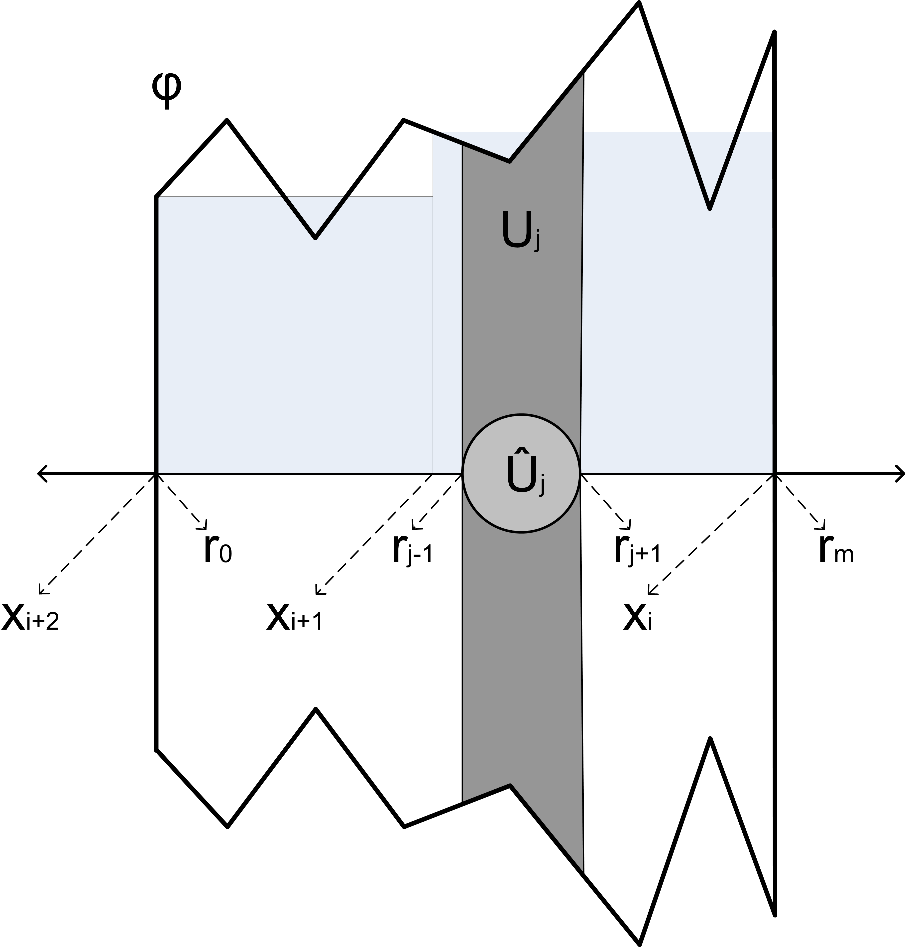
Figure 2. A more general $\varphi$ and the star-shaped domain $U_{j}$

To simplify the notation we introduce $M:=\varphi(x_{i+1})/2K_{2}K_{1}$. Thus,

$$|sy+(1-s)\tilde{y}| < s\frac{M}{4K_{1}}+(1-s)\varphi(\tilde{x})\leq s\left(\frac{M}{4}-M\right)+\varphi(\tilde{x})$$

$$\leq -\frac{3}{4}sM+\left(\varphi(\tilde{x})-\varphi(sx+(1-s)\tilde{x})\right)+\varphi(sx+(1-s)\tilde{x})$$

$$\leq -\frac{3}{4}sM+K_{1}s|\tilde{x}-x|+\varphi(sx+(1-s)\tilde{x})$$

$$\leq -\frac{3}{4}sM+K_{1}s\frac{M}{2K_{1}}+\varphi(sx+(1-s)\tilde{x})<\varphi(sx+(1-s)\tilde{x}).$$

Now, using (5.22) and (5.23), it can be seen that the diameter of $U_{j}$ and the radius of $\hat{U}_{j}$ are comparable to $\varphi(x_{i+1})$. Thus, using estimate (5.20), we can conclude that $M_{2}$ in (e) can be taken as a constant just depending on $K_{1}$, $K_{2}$, $n$ and $p$. ∎

6. Divergence problem and Stokes equations on Hölder domains

In this section, we show the existence of a right inverse of the divergence operator and the well-posedness of the Stokes equations on an arbitrary bounded Hölder-$\alpha$ domain $\Omega$, i.e. the boundary of $\Omega$ is locally the graph of a function that verifies $|\varphi(x)-\varphi(x^{\prime})|\leq K_{\varphi}|x-x^{\prime}|^{\alpha}$, for all $x,x^{\prime}$. Thus, we start this section studying a domain in ${\mathbb{R}}^{n}$ defined by the graph of a positive Hölder-$\alpha$ function $\varphi:(\frac{-3l}{2},\frac{3l}{2})^{n-1}\to{\mathbb{R}}$, where $0<\alpha\leq 1$ and $l>0$,

$$\Omega_{\varphi}:=\left\{(x,y)\in(-l/2,l/2)^{n-1}\times{\mathbb{R}}\,:\,0<y<\varphi(x)\right\}\subset{\mathbb{R}}^{n}.$$ (6.24)

In addition, we assume that $\varphi\geq 2l$ but $\varphi\not\geq 3l$, and $l\leq 1$. Now, $\Omega$ is locally as $\Omega_{\varphi}$, however the distance to the boundary of $\Omega$ is not necessarily equivalent to the distance to the graph of $\varphi$ defined over $(-l/2,l/2)^{n-1}$. Thus, in order to solve this problem, we assume that $\Omega$ is locally an expanded version of $\Omega_{\varphi}$:

$$\Omega_{\varphi,E}:=\{(x,y)\in(-3l/2,3l/2)^{n-1}\times{\mathbb{R}}\,:\,y<\varphi(x)\}\subset{\mathbb{R}}^{n}.$$ (6.25)

With this new approach of the problem, the distance to $\partial\Omega$ is equivalent to the distance to $G$ over $\Omega_{\varphi}$, where

$$G:=\{(x,y)\in(-5l/2,5l/2)^{n-1}\times{\mathbb{R}}\,:\,y=\varphi(x)\}.$$ (6.26)

Let us denote the distance to $G$ as $d_{G}$.

Lemma 6.1.

Let $\Omega_{\varphi}$ be the domains defined on (6.24), $1<p<\infty$, and $\kappa\geq 0$. Given $f\in L^{p}(\Omega_{\varphi},d_{G}^{-\kappa})$ with vanishing mean value, there exists a vector field ${\bf u}\in W^{1,p}_{0}(\Omega_{\varphi},d_{G}^{1-\alpha-\kappa})^{n}$ solution of $\mbox{div\,}{\bf u}=f$ such that

$$\|D{\bf u}\|_{L^{p}(\Omega_{\varphi},d_{G}^{1-\alpha-\kappa})}\leq C\|f\|_{L^{p}(\Omega_{\varphi},d_{G}^{-\kappa})},$$

where $C$ depends only on $K_{\varphi}$, $\alpha$, $n$, $p$ and $\kappa$.

Proof.

We start defining a collection of cubes in the style of the Whitney cubes, but in this case the diameter of the cubes is comparable to $d_{G}$ instead of the distance to $\partial\Omega_{\varphi}$. The construction of this collection of open cubes $\{Q_{t}\}_{t\in\Gamma}$ consists on piling cubes as boxes one over the other one in such a way that the common length of the sides of each cube is comparable to $d_{G}$. The cubes are constructed level by level starting by level 0, which has just the cube $Q_{a}=(\frac{-l}{2},\frac{l}{2})^{n-1}\times(0,l)$. The construction of the cubes induces the tree structure of the index set $\Gamma$ where the parents of the index of the cubes in level $m+1$ are the index of the cubes in level $m$. Thus, suppose that we have defined all the cubes in level $m$, and let $Q_{t}=Q_{t}^{\prime}\times(y_{t,1},y_{t,2})$ be one of them. Let us denote by $l_{t}$ the common length of the sides of $Q_{t}$. Thus, all the cubes $Q_{s}$’s in level $m+1$ with $s_{p}=t$ are defined in the following way: we move up and then expand $Q_{t}$ to obtain $Q=3(Q_{t}+(0,\cdots,0,l_{t}))$ thus

1. if $Q\subset\Omega_{\varphi,E}$ there is just one cube $Q_{s}$ on level $m+1$ such that $s_{p}=t$ and it is $Q_{s}=Q_{t}+(0,\cdots,0,l_{t})$,

2. if $Q\not\subset\Omega_{\varphi,E}$ there are $2^{n-1}$ cubes $Q_{s}$ with $s_{p}=t$ and they are written as $Q_{s}=Q^{\prime}_{t,1/2}\times(y_{t,2},y_{t,2}+l_{t}/2)$, where $Q^{\prime}_{t,1/2}$ is one of cubes in ${\mathbb{R}}^{n-1}$ obtained by splitting $Q_{t}^{\prime}$ into $2^{n-1}$ cubes with length of its sides equal to $l_{t}/2$.

See figure 3 for an example of the construction.

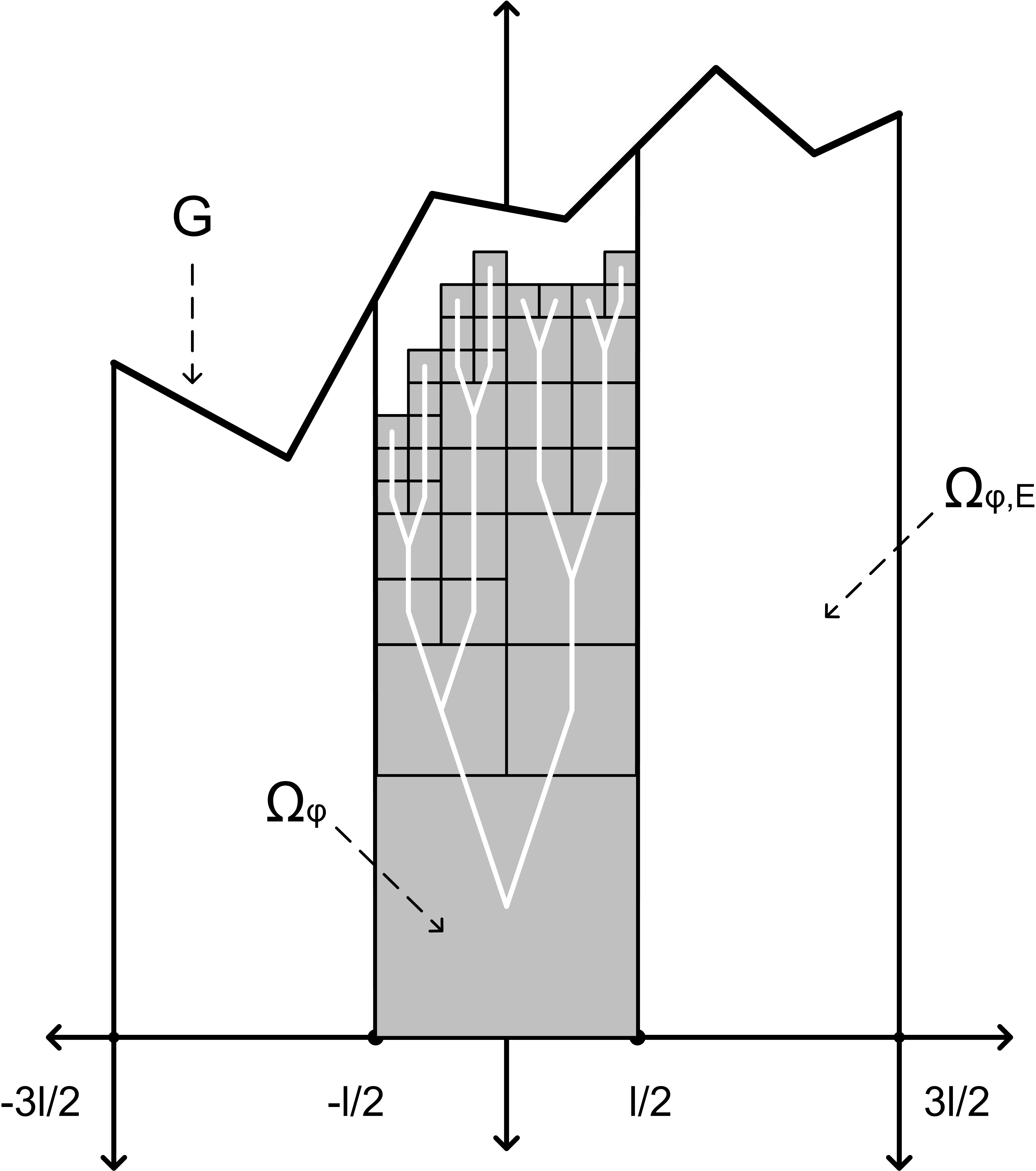
Figure 3. Under the graph of a Hölder-$\alpha$ function

Note that the common length of the sides of the cubes $\{Q_{t}\}_{t\in\Gamma}$ decreases with respect to the order $\succeq$ inherited from the tree. Indeed,

$$l_{t}\leq l_{s}\hskip 56.9055pt\text{ if }t\succeq s.$$ (6.27)

Let us show another property satisfied by this collection. Given $Q_{t}$, it satisfies

$$l_{t}\leq dist(Q_{t},G)\leq C_{n}\,l_{t}.$$ (6.28)

The first inequality follows from the definition. To prove the second one, note that there exists $Q_{s}$ with $s\preceq t$ and $l_{s}=2l_{t}$ such that $3(Q_{s}+(0,\cdots,0,l_{s}))\not\subset\Omega_{\varphi,E}$. Thus, following the notation $Q_{s}=Q_{s}^{\prime}\times(y_{s,1},y_{s,2})$ and $Q_{t}=Q_{t}^{\prime}\times(y_{t,1},y_{t,2})$, we can assert that there exists $x_{s}\in 3Q_{s}^{\prime}$ such that $\varphi(x_{s})<y_{s,2}+2l_{s}\leq y_{t,1}+4l_{t}.$

On the other hand, $\varphi\geq y_{t,1}+2l_{t}$ in $Q_{t}^{\prime}$, and $Q_{t}^{\prime}\subseteq Q^{\prime}_{s}$. Thus, using the convexity of $3Q^{\prime}_{s}$ and the continuity of $\varphi$, there is another point in $3Q_{s}^{\prime}$, let us represent it with the same notation $x_{s}$, such that

$$y_{t,1}+2l_{t}\leq\varphi(x_{s})\leq y_{t,1}+4l_{t}.$$ (6.29)

Observe that any point in $Q^{\prime}_{t}$ has a distance to $x_{s}$ lesser than the diameter of $3Q^{\prime}_{s}$, which equals $6\sqrt{n-1}\,l_{t}$. Thus,

$$dist(Q_{t},G)\leq dist(Q_{t},(x_{s},\varphi(x_{s})))\leq\sqrt{diam(3Q^{\prime}_{s})^{2}+(3l_{t})^{2}}\leq 3\sqrt{4n-3}\,l_{t}.$$

Now, we are ready to define the collection $\{\Omega_{t}\}_{t\in\Gamma}$ of subdomains of $\Omega_{\varphi}$ to apply Theorem 3.2. The first subdomain $\Omega_{a}$ is the cube $Q_{a}$, and the other ones are the $n$ dimensional rectangles defined by

$$\Omega_{t}:=Q^{\prime}_{t}\times(y_{t,1}-\frac{1}{2}l_{t},y_{t,2}),$$ (6.30)

where $Q_{t}=Q_{t}^{\prime}\times(y_{t,1},y_{t,2})$. Observe that $y_{t,2}=y_{t,1}+l_{t}$.

It can be seen that conditions (a) and (c) are valid, with a constant $N=2$. Indeed, $\Omega_{t}\cap\Omega_{s}\neq\emptyset$ for $t\neq s$ if and only if one index is the parent of the other one.

Next, if we define the collection $\{B_{t}\}_{t\neq a}$ as

$$B_{t}:=\Omega_{t}\cap\Omega_{t_{p}}=Q^{\prime}_{t}\times(y_{t,1}-\frac{1}{2}l_{t},y_{t,1}),$$

(b) follows.

Now, let us show that (d) is verified with $\bar{\omega}:=d_{G}^{1-\alpha}$. In order to estimate $\omega$, we take the point $x_{s}\in{\mathbb{R}}^{n-1}$ that verifies (6.29). Then , for all $x_{t}\in Q^{\prime}_{t}$ it follows that

$$|\varphi(x_{t})|\leq|\varphi(x_{t})-\varphi(x_{s})|+|\varphi(x_{s})|\leq C_{n,\alpha}K_{\varphi}l_{t}^{\alpha}+4l_{t}+y_{t,1}.$$

Thus, $|W_{t}|\leq C_{n,\alpha}(K_{\varphi}+l_{t}^{1-\alpha})l_{t}^{n-1+\alpha}$ and $|B_{t}|=\frac{1}{2}l^{n}_{t}$. Then, given $s\in\Gamma$ with $s_{p}=t$, we have that $|W_{s}|\leq|W_{t}|$ and $|B_{s}|\geq 2^{-n}|B_{t}|$. Thus,

$$\omega(x,y)\geq\dfrac{C_{n,\alpha}}{(K_{\varphi}+l^{n-1+\alpha})}l_{t}^{1-\alpha}=\dfrac{C_{n,\alpha}}{(K_{\varphi}+l^{n-1+\alpha})}d_{G}^{1-\alpha},$$

if $(x,y)$ belong to $\Omega_{t}$. Then,

$$\mathop{\mathrm{ess\,inf}}_{(x,y)\in\Omega_{t}}\omega(x,y)\geq\dfrac{C_{n,\alpha}}{(K_{\varphi}+l^{n-1+\alpha})}l_{t}^{1-\alpha}\geq\mathop{\mathrm{ess\,sup}}_{(x,y)\in\Omega_{t}}\dfrac{C_{n,\alpha}}{(K_{\varphi}+l^{n-1+\alpha})}d_{G}^{1-\alpha}(x,y),$$

proving (d) with a constant $M_{1}$ depending only on $K_{\varphi}$, $n$, $\alpha$ and $l$.

In order to study (e) we take $\hat{\omega}:=d_{G}^{-\kappa}$. Using that $\kappa\geq 0$ and $d_{G}$ is bounded over $\Omega_{\varphi}$, it follows that $L^{p}(\Omega_{\varphi},d_{G}^{-\kappa})\subset L^{1}(\Omega_{\varphi})$. Next, from (6.28) we have that $\frac{1}{2}l_{t}\leq dist(\Omega_{t},G)\leq C_{n}\,l_{t}$, hence we can assume that $d_{G}^{1-\alpha}$ is constant over $\Omega_{t}$ reducing the problem to the case $\kappa=0$. Now, $\Omega_{t}$, with $t\neq a$, is a translate of $(0,l_{t})^{n-1}\times(0,3l_{t}/2)$, thus, using Lemma 2.1, we can assert that $\Omega_{t}$ satisfies $\mbox{(div)}_{p}$ with a constant depending only on $n$.

Finally, the condition (f) follows from (6.27) and Lemma 3.1. Moreover, it can be observed that $d_{G}\leq C_{n}l_{s}$ in $\Omega_{s}$ and $l_{s}\leq l_{t}$ if $s\succeq t$, hence $d_{G}\leq C_{n}l_{t}$ over $W_{t}$.

Now, given $g\in L^{p}(\Omega_{\varphi},d_{G}^{-\kappa})$ the function $gd_{G}^{-\kappa}$ belongs to $L^{p}(\Omega_{\varphi})$, and using Lemma 3.1, we have

$$\int_{\Omega}|Tg|^{p}d_{G}^{-p\kappa} = \sum_{t\neq a}\int_{B_{t}}d_{G}^{-p\kappa}\left(\dfrac{1}{|W_{t}|}\int_{W_{t}}|g|d_{G}^{-\kappa}d_{G}^{\kappa}\right)^{p}$$

$$\leq C_{n,p,\kappa}\sum_{t\neq a}\int_{B_{t}}d_{G}^{-p\kappa}l_{t}^{p\kappa}\left(\dfrac{1}{|W_{t}|}\int_{W_{t}}|g|d_{G}^{-\kappa}\right)^{p}$$

$$= C_{n,p,\kappa}\sum_{t\neq a}\int_{B_{t}}\left(\dfrac{1}{|W_{t}|}\int_{W_{t}}|g|d_{G}^{-\kappa}\right)^{p}\leq c_{n,p,\kappa}\|gd_{G}^{-\kappa}\|_{L^{p}(\Omega_{\varphi})},$$

proving the lemma. ∎

Theorem 6.1 (Divergence on Hölder-$\alpha$ domains).

Let $\Omega\subset{\mathbb{R}}^{n}$ be a bounded Hölder-$\alpha$ domain, and $1<p<\infty$. Given $f\in L^{p}_{0}(\Omega,d^{-\kappa})$, with $d$ the distance to $\partial\Omega$ and $\kappa\geq 0$, there exists a vector field ${\bf u}\in W^{1,p}_{0}(\Omega,d^{1-\alpha-\kappa})^{n}$ solution of $\mbox{div\,}{\bf u}=f$ with estimate

$$\|D{\bf u}\|_{L^{p}(\Omega,d^{1-\alpha-\kappa})}\leq C\|f\|_{L^{p}(\Omega,d^{-\kappa})},$$

where $C$ does not depend on $f$.

Proof.

$\Omega$ is a Hölder-$\alpha$ domain, thus $\partial\Omega$ is locally the graph of a Hölder-$\alpha$ function, after taking a rigid movement. In fact, we can assume that $\partial\Omega$ can be covered by a finite collection of open sets $\{U_{i}\}_{1\leq i\leq m}$ such that $\Omega_{i}:=U_{i}\cap\Omega$ is in the form (6.24), where the extended domain in (6.25) is the intersection of another open set $V_{i}\supset U_{i}$ with $\Omega$. The reason to consider these $V_{i}^{\prime}$s is just to have $d$ locally comparable to $d_{G}$. Also, it can be assumed that the finite collection $\{\Omega_{i}\}$ is minimal in the sense that for each $1\leq i\leq m$ the set $\Omega_{i}\setminus\bigcup_{j\neq i}U_{j}$ has a positive Lebesgue measure. Now, let us take a Lipschitz domain $\Omega_{0}\subset\subset\Omega$ such that $B_{i}:=(\Omega_{i}\cap U_{0})\setminus\bigcup_{j\neq i}U_{j}$ has a positive Lebesgue measure and $\cup_{i=0}^{m}\Omega_{i}=\Omega$.

Let us define the finite collection $\{\Omega_{i}\}_{0\leq i\leq m}$. The tree structure of the index set $\Gamma=\{0,1,\cdots,m\}$ is defined in such a way that two nodes $i$ and $j$ are connected by an edge if and only if one of those is the root $a=0$. Thus, the partial order is given by $i\preceq j$ if and only if $i=0$.

The proof of this theorem follows the idea used to prove Theorem 3.2 with a minor difference in condition (e). In this case, the condition has two different weights and it can be stated as: given $g\in L^{p}(\Omega_{t},d^{-\kappa})$ with vanishing mean value there is a solution ${\bf v}\in W_{0}^{p}(\Omega_{t},d^{1-\alpha-\kappa})^{n}$ of $\mbox{div\,}{\bf v}=g$ with

$$\|D{\bf v}\|_{L^{p}(\Omega_{t},d^{-\kappa})}\leq M_{2}\|g\|_{L^{p}(\Omega_{t},d^{1-\alpha-\kappa})}$$

for all $t\in\Gamma$, where the positive constant $M_{2}$ does not depend on $t$. This condition was proved in Lemma 6.1.

Now, note that $\omega$ takes finite different positive values, thus the weight $\bar{\omega}$ can be assumed constant over $\Omega$ obtaining (d). On the other hand, the operator $T$ has its support in $\Omega_{0}$, which is compactly contained in $\Omega$. Thus, the weight $\hat{\omega}:=d^{1-\alpha-\kappa}$ can be assumed constant. Hence, from 3.1, the operator $T:L^{p}(\Omega,d^{1-\alpha-\kappa})\to L^{p}(\Omega,d^{1-\alpha-\kappa})$ is continuous and (f) is satisfied.

It can be noted that condition (a), (b) and (c) can be easily verified from the definition of the collection of subdomains and it finiteness. Thus, the proof goes as in Theorem 3.2. ∎

In the last theorem we show the well-posedness of the Stokes equations on bounded Hölder-$\alpha$ domains.

Theorem 6.2 (Stokes on Hölder-$\alpha$ domains).

Given $\Omega\subset{\mathbb{R}}^{n}$ a bounded Hölder-$\alpha$ domain, and two functions $h\in L_{0}^{2}(\Omega,d^{\alpha-1})$, and ${\bf g}\in H^{-1}(\Omega)^{n}$. Then, there exists a unique solution $({\bf u},p)\in H_{0}^{1}(\Omega)^{n}\times L^{2}(\Omega,d^{1-\alpha})$ of (2.2) with $\int_{\Omega}pd^{2(1-\alpha)}=0$. Moreover,

$$\|D{\bf u}\|_{L^{2}(\Omega)}+\|p\|_{L^{2}(\Omega,d^{1-\alpha})}\leq C\left(\|{\bf g}\|_{H^{-1}(\Omega)}+\|h\|_{L^{2}(\Omega,d^{\alpha-1})}\right),$$ (6.31)

where $d$ is the distance to $\partial\Omega$, and $C$ depends only on $\Omega$.

Proof.

The proof of this theorem follows the same idea as the proof of Theorem 5.2. ∎

References

- [1] G. Acosta, R. Durán, and A. Lombardi, Weighted Poincaré and Korn inequalities for Hölder domains, Math. Meth. Appl. Sci. (MMAS) 29(4) (2006), pp. 387-400.
- [2] G. Acosta, R. Durán, and F. López García, Korn inequality and divergence operator: counterexamples and optimality of weighted estimates, Proc. of the AMS., 141 (2013), pp. 217-232.
- [3] G. Acosta, R. G. Durán, and M. A. Muschietti, Solutions of the divergence operator on John Domains, Advances in Mathematics 206(2) (2006), pp. 373-401.
- [4] D. N. Arnold, L. R. Scott, and M. Vogelius, Regular inversion of the divergence operator with Dirichlet boundary conditions on a polygon, Ann. Scuola Norm. Sup. Pisa Cl. Sci. (4) 15(2) (1988), pp. 169-192.
- [5] M. E. Bogovskii, Solution of the first boundary value problem for the equation of continuity of an incompressible medium, Soviet Math. Dokl. 20 (1979), pp. 1094-1098.
- [6] L. Diening, M. Ružička, and K. Schumacher, A decomposition technique for John domains, Ann. Acad. Sci. Fenn. Math. 35 (2010), pp. 87-114.
- [7] J. Duoandikoetxea, Fourier analysis, American Mathematical Society, Providence, RI, 2001.
- [8] R. Durán, and F. López García, Solutions of the divergence and analysis of the Stokes equations in planar domains, Math. Mod. Meth. Appl. Sci. 20(1) (2010), pp. 95-120.
- [9] R. Durán, and F. López García, Solutions of the divergence and Korn inequalities on domains with an external cusp, Ann. Acad. Sci. Fenn. Math. 35(2) (2010), pp. 421-438.
- [10] R. G. Durán, M. A. Muschietti, E. Russ, and P. Tchamitchian, Divergence operator and Poincaré inequalities on arbitrary bounded domains, Complex Var. Elliptic Equ. 55(8-10) (2010), pp. 795-816.
- [11] R. G. Durán, and M. A. Muschietti, An explicit right inverse of the divergence operator which is continuous in weighted norms, Studia Math. 148(3) (2001), pp. 207-219.
- [12] K. O. Friedrichs, On the boundary value problem of the theory of elasticity and Korn’s inequality, Ann. of Math. 48(2) (1947), pp. 441-471.
- [13] G. P. Galdi, An introduction to the mathematical theory of the Navier-Stokes equations, Springer Monographs in Mathematics, Springer, New York, 2011.
- [14] O. A. Ladyzhenskaya, The mathematical theory of viscous incompressible flow, Gordon and Breach, New York-London-Paris, 1969.
- [15] K. Schumacher, Solutions to the equation in weighted Sobolev spaces, Technical Report 2511, FB Mathematik, TU Darmstadt, 2007.
- [16] E. M. Stein, Singular integrals and differentiability properties of functions, Princeton Mathematical Series, No. 30 Princeton University Press, Princeton, N.J. 1970.