Observational signatures of anisotropic inflationary models

Abstract

We study observational signatures of two classes of anisotropic inflationary models in which an inflaton field couples to (i) a vector kinetic term $F_{\mu\nu}F^{\mu\nu}$ and (ii) a two-form kinetic term $H_{\mu\nu\lambda}H^{\mu\nu\lambda}$. We compute the corrections from the anisotropic sources to the power spectrum of gravitational waves as well as the two-point cross correlation between scalar and tensor perturbations. The signs of the anisotropic parameter $g_{*}$ are different depending on the vector and the two-form models, but the statistical anisotropies generally lead to a suppressed tensor-to-scalar ratio $r$ and a smaller scalar spectral index $n_{s}$ in both models. In the light of the recent Planck bounds of $n_{s}$ and $r$, we place observational constraints on several different inflaton potentials such as those in chaotic and natural inflation in the presence of anisotropic interactions. In the two-form model we also find that there is no cross correlation between scalar and tensor perturbations, while in the vector model the cross correlation does not vanish. The non-linear estimator $f_{\rm NL}$ of scalar non-Gaussianities in the two-form model is generally smaller than that in the vector model for the same orders of $|g_{*}|$, so that the former is easier to be compatible with observational bounds of non-Gaussianities than the latter.

I Introduction

The measurements of Cosmic Microwave Background (CMB) temperature anisotropies and large-scale structures have significantly improved in accuracy over the last decade WMAP1 ; WMAP9 ; Rei ; Atacama ; LSS1 ; LSS2 . In particular, the recently released Planck data Adecosmo ; Adeinf ; Adenon showed that the primordial power spectrum of curvature perturbations is slightly red-tilted from the exact scale-invariance. This is consistent with the theoretical prediction of standard slow-roll inflation driven by a nearly flat potential of a scalar field $\phi$ (called “inflaton”) oldper .

While the WMAP and Planck data support the inflationary scenario overall, there are some anomalies in the data WMAP9 ; Adecosmo which are difficult to be addressed in the context of single-field slow-roll inflation. One of them is broken rotational invariance of the CMB perturbations aniobser1 ; aniobser2 ; aniobser3 . The power spectrum of curvature perturbations $\zeta$ with broken statistical isotropy can be expressed in the form Carroll

$${\cal P}_{\zeta}({\bm{k}})={\cal P}_{\zeta}^{(0)}(k)\,\left(1+g_{*}\cos^{2}\theta_{{\bm{k}},{\bm{V}}}\right)\,,$$ (1)

where ${\bm{k}}$ is the comoving wave number, ${\cal P}_{\zeta}^{(0)}(k)$ is the isotropic power spectrum, $g_{*}$ characterizes the deviation from the isotropy, ${\bm{V}}$ is a privileged direction close to the ecliptic poles, and $\theta_{{\bm{k}},{\bm{V}}}$ is the angle between ${\bm{k}}$ and ${\bm{V}}$. From the WMAP data, Groeneboom et al. aniobser3 obtained the bound $g_{*}=0.29\pm 0.031$ with the exclusion of $g_{*}=0$ at $9\sigma$ by including the CMB multipoles up to $\ell=400$. There is still a possibility that some systematic effect such as the asymmetry of the instrument beam accounts for broken rotational invariance Hanson .

If broken statistical isotropy is really present for primordial perturbations, we need to go beyond the slow-roll single-field inflationary scenario to explain the origin of statistical anisotropies review1 ; review2 . For the models in which the inflaton $\phi$ has a coupling with a vector kinetic term $F_{\mu\nu}F^{\mu\nu}$, there exists an attractor-like solution along which an anisotropic vector hair survives even during inflation Watanabe (see Refs. early for early related works and Refs. powerlaw ; anipapers for rich phenomenologies of anisotropic inflation). Even if the background energy density of the vector field is suppressed relative to that of the inflaton, the isotropic power spectrum ${\cal P}_{\zeta}^{(0)}(k)$ is modified to have the form (1) with a negative anisotropic parameter $g_{*}$ Gum ; Watanabe:2010fh ; Bartolo . Moreover the non-linear estimator $f_{\rm NL}$ of scalar non-Gaussianities can be as large as the order of 10 for the squeezed shape averaged over all directions of a wave number ${\bm{k}}_{3}$ with ${\bm{k}}_{1}\simeq-{\bm{k}}_{2}$ Bartolo ; Shiraishi (see also Refs. Barnaby for the large non-Gaussianities generated by vector fields).

Recently, the present authors showed that anisotropic inflation can be also realized for the model in which the inflaton couples to a two-form field with the kinetic term $H_{\mu\nu\lambda}H^{\mu\nu\lambda}$ Ohashi (see Ref. Watanabe:2010fh for an early proposal). In this case, the anisotropic power spectrum is given by Eq. (1) with $g_{*}>0$. Since the sign of $g_{*}$ is opposite to that in the vector model, we can observationally distinguish between the two anisotropic inflationary scenarios. In Ref. Ohashi the bispectrum and trispectrum of curvature perturbations have been also evaluated in the two-form model by using the interacting Hamiltonian picture Maldacena:2002vr ; Bartolo . It was shown that, in the strict squeezed limit, the non-linear estimator $f_{\rm NL}$ vanishes and that, in the equilateral and enfolded limits, $f_{\rm NL}$ can be larger than the order of 10.

In this paper we place observational constraints on two anisotropic inflation models based on the vector and the two-form fields in the light of the recent Planck data Adecosmo ; Adeinf ; Adenon . We first derive the anisotropic power spectra of gravitational waves to evaluate the tensor-to-scalar ratio $r$ correctly. Using the observational bounds of $r$ as well as the scalar spectral index $n_{s}$ constrained by the joint data analysis of Planck and other measurements Adeinf ; Kuro , we test for several representative models such as chaotic and natural inflation in the presence of anisotropic corrections to the scalar and tensor power spectra.

We also compute the cross correlations between curvature perturbations and gravitational waves. While the cross correlation survives in the vector model, it vanishes in the two-form model. This property is useful to distinguish between the two anisotropic inflationary scenarios from the correlation between the observed temperature perturbation and the B-mode polarization (TB correlation) Watanabe2 .

We also revisit the estimation of the anisotropic scalar non-Gaussianities for several different shapes of momentum dependence (local, equilateral, and enfolded shapes) in both the vector and the two-form models. In fact, we show that the local non-linear estimators in the strict squeezed limit (${\bm{k}}_{3}\to 0$ with $\theta_{{\bm{k}}_{1},{\bm{k}}_{3}}\to\pi/2$, $\theta_{{\bm{k}}_{2},{\bm{k}}_{3}}\to\pi/2$) vanish in both models. However, if we average over all directions of a wave number ${\bm{k}}_{3}$ with ${\bm{k}}_{1}\simeq-{\bm{k}}_{2}$ for nearly squeezed shapes Bartolo , we have non-zero values of $f_{\rm NL}$ for $|g_{*}|>0$. Taking this prescription, we show that the local non-linear estimator $f_{\rm NL}^{\rm local}$ in the two-form model is smaller than that in the vector model by one order of magnitude for the same order of $|g_{*}|$.

This paper is organized as follows. In Sec. II we review the background dynamics of anisotropic inflation for both the vector and the two-form models. In Sec. III we derive anisotropic corrections to the scalar/tensor power spectra and also evaluate the cross correlation between curvature perturbations and gravitational waves. In Sec. IV we put constraints on several different inflaton potentials by using the 68 % CL and 95 % CL observational contours in the $(n_{s},r)$ plane. In Sec. V we compare two anisotropic inflationary models from the non-linear estimator $f_{\rm NL}$ of scalar non-Gaussianities. Sec. VI is devoted to conclusions.

II inflation with anisotropy

In this section we briefly review the background dynamics of anisotropic inflation for two classes of models in which the inflaton field $\phi$ couples to (i) a vector field $A_{\mu}$ Watanabe and (ii) a two-form field $B_{\mu\nu}$ Ohashi . For suitable choices of couplings, the energy densities of the fields $A_{\mu}$ and $B_{\mu\nu}$ can survive even during inflation. For details, we refer the reader to the review articles review1 ; review2 .

II.1 $f(\phi)^{2}F_{\mu\nu}F^{\mu\nu}$ model

Let us first discuss the vector model given by the action

$$S = \int d^{4}x\sqrt{-g}\left[\frac{M_{\rm pl}^{2}}{2}R-\frac{1}{2}\partial_{\mu}\phi\partial^{\mu}\phi-V(\phi)-\frac{1}{4}f(\phi)^{2}F_{\mu\nu}F^{\mu\nu}\right]\,,$$ (2)

where $g$ is the determinant of the metric $g_{\mu\nu}$, $M_{\rm pl}$ is the reduced Planck mass, and $R$ is the scalar curvature. $V(\phi)$ and $f(\phi)$ are a potential and a kinetic function of the inflaton $\phi$, respectively. The field strength of the vector field is characterized by

$$F_{\mu\nu}=\partial_{\mu}A_{\nu}-\partial_{\nu}A_{\mu}\ .$$ (3)

Now, we consider cosmological solutions in this system. Without loosing the generality, one can take $x$-axis for the direction of the vector field. Using the gauge invariance, we can express the vector field as

$$A_{\mu}dx^{\mu}=v(t)dx\,,$$ (4)

where $v(t)$ is a function of the cosmic time $t$. Even if initial inhomogeneities and isotropies in $v$ are present, it was shown that only the background field $v(t)$ survives during anisotropic inflation in the Bianchi type I Universe Watanabe:2010fh . The same conclusion also applies to more general anisotropic backgrounds Hervik . There remains the rotational symmetry in the $(y,z)$ plane. Hence, we can take the metric ansatz

$$ds^{2}=-dt^{2}+e^{2\alpha(t)}\left[e^{-4\sigma(t)}dx^{2}+e^{2\sigma(t)}(dy^{2}+dz^{2})\right]\ ,$$ (5)

where $e^{\alpha}\equiv a$ and $\sigma$ are the isotropic scale factor and the spatial shear, respectively. It is easy to solve the equation of motion for $v$ as

$$\dot{v}=p_{A}\,f(\phi)^{-2}e^{-\alpha-4\sigma}\,,$$ (6)

where $p_{A}$ is a constant of integration and an overdot denotes a derivative with respect to the cosmic time $t$.

The Friedmann equation and the inflaton equation of motion are given, respectively, by

$$H^{2} = \dot{\sigma}^{2}+\frac{1}{3M_{\rm pl}^{2}}\left[\frac{1}{2}\dot{\phi}^{2}+V(\phi)+\frac{p_{A}^{2}}{2}f(\phi)^{-2}e^{-4\alpha-4\sigma}\right]\,,$$ (7)

$$\ddot{\phi} = -3\dot{\alpha}\dot{\phi}-V_{,\phi}+p_{A}^{2}f(\phi)^{-3}f_{,\phi}e^{-4\alpha-4\sigma}\,,$$ (8)

where $H\equiv\dot{\alpha}$ is the Hubble expansion rate, and $V_{,\phi}\equiv dV/d\phi$, $f_{,\phi}\equiv df/d\phi$. We define the energy density of the vector field as

$$\rho_{A}\equiv\frac{p_{A}^{2}}{2}f(\phi)^{-2}e^{-4\alpha-4\sigma}\,.$$ (9)

In order to sustain inflation, the potential energy $V(\phi)$ of the inflaton needs to dominate over $\dot{\phi}^{2}/2$ and $\rho_{A}$. Since the shear term $\Sigma\equiv\dot{\sigma}$ should be suppressed relative to $H$, the Friedmann equation (7) reads

$$H^{2}=\dot{\alpha}^{2}\simeq\frac{V(\phi)}{3M_{\rm pl}^{2}}\,.$$ (10)

If $f$ is a rapidly decreasing function in time, it happens that $\rho_{A}$ does not decay. In particular, for the coupling

$$f(\phi)=e^{-2\alpha}=a^{-2}\,,$$ (11)

the energy density (9) stays nearly constant (under the approximation $|\sigma|\ll\alpha$). In this case, neglecting the contribution of the vector field on the r.h.s. of Eq. (8), the field $\phi$ satisfies the slow-roll equation of motion $3\dot{\alpha}\dot{\phi}\simeq-V_{,\phi}$. Combining this equation with Eq. (10), it follows that $d\alpha/d\phi\simeq-V/(M_{\rm pl}^{2}V_{,\phi})$. Then, the critical coupling (11) can be expressed as

$$f(\phi)=e^{2\int\frac{V}{M_{\rm pl}^{2}V_{,\phi}}d\phi}\,.$$ (12)

The shear term obeys the equation of motion

$$\dot{\Sigma}=-3H\Sigma+\frac{2\rho_{A}}{3M_{\rm pl}^{2}}\,.$$ (13)

If an anisotropy converges to a nearly constant value $\Sigma$, then the quantity $\Sigma/H$ reduces to

$$\frac{\Sigma}{H}\simeq\frac{2\rho_{A}}{3V}\,,$$ (14)

where we used Eq. (10). In the following, let us estimate the ratio $\Sigma/H$ during anisotropic inflation. Ignoring the $\ddot{\phi}$ term in Eq. (8) and combining it with Eq. (10), it follows that

$$\frac{d\phi}{d\alpha}\simeq-\frac{M_{\rm pl}^{2}V_{,\phi}}{V}+\frac{2p_{A}^{2}}{V_{,\phi}}e^{-4\alpha-4\sigma-4\int\frac{V}{M_{\rm pl}^{2}V_{,\phi}}d\phi}\,,$$ (15)

where we used Eq. (12). Neglecting the variation of $\phi/M_{\rm pl}$ relative to that of $\alpha$, we can integrate Eq. (15) to give

$$e^{4\alpha+4\sigma+4\int\frac{V}{M_{\rm pl}^{2}V_{,\phi}}d\phi}\simeq\frac{8p_{A}^{2}V}{M_{\rm pl}^{2}V_{,\phi}^{2}}(\alpha+\alpha_{0})\,,$$ (16)

where $\alpha_{0}>0$ is an integration constant. Substituting Eq. (16) into Eq. (9), we have

$$r_{A}\equiv\frac{\rho_{A}}{\epsilon V}\simeq\frac{1}{8(\alpha+\alpha_{0})}\,,$$ (17)

where $\epsilon\equiv-\dot{H}/H^{2}$, and we used the fact that $\epsilon\simeq(M_{\rm pl}^{2}/2)(V_{,\phi}/V)^{2}$ under the slow-roll approximation. Provided that $\alpha\ll\alpha_{0}$, the ratio $r_{A}$ is nearly constant. As we will see in Sec. III, the quantity $r_{A}$ is related to the anisotropic parameter $g_{*}$ appearing in the power spectrum of curvature perturbations. From Eqs. (14) and (17) we obtain

$$\frac{\Sigma}{H}\simeq\frac{1}{12(\alpha+\alpha_{0})}\epsilon\,,$$ (18)

which means that the anisotropy survives during inflation for $\alpha\ll\alpha_{0}$.

The above discussion can be generalized to the coupling of the form

$$f(\phi)=e^{2c\int\frac{V}{M_{\rm pl}^{2}V_{,\phi}}d\phi}\,,$$ (19)

where $c$ is a constant parameter. If the condition

$$c=\frac{M_{\rm pl}^{2}}{2}\frac{f_{,\phi}}{f}\frac{V_{,\phi}}{V}>1$$ (20)

is satisfied, the energy density of the vector field grows as $\rho_{A}\propto e^{4(c-1)\alpha}$ during the slow-roll phase of the inflaton. Eventually, the vector field becomes relevant to the inflaton dynamics governed by Eq. (8). However, when the third term on the r.h.s. of Eq. (8) dominates over the second term, the inflaton does not roll down, which makes $\rho_{A}$ decrease. Hence the condition $\rho_{A}\ll V(\phi)$ is always satisfied. In this way, there appears an attractor where inflation continues even when the vector field affects the inflaton dynamics. For the coupling (19) the shear to the Hubble expansion rate approaches the value Watanabe

$$\frac{\Sigma}{H}\simeq\frac{1}{3}\frac{c-1}{c}\epsilon\,.$$ (21)

Thus, inflation is slightly anisotropic and the energy density of the vector field never decays for the coupling (19) with $c>1$. From Eqs. (14) and (21) it follows that the ratio $r_{A}$ defined in Eq. (17) is nearly constant, i.e., $r_{A}\simeq(c-1)/(2c)$.

In the attractor regime where the vector field contributes to the dynamics of the system there is the relation $d\alpha/d\phi\simeq-cV/(M_{\rm pl}^{2}V_{,\phi})$ review2 , in which case the coupling (19) evolves as $f(\phi)\propto a^{-2}$, i.e., the same as Eq. (11). In Sec. III we shall use this property for the evaluation of two-point correlation functions of primordial perturbations.

II.2 $f(\phi)^{2}H_{\mu\nu\lambda}H^{\mu\nu\lambda}$ model

In the presence of a two-form field coupled to the inflaton Ohashi , anisotropic hair can survive during inflation as in the vector model. In this case, the action reads

$$S=\int d^{4}x\sqrt{-g}\left[\frac{M_{\rm pl}^{2}}{2}R-\frac{1}{2}\partial_{\mu}\phi\partial^{\mu}\phi-V(\phi)-\frac{1}{12}f(\phi)^{2}H_{\mu\nu\lambda}H^{\mu\nu\lambda}\right]\,,$$ (22)

where the field strength $H_{\mu\nu\lambda}$ is related to a two-form field $B_{\mu\nu}$, as

$$H_{\mu\nu\lambda}=\partial_{\mu}B_{\nu\lambda}+\partial_{\nu}B_{\lambda\mu}+\partial_{\lambda}B_{\mu\nu}\,.$$ (23)

Without loss of generality, one can take the $(y,z)$ plane in the direction of the two-form field. Then we can express $B_{\mu\nu}$ in the form

$$\frac{1}{2}B_{\mu\nu}\,dx^{\mu}\wedge dx^{\nu}=w(t)\,dy\wedge dz\,,$$ (24)

where $w(t)$ is a function with respect to $t$. Since there exists a rotational symmetry in the $(y,z)$ plane, the metric can be parametrized by the form (5). The equation of motion for the two-form field $w$ is easily solved as

$$\dot{w}=p_{B}\,f(\phi)^{-2}e^{\alpha+4\sigma}\,,$$ (25)

where $p_{B}$ is a constant of integration.

The Hubble parameter $H=\dot{\alpha}$ and the inflaton $\phi$ obeys the equations of motion

$$H^{2} = \dot{\sigma}^{2}+\frac{1}{3M_{\rm pl}^{2}}\left[\frac{1}{2}\dot{\phi}^{2}+V(\phi)+\frac{p_{B}^{2}}{2}f(\phi)^{-2}e^{-2\alpha+4\sigma}\right]\,,$$ (26)

$$\ddot{\phi} = -3\dot{\alpha}\dot{\phi}-V_{,\phi}+p_{B}^{2}f(\phi)^{-3}f_{,\phi}e^{-2\alpha+4\sigma}\,,$$ (27)

which are analogous to Eqs. (7) and (8) with the difference of the exponential factors. Defining the energy density of the two-form field as

$$\rho_{B}\equiv\frac{p_{B}^{2}}{2}f(\phi)^{-2}e^{-2\alpha+4\sigma}\,,$$ (28)

it follows that $\rho_{B}$ stays nearly constant for the coupling

$$f(\phi)=e^{-\alpha}=a^{-1}\,.$$ (29)

In the slow-roll regime of the inflaton there is the relation $d\alpha/d\phi\simeq-V/(M_{\rm pl}^{2}V_{,\phi})$, so that the coupling (29) can be expressed as

$$f(\phi)=e^{\int\frac{V}{M_{\rm pl}^{2}V_{,\phi}}d\phi}\,.$$ (30)

Since the shear $\Sigma=\dot{\sigma}$ satisfies the equation of motion

$$\dot{\Sigma}=-3H\Sigma-\frac{2\rho_{B}}{3M_{\rm pl}^{2}}\,,$$ (31)

the ratio $\Sigma/H$ should converge to

$$\frac{\Sigma}{H}=-\frac{2\rho_{B}}{3V}\,,$$ (32)

where Eq. (10) is used. The sign of $\Sigma/H$ is opposite to that of the vector model. During anisotropic inflation the ratio (32) reads Ohashi

$$\frac{\Sigma}{H}\simeq-\frac{1}{3(\alpha+\alpha_{0})}\epsilon\,,$$ (33)

where $\alpha_{0}>0$ is a constant. From Eqs. (32) and (33) we have

$$r_{B}\equiv\frac{\rho_{B}}{\epsilon V}\simeq\frac{1}{2(\alpha+\alpha_{0})}\,,$$ (34)

which is nearly constant for $\alpha\ll\alpha_{0}$. The ratio (34) appears in the anisotropic scalar power spectrum.

We can generalize the coupling (30) to the form

$$f(\phi)=e^{c\int\frac{V}{M_{\rm pl}^{2}V_{,\phi}}d\phi}\,,$$ (35)

where $c$ is a constant. For the super-critical case characterized by

$$c=M_{\rm pl}^{2}\frac{f_{,\phi}}{f}\frac{V_{,\phi}}{V}>1\,,$$ (36)

there is an attractor solution along which the ratio $\Sigma/H$ approaches the value Ohashi

$$\frac{\Sigma}{H}\simeq-\frac{2}{3}\frac{c-1}{c}\epsilon\,,$$ (37)

whose sign is opposite to Eq. (21). In this regime there is the relation $d\alpha/d\phi\simeq-cV/(M_{\rm pl}^{2}V_{,\phi})$, so that the coupling (35) evolves as Eq. (29). Note that the ratio $r_{B}$ is nearly constant, i.e., $r_{B}\simeq(c-1)/c$.

The anisotropy induced by the two-form field is the prolate-type, in contrast to the vector field which induces the oblate-type anisotropy. This difference comes from the fact the vector $A_{\mu}$ extending to the $x$-direction speeds down the expansion in that direction, while the two-form field $B_{\mu\nu}$ extending in the $(y,z)$ plane speeds down the expansion in the $(y,z)$-direction.

We note that the couplings (12) and (30), which give rise to anisotropic inflation, are present for any slow-roll inflaton potentials. For the exponential potential $V(\phi)=V_{0}e^{\lambda\phi/M_{\rm pl}}$ the couplings $f(\phi)$ are of the exponential forms $f(\phi)\propto e^{\mu\phi/M_{\rm pl}}$ powerlaw , as they often appear as a dilatonic coupling in string theory. For some inflaton potentials the functions $f(\phi)$ may not be so natural, but there is a possibility that such couplings can be motivated by future development of string theory or supergravity. It is worth mentioning that power-law kinetically driven anisotropic inflation (k-inflation kinf ) can be generally realized for the exponential couplings $f(\phi)\propto e^{\mu\phi/M_{\rm pl}}$ anikinf .

III Scalar and tensor power spectra and their correlations

In order to study observational signatures of anisotropic inflation, we need to know the two-point correlation functions of curvature perturbations and gravitational waves as well as their cross correlations. For the vector model the power spectrum of curvature perturbations was derived in Refs. Gum ; Watanabe:2010fh ; Bartolo , whereas the anisotropic contribution to gravitational waves in the same model was discussed in Refs. Gum ; Watanabe:2010fh . For the two-form field model the present authors obtained the anisotropic scalar power spectrum Ohashi , but the tensor power spectrum has not been derived yet. We also note that in the vector model the correlation between the temperature perturbation and the B-mode polarization was studied in Ref. Watanabe2 , but the cross-correlation between scalar and tensor perturbations in the two-form model has not been studied. Here we provide all the formulas of these observables convenient to confront with observations.

Since the anisotropy of the expansion rate needs to be sufficiently small for the compatibility with observations, it is a good approximation to neglect the effect of the anisotropic expansion for the derivation of the perturbation equations Watanabe:2010fh . The effect of the anisotropy appears in the interacting Hamiltonians between vector/two-form fields and scalar/tensor perturbations, by which the scalar/tensor power spectra are modified. Then, we consider a general perturbed metric with four scalar functions $A,B,\psi,E$ and the tensor perturbation $h_{ij}$ about the flat Friedmann-Lemaîtle-Robertson-Walker (FLRW) background Bardeen :

$$ds^{2}=a(\tau)^{2}\left\{-(1+2A)d\tau^{2}+2\partial_{i}Bd\tau dx^{i}+[(1+2\psi)\delta_{ij}+2\partial_{ij}E+h_{ij}]dx^{i}dx^{j}\right\}\,,$$ (38)

where $\tau=\int a^{-1}dt$ is the conformal time. After the end of inflation, the coupling $f(\phi)$ approaches a constant because the inflaton stabilizes at the potential minimum. In this case vector perturbations decay after inflation as in the standard scenario, so we neglect its contribution to the CMB observables relative to those of scalar and metric perturbations. We introduce the gauge-invariant comoving curvature perturbation Bardeen2 (see also Refs. zetadef ):

$$\zeta=\psi-\frac{H}{\dot{\phi}}\delta\phi\,,$$ (39)

where $\delta\phi$ is the perturbation of the inflaton $\phi$. In the following we choose the spatially flat gauge ($\psi=0$), in which case $\zeta=-(H/\dot{\phi})\delta\phi$. The curvature perturbation can be expressed in terms of the Fourier components with the comoving wave number ${\bm{k}}$, as

$$\zeta({\bm{x}},\tau)=\int\frac{d^{3}k}{(2\pi)^{3/2}}e^{i{\bm{k}}\cdot{\bm{x}}}\hat{\zeta}({\bm{k}},\tau)\,,\qquad\hat{\zeta}({\bm{k}},\tau)=\zeta(k,\tau)a({\bm{k}})+\zeta^{*}(k,\tau)a^{\dagger}(-{\bm{k}})\,,$$ (40)

where the annihilation and creation operators $a({\bm{k}})$ and $a^{\dagger}({\bm{k}^{\prime}})$ satisfy the commutation relation $[a({\bm{k}}),a^{\dagger}({\bm{k}^{\prime}})]=\delta^{(3)}({\bm{k}}-{\bm{k}}^{\prime})$. We define the scalar power spectrum ${\cal P}_{\zeta}$ in terms of the two-point correlation function of $\zeta$, as

$$\langle\hat{\zeta}({\bm{k}}_{1})\hat{\zeta}({\bm{k}}_{2})\rangle=\frac{2\pi^{2}}{k_{1}^{3}}\delta^{(3)}({\bm{k}}_{1}+{\bm{k}}_{2}){\cal P}_{\zeta}(k_{1})\,.$$ (41)

We decompose $\zeta$ into the isotropic field $\zeta^{(0)}$ and the contribution $\delta\zeta$ coming from the anisotropic fields, as

$$\zeta=\zeta^{(0)}+\delta\zeta\,.$$ (42)

In what follows we shall focus on the couplings (12) and (30), i.e., $c=1$. The situation is similar for the general couplings (19) and (35) with $c$ close to 1. Then we can employ the usual slow-roll relations $\dot{\phi}/H\simeq-M_{\rm pl}^{2}V_{,\phi}/V$ and $\epsilon=-\dot{H}/H^{2}\simeq(M_{\rm pl}^{2}/2)(V_{,\phi}/V)^{2}$, so that $\zeta^{(0)}\simeq\delta\phi/(M_{\rm pl}\sqrt{2\epsilon})$. The solution to the Fourier mode $\zeta^{(0)}(k,\tau)$, which recovers the Bunch-Davies vacuum state for the field perturbation $\delta\phi$ in the asymptotic past ($k\tau\to-\infty$), is given by Maldacena:2002vr

$$\zeta^{(0)}(k,\tau)=\frac{H(1+ik\tau)}{2\sqrt{\epsilon}M_{\rm pl}k^{3/2}}e^{-ik\tau}\,.$$ (43)

The power spectrum can be written as the sum of the two contributions from $\zeta^{(0)}$ and $\delta\zeta$, as ${\cal P}_{\zeta}={\cal P}^{(0)}_{\zeta}+\delta{\cal P}_{\zeta}$. Using the solution (43) long time after the Hubble radius crossing ($\tau\to 0$), the isotropic power spectrum of $\zeta$ is given by

$${\cal P}_{\zeta}^{(0)}=\frac{H^{2}}{8\pi^{2}\epsilon M_{\rm pl}^{2}}\,.$$ (44)

In Secs. III.1 and III.2 we shall evaluate the anisotropic corrections to ${\cal P}_{\zeta}^{(0)}$ in both the vector and the two-form field models.

For the tensor perturbation $h_{ij}$ we impose the traceless and transverse conditions $h_{ii}=h_{ij,j}=0$, as usual. The second-order action for $h_{ij}$ reads

$$S_{h}=\frac{M_{\rm pl}^{2}}{4}\int d\tau d^{3}x\,a^{2}\left[\frac{1}{2}h^{\prime}_{ij}h^{\prime}_{ij}-\frac{1}{2}h_{ij,k}h_{ij,k}\right]\,,$$ (45)

where the prime denotes the differentiation with respect to $\tau$. We have two physical degrees of freedom for $h_{ij}$ which can be characterized by the symmetric polarization tensors $e^{(+,\times)}_{ij}(\bm{k})$ satisfying

$$e^{(s)}_{ii}(\bm{k})=0\ ,\qquad k_{j}e^{(s)}_{ij}(\bm{k})=0\,,$$ (46)

where $s=+,\times$ represent the polarizations. It is convenient to adopt the normalization

$$e^{(s)}_{ij}(\bm{k})e^{*(s^{\prime})}_{ij}(\bm{k})=\delta_{ss^{\prime}}\,,$$ (47)

where $*$ represents a complex conjugate. Remark that the following relation holds:

$$e^{(s)}_{ij}(\bm{k})=e^{*(s)}_{ij}(-\bm{k})\,.$$ (48)

Now, it is straightforward to quantize tensor perturbations. The mode expansion can be written as Soda:2011am

$$h_{ij}(\bm{x},\tau)=\int\frac{d^{3}k}{(2\pi)^{3/2}}e^{i{\bm{k}}\cdot{\bm{x}}}\hat{h}_{ij}({\bm{k}},\tau)\,,\qquad\hat{h}_{ij}({\bm{k}},\tau)=\sum_{s=+,\times}\left[h_{s}(k,\tau)a_{s}({\bm{k}})+h_{s}^{*}(k,\tau)a_{s}^{\dagger}(-{\bm{k}})\right]e_{ij}^{(s)}({\bm{k}})\,,$$ (49)

where the creation and annihilation operators are normalized as $\left[a_{s}(\bm{k}),a^{\dagger}_{s}(\bm{k}^{\prime})\right]=\delta_{ss^{\prime}}\delta^{(3)}(\bm{k}-\bm{k}^{\prime})$. We define the tensor power spectrum ${\cal P}_{h}$, as

$$\langle\hat{h}_{ij}({{\bm{k}}_{1}})\hat{h}_{ij}({{\bm{k}}_{2}})\rangle=\frac{2\pi^{2}}{k_{1}^{3}}\delta^{(3)}({\bm{k}}_{1}+{\bm{k}}_{2}){\cal P}_{h}(k_{1})\,.$$ (50)

When we study the polarization of tensor perturbations, we can take both the vectors $\bm{k}_{1}$ and $\bm{k}_{2}$ lying on the ($x,y$)-plane without lose of generality (because of the momentum conservation $\bm{k}_{1}+\bm{k}_{2}=0$). In this case we can take

$$\bm{k}_{1}=k_{1}\left(\cos\theta,\sin\theta,0\right)\,,$$ (51)

where $\theta$ represents the angle between $\bm{k}_{1}$ and $x$-axis. For $\bm{k}_{1}=(k_{1},0,0)$, i.e., $\theta=0$, the polarization tensors $e^{(s)}_{ij}(\bm{k}_{1})$ satisfying the relations (46)-(48) are

$$e^{(+)}_{ij}(\bm{k}_{1})=\frac{1}{\sqrt{2}}\left(\begin{array}[]{ccc}0&0&0\\ 0&1&0\\ 0&0&-1\end{array}\right)\,,\qquad e^{(\times)}_{ij}(\bm{k}_{1})=\frac{i}{\sqrt{2}}\left(\begin{array}[]{ccc}0&0&0\\ 0&0&1\\ 0&1&0\end{array}\right)\,.$$ (58)

To obtain the polarization for $\bm{k}_{1}=k_{1}(\cos\theta,\sin\theta,0)$, we need to rotate the above one by $\theta$ as

$$e^{(+)}_{ij}(\bm{k}_{1})=\frac{1}{\sqrt{2}}\left(\begin{array}[]{ccc}\sin^{2}\theta&-\sin\theta\cos\theta&0\\ -\sin\theta\cos\theta&\cos^{2}\theta&0\\ 0&0&-1\end{array}\right)\,,\qquad e^{(\times)}_{ij}(\bm{k}_{1})=\frac{i}{\sqrt{2}}\left(\begin{array}[]{ccc}0&0&-\sin\theta\\ 0&0&\cos\theta\\ -\sin\theta&\cos\theta&0\end{array}\right)\,.$$ (65)

We write the Fourier mode $\hat{h}_{ij}({\bm{k}},\tau)$ in Eq. (49), as

$$\hat{h}_{ij}({\bm{k}},\tau)=\sum_{s=+,\times}\hat{h}_{s}({\bm{k}},\tau)e_{ij}^{(s)}({\bm{k}})\,,\qquad\hat{h}_{s}({\bm{k}},\tau)=h_{s}(k,\tau)a_{s}({\bm{k}})+h_{s}^{*}(k,\tau)a_{s}^{\dagger}(-{\bm{k}})\,.$$ (66)

Using Eq. (65), it follows that

$$\hat{h}_{ij}({\bm{k}}_{1},\tau)=\frac{1}{\sqrt{2}}\left(\begin{array}[]{ccc}\hat{h}_{+}\sin^{2}\theta&-\hat{h}_{+}\sin\theta\cos\theta&-i\hat{h}_{\times}\sin\theta\\ -\hat{h}_{+}\sin\theta\cos\theta&\hat{h}_{+}\cos^{2}\theta&i\hat{h}_{\times}\cos\theta\\ -i\hat{h}_{\times}\sin\theta&i\hat{h}_{\times}\cos\theta&-\hat{h}_{+}\end{array}\right)\,,$$ (67)

which will be used for the evaluation of the interacting Hamiltonians between gravitational waves and vector/two-form fields.

We decompose the tensor perturbation $\hat{h}_{ij}$ into the isotropic field $\hat{h}_{ij}^{(0)}$ and the anisotropic contribution $\delta\hat{h}_{ij}$. The isotropic mode function $u_{k}^{(0)}\equiv M_{\rm pl}\sqrt{k/2}\,h_{s}^{(0)}(k)$ obeys the following evolution equation

$${u_{k}^{(0)}}^{\prime\prime}+2\frac{a^{\prime}}{a}{u_{k}^{(0)}}^{\prime}+k^{2}u_{k}^{(0)}=0\,,$$ (68)

where the canonical commutation relation leads to the normalization condition

$$u^{*(0)}_{k}{u_{k}^{(0)}}^{{}^{\prime}}-u_{k}^{(0)}{u^{*(0)}_{k}}^{{}^{\prime}}=-\frac{2ik}{a^{2}}\ .$$ (69)

Once a set of mode functions satisfying this normalization is specified, the corresponding Fock vacuum is determined by $a_{s}(\bm{k})|0\rangle=0$. The mode function in a de Sitter background is given by $u_{k}^{(0)}(\tau)=(H/k)\left(1+ik\tau\right)e^{-ik\tau}$, that is

$$h_{s}^{(0)}(k,\tau)=\frac{\sqrt{2}H}{M_{\rm pl}k^{3/2}}\left(1+ik\tau\right)e^{-ik\tau}\qquad(s=+,\times).$$ (70)

Using this solution and (66), (67) long after the Hubble radius crossing, the isotropic power spectrum defined by (50) reads

$${\cal P}_{h}^{(0)}=\frac{2H^{2}}{\pi^{2}M_{\rm pl}^{2}}=16\epsilon{\cal P}_{\zeta}^{(0)}\,.$$ (71)

In the following we evaluate the anisotropic corrections to ${\cal P}_{h}^{(0)}$ in both the vector and the two-form models. In doing so, it is convenient to notice the following commutation relations

$$[\hat{\zeta}^{(0)}({\bm{k}},\tau),\hat{\zeta}^{(0)}({\bm{k}^{\prime}},\tau^{\prime})]\simeq-i\frac{H^{2}}{6\epsilon M_{\rm pl}^{2}}(\tau^{3}-\tau{{}^{\prime 3}})\delta^{(3)}({\bm{k}}+{\bm{k}}^{\prime})\,,$$ (72)

$$[\hat{h}_{s}^{(0)}({\bm{k}},\tau),\hat{h}_{s}^{(0)}({\bm{k}}^{\prime},\tau^{\prime})]\simeq-i\frac{4H^{2}}{3M_{\rm pl}^{2}}(\tau^{3}-{\tau^{\prime}}^{3})\delta^{(3)}({\bm{k}}+{\bm{k}}^{\prime})\,,$$ (73)

which can be derived by employing the solutions (43) and (70) in the super-Hubble regime ($|k\tau|\ll 1$).

III.1 $f(\phi)^{2}F_{\mu\nu}F^{\mu\nu}$ model

For the model described by the action (2) we decompose the vector field $A_{\mu}$ into the Fourier components by choosing the Coulomb gauge:

$$A_{i}({\bm{x}},\tau)=A_{i}^{(0)}(\tau)+\delta A_{i}=A_{i}^{(0)}(\tau)+\sum_{\lambda=1,2}\int\frac{d^{3}k}{(2\pi)^{3/2}}e^{i{\bm{k}}\cdot{\bm{x}}}\left[A_{\lambda}(k,\tau)a_{\lambda}({\bm{k}})+A_{\lambda}^{*}(k,\tau)a_{\lambda}^{\dagger}(-{\bm{k}})\right]{\epsilon}^{(\lambda)}_{i}({\bm{k}})\,,$$ (74)

where $A_{i}^{(0)}(\tau)=(A_{x}^{(0)},0,0)$ is the background component, and ${\epsilon}^{(\lambda)}_{i}({\bm{k}})$ ($\lambda=1,2$) are polarization vectors satisfying the relations

$$k_{i}{\epsilon}^{(\lambda)}_{i}({\bm{k}})=0\,,\quad{\epsilon}^{(\lambda)}_{i}(-{\bm{k}})={\epsilon}_{i}^{{*(\lambda)}}({\bm{k}})\,,\quad{\epsilon}^{(\lambda)}_{i}({\bm{k}})\ {\epsilon}^{*{(\lambda^{\prime})}}_{i}({\bm{k}})=\delta_{\lambda\lambda^{\prime}}\,.$$ (75)

With the previous parametrization $k_{i}=k(\cos\theta,\sin\theta,0)$, an explicit representation is given by

$$\epsilon^{(1)}_{i}=(-i\sin\theta,i\cos\theta,0)\ ,\qquad\epsilon^{(2)}_{i}=(0,0,1)\ .$$ (76)

The rescaled field $V_{\lambda}=fA_{\lambda}$ obeys the equation of motion

$$V_{\lambda}^{\prime\prime}+\left(k^{2}-\frac{f^{\prime\prime}}{f}\right)V_{\lambda}=0\,.$$ (77)

For the coupling $f$ given by Eq. (11), we have $f\propto\tau^{2}$ on the de Sitter background ($a=-(\tau H)^{-1}$) and hence $f^{\prime\prime}/f=2/\tau^{2}$. In this case the resulting vector field perturbation is scale-invariant. The solution to Eq. (77), which recovers the Bunch-Davies vacuum in the asymptotic past, is

$$A_{\lambda}(k,\tau)=\frac{Ha^{3}}{\sqrt{2k^{3}}}(1+ik\tau)e^{-ik\tau}\,.$$ (78)

It is convenient to define the electric components

$$E_{x}\equiv\frac{f}{a^{2}}{A_{x}^{(0)}}^{\prime}\,,\qquad\delta E_{i}\equiv\frac{f}{a^{2}}\delta A_{i}^{\prime}\,,$$ (79)

where $E_{x}$ and $\delta E_{i}$ correspond to the background and the perturbed values.

The next step is to derive anisotropic contributions $\delta{\cal P}_{\zeta}$ and $\delta{\cal P}_{h}$ to the isotropic scalar and tensor power spectra (44) and (71). The tree-level interacting Lagrangian is

$$L_{\rm int} = -\frac{a^{4}}{4}\left(\langle f^{2}\rangle+\frac{\partial\langle f^{2}\rangle}{\partial\phi}\delta\phi\right)(\langle F_{\mu\nu}\rangle+\delta F_{\mu\nu})(\langle F^{\mu\nu}\rangle+\delta F^{\mu\nu})$$ (80)

$$\simeq f^{2}{A_{x}^{(0)}}^{\prime}\left(4\delta A_{x}^{\prime}\zeta-\delta A_{x}^{\prime}h_{xx}-\delta A_{y}^{\prime}h_{xy}-\delta A_{z}^{\prime}h_{xz}\right)$$

$$= a^{4}E_{x}\left(4\delta E_{x}\zeta-\delta E_{x}h_{xx}-\delta E_{y}h_{xy}-\delta E_{z}h_{xz}\right)\,,$$

where in the first line $\langle\,\rangle$ represents the background value and after the second line we picked up the second-order perturbation terms and dropped the symbol $\langle\,\rangle$. We also used $(\partial\langle f^{2}\rangle/\partial\phi)\delta\phi=4f^{2}\zeta$, which follows from the relation $\zeta=-(H/\dot{\phi})\delta\phi$ and the slow-roll conditions.

We decompose $\delta E_{i}({\bm{x}},\tau)$ into the Fourier components, as

$$\delta E_{i}({\bm{x}},\tau)=\int\frac{d^{3}k}{(2\pi)^{3/2}}e^{i{\bm{k}}\cdot{\bm{x}}}\delta{\cal E}_{i}({\bm{k}},\tau)\,.$$ (81)

Using the solution (78) in the super-Hubble regime $|k\tau|\ll 1$, the mode function $\delta{\cal E}_{i}({\bm{k}},\tau)$ is given by

$$\delta{\cal E}_{i}({\bm{k}},\tau)=\sum_{\lambda=1,2}\frac{3H^{2}}{\sqrt{2k^{3}}}\left[a_{\lambda}({\bm{k}})+a_{\lambda}^{\dagger}(-{\bm{k}})\right]{\epsilon}^{(\lambda)}_{i}({\bm{k}})\,.$$ (82)

The contributions to the interacting Hamiltonian $H_{\rm int}=-\int d^{3}x\,L_{\rm int}$, which come from the four interacting Lagrangians in Eq. (80), are given, respectively, by

$$H_{\zeta} = -\frac{4E_{x}}{H^{4}\tau^{4}}\int d^{3}k\,\delta{\cal E}_{x}({\bm{k}},\tau)\hat{\zeta}^{(0)}(-{\bm{k}},\tau)\,,$$ (83)

$$H_{h1} = \frac{E_{x}}{\sqrt{2}H^{4}\tau^{4}}\int d^{3}k\,\delta{\cal E}_{x}({\bm{k}},\tau)\hat{h}_{+}^{(0)}(-{\bm{k}},\tau)\sin^{2}\theta_{{\bm{k}},{\bm{x}}}\,,$$ (84)

$$H_{h2} = -\frac{E_{x}}{\sqrt{2}H^{4}\tau^{4}}\int d^{3}k\,\delta{\cal E}_{y}({\bm{k}},\tau)\hat{h}_{+}^{(0)}(-{\bm{k}},\tau)\sin\theta_{{\bm{k}},{\bm{x}}}\cos\theta_{{\bm{k}},{\bm{x}}}\,,$$ (85)

$$H_{h3} = \frac{iE_{x}}{\sqrt{2}H^{4}\tau^{4}}\int d^{3}k\,\delta{\cal E}_{z}({\bm{k}},\tau)\hat{h}_{\times}^{(0)}(-{\bm{k}},\tau)\sin\theta_{{\bm{k}},{\bm{x}}}\,,$$ (86)

where $\theta_{{\bm{k}},{\bm{x}}}$ is the angle between the wave number ${\bm{k}}$ and the $x$-axis. In deriving the above Hamiltonians, we used Eqs. (40), (49), (67), (81), and replaced $\hat{\zeta}(-{\bm{k}},\tau)$ and $\hat{h}_{s}(-{\bm{k}},\tau)$ for the isotropic perturbations $\hat{\zeta}^{(0)}(-{\bm{k}},\tau)$ and $\hat{h}^{(0)}_{s}(-{\bm{k}},\tau)$, respectively.

The two-point correction of scalar perturbations following from the interacting Hamiltonian (83) to the isotropic power spectrum ${\cal P}_{\zeta}^{(0)}$ reads

$$\delta\langle 0|\hat{\zeta}({\bm{k}}_{1})\hat{\zeta}({\bm{k}}_{2})|0\rangle = -\int_{\tau_{{\rm min},1}}^{\tau}d\tau_{1}\int_{\tau_{{\rm min},2}}^{\tau_{1}}d\tau_{2}\,\langle 0|\left[\left[\hat{\zeta}^{(0)}({\bm{k}}_{1},\tau)\hat{\zeta}^{(0)}({\bm{k}}_{2},\tau),H_{\zeta}(\tau_{1})\right],H_{\zeta}(\tau_{2})\right]|0\rangle$$ (87)

$$= \frac{4E_{x}^{2}}{9\epsilon^{2}M_{\rm pl}^{4}H^{4}}\prod_{i=1}^{2}\int_{-1/k_{i}}^{\tau}\frac{d\tau_{i}}{\tau_{i}^{4}}\left(\tau^{3}-\tau_{i}^{3}\right)\langle 0|\delta{\cal E}_{x}({\bm{k}}_{1},\tau_{1})\delta{{\cal E}}_{x}({\bm{k}}_{2},\tau_{2})|0\rangle$$

$$= \frac{2\pi^{2}}{k_{1}^{3}}\delta^{(3)}({\bm{k}}_{1}+{\bm{k}}_{2})\frac{E_{x}^{2}N_{k}^{2}\sin^{2}\theta_{{\bm{k}}_{1},{\bm{x}}}}{\pi^{2}\epsilon^{2}M_{\rm pl}^{4}}\,,$$

where we used the relation (72). In the first line of Eq. (87) the two integrals have been evaluated in the super-horizon regime characterized by $-k_{i}\tau<1$, that is, $\tau_{{\rm min},i}=-1/k_{i}$ with $i=1,2$. The choice of this contour is based upon the standard vacuum in the interacting field theory, that is, the change $\tau\to\tau-i\varepsilon|\tau|$ for large $|\tau|$ in the exponent $e^{-ik\tau}$ in the mode function (78) Maldacena:2002vr . This means that the oscillating term in the sub-horizon regime is exponentially suppressed, so that the main contribution to the integral (87) comes from the super-horizon mode ($-k_{i}\tau<1$) Bartolo . In fact, the direct computation of the oscillating contributions to the integrals appearing in the correlation functions shows that the prescription mentioned above leads to the similar results to those derived by the regularization (time averaging) of the oscillating terms (see Appendix B of Ref. Horn ). In the second line of Eq. (87) the upper bound $\tau_{1}$ of the second integral has been replaced by $\tau$ by dividing the factor 2! because of the symmetry of the integrand. We also used the property $\int_{-1/k_{i}}^{\tau}d\tau_{i}\,(\tau^{3}-\tau_{i}^{3})/\tau_{i}^{4}\simeq\ln(aH/k_{i})\simeq N_{k_{i}}$ in the regime $-k_{i}\tau\ll 1$, where $N_{k_{i}}$ is the number of e-foldings before the end of inflation at which the modes with the wave number $k_{i}$ left the Hubble radius. Since ${\bm{k}}_{1}=-{\bm{k}}_{2}$, it follows that $N_{k_{1}}=N_{k_{2}}\equiv N_{k}$.

Thus, the total scalar power spectrum in the vector model is given by Bartolo

$${\cal P}_{\zeta}={\cal P}_{\zeta}^{(0)}\left(1+24\frac{E_{x}^{2}}{\epsilon V}N_{k}^{2}\sin^{2}\theta_{{\bm{k}}_{1},{\bm{x}}}\right)={\cal P}_{\zeta}^{(0)}\left(1+48r_{A}N_{k}^{2}\sin^{2}\theta_{{\bm{k}}_{1},{\bm{x}}}\right)\,,$$ (88)

where, in the second equality, we used the relation $\rho_{A}=E_{x}^{2}/2$ and the definition $r_{A}$ given in Eq. (17). For the parametrization (1), this result corresponds to a negative anisotropic parameter

$$g_{*}=-48\,r_{A}N_{k}^{2}\,.$$ (89)

In order to avoid that the anisotropic contribution does not exceed the isotropic spectrum, we demand the condition $|g_{*}|\lesssim 1$. From the WMAP data there is the bound $g_{*}=0.29\pm 0.031$ aniobser3 . Under the condition $|g_{*}|\lesssim 1$ it follows that $r_{A}\lesssim 10^{-5}$ for $N_{k}\sim 60$. Since $\alpha$ in Eq. (17) corresponds to the number of e-foldings from the onset of inflation, we have $r_{A}\simeq 1/(8\alpha_{0})=$ constant for $\alpha\ll 10^{4}$. We recall that, for the coupling (19), the quantity $r_{A}$ is also constant. Thus, the scalar spectral index reads

$$n_{s}-1 = \frac{d\ln{\cal P}_{\zeta}}{d\ln k}\bigg{|}_{k=aH}$$ (90)

$$= -6\epsilon+2\eta_{V}+\frac{2}{N_{k}}\frac{g_{*}\sin^{2}\theta_{{\bm{k}}_{1},{\bm{x}}}}{1-g_{*}\sin^{2}\theta_{{\bm{k}}_{1},{\bm{x}}}}\,,$$

where $\eta_{V}\equiv M_{\rm pl}^{2}V_{,\phi\phi}/V$. The momentum vector ${\bm{k}}_{1}$ does not necessarily need to lie on the $(x,y)$-plane, but it is generally given by ${\bm{k}}_{1}=k_{1}(\sin\theta_{1}\cos\varphi_{1},\sin\theta_{1}\sin\varphi_{1},\cos\theta_{1})$, where $0\leq\theta_{1}\leq\pi$ and $0\leq\varphi_{1}\leq 2\pi$. It then follows that $\cos\theta_{{\bm{k}}_{1},{\bm{x}}}=\sin\theta_{1}\cos\varphi_{1}$. The average of $\sin^{2}\theta_{{\bm{k}}_{1},{\bm{x}}}$ integrated over all the angles of $\theta_{1}$ and $\varphi_{1}$ is

$$\langle\sin^{2}\theta_{{\bm{k}}_{1},{\bm{x}}}\rangle=\frac{\int_{0}^{\pi}d\theta_{1}\,\sin\theta_{1}\int_{0}^{2\pi}d\varphi_{1}(1-\sin^{2}\theta_{1}\cos^{2}\varphi_{1})}{\int_{0}^{\pi}d\theta_{1}\,\sin\theta_{1}\int_{0}^{2\pi}d\varphi_{1}}=\frac{2}{3}\,.$$ (91)

Using this property, the scalar spectral index (90) reads

$$n_{s}-1=-6\epsilon+2\eta_{V}+\frac{4}{N_{k}}\frac{g_{*}}{3-2g_{*}}\,.$$ (92)

The anisotropic corrections to the two-point isotropic correlation of tensor perturbations $\hat{h}_{s}$ $(s=+,\times)$ are

$$\delta\langle 0|\hat{h}_{+}({\bm{k}}_{1})\hat{h}_{+}({\bm{k}}_{2})|0\rangle = -\sum_{A,B=h1,h2}\int_{\tau_{{\rm min},1}}^{\tau}d\tau_{1}\int_{\tau_{{\rm min},2}}^{\tau_{1}}d\tau_{2}\,\langle 0|\left[\left[\hat{h}_{+}^{(0)}({\bm{k}}_{1},\tau)\hat{h}_{+}^{(0)}({\bm{k}}_{2},\tau),H_{A}(\tau_{1})\right],H_{B}(\tau_{2})\right]|0\rangle$$ (93)

$$= \frac{4E_{x}^{2}}{M_{\rm pl}^{4}}\frac{\delta^{(3)}({\bm{k}}_{1}+{\bm{k}}_{2})}{k_{1}^{3}}N_{k}^{2}\sin^{2}\theta_{{\bm{k}}_{1},{\bm{x}}}\,,$$

where all possible combinations of interacting Hamiltonians $H_{h1}$ and $H_{h2}$ are taken, and

$$\delta\langle 0|\hat{h}_{\times}({\bm{k}}_{1})\hat{h}_{\times}({\bm{k}}_{2})|0\rangle = -\int_{\tau_{{\rm min},1}}^{\tau}d\tau_{1}\int_{\tau_{{\rm min},2}}^{\tau_{1}}d\tau_{2}\,\langle 0|\left[\left[\hat{h}_{\times}^{(0)}({\bm{k}}_{1},\tau)\hat{h}_{\times}^{(0)}({\bm{k}}_{2},\tau),H_{h3}(\tau_{1})\right],H_{h3}(\tau_{2})\right]|0\rangle$$ (94)

$$= \frac{4E_{x}^{2}}{M_{\rm pl}^{4}}\frac{\delta^{(3)}({\bm{k}}_{1}+{\bm{k}}_{2})}{k_{1}^{3}}N_{k}^{2}\sin^{2}\theta_{{\bm{k}}_{1},{\bm{x}}}\,.$$

Hence we obtain the total correction

$$\delta\langle 0|\hat{h}_{ij}({\bm{k}}_{1})\hat{h}_{ij}({\bm{k}}_{2})|0\rangle = \delta\langle 0|\hat{h}_{+}({\bm{k}}_{1})\hat{h}_{+}({\bm{k}}_{2})|0\rangle e^{(+)}_{ij}(\bm{k}_{1})e^{(+)}_{ij}(\bm{k}_{2})+\delta\langle 0|\hat{h}_{\times}({\bm{k}}_{1})\hat{h}_{\times}({\bm{k}}_{2})|0\rangle e^{(\times)}_{ij}(\bm{k}_{1})e^{(\times)}_{ij}(\bm{k}_{2})$$ (95)

$$= \frac{8E_{x}^{2}}{M_{\rm pl}^{4}}\frac{\delta^{(3)}({\bm{k}}_{1}+{\bm{k}}_{2})}{k_{1}^{3}}N_{k}^{2}\sin^{2}\theta_{{\bm{k}}_{1},{\bm{x}}}\,.$$

Therefore, the total tensor power spectrum is given by

$${\cal P}_{h}=16\epsilon{\cal P}_{\zeta}^{(0)}\left(1+12\epsilon r_{A}N_{k}^{2}\sin^{2}\theta_{{\bm{k}}_{1},{\bm{x}}}\right)\,.$$ (96)

The tensor-to-scalar ratio can be evaluated by using the anisotropic parameter (89) as

$$r\equiv\frac{{\cal P}_{h}}{{\cal P}_{\zeta}}=16\epsilon\frac{1-\epsilon g_{*}\sin^{2}\theta_{{\bm{k}}_{1},{\bm{x}}}/4}{1-g_{*}\sin^{2}\theta_{{\bm{k}}_{1},{\bm{x}}}}\,.$$ (97)

Taking the same average over angles as (91), it follows that

$$r\simeq 16\epsilon\frac{6-\epsilon g_{*}}{6-4g_{*}}\,.$$ (98)

From Eq. (96) the tensor spectral index reads

$$n_{t}\equiv\frac{d\ln{\cal P}_{h}}{d\ln k}\bigg{|}_{k=aH}\simeq-2\epsilon\,,$$ (99)

where we neglected the anisotropic contributions because they are second order in slow-roll parameters.

The cross correlation between curvature perturbations and the plus mode of gravitational waves is given by

$$\langle 0|\hat{\zeta}({\bm{k}}_{1})\hat{h}_{+}({\bm{k}}_{2})|0\rangle = -\sum_{A=h1,h2}\int_{\tau_{{\rm min},1}}^{\tau}d\tau_{1}\int_{\tau_{{\rm min},2}}^{\tau_{1}}d\tau_{2}\,\langle 0|\left[\left[\hat{\zeta}^{(0)}({\bm{k}}_{1},\tau)\hat{h}_{+}^{(0)}({\bm{k}}_{2},\tau),H_{\zeta}(\tau_{1})\right],H_{A}(\tau_{2})\right]|0\rangle+\text{perm.}$$ (100)

$$= -\frac{4E_{x}^{2}}{\sqrt{2}\epsilon M_{\rm pl}^{4}}\frac{\delta^{(3)}({\bm{k}}_{1}+{\bm{k}}_{2})}{k_{1}^{3}}N_{k}^{2}\sin^{2}\theta_{{\bm{k}}_{1},{\bm{x}}}\,,$$

where “perm.” represents the terms obtained by the permutations of $H_{\zeta}$ and $H_{A}$. Similarly we have

$$\langle 0|\hat{\zeta}({\bm{k}}_{1})\hat{h}_{\times}({\bm{k}}_{2})|0\rangle=0\,.$$ (101)

We define the cross power spectrum ${\cal P}_{\zeta h}(k_{1})$ by $\langle 0|\hat{\zeta}({\bm{k}}_{1})\hat{h_{+}}({\bm{k}}_{2})|0\rangle=(2\pi^{2}/k_{1}^{3})\delta^{(3)}({\bm{k}}_{1}+{\bm{k}}_{2}){\cal P}_{\zeta h}(k_{1})$. While there is no cross correlation without anisotropic interactions, it remains for the model (2) as

$${\cal P}_{\zeta h}=-48\sqrt{2}\,{\cal P}_{\zeta}^{(0)}\epsilon\,r_{A}N_{k}^{2}\sin^{2}\theta_{{\bm{k}}_{1},{\bm{x}}}=\sqrt{2}\,{\cal P}_{\zeta}^{(0)}\epsilon\,g_{*}\sin^{2}\theta_{{\bm{k}}_{1},{\bm{x}}}\,.$$ (102)

This gives rise to the non-vanishing TB cross power spectrum of CMB anisotropies Watanabe2 .

III.2 $f(\phi)^{2}H_{\mu\nu\lambda}H^{\mu\nu\lambda}$ model

Let us proceed to the two-form model given by the action (22). Employing the gauge conditions $B_{i0\,,i}=B_{ij\,,i}=0$, we have only one degree of freedom for the two-form field. The mode expansion can be expressed as

$$B_{ij}({\bm{x}},\tau)=B_{ij}^{(0)}+\delta B_{ij}=B_{ij}^{(0)}+\int\frac{d^{3}k}{(2\pi)^{3/2}}e^{i{\bm{k}}\cdot{\bm{x}}}\left[\chi(k,\tau)b({\bm{k}})+\chi^{*}(k,\tau)b^{\dagger}({-\bm{k}})\right]\epsilon_{ij}({\bm{k}})\,,$$ (103)

where $b$, $b^{\dagger}$ are annihilation and creation operators, $B_{ij}^{(0)}$ is the background value with only two non-zero components $B_{yz}^{(0)}=-B_{zy}^{(0)}$, and $\epsilon_{ij}({\bm{k}})=i\epsilon_{ijl}k^{l}/(\sqrt{2}k)$ is the polarization tensor satisfying the following relations

$$k_{j}\epsilon_{ij}({\bm{k}})=0\,,\quad\epsilon_{ij}(-{\bm{k}})=\epsilon_{ij}^{*}({\bm{k}})\,,\quad\epsilon_{ij}({\bm{k}})\epsilon_{ij}^{*}({\bm{k}})=1\,.$$ (104)

The tensor $\epsilon_{ij}({\bm{k}})$ looks similar to $e_{ij}^{(s)}({\bm{k}})$ satisfying the relations (46)-(48), but the difference is that the former is anti-symmetric while the latter is symmetric.

For the coupling (29), the field $u\equiv f\chi/a$ satisfies the following equation of motion on the de Sitter background:

$$u^{\prime\prime}+\left(k^{2}-\frac{2}{\tau^{2}}\right)u=0\,,$$ (109)

in which case the scale-invariant spectrum follows. We can deduce the mode functions as

$$\chi(k,\tau)=\frac{Ha^{3}}{\sqrt{k^{3}}}\left(1+ik\tau\right)e^{-ik\tau}\,.$$ (110)

For convenience we introduce the following variables

$$E_{yz}\equiv\frac{f}{a^{3}}{B_{yz}^{(0)}}^{\prime}\,,\qquad\delta E_{ij}\equiv\frac{f}{a^{3}}\delta B_{ij}^{\prime}\,.$$ (111)

Then the tree-level interacting Lagrangian is given by

$$L_{\rm int} = -\frac{a^{4}}{12}\left(\langle f^{2}\rangle+\frac{\partial\langle f^{2}\rangle}{\partial\phi}\delta\phi\right)(\langle H_{\mu\nu\lambda}\rangle+\delta H_{\mu\nu\lambda})(\langle H^{\mu\nu\lambda}\rangle+\delta H^{\mu\nu\lambda})$$ (112)

$$\simeq a^{4}E_{yz}\left(2\delta E_{yz}\zeta-\delta E_{xz}h_{xy}-\delta E_{yz}h_{yy}-\delta E_{yz}h_{zz}+\delta E_{xy}h_{xz}\right)\,,$$

where, in the second line, we picked up the second-order terms of perturbations.

Decomposing the perturbation $\delta E_{ij}({\bm{x}},\tau)$ into the Fourier modes, as

$$\delta E_{ij}({\bm{x}},\tau)=\int\frac{d^{3}k}{(2\pi)^{3/2}}e^{i{\bm{k}}\cdot{\bm{x}}}\delta{\cal E}_{ij}({\bm{k}},\tau)\,,$$ (113)

the solution in the super-Hubble regime ($|k\tau|\ll 1$) is given by

$$\delta{\cal E}_{ij}({\bm{k}},\tau)=\frac{3H^{2}}{\sqrt{k^{3}}}\left[b({\bm{k}})+b^{\dagger}(-{\bm{k}})\right]\epsilon_{ij}({\bm{k}})\,.$$ (114)

The interacting Hamiltonians $H_{\rm int}=-\int d^{3}x\,L_{\rm int}$ can be written as the sum of the contributions from the five terms in Eq. (112). They are given, respectively, by

$$H_{\zeta} = -\frac{2E_{yz}}{H^{4}\tau^{4}}\int d^{3}k\,\delta{\cal E}_{yz}({\bm{k}},\tau)\hat{\zeta}^{(0)}(-{\bm{k}},\tau)\,,$$ (115)

$$H_{h1} = -\frac{E_{yz}}{\sqrt{2}H^{4}\tau^{4}}\int d^{3}k\,\delta{\cal E}_{xz}({\bm{k}},\tau)\hat{h}_{+}^{(0)}(-{\bm{k}},\tau)\sin\theta_{{\bm{k}},{\bm{x}}}\cos\theta_{{\bm{k}},{\bm{x}}}\,,$$ (116)

$$H_{h2} = \frac{E_{yz}}{\sqrt{2}H^{4}\tau^{4}}\int d^{3}k\,\delta{\cal E}_{yz}({\bm{k}},\tau)\hat{h}_{+}^{(0)}(-{\bm{k}},\tau)\cos^{2}\theta_{{\bm{k}},{\bm{x}}}\,,$$ (117)

$$H_{h3} = -\frac{E_{yz}}{\sqrt{2}H^{4}\tau^{4}}\int d^{3}k\,\delta{\cal E}_{yz}({\bm{k}},\tau)\hat{h}_{+}^{(0)}(-{\bm{k}},\tau)\,,$$ (118)

$$H_{h4} = -\frac{iE_{yz}}{\sqrt{2}H^{4}\tau^{4}}\int d^{3}k\,\delta{\cal E}_{xy}({\bm{k}},\tau)\hat{h}_{\times}^{(0)}(-{\bm{k}},\tau)\sin\theta_{{\bm{k}},{\bm{x}}}\,.$$ (119)

For the wave number $\bm{k}$ lying on the $(x,y)$ plane the component $\delta{\cal E}_{xy}({\bm{k}},\tau)$ is 0, see Eq. (108). Hence the interacting Hamiltonian $H_{h4}$ associated with the tensor mode $\hat{h}_{\times}^{(0)}$ vanishes.

The anisotropic contribution $\delta{\cal P}_{\zeta}$ to ${\cal P}_{\zeta}^{(0)}$ can be evaluated from the interacting Hamiltonian $H_{\zeta}$. The total scalar power spectrum has been derived in Ref. Ohashi , as

$${\cal P}_{\zeta}={\cal P}_{\zeta}^{(0)}\left(1+6\frac{E_{yz}^{2}}{\epsilon V}N_{k}^{2}\cos^{2}\theta_{{\bm{k}}_{1},{\bm{x}}}\right)={\cal P}_{\zeta}^{(0)}\left(1+12r_{B}N_{k}^{2}\cos^{2}\theta_{{\bm{k}}_{1},{\bm{x}}}\right)\,,$$ (120)

where, in the second equality, we used $\rho_{B}=E_{yz}^{2}/2$ and the definition $r_{B}$ given in Eq. (34). Comparing Eq. (120) with Eq. (1), the anisotropic parameter can be expressed as

$$g_{*}=12r_{B}N_{k}^{2}\,,$$ (121)

which is positive unlike the vector model. Since $r_{B}$ is nearly constant for $\alpha\ll\alpha_{0}$, we obtain the scalar spectral index

$$n_{s}-1 = \frac{d\ln{\cal P}_{\zeta}}{d\ln k}\bigg{|}_{k=aH}$$ (122)

$$= -6\epsilon+2\eta_{V}-\frac{2}{N_{k}}\frac{g_{*}\cos^{2}\theta_{{\bm{k}}_{1},{\bm{x}}}}{1+g_{*}\cos^{2}\theta_{{\bm{k}}_{1},{\bm{x}}}}$$

$$= -6\epsilon+2\eta_{V}-\frac{2}{N_{k}}\frac{g_{*}}{3+g_{*}}\,.$$

In the last equality we used the fact that the average of $\cos^{2}\theta_{{\bm{k}}_{1},{\bm{x}}}$ integrated over all the angles is 1/3.

Summing up all possible combinations of the interacting Hamiltonians $H_{h1}$, $H_{h2}$, and $H_{h3}$, the anisotropic correction from the $\hat{h}_{+}$ mode to the tensor power spectrum is

$$\delta\langle 0|\hat{h}_{+}({\bm{k}}_{1})\hat{h}_{+}({\bm{k}}_{2})|0\rangle = -\sum_{A,B=h1,h2,h3}\int^{\tau}_{\tau_{{\rm min},1}}d\tau_{1}\int_{\tau_{{\rm min},2}}^{\tau_{1}}d\tau_{2}\,\langle 0|\left[\left[\hat{h}_{+}^{(0)}({\bm{k}}_{1},\tau)\hat{h}_{+}^{(0)}({\bm{k}}_{2},\tau),H_{A}(\tau_{1})\right],H_{B}(\tau_{2})\right]|0\rangle$$ (123)

$$= \frac{4E_{yz}^{2}}{M_{\rm pl}^{4}}\frac{\delta^{(3)}({\bm{k}}_{1}+{\bm{k}}_{2})}{k_{1}^{3}}N_{k}^{2}\left(\sin^{4}\theta\cos^{2}\theta+\cos^{6}\theta+\cos^{2}\theta+2\sin^{2}\theta\cos^{4}\theta-2\sin^{2}\theta\cos^{2}\theta-2\cos^{4}\theta\right)$$

$$= 0\,.$$

We also have $\delta\langle 0|\hat{h}_{\times}({\bm{k}}_{1})\hat{h}_{\times}({\bm{k}}_{2})|0\rangle=0$ because of the property $H_{h4}=0$. Since $\delta{\cal P}_{h}=0$, it follows that ${\cal P}_{h}={\cal P}_{h}^{(0)}$. Thus, the tensor-to-scalar ratio is given by

$$r=16\epsilon\frac{1}{1+g_{*}\cos^{2}\theta_{{\bm{k}}_{1},{\bm{x}}}}=16\epsilon\frac{3}{3+g_{*}}\,,$$ (124)

where, in the last equality, we have taken the average over all the angles. The tensor spectral index reads

$$n_{t}=-2\epsilon\,.$$ (125)

Similarly, the cross correlations between scalar and tensor perturbations are computed to give

$$\langle 0|\hat{\zeta}({\bm{k}}_{1})\hat{h}_{+}({\bm{k}}_{2})|0\rangle=0\,,\qquad\langle 0|\hat{\zeta}({\bm{k}}_{1})\hat{h}_{\times}({\bm{k}}_{2})|0\rangle=0\,,$$ (126)

which mean that the cross power spectrum ${\cal P}_{\zeta h}$ is 0. This is an interesting property by which the two-form model can be distinguished from the vector model.

IV Joint observational constraints on anisotropic inflationary models

In this section, we place observational constraints on each anisotropic inflationary model with concrete inflaton potentials. Using the Cosmological Monte Carlo (CosmoMC) code cosmomc ; Lewis , we carry out the likelihood analysis with the latest Planck data Adecosmo combined with the WMAP large-angle polarization (WP) WMAP9 , Baryon Acoustic Oscillations (BAO) BAO1 ; BAO2 ; BAO3 , and ACT/SPT temperature data of high multipoles (high-$\ell$) Das ; Rei . The flat $\Lambda$CDM model is assumed with $N_{\rm eff}=3.046$ relativistic degrees of freedom and with the instant reionization. We also set the runnings of the scalar and tensor spectral indices to be 0. The pivot wave number is chosen to be $k_{0}=0.05$ Mpc^-1. We confirmed that the different choices of $k_{0}$ such as $0.002$ Mpc^-1 give practically identical likelihood results.

From Eqs. (98), (99), and (124), (125), the consistency relations in the two anisotropic models are given by

$$r = -8n_{t}\frac{6-\epsilon g_{*}}{6-4g_{*}}\qquad(\text{vector~{}model}),$$ (127)

$$r = -8n_{t}\frac{3}{3+g_{*}}\qquad~{}\,(\text{two-form model}).$$ (128)

The presence of anisotropic interactions modifies the standard consistency relation $r=-8n_{t}$. If $g_{*}=-0.5$ and $g_{*}=0.5$, then we have $r\simeq-6.0n_{t}$ for the vector model and $r\simeq-6.9n_{t}$ for the two-form model, respectively. We have run the CosmoMC code by using these consistency relations and found that the likelihood contours are very similar to those derived with the relation $r=-8n_{t}$. Therefore, we plot observational contours obtained by varying the three inflationary observables ${\cal P}_{\zeta}(k_{0})$, $n_{s}(k_{0})$, and $r(k_{0})$ with the consistency relation $r(k_{0})=-8n_{t}(k_{0})$.

In the vector model, anisotropic interactions lead to the enhancement of the scalar power spectrum ${\cal P}_{\zeta}$ on larger scales because the amplitude (88) increases for larger $N_{k}$. As a result, the spectral index $n_{s}$ gets smaller for any inflaton potentials. The power spectrum of gravitational waves is also enhanced in the presence of anisotropic sources, but its effect is small compared to that on ${\cal P}_{\zeta}$. Hence the tensor-to-scalar ratio gets smaller irrespective of the inflaton potentials. We recall that the decreases of $n_{s}$ and $r$ are controlled by the negative anisotropic parameter $g_{*}$ given in Eq. (89).

In the two-form model, anisotropic interactions also lead to the decrease of $n_{s}$ and $r$ with the positive parameter $g_{*}$ given in Eq. (121). Since the level of the enhancement of ${\cal P}_{\zeta}$ is different from that of the vector model, the observables $n_{s}$ and $r$ exhibit some difference between the two anisotropic inflation models.

In the following we study the vector and two-form models separately for several different inflaton potentials. Since we are considering the case $c=1$, we can employ the standard slow-roll equations (10) and $3H\dot{\phi}\simeq-V_{,\phi}$ at the background level. Under this approximation, the number of e-foldings is given by

$$N_{k}\simeq\frac{1}{M_{\rm pl}^{2}}\int_{\phi_{f}}^{\phi}\frac{V}{V_{,\tilde{\phi}}}d\tilde{\phi}\,,$$ (129)

where $\phi_{f}$ is the value of $\phi$ at the end of inflation determined by the condition $\epsilon(\phi_{f})=1$. For the comparison of the inflationary observables with the CMB data, we fix $N_{k}=60$.

IV.1 $f(\phi)^{2}F_{\mu\nu}F^{\mu\nu}$ model

Let us study observational constraints on the vector model.

First, we consider chaotic inflation characterized by the power-law potential chaotic

$$V(\phi)=\lambda\phi^{n}/n\,,$$ (130)

where $n$ and $\lambda$ are positive constants. In this case, we have that $\epsilon=n^{2}M_{\rm pl}^{2}/(2\phi^{2})$ and $\eta_{V}=n(n-1)M_{\rm pl}^{2}/\phi^{2}$. The field value at the end of inflation can be estimated as $\phi_{f}=nM_{\rm pl}/\sqrt{2}$. From Eq. (129) the number of e-foldings $N_{k}$ is related to the field $\phi$, as $\phi^{2}\simeq 2n(N_{k}+n/4)M_{\rm pl}^{2}$. Then the observables (92) and (98), which are averaged over all the angles, reduce to

$$n_{s}=1-\frac{6N_{k}(n+2)-4\left[N_{k}(n+6)+n\right]g_{*}}{N_{k}(n+4N_{k})(3-2g_{*})}\,,\qquad r=\frac{8n[6(n+4N_{k})-ng_{*}]}{(n+4N_{k})^{2}(3-2g_{*})}\,.$$ (131)

In the left panel of Fig. 1 we plot the theoretical values of $n_{s}$ and $r$ for the anisotropic parameter $g_{*}$ ranging in the region $-0.5\leq g_{*}\leq 0$ with $N_{k}=60$. The self-coupling potential $V(\phi)=\lambda\phi^{4}/4$ is outside the 95 % confidence level (CL) observational boundaries even in the presence of anisotropic interactions. The quadratic potential $V(\phi)=\lambda\phi^{2}/2$ is inside the 95 % CL boundaries, but it is still outside the 68 % CL contours. When $g_{*}=0$, the linear potential $V(\phi)=\lambda\phi$, which appears in the axion monodromy scenario mono1 , is outside the 95 % CL boundary constrained by the Planck+WP+BAO+high-$\ell$ data, but the vector anisotropy with $g_{*}<-0.4$ allows the model to be inside the 68  % CL contour. A similar property also holds for another axion monodromy potential $V(\phi)=(3\lambda/2)\phi^{2/3}$ mono2 , but larger values of $|g_{*}|$ are required for the compatibility with the data.

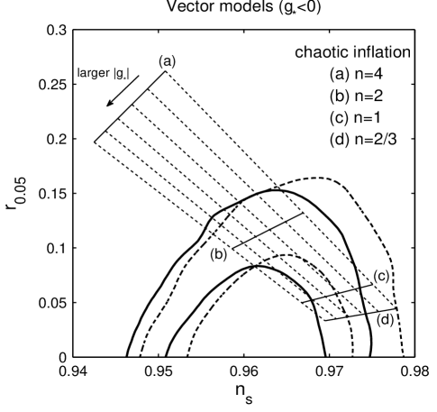
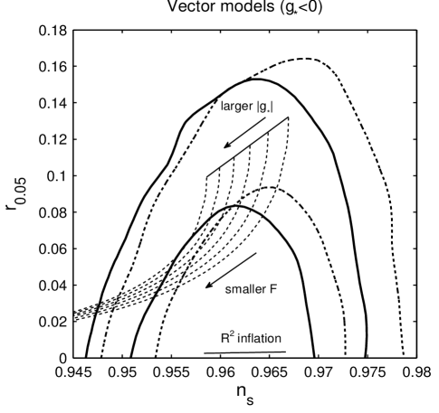
Figure 1: 2-dimensional observational bounds in the $(n_{s},r)$ plane with the number of e-foldings $N_{k}=60$ and the pivot wave number $k_{0}=0.05$ Mpc^-1. The bold solid curves represent the 68 % CL (inside) and 95 % CL (outside) boundaries derived by the joint data analysis of the Planck+WP+BAO+high-$\ell$ data, whereas the thick dashed curves correspond to the contours constrained by the Planck+WP+BAO data. In both cases the consistency relation $r(k_{0})=-8n_{t}(k_{0})$ is used. We consider several different inflaton potentials in the vector model, i.e., (i) $V(\phi)=\lambda\phi^{n}/n$ ($n=4,2,1,2/3$) (left), (ii) $V(\phi)=V_{0}[1+\cos(\phi/F)]$ (right), and (iii) $V(\phi)=(3/4)M^{2}M_{\rm pl}^{2}(1-e^{-\sqrt{2/3}\phi/M_{\rm pl}})^{2}$ (right), with $g_{*}$ ranging $-0.5\leq g_{*}\leq 0$. The thin dotted curves correspond to the anisotropic parameters $g_{*}=0,-0.1,-0.2,-0.3,-0.4,-0.5$, respectively. The thin line labelled as “$R^{2}$ inflation” shows the theoretical plots predicted by the potential (135). In the presence of the vector field, both $n_{s}$ and $r$ get smaller.

We also study natural inflation characterized by the potential Freese

$$V(\phi)=\Lambda^{4}\left[1+\cos(\phi/F)\right]\,,$$ (132)

where $\Lambda$ and $F$ are constants having a dimension of mass. The relation between $N_{k}$ and $\phi$ is given by $N_{k}=(2F^{2}/M_{\rm pl}^{2})\ln\left[\sin(\phi_{f}/(2F))/\sin(\phi/(2F))\right]$, where $\phi_{f}$ is known by solving the equation $\tan^{2}\left[\phi_{f}/(2F)\right]=2(F/M_{\rm pl})^{2}$. The observables (92) and (98) read

$$n_{s} = 1-\frac{3N_{k}M_{\rm pl}^{2}[3-\cos(\phi/F)]-\{2N_{k}M_{\rm pl}^{2}[3-\cos(\phi/F)]+4F^{2}[1+\cos(\phi/F)]\}g_{*}}{[1+\cos(\phi/F)]F^{2}N_{k}(3-2g_{*})}\,,$$ (133)

$$r = \frac{2\{12F^{2}[1+\cos(\phi/F)]-M_{\rm pl}^{2}[1-\cos(\phi/F)]g_{*}\}[1-\cos(\phi/F)]M_{\rm pl}^{2}}{[1+\cos(\phi/F)]^{2}F^{4}(3-2g_{*})}\,.$$ (134)

For a given value of $F$ we can numerically identify the field value $\phi$ corresponding to $N_{k}=60$. Then, we evaluate $n_{s}$ and $r$ according to the formulas (133) and (134). In the limit that $F\rightarrow\infty$, these observables approach the values (131) of chaotic inflation with $n=2$. In the right panel of Fig. 1, we show the theoretical values of $n_{s}$ and $r$ for different values of $F$ and $g_{*}$. For smaller $F$ and larger $|g_{*}|$, both $n_{s}$ and $r$ get smaller. When $g_{*}=0$, the mass scale $F$ is constrained to be $5.1M_{\rm pl}<F<7.9M_{\rm pl}$ (68 % CL) from the Planck+WP+BAO+high-$\ell$ data Kuro . For larger $|g_{*}|$, the allowed parameter space inside the 68 % CL contours tends to be narrower. In particular, if $|g_{*}|>0.5$, then the model is outside the 68 % CL boundary constrained by the Planck+WP+BAO+high-$\ell$ data. Thus, in natural inflation, the presence of anisotropic interactions leads to the deviation from the observationally favored region.

Let us also discuss the inflaton potential of the form

$$V(\phi)=\frac{3}{4}M^{2}M_{\rm pl}^{2}\left(1-e^{-\sqrt{2/3}\phi/M_{\rm pl}}\right)^{2}\,,$$ (135)

where $M$ is a constant having a dimension of mass. This potential arises in the Starobinsky’s model $f(R)=R+R^{2}/(6M^{2})$ Starobinsky after a conformal transformation to the Einstein frame with the field definition $\phi/M_{\rm pl}=\sqrt{3/2}\ln[\partial f(R)/\partial R]$ Maeda . Recently there have been numerous attempts to construct the potential (135) in the context of supergravity and quantum gravity Ketov . In the regime $\phi/M_{\rm pl}\gg 1$, the number of e-foldings is related to the inflaton, as $e^{-\sqrt{2/3}\phi/M_{\rm pl}}\simeq 3/(4N_{k})$ DeFelice . The slow-roll parameters are approximately given by $\epsilon\simeq 3/(4N_{k}^{2})$ and $\eta_{V}\simeq-1/N_{k}$, which means that $\epsilon$ is much smaller than $|\eta_{V}|$. Therefore, the observables (92) and (98) reduce to

$$n_{s}=1-\frac{2(3-4g_{*})}{N_{k}(3-2g_{*})}\,,\qquad r=\frac{9(8N_{k}^{2}-g_{*})}{2N_{k}^{4}(3-2g_{*})}\,.$$ (136)

When $g_{*}=0$ we have $n_{s}=1-2/N_{k}$ and $r=12/N_{k}^{2}$, which correspond to the values in the Starobinsky’s model Staper . The anisotropic interactions lead to the decrease of $n_{s}$, but still the model is well inside the 68 % CL contour, see the right panel of Fig. 1.

We also study hybrid inflation characterized by the potential $V(\phi)=\Lambda^{4}+m^{2}\phi^{2}/2$ hybrid , where $\Lambda$ and $m$ are constants. When $g_{*}=0$, this model gives rise to a blue-tilted spectrum ($n_{s}>1$). In the presence of anisotropic interactions it is possible to have a red-tilted spectrum, but we find that $n_{s}$ is larger than 0.99 for $|g_{*}|<0.5$. Hence the model is still outside the 95 % CL region.

IV.2 $f(\phi)^{2}H_{\mu\nu\lambda}H^{\mu\nu\lambda}$ model

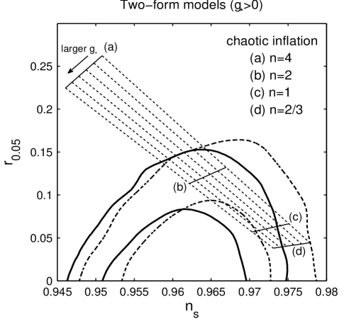
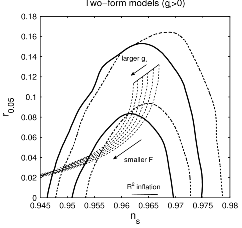
Figure 2: The same observational contours as those given in Fig. 1 (denoted as thick solid/dashed curves). The thin solid and dotted lines show the theoretical predictions of the two-form model with $N_{k}=60$ for three inflaton potentials (130), (132), and (135). We choose five different values of the anisotropic parameter: $g_{*}=0,0.1,0.2,0.3,0.4,0.5$. For larger $g_{*}$, both $n_{s}$ and $r$ get smaller.

In the two-form model the scalar spectral index and the tensor-to-scalar ratio, which are averaged over all the angles, are given by Eqs. (122) and (124), respectively.

For chaotic inflation characterized by the potential (130), these observables reduce to

$$n_{s}=1-\frac{6N_{k}(n+2)+2[N_{k}(n+6)+n]g_{*}}{N_{k}(n+4N_{k})(3+g_{*})}\,,\qquad r=\frac{48n}{(n+4N_{k})(3+g_{*})}\,.$$ (137)

In the left panel of Fig. 2 the theoretical predictions of chaotic inflation are shown for $g_{*}$ ranging in the region $0\leq g_{*}\leq 0.5$. For larger $g_{*}$ both $n_{s}$ and $r$ decrease, but the quadratic potential is outside the 68 % CL region. In the presence of anisotropic interactions the potentials with $n=1$ and $n=2/3$ enter the 95 % CL boundaries, but still these models are outside the 68 % CL region constrained by the Planck+WP+BAO+high-$\ell$ data. This shows that, for the same value of $|g_{*}|$, the power-law potentials with $n\leq 1$ in the two-form model are more difficult to be compatible with the data relative to the same potentials in the vector model.

For natural inflation given by the potential (132), the observables (122) and (124) read

$$n_{s} = 1-\frac{3N_{k}M_{\rm pl}^{2}[3-\cos(\phi/F)]+\{N_{k}M_{\rm pl}^{2}[3-\cos(\phi/F)]+2F^{2}[1+\cos(\phi/F)]\}g_{*}}{[1+\cos(\phi/F)]F^{2}N_{k}(3+g_{*})}\,,$$ (138)

$$r = \frac{24M_{\rm pl}^{2}[1-\cos(\phi/F)]}{F^{2}(3+g_{*})[1+\cos(\phi/F)]}\,,$$ (139)

which decrease for larger $g_{*}$ and smaller $F$. The difference from the vector model is that, for the same value of $|g_{*}|$, the allowed region of the two-form model inside the 68 % CL observational contours is wider. When $g_{*}=0.5$, for example, we find that the mass scale $F$ is constrained to be $5.9M_{\rm pl}<F<10.1M_{\rm pl}$ (68 % CL) in the two-form model. As long as $g_{*}$ is smaller than $1.0$, there are some allowed values of $F$ compatible with the observational data at 68 % CL.

For the potential (135) we have

$$n_{s}=1-\frac{2(3+2g_{*})}{N_{k}(3+g_{*})}\,,\qquad r=\frac{36}{N_{k}^{2}(3+g_{*})}\,.$$ (140)

As we see in the right panel of Fig. 2, this potential is well within the 68 % CL region.

We also find that hybrid inflation with the potential $V(\phi)=\Lambda^{4}+m^{2}\phi^{2}/2$ is outside the 95 % CL boundaries for $g_{*}<0.5$.

In summary, the observables $n_{s}$ and $r$ in the two-form model exhibit similar properties as those discussed in the vector model, but there are some potentials which can be inside and outside the 68 % CL region depending on the values of $g_{*}$. The precise observational bounds of $g_{*}$ (in particular the signs of $g_{*}$) will be able to distinguish the two anisotropic inflationary models further.

V Statistically anisotropic non-Gaussianities

In this section, we estimate anisotropic contributions to the statistical non-Gaussianities of curvature perturbations. The three-point correlation functions of $\zeta$ have been already derived both in the vector model Bartolo and in the two-form model Ohashi . In the vector model, Bartolo et al. Bartolo considered the squeezed shape in which the angles $\theta_{{\bm{k}}_{1},{\bm{k}}_{3}}$ and $\theta_{{\bm{k}}_{2},{\bm{k}}_{3}}$ between the momentum vectors satisfying the relation ${\bm{k}}_{1}+{\bm{k}}_{2}+{\bm{k}}_{3}=0$ are not necessarily close to $\pi/2$ and they took the average over angles to evaluate the local non-linear estimator $f_{\rm NL}^{\rm local}$. In the two-form model, the present authors Ohashi took the strict squeezed limit, $k_{3}\to 0$, $\theta_{{\bm{k}}_{1},{\bm{k}}_{3}}\to\pi/2$, $\theta_{{\bm{k}}_{2},{\bm{k}}_{3}}\to\pi/2$, and showed that $f_{\rm NL}^{\rm local}$ vanishes. We clarify the difference between these two approaches and estimate the local non-linear estimators in both analyses.

In the two-form model, the non-linear estimators have been also computed for other shapes of non-Gaussianities such as the equilateral and enfolded ones Ohashi . Since the similar analysis has not been yet done in the vector model, we evaluate $f_{\rm NL}$ in the equilateral and enfolded limits.

V.1 $f(\phi)^{2}F_{\mu\nu}F^{\mu\nu}$ model

In order to calculate the three-point correlation function of curvature perturbations in the vector model described by the action (2), we need to derive the Hamiltonian $H_{\zeta 2}$ following from the third-order interacting Lagrangian $L_{\rm int}^{(3)}\simeq 2a^{4}\delta E_{i}\delta E_{j}\zeta$, in addition to $H_{\zeta}$ given in Eq. (83). On using Eqs. (40) and (81), this interacting Hamiltonian is given by

$$H_{\zeta 2}=-\frac{2}{H^{4}\tau^{4}}\int\,\frac{d^{3}kd^{3}p}{(2\pi)^{3/2}}\,\delta{\cal E}_{i}({\bm{k}},\tau)\delta{\cal E}_{j}({\bm{p}},\tau)\hat{\zeta}^{(0)}(-{\bm{k}}-{\bm{p}},\tau)\,.$$ (141)

Then we can evaluate the three-point correlation of $\zeta$, as Bartolo

$$\delta\langle 0|\hat{\zeta}({\bm{k}}_{1})\hat{\zeta}({\bm{k}}_{2})\hat{\zeta}({\bm{k}}_{3})|0\rangle = i\int_{\tau_{{\rm min},1}}^{\tau}d\tau_{1}\int_{\tau_{{\rm min},2}}^{\tau_{1}}d\tau_{2}\,\int_{\tau_{{\rm min},3}}^{\tau_{2}}d\tau_{3}\,$$ (142)

$$\times\langle 0|\left[\left[\left[\hat{\zeta}^{(0)}({\bm{k}}_{1})\hat{\zeta}^{(0)}({\bm{k}}_{2})\hat{\zeta}^{(0)}({\bm{k}}_{3})(\tau),H_{\zeta 2}(\tau_{1})\right],H_{\zeta}(\tau_{2})\right]H_{\zeta}(\tau_{3})\right]|0\rangle+\text{2 perm.}$$

$$= \frac{4E_{x}^{2}}{27\epsilon^{3}M_{\rm pl}^{6}H^{6}}\prod_{i=1}^{3}\int_{-1/k_{i}}^{\tau}\frac{d\tau_{i}}{\tau_{i}^{4}}\left(\tau^{3}-\tau_{i}^{3}\right)$$

$$\times\int\,\frac{d^{3}p}{(2\pi)^{3/2}}\langle 0|\delta{\cal E}_{x}({\bm{k}}_{1},\tau_{1})\delta{{\cal E}}_{x}({\bm{k}}_{2},\tau_{2})\delta{\cal E}_{i}({\bm{p}},\tau_{3})\delta{{\cal E}}_{j}({\bm{k}}_{3}-{\bm{p}},\tau_{3})|0\rangle+\text{2 perm.}$$

$$\simeq 288\sqrt{2}\pi^{5/2}\frac{E_{x}^{2}}{\epsilon V}N_{k_{1}}N_{k_{2}}N_{k_{3}}({\cal P}_{\zeta}^{(0)})^{2}\delta^{(3)}({\bm{k}}_{1}+{\bm{k}}_{2}+{\bm{k}}_{3})$$

$$\times\left[\frac{1}{k_{1}^{3}k_{2}^{3}}(1-\cos^{2}\theta_{{\bm{k}}_{1},{\bm{x}}}-\cos^{2}\theta_{{\bm{k}}_{2},{\bm{x}}}+\cos\theta_{{\bm{k}}_{1},{\bm{x}}}\cos\theta_{{\bm{k}}_{2},{\bm{x}}}\cos\theta_{{\bm{k}}_{1},{\bm{k}}_{2}})+{\rm 2~{}perm.}\right].$$

The total anisotropic bispectrum ${\cal B}_{\zeta}$ is defined by $\delta\langle 0|\hat{\zeta}({\bm{k}}_{1})\hat{\zeta}({\bm{k}}_{2})\hat{\zeta}({\bm{k}}_{3})|0\rangle={\cal B}_{\zeta}\delta^{(3)}({\bm{k}}_{1}+{\bm{k}}_{2}+{\bm{k}}_{3})$. We introduce the non-linear estimator $f_{\rm NL}$ in the form

$${\cal B}_{\zeta}=\frac{3}{10}(2\pi)^{5/2}f_{\rm NL}({\cal P}_{\zeta})^{2}\sum_{i=1}^{3}k_{i}^{3}/\prod_{i=1}^{3}k_{i}^{3}\,,$$ (143)

by which $f_{\rm NL}$ for the vector model can be derived as Bartolo

$$f_{\rm NL} = 480\,r_{A}\frac{({\cal P}_{\zeta}^{(0)})^{2}}{({\cal P}_{\zeta})^{2}}\frac{N_{k_{1}}N_{k_{2}}N_{k_{3}}}{k_{1}^{3}+k_{2}^{3}+k_{3}^{3}}[k_{3}^{3}(1-\cos^{2}\theta_{{\bm{k}}_{1},{\bm{x}}}-\cos^{2}\theta_{{\bm{k}}_{2},{\bm{x}}}+\cos\theta_{{\bm{k}}_{1},{\bm{x}}}\cos\theta_{{\bm{k}}_{2},{\bm{x}}}\cos\theta_{{\bm{k}}_{1},{\bm{k}}_{2}})+{\rm 2~{}perm.}]$$ (144)

$$\simeq 60\left(\frac{-g_{*}}{0.1}\right)\left(\frac{N_{k}}{60}\right)\frac{1}{k_{1}^{3}+k_{2}^{3}+k_{3}^{3}}[k_{3}^{3}(1-\cos^{2}\theta_{{\bm{k}}_{1},{\bm{x}}}-\cos^{2}\theta_{{\bm{k}}_{2},{\bm{x}}}+\cos\theta_{{\bm{k}}_{1},{\bm{x}}}\cos\theta_{{\bm{k}}_{2},{\bm{x}}}\cos\theta_{{\bm{k}}_{1},{\bm{k}}_{2}})+{\rm 2~{}perm.}],$$

where, in the first line, we used $\rho_{A}=E_{x}^{2}/2$ and the quantity $r_{A}$ defined in Eq. (17). In the second line we employed the approximations $({\cal P}_{\zeta})^{2}\simeq({\cal P}_{\zeta}^{(0)})^{2}$, $N_{k_{1}}\simeq N_{k_{2}}\simeq N_{k_{3}}\equiv N_{k}$, and the definition of $g_{*}$ given in Eq. (89).

Let us first take the same approach as that used in Ref. Ohashi for the two-form model. It is convenient to introduce the following parameters

$$r_{2}\equiv\frac{k_{2}}{k_{1}}\,,\quad r_{3}\equiv\frac{k_{3}}{k_{1}}\,.$$ (145)

If we fix $r_{2}=1$ and define the angles $\beta=\pi-\theta_{{\bm{k}}_{1},{\bm{k}}_{2}}$ and $\gamma=\theta_{{\bm{k}}_{1},{\bm{x}}}$, it follows that

$$f_{\rm NL} \simeq 60\left(\frac{-g_{*}}{0.1}\right)\left(\frac{N_{k}}{60}\right)\frac{1}{2+r_{3}^{3}}\biggl{[}\frac{1}{2}-r_{3}^{3}\cos\beta(\sin\beta\sin\gamma\cos\gamma-\cos\beta+\cos\beta\cos^{2}\gamma)-\cos^{2}\beta\cos^{2}\gamma$$ (146)

$$~{}~{}~{}~{}~{}~{}~{}~{}~{}~{}~{}~{}~{}~{}~{}~{}~{}~{}~{}~{}~{}~{}~{}~{}~{}~{}~{}~{}~{}~{}~{}~{}~{}+\frac{1}{2}\cos^{2}\beta+\cos\beta\cos^{2}\gamma-\cos\beta\sin\beta\cos\gamma\sin\gamma-\cos\beta+\sin\beta\sin\gamma\cos\gamma\biggr{]}.$$

The angle $\beta$ is in the range $0<\beta<\pi$ (i.e., $0<r_{3}<2$). In the strict squeezed limit ($r_{3}\to 0$ and $\beta\to 0$), the local estimator $f_{\rm NL}^{\rm local}$ vanishes for any values of $\gamma$. This limit corresponds to the case in which the angles $\theta_{{\bm{k}}_{2},{\bm{k}}_{3}}$ and $\theta_{{\bm{k}}_{3},{\bm{k}}_{1}}$ approach $\pi/2$.

Bartolo et al. Bartolo estimated $f_{\rm NL}^{\rm local}$ in the following way. For the incomplete squeezed shape the angles $\theta_{{\bm{k}}_{2},{\bm{k}}_{3}}$ and $\theta_{{\bm{k}}_{3},{\bm{k}}_{1}}$ are not necessarily close to $\pi/2$. In other words, unless we take the strict squeezed limit ${\bm{k}}_{1}\to-{\bm{k}}_{2}$, we can consider any angle between ${\bm{k}}_{3}$ and ${\bm{k}}_{1},{\bm{k}}_{2}$. Averaging over $f_{\rm NL}$ in all the directions along the same line as Eq. (91), the local estimator for the squeezed shape ($k_{3}\ll k_{1}\simeq k_{2}$, $\theta_{{\bm{k}}_{1},{\bm{k}}_{3}}\to\pi-\theta_{{\bm{k}}_{2},{\bm{k}}_{3}}$, and $\theta_{{\bm{k}}_{2},{\bm{x}}}\to\pi-\theta_{{\bm{k}}_{1},{\bm{x}}}$) reads

$$f_{\rm NL}^{\rm local,average}\simeq 27\left(\frac{-g_{*}}{0.1}\right)\left(\frac{N_{k}}{60}\right)\frac{[1-\cos^{2}\theta_{{\bm{k}}_{1},{\bm{x}}}-\cos^{2}\theta_{{\bm{k}}_{3},{\bm{x}}}+\cos\theta_{{\bm{k}}_{1},{\bm{x}}}\cos\theta_{{\bm{k}}_{3},{\bm{x}}}\cos\theta_{{\bm{k}}_{1},{\bm{k}}_{3}}]}{4/9}\,,$$ (147)

where we used the fact that the average value of the function in the last square bracket integrated over all the angles is $4/9$. In this analysis the local non-linear estimator does not vanish and it can be as large as the order of $10$ for $g_{*}\sim-0.1$.

The Planck group placed the bound on the local non-linear estimator to be $f_{\rm NL}^{\rm local}=2.7\pm 5.8$ (68 % CL) Adenon , but we cannot literally use this bound to constrain the anisotropic inflationary models. As we have seen above, the local non-Gaussianities depend on what kind of squeezed shapes to be taken in the data analysis. It is interesting that the strict or incomplete squeezed shapes do matter to estimate the level of non-Gaussianities correctly. The detailed data analysis based on different squeezed shapes is beyond the scope of our paper.

Using the result (146), we can calculate the non-linear estimator for the shapes other than the squeezed one. In the equilateral ($\beta\rightarrow\pi/3\,,r_{3}\rightarrow 1$) and the enfolded ($\beta\rightarrow\pi\,,r_{3}\rightarrow 2$) limits, we have

$$f_{\rm NL}^{\rm equil} \simeq 7.5\left(\frac{-g_{*}}{0.1}\right)\left(\frac{N_{k}}{60}\right)\,,$$ (148)

$$f_{\rm NL}^{\rm enfolded} \simeq 60\left(\frac{-g_{*}}{0.1}\right)\left(\frac{N_{k}}{60}\right)\sin^{2}\gamma\,.$$ (149)

Unlike the squeezed case, these estimators do not depend on how we take the limits of equilateral and enfolded shapes. The equilateral non-linear estimator is independent of the angle $\gamma$ and it is typically of the order of $1$ for $|g_{*}|\lesssim 0.1$. Meanwhile, $f_{\rm NL}^{\rm enfolded}$ depends on $\gamma$ and it has a maximum at $\gamma=\pi/2$. The maximum value of $f_{\rm NL}^{\rm enfolded}$ can be as large as $60$ for $|g_{*}|\sim 0.1$, which is an interesting signature of the vector model.

V.2 $f(\phi)^{2}H_{\mu\nu\lambda}H^{\mu\nu\lambda}$ model

In the two-form model the Hamiltonian following from the third-order interacting Lagrangian $L_{\rm int}^{(3)}\simeq a^{4}\delta E_{ij}\delta E_{ij}\zeta/2$ is given by

$$H_{\zeta 2}=-\frac{1}{2H^{4}\tau^{4}}\int\,\frac{d^{3}kd^{3}p}{(2\pi)^{3/2}}\,\delta{\cal E}_{ij}({\bm{k}},\tau)\delta{\cal E}_{ij}({\bm{p}},\tau)\hat{\zeta}^{(0)}(-{\bm{k}}-{\bm{p}},\tau)\,.$$ (150)

The three-point correlation function of $\zeta$ can be computed by using the interacting Hamiltonians (115) and (150) in the way similar to the derivation of Eq. (142). In Ref. Ohashi this was already derived as

$$\delta\langle 0|\hat{\zeta}({\bm{k}}_{1})\hat{\zeta}({\bm{k}}_{2})\hat{\zeta}({\bm{k}}_{3})|0\rangle=36\sqrt{2}\pi^{5/2}\frac{E_{yz}^{2}}{\epsilon V}N_{k_{1}}N_{k_{2}}N_{k_{3}}({\cal P}_{\zeta}^{(0)})^{2}\delta^{(3)}({\bm{k}}_{1}+{\bm{k}}_{2}+{\bm{k}}_{3})\left[\frac{\cos\theta_{{\bm{k}}_{1},{\bm{k}}_{2}}\cos\theta_{{\bm{k}}_{1},{\bm{x}}}\cos\theta_{{\bm{k}}_{2},{\bm{x}}}}{k_{1}^{3}k_{2}^{3}}+\text{2 perm.}\right].$$ (151)

From the definition (143) of $f_{\rm NL}$, it follows that

$$f_{\rm NL} \simeq 30\left(\frac{g_{*}}{0.1}\right)\left(\frac{N_{k}}{60}\right)\frac{1}{k_{1}^{3}+k_{2}^{3}+k_{3}^{3}}[k_{3}^{3}\cos\theta_{{\bm{k}}_{1},{\bm{k}}_{2}}\cos\theta_{{\bm{k}}_{1},{\bm{x}}}\cos\theta_{{\bm{k}}_{2},{\bm{x}}}+k_{1}^{3}\cos\theta_{{\bm{k}}_{2},{\bm{k}}_{3}}\cos\theta_{{\bm{k}}_{2},{\bm{x}}}\cos\theta_{{\bm{k}}_{3},{\bm{x}}}$$ (152)

$$~{}~{}~{}~{}~{}~{}~{}~{}~{}~{}~{}~{}~{}~{}~{}~{}~{}~{}~{}~{}~{}~{}~{}~{}~{}~{}~{}~{}~{}~{}~{}~{}~{}~{}~{}~{}~{}~{}~{}+k_{2}^{3}\cos\theta_{{\bm{k}}_{3},{\bm{k}}_{1}}\cos\theta_{{\bm{k}}_{3},{\bm{x}}}\cos\theta_{{\bm{k}}_{1},{\bm{x}}}]\,,$$

where we used the anisotropic parameter $g_{*}$ given in Eq. (121) with $r_{B}=E_{yz}^{2}/(2\epsilon V)$.

For the squeezed shape, if we take the average over angles as the derivation of Eq. (147), the local non-linear parameter reads

$$f_{\rm NL}^{\rm local,average}\simeq 3.3\left(\frac{g_{*}}{0.1}\right)\left(\frac{N_{k}}{60}\right)\frac{[\cos\theta_{{\bm{k}}_{1},{\bm{x}}}\cos\theta_{{\bm{k}}_{3},{\bm{x}}}\cos\theta_{{\bm{k}}_{1},{\bm{k}}_{3}}]}{1/9}\,,$$ (153)

where the value $1/9$ is the total spatial average of the function in the last square bracket. Therefore, $f_{\rm NL}^{\rm local,average}$ dose not vanish in this analysis. We note that $f_{\rm NL}^{\rm local,average}$ in this case is smaller than that in the vector model by one order of magnitude, see Eq. (147). Thus the local non-Gaussianities averaged over all the directions can allow us to discriminate between the vector and the two-form models. On the other hand, in the strict squeezed limit characterized by $k_{3}\to 0$, $\theta_{{\bm{k}}_{2},{\bm{k}}_{3}}\to\pi/2$, and $\theta_{{\bm{k}}_{3},{\bm{k}}_{1}}\to\pi/2$, the non-linear estimator (152) vanishes, $f_{\rm NL}^{\rm local}=0$ Ohashi .

The non-linear parameters in the equilateral and the enfolded limits were already evaluated in Ref. Ohashi by considering a configuration with $k_{1}=k_{2}$ and $\beta=\pi-\theta_{{\bm{k}}_{1},{\bm{k}}_{2}}$, $\gamma=\theta_{{\bm{k}}_{1},{\bm{x}}}$. They are given, respectively, by

$$f_{\rm NL}^{\rm equil} \simeq 3.7\left(\frac{g_{*}}{0.1}\right)\left(\frac{N_{k}}{60}\right)\,,$$ (154)

$$f_{\rm NL}^{\rm enfolded} \simeq 30\left(\frac{g_{*}}{0.1}\right)\left(\frac{N_{k}}{60}\right)\cos^{2}\gamma\,.$$ (155)

The equilateral non-linear estimator is independent of $\gamma$, but the enfolded one depends on $\gamma$. Unlike the vector model, $f_{\rm NL}^{\rm enfolded}$ has a maximum at $\gamma=0$ or $\pi$. Both $f_{\rm NL}^{\rm equil}$ and $f_{\rm NL}^{\rm enfolded}$ are about half times smaller than those in the vector model. In general, for the same values of $|g_{*}|$, the two-form model is easier to satisfy observational bounds of non-Gaussianities relative to the vector model.

VI Conclusions

We have studied differences between two anisotropic inflationary scenarios paying particular attention to their observational signatures. In the presence of a vector or a two-form field coupled to the inflaton, there exist background solutions along which the anisotropic hairs survive during inflation. In the vector model the anisotropic shear $\Sigma$ divided by the Hubble rate $H$ is given by Eq. (18) for the coupling (12), while in the two-form model it is given by Eq. (33) for the coupling (30). The opposite signs of $\Sigma/H$ between the two models reflect the fact that the types of anisotropies are different (either oblate or prolate).

In the presence of anisotropic interactions, we have computed the power spectra of scalar/tensor perturbations and the resulting spectral indices convenient to confront with the CMB observations. The different types of anisotropies affect the sign of $g_{*}$ appearing in the scalar power spectrum defined by Eq. (1), i.e., $g_{*}<0$ in the vector model and $g_{*}>0$ in the two-form model. The anisotropic contributions to the isotropic tensor power spectrum are suppressed relative to those to the isotropic scalar one. In particular, in the two-form model, we showed that anisotropic interactions do not give rise to any corrections to the isotropic tensor power spectrum.

We have computed the two-point cross correlations between curvature perturbations and gravitational waves. While the cross correlation remains in the vector model, we find that it vanishes in the two-form model. The latter property may reflect the fact that, unlike the vector field, the two-form field can be mapped to the form of a scalar field. The different signatures of the two anisotropic models will be useful to discriminate between those models in future observations of the TB power spectrum.

In the light of the recent Planck data, we have placed observational constraints on several different inflaton potentials from the information of the scalar spectral index $n_{s}$ and the tensor-to-scalar ratio $r$. In both the vector and two-form models anisotropic interactions lead to the enhancement of the scalar power spectrum on larger scales, by which both $n_{s}$ and $r$ decrease for any inflaton potentials. In the vector model, we found that the potentials $V(\phi)=\lambda\phi$ and $V(\phi)=(3\lambda/2)\phi^{2/3}$ show the better compatibility with the data for larger $|g_{*}|$ and that the potential of natural inflation is outside the 68 % CL region constrained by the Planck+WP+BAO+high-$\ell$ data for $|g_{*}|\gtrsim 0.5$. In the two-form model, the level of the decreases of $n_{s}$ and $r$ is less significant relative to the vector model for the same values of $|g_{*}|$. The potential (135), which originates from the Starobinsky’s $f(R)$ model, is well inside the 68 % CL region even in the presence of anisotropic interactions with $|g_{*}|<0.5$.

We also compared the three-point correlation functions of curvature perturbations between the two anisotropic inflationary scenarios. If the strict squeezed limit characterized by $k_{3}\to 0$, $\theta_{{\bm{k}}_{1},{\bm{k}}_{3}}\to\pi/2$, and $\theta_{{\bm{k}}_{2},{\bm{k}}_{3}}\to\pi/2$ is taken, the local non-linear estimators $f_{\rm NL}^{\rm local}$ vanish in both the vector and the two-form models. However, for the squeezed shape where the angles $\theta_{{\bm{k}}_{1},{\bm{k}}_{3}}$ and $\theta_{{\bm{k}}_{2},{\bm{k}}_{3}}$ are not necessarily close to $\pi/2$, the non-linear estimator averaged over all the directions is given by Eq. (147) in the vector model and by Eq. (153) in the two-form model. The former is larger than the latter by one order of magnitude for the same order of the anisotropic parameter $g_{*}$. We also evaluated the non-linear estimators in the equilateral and enfolded limits and found that $f_{\rm NL}$ in the vector model is about twice larger than that in the two-form model for the same values of $|g_{*}|$. In general, the two-form model is easier to satisfy observational bounds of non-Gaussianities relative to the vector model.

We have thus shown that the two anisotropic inflationary scenarios can be distinguished from each other by evaluating several CMB observables. In particular, the precise measurements of $g_{*}$ as well as the TB correlation will clarify which anisotropic model is favored over the other.