Improved dynamics and gravitational collapse of tachyon field
coupled with a barotropic fluid

Abstract

We consider a spherically symmetric gravitational collapse of a tachyon field with an inverse square potential, which is coupled with a barotropic fluid. By employing an holonomy correction imported from loop quantum cosmology, we analyse the dynamics of the collapse within a semiclassical description. Using a dynamical system approach, we find that the stable fixed points given by the standard general relativistic setting turn into saddle points in the present context. This provides a new dynamics in contrast to the black hole and naked singularities solutions appearing in the classical model. Our results suggest that classical singularities can be avoided by quantum gravity effects and are replaced by a bounce. By a thorough numerical studies we show that, depending on the barotropic parameter $\gamma$, there exists a class of solutions corresponding to either a fluid or a tachyon dominated regimes. Furthermore, for the case $\gamma\sim 1$, we find an interesting tracking behaviour between the tachyon and the fluid leading to a dust-like collapse. In addition, we show that, there exists a threshold scale which determines when an outward energy flux emerges, as a non-singular black hole is forming, at the corresponding collapse final stages.

I Introduction

The spherically symmetric gravitational collapse, with a variety of matter fields, has been well studied in general relativity (see Ref. Joshi:2007 and references therein). Those investigations indicate that the gravitational collapse, depending on the initial conditions, may produce a black hole with a singularity inside or a naked singularity as its final state (Joshi:2007, ; Penrose:1965, ; Hawking:1974, ). However, these results are not expected to hold in a quantum theory of gravity. Among the candidates for a theory of quantum gravity, loop quantum gravity (LQG) (Ashtekar:2004, ; LQC-AS, ; Bojowald:2010, ; Ashtekar:2005, ) is a non-perturbative background independent theory. From the effective constraints approach used in the LQG program, there are two general types of quantum corrections, namely the ‘inverse triad’ and ‘holonomy’ types.

The study of the gravitational collapse has thus been considered in LQG, by means of these corrections. It was proposed that inverse triad modifications resolve the classical singularities that arise at the final state of the gravitational collapse, whose matter source is a standard scalar field (Bojowald:2005, ; Goswami:2006, ). Moreover, in a homogeneous and spherically symmetric model, loop gravity effects, within a holonomy correction, modify the standard Friedmann equation by adding a $-\rho^{2}/\rho_{{\rm crit}}$ correction term into it. In a cosmological context, these effects resolve the big bang singularity and replace it by a bounce Ashtekar:2006 . In addition, for gravitational collapse of a scalar field us:2013c , with non-interacting particles (dust) and a perfect fluid describing radiation Modesto:2013 , it was shown that those quantum gravity effects provide a threshold scale for a non-singular black hole formation.

More recently, the gravitational collapse of a self interacting tachyon field coupled with a barotropic fluid has been considered in a classical context us:2013a , exploring the non-canonical features of the tachyon kinetic term and its subsequent (anti)friction effects. Therein, a dynamical system analysis was employed, where, by making use of the specific kinematical features of the tachyon field (which are rather different from a standard scalar field), it was established the initial conditions for which either the tachyon or the fluid becomes dominant. It was found the conditions under which a black hole or a naked singularity scenarios are produced, as well as solutions with a tracking behaviour between the tachyon and the fluid.

A tachyon scalar field has also been investigated in loop quantum cosmology (LQC) as a concrete example for investigating the initial singularity of the universe Li:2009 . In the context of a gravitational collapse, by employing quantum gravity effects of the inverse triad type, it was proposed that the geometry of space-time near the classical singularity is regular us:2013b . Furthermore, some novel features such as evaporation of the horizons in the presence of the inverse triad modifications were studied. Nevertheless, holonomy type correction can bring, in the context of homogeneous LQC, distinct and interesting physical aspects when compared with the inverse triad type. Therefore, it is of interest to investigate how a modification provided by holonomy corrections to the tachyon equations of motion can avoid the classical singularity that may arise at the final state of the gravitational collapse. In addition, another question that can be addressed here is how this type of loop quantum effect can indeed affect the emergence of trapped surfaces in this kind of models. These questions constitute our main goal to be explored in this paper.

The organization of this paper is as follows. In section II we employ the loop gravity effects with holonomy corrections to the gravitational collapse of a tachyon field in addition with a barotropic fluid. Then, in section III we present a phase space analysis for our semiclassical model and will find the possible fixed point solutions to the evolution equations. This analysis provides a correspondence between the fixed point solutions found in the herein semiclassical regime and those given by their general relativistic counterpart presented in Ref. us:2013a . Nevertheless, it will be shown that the corresponding loop gravity modified fixed point solutions, due to the holonomy effects, are free of the central singularity whereas their classical counterpart are not. In section IV, by using numerical techniques, we will study the evolution of trapped surfaces in the semiclassical interior space-time of the collapse. This analysis will further provide a contrasting between our herein semiclassical analysis and the one given by the inverse triad modified collapsing scenario presented in Ref. us:2013b . Finally, in section V we present the conclusion and discussion of our work.

II Gravitational collapse: Improved dynamics

We consider a spherically symmetric gravitational collapse whose interior space-time is the marginally bound case, i.e., the $k=0$ FLRW us:2013a . Let $t$ be the proper time for a falling observer whose geodesic trajectories are labeled by the comoving radial coordinate $r$, and $R(t,r):=ra(t)$ is the area radius of the collapsing cloud. Then, for a continuous collapsing scenario, we take $\dot{R}=r\dot{a}<0$ (with a ‘dot’ denoting a derivative with respect to the proper time $t$), implying that the area radius of the collapsing shell, for a constant $r$, decreases monotonically.

The corresponding Hamiltonian constraint for the interior geometry is provided as Ashtekar:2005

$${\cal H}\ =\ -\frac{3}{\kappa\tilde{\gamma}^{2}}c^{2}\sqrt{|p|}+{\cal H}_{{\rm matt}}\ ,$$ (1)

where $c:=\tilde{\gamma}\dot{a}<0$ and $p:=a^{2}$ are, respectively, the conjugate connection and triad satisfying the non-vanishing Poisson bracket $\{c,p\}=\kappa\tilde{\gamma}/3$, with $\tilde{\gamma}\approx 0.23$ being the Barbero-Immirzi dimensionless parameter. Moreover, $\kappa=8\pi G$, and ${\cal H}_{{\rm matt}}=\rho V$ is the matter Hamiltonian with $V$ being the volume of the fiducial cell Ashtekar:2005 .

A pertinent scenario to investigate semiclassically effects suggested from LQG (as far as a gravitational collapse is concerned) is the so-called holonomy correction. The algebra generated by the holonomy of phase space variables $c$ is just the algebra of the almost periodic function of $c$, i.e., $e^{i\bar{\mu}c/2}$ where $\bar{\mu}$ is inferred as kinematical length of the square loop, since its dimension is similar to that of a length, which together with $p$, constitutes the fundamental canonical variables in quantum theory Ashtekar:2005 . This consists semiclassically in replacing $c$ in Eq. (1), with the phase space function, by means of

$$\frac{1}{2i\bar{\mu}}\left(e^{i\bar{\mu}c}-e^{-i\bar{\mu}c}\right)=\frac{\sin(\bar{\mu}c)}{\bar{\mu}}~{}.$$ (2)

It is expected that the classical theory is recovered for small $\bar{\mu}$; we therefore obtain the effective semiclassical Hamiltonian (Ashtekar:2006, ; Taveras:2006, )

$${\cal H}_{{\rm eff}}\ =\ -\frac{3}{\kappa\tilde{\gamma}^{2}\bar{\mu}^{2}}\sqrt{|p|}\sin^{2}(\bar{\mu}c)+{\cal H}_{\mathrm{matt}}\ .$$ (3)

The dynamics of the fundamental variables is then obtained by solving the system of Hamilton equations; i.e.,

$$\dot{p} \ =\ \{p,{\cal H}_{{\rm eff}}\}=-\frac{\kappa\tilde{\gamma}}{3}\frac{\partial{\cal H}_{{\rm eff}}}{\partial c}$$

$$\ =\ \frac{2a}{\tilde{\gamma}\bar{\mu}}\sin(\bar{\mu}c)\cos(\bar{\mu}c).$$ (4)

Furthermore, the vanishing Hamiltonian constraint (3) implies that

$$\sin^{2}(\bar{\mu}c)\ =\ \frac{\kappa\tilde{\gamma}^{2}\bar{\mu}^{2}}{3a}{\cal H}_{{\rm matt}}\ .$$ (5)

Thus, using Eqs. (4) and (5), we subsequently obtain the modified Friedmann equation, $H=\dot{a}/a=\dot{p}/2p$ :

$$H^{2}\ =\ \frac{\kappa}{3}\rho\left(1-\frac{\rho}{\rho_{\text{crit}}}\right),$$ (6)

where $\rho_{{\rm crit}}=3/(\kappa\tilde{\gamma}^{2}\lambda^{2})\approx 0.41\rho_{{\rm Pl}}$, and $\rho$ is the total (classical) energy density of the collapse matter content. Eq. (6) implies that the classical energy density $\rho$ is limited to the interval $\rho_{0}<\rho<\rho_{{\rm crit}}$ having an upper bound at $\rho_{{\rm crit}}$, where $\rho_{0}\ll\rho_{{\rm crit}}$ is the energy density of the star at the initial configuration, $t=0$. Hence, the effective energy density reads

$$\rho_{{\rm eff}}\ :=\ \rho\left(1-\frac{\rho}{\rho_{{\rm crit}}}\right).$$ (7)

We see that the effective scenario, provided by holonomy corrections, leads to a $-\rho^{2}$ modification of the energy density, which becomes important when the energy density becomes comparable to $\rho_{{\rm crit}}$. In the limit $\rho\rightarrow\rho_{{\rm crit}}$, the Hubble rate vanishes; a classical singularity is thus replaced by a bounce.

From Eq. (6) the time derivative of the Hubble rate reads

$$\dot{H}\ =\ -\frac{\kappa}{2}(\rho+p)\left(1-2\frac{\rho}{\rho_{{\rm crit}}}\right),$$ (8)

Then, using the relation $\ddot{a}/a=\dot{H}+H^{2}$ we obtain the modified Raychaudhuri equation as

$$\frac{\ddot{a}}{a}\ =\ -\frac{\kappa}{6}\>\rho\left(1-4\frac{\rho}{\rho_{{\rm crit}}}\right)-\frac{\kappa}{2}\>p\left(1-2\frac{\rho}{\rho_{{\rm crit}}}\right).$$ (9)

By redefinition of the Raychaudhuri equation (9), similar to the corresponding classical relation, in an effective form $\ddot{a}/a=-\kappa/6(\rho_{\rm eff}+3p_{\rm eff})$, we obtain the effective pressure $p_{\rm eff}$ of the system as (Ashtekar:2006, ; Taveras:2006, )

$$p_{\text{eff}}\ =\ p\left(1-2\frac{\rho}{\rho_{{\rm crit}}}\right)-\frac{\rho^{2}}{\rho_{{\rm crit}}}\ .$$ (10)

The effective energy density $\rho_{{\rm eff}}$ and pressure $p_{{\rm eff}}$ satisfy the conservation equation:

$$\dot{\rho}_{\text{eff}}+3H(\rho_{\text{eff}}+p_{\text{eff}})=0\ .$$ (11)

We can define the effective equation of state as

$$w_{{\rm eff}}\ :=\ \frac{p_{{\rm eff}}}{\rho_{{\rm eff}}}\ =\ \frac{p}{\rho}\left(\frac{\rho_{{\rm crit}}-2\rho}{\rho_{{\rm crit}}-\rho}\right)-\frac{\rho}{\rho_{{\rm crit}}-\rho}\ .$$ (12)

In general relativity, the equation for an apparent horizon in a spherical symmetric space-time is given by $g^{ij}R_{,i}R_{,j}=0$, which corresponds to $F/R=1$; the $F(R)=\kappa\rho R^{3}/3$ is the mass function of the collapsing matter. Thus, the space-time is said to be trapped or untrapped if $F>R$ or $F<R$, respectively Joshi:2007 . Since in the considered effective scenario, the energy density $\rho$ in the Friedmann equation (6) is modified as $\rho_{{\rm eff}}$, hence, the mass function $F(R)$ should be modified in the herein semiclassical regime and can be written in the following form us:2013c :

$$F_{{\rm eff}}\ =\ \frac{\kappa}{3}\rho_{{\rm eff}}R^{3}\ =\ F\left(1-\frac{\rho}{\rho_{{\rm crit}}}\right).$$ (13)

We followed a possible perspective in effective scenario in which, the phase space trajectories are considered to have classical form whereas the matter components take effective form due to quantum effects. The $\rho/\rho_{{\rm crit}}$ term in Eq. (13) can be written as

$$\frac{\rho}{\rho_{{\rm crit}}}\ =\ \frac{a_{{\rm min}}^{3}}{a^{3}}\frac{F}{F_{{\rm crit}}}\ ,$$ (14)

where $a_{{\rm min}}$ and $F_{{\rm crit}}:=(\kappa/3)\rho_{{\rm crit}}r^{3}a_{{\rm min}}$ are respectively, values of the scale factor and mass function at the bounce. It is seen from Eq. (14) that, the mass function $F$ changes in the interval $F_{0}\leq F\leq F_{{\rm crit}}$ along with the collapse dynamical evolution, so that, it remains finite during the semiclassical regime; $F_{0}=(\kappa/3)\rho_{0}r^{3}a_{0}^{3}$ is the initial value for the mass function at $t=0$. Furthermore, the effective mass function (13) vanishes at the bounce.

We should notice that the effective mass function (13), likewise the effective energy density and pressure, must be consistent with the continuity equation (11). By working out the relations (13), (7) and (10), using the conservation equation (11), we find the following effective equations describing the dynamics of our semiclassical gravitational collapse:

$$\kappa\rho_{\rm eff}=\frac{F_{{\rm eff},r}}{R^{2}R_{,r}}\ ,\quad\kappa p_{\rm eff}=-\frac{\dot{F}_{{\rm eff}}}{R^{2}\dot{R}}\ ,\quad\dot{R}^{2}=\frac{F_{\rm eff}}{R}\ ,$$ (15)

with ‘$,r$’ denoting the derivative with respect to $r$. In the classical limit where $\rho/\rho_{\rm crit}\ll 1$, we have that $\rho_{\rm eff}\rightarrow\rho$;  $p_{\rm eff}\rightarrow p$ and $F_{\rm eff}\rightarrow F$, then, Eq. (15) reduces to the known Einsein’s equations for gravitational collapse Joshi:2007 .

Let us follow Refs. (us:2013a, ; us:2013b, ) and consider the total energy density, $\rho$, of the collapse to be

$$\rho\ =\ \rho_{\phi}+\rho_{\gamma}\ ,$$ (16)

which constitutes the classical energy densities of the tachyon field and the barotropic fluid. In a strictly classical setting, the energy density $\rho_{\phi}$ and pressure $p_{\phi}$ of the tachyon field are given by

$$\rho_{\phi}=\frac{V(\phi)}{\sqrt{1-\dot{\phi}^{2}}},~{}~{}~{}~{}p_{\phi}=-V(\phi)\sqrt{1-\dot{\phi}^{2}}\ ,$$ (17)

where $V(\phi)$ is the tachyon potential. Furthermore, the energy density of the barotropic fluid, $\rho_{\gamma}$, reads

$$\rho_{\gamma}\ =\ \rho_{\gamma 0}\left(\frac{a}{a_{0}}\right)^{-3\gamma},$$ (18)

where $\rho_{\gamma 0}$ is a positive constant denoting the fluid density at the initial configuration, $a_{0}$, of the collapse, and $\gamma$ is an adiabatic index satisfying $p_{\gamma}=(\gamma-1)\rho_{\gamma}$, with $p_{\gamma}$ being the pressure of the barotropic fluid.

For a physically reasonable matter content for the collapsing cloud, the tachyon field and the barotropic fluid would have to satisfy the weak and dominant energy conditions. It is straightforward to show that the tachyon matter satisfies the weak and dominant energy conditions. For a fluid with the barotropic parameter $\gamma>0$, the weak energy condition is satisfied, however, concerning the dominant energy condition, it follows that $\gamma$ must hold the range $\gamma\leq 2$ us:2013a .

From the total energy conservation equation for collapse matter source, we could write, generally, that

$$\dot{\rho}_{\phi}+3H(1+w_{\phi})\rho_{\phi}=-\Gamma_{{\rm int}}\ ,$$ (19)

$$\dot{\rho}_{\gamma}+3\gamma H\rho_{\gamma}=+\Gamma_{{\rm int}}\ ,$$ (20)

where the function $\Gamma_{{\rm int}}$ denotes the interaction between the tachyon and fluid. A natural interpretation of $\Gamma_{{\rm int}}$ is that it implies an energy transfer between the tachyon field and the barotropic fluid. Such cases were studied in (classical) cosmological scenarios where two fluid system drive an accelerating universe TB-Int1 ; TB-Int2 ; TB-Int3 . Our main goal in this paper is to investigate the effects of LQG holonomy corrections to the tachyon equations of motion, and consequently, the emergence of trapped surfaces in the herein semiclassical collapse. Furthermore, we will discuss the situation in which only a tachyon matter or a fluid is present. Thus, our approach will be to consider the non-interacting case to fully access the underlying dynamics. However, it is expected that for the interacting case the main features of the bouncing scenario will remain unchanged. But, allowing a situation where the tachyon field and the barotropic fluid no longer obey a local conservation equation, might certainly change the outcome of the horizon formation in the presence of the interaction term. When we find the solutions for the non-interacting case, we may get a general idea of how the presence of the interaction term can affect our outcome, however, a full independent analysis will be required to describe the dynamics of the collapse in the case of interacting tachyon matter. In the present context, we thus only assume that the tachyon field is self interacting, i.e., $\Gamma_{{\rm int}}=0$. The conservation energy density (19) for the tachyon field gives

$$\ddot{\phi}=-\left(1-\dot{\phi}^{2}\right)\left[3H\dot{\phi}+\frac{V_{,\phi}}{V}\right],$$ (21)

where ‘$,\phi$’ denotes the derivative with respect to $\phi$. Furthermore, the equation of state $w_{\phi}$ for tachyon field is given by

$$w_{\phi}\ :=\ \frac{p_{\phi}}{\rho_{\phi}}=-\left(1-\dot{\phi}^{2}\right).$$ (22)

In addition, one can define a barotropic index for the tachyon fluid: $\gamma_{\phi}:=(\rho_{\phi}+p_{\phi})/\rho_{\phi}=\dot{\phi}^{2}$.

III Holonomy effects and phase space analysis

The use of dynamical system techniques to analyse a tachyon field in gravitational collapse has been considered in Refs. (us:2013b, ; us:2013a, ). In what follows, a dynamical system analysis of the tachyon field gravitational collapse within the improved dynamics approach of LQG will be studied.

We assume the time variable (instead of the proper time $t$ present in the comoving coordinate system $\{t,r,\theta,\varphi\}$)

$$N\ :=\ -\ln\left(\frac{a}{a_{0}}\right)^{3},$$ (23)

defined in Ref. us:2013a ; therein $0<N<\infty$ where the limit $N\rightarrow 0$ corresponds to the initial condition of the collapsing system ($a\rightarrow a_{0}$), and the limit $N\rightarrow\infty$ corresponds to $a=0$, i.e., the classical singularity identified in Ref. us:2013a . For an arbitrary function $f$ we get

$$\frac{df}{dN}\ =\ -\frac{\dot{f}}{3H}\ .$$ (24)

To analyze the dynamical behaviour of the collapse, we further introduce the following variables:

$$x:=\dot{\phi}\ \ \ \ \ \ \ \ \ \ y:=\frac{\kappa V}{3H^{2}}\ ,\ \ \ \ \ \ \ \ z:=\frac{\rho}{\rho_{{\rm crit}}}\ ,$$

$$s:=\frac{\kappa\rho_{\gamma}}{3H^{2}}\ ,\ \ \ \ \lambda:=-\frac{V_{,\phi}}{\sqrt{\kappa}V^{\frac{3}{2}}}\ ,\ \ \ \ \Gamma:=\frac{VV_{,\phi\phi}}{(V_{,\phi})^{2}}\ .$$ (25)

The Friedmann constraint (6), in terms of the new variables (25), can be rewritten as

$$1=\left(\frac{y}{\sqrt{1-x^{2}}}+s\right)(1-z)\ ,$$ (26)

in which, the dynamical variables $x$, $y$ and $z$ must satisfy the constraints $-1\leq x\leq 1$, $y\geq 0$ and $0\leq z\leq 1$. Furthermore, the time derivative of the Hubble rate, Eq. (8), in terms of dynamical variables (26), can be written

$$\frac{\dot{H}}{3H^{2}}\ =\ -\frac{1}{2}(1-2z)\left[\frac{x^{2}y}{\sqrt{1-x^{2}}}+\gamma s\right].$$ (27)

Using the Eq. (25) and the constraint (26), the equations of state (22) and (12), in terms of new variables can be written as

$$w_{\phi}\ = -\left(1-x^{2}\right)\ ,$$ (28)

$$w_{\text{eff}}\ = -(1-x^{2})\left(\frac{1-2z}{1-z}\right)$$ (29)

$$+s(\gamma-x^{2})(1-2z)-\frac{z}{1-z}\ .$$

Moreover, the fractional densities of the two fluids are respectively defined as:

$$\Omega_{\phi}:=\frac{\kappa\rho_{\phi}}{3H^{2}}=\frac{y}{\sqrt{1-x^{2}}}\ ,\ \ \ \ \Omega_{\gamma}:=\frac{\kappa\rho_{\gamma}}{3H^{2}}=s\ .$$ (30)

An autonomous system of equations, in terms of the dynamical variables of Eq. (25), together with Eqs. (26) and (27), is then retrieved:

$$\frac{dx}{dN} =\left(1-x^{2}\right)\left(x-\frac{\lambda}{\sqrt{3}}\sqrt{y}\right),$$ (31)

$$\frac{dy}{dN} =\frac{\lambda x}{\sqrt{3}}y^{\frac{3}{2}}-y(1-2z)\left[\frac{x^{2}}{1-z}+s\left(\gamma-x^{2}\right)\right],$$ (32)

$$\frac{dz}{dN} =z\left[x^{2}+s(1-z)\left(\gamma-x^{2}\right)\right],$$ (33)

$$\frac{ds}{dN} =s\left[\gamma-\left(1-2z\right)\left(\frac{x^{2}}{1-z}+s\left(\gamma-x^{2}\right)\right)\right],$$ (34)

$$\frac{d\lambda}{dN} =\frac{1}{\sqrt{3}}\sqrt{\kappa}\lambda^{2}x\sqrt{y}\left(\Gamma-\frac{3}{2}\right).$$ (35)

Notice that, in the limit $\rho\ll\rho_{{\rm crit}}$ (i.e., in the absence of $z$), the Eqs. (31)-(34) reduce to the corresponding classical autonomous system of equations in Ref. us:2013a .

We will assume the tachyon potential to be of an inverse square form (us:2013a, ; us:2013b, ):

$$V(\phi)\ =\ V_{0}\phi^{-2}.$$ (36)

For the choice (36) we get $\lambda=\pm 2/\sqrt{V_{0}}$ and $\Gamma=3/2$, i.e., as constants. The dynamical system will be four differential equations with variables $(x,y,z,s)$. Let $f_{1}:=dx/dN$, $f_{2}:=dy/dN$, $f_{3}:=dz/dN$ and $f_{4}:=ds/dN$. Then, the critical points $q_{{\rm c}}=(x_{c},y_{c},z_{c},s_{c})$ are obtained by setting the condition $(f_{1},f_{2},f_{3},f_{4})|_{q_{{\rm c}}}=0$. Next we will study the stability of our dynamical system at each critical point by using a standard linearization and stability analysis.

To determine the stability of critical points, we need to perform linear perturbations around each point by using the form $q(t)=q_{{\rm c}}+\delta q(t)$; this results in the equations of motion $\delta q^{\prime}={\cal M}\delta q$, where ${\cal M}$ is the Jacobi matrix of each critical point whose components are ${\cal M}_{ij}=(\partial f_{i}/\partial q_{j})|_{q_{{\rm c}}}$. A critical point is called stable (unstable) whenever the eigenvalues $\zeta_{i}$ of ${\cal M}$ are such that $\mathsf{Re}(\zeta_{i})<0$ ($\mathsf{Re}(\zeta_{i})>0$). If neither of the these cases are achieved, the critical point is called a saddle point NSDyn . We have summarized the fixed points for the autonomous system (31)-(34) and their stability properties in Table 1.

Point $P_{1}$–

The eigenvalues of this fixed point are $\zeta_{1}=-2$, $\zeta_{2}=-1$, $\zeta_{3}=+1$ and $\zeta_{4}=\gamma-1$. All characteristic values of this point are real, but at least one is positive and two are negative, thus, the trajectories approach this point on a surface and diverge along a curve; this is a saddle point.

Point $P_{2}$–

For this fixed point, the characteristic values are $\zeta_{1}=-2$, $\zeta_{2}=-1$, $\zeta_{3}=+1$ and $\zeta_{4}=\gamma-1$, which are the same eigenvalues as the fixed point $P_{1}$, and thus, similar to the $P_{1}$, this is a saddle point.

Point $P_{3}$–

This fixed point has eigenvalues $\zeta_{1}=0$, $\zeta_{2}=y_{0}^{2}+\lambda^{2}y_{0}/6>0$, $\zeta_{3}=\gamma_{1}$ and $\zeta_{4}=(\gamma-\gamma_{1})$, where, $y_{0}:=-\lambda^{2}/6+\sqrt{(\lambda^{2}/6)^{2}+1}$ and $\gamma_{1}:=\lambda^{2}y_{0}/3$. For $\gamma>\gamma_{1}$ this point is not stable; for $\gamma<\gamma_{1}$ this is a saddle point.

Point $P_{4}$–

The eigenvalues read $\zeta_{1}=+1$, $\zeta_{2}=-\gamma$, $\zeta_{3}=+\gamma$ and $\zeta_{4}=-\gamma$. For $\gamma\neq 0$, this point possesses eigenvalues with opposite signs; therefore, this point is saddle. For the case $\gamma=0$, this point has one real and positive eigenvalue, and others are zero, so $P_{4}$ is not a stable point.

Point $P_{5}$–

This point is located at $(\sqrt{\gamma},3\gamma/\lambda^{2},s_{0})$, where $s_{0}:=\left(1-\frac{3\gamma}{\lambda^{2}\sqrt{1-\gamma}}\right)$. The eigenvalues for this fixed point are $\zeta_{1}=0$, $\zeta_{3}=\gamma$ and

$$\zeta_{2,4}=\frac{2-\gamma\pm\sqrt{\left(1-\gamma\right)\left(4-16s_{0}\gamma\right)+\gamma^{2}}}{4}\ .$$ (37)

For $\gamma<\gamma_{1}$, all eigenvalues are non-negative, and for $\gamma=\gamma_{1}$, we have $\zeta_{2}>0$ and $\zeta_{4}=0$. Therefore, this point is not a stable fixed point. Notice that, since $0<s_{0}<1$, the barotropic parameter $\gamma$ must hold the range $\gamma\leq\gamma_{1}<1$ for this fixed point.

Point $P_{6}$–

The eigenvalues of this point are the same as the point $P_{5}$, so that this is not a stable point. Furthermore, the existency condition for this point implies that the barotropic index satisfies $\gamma\leq\gamma_{1}<1$.

Point $P_{7}$–

The eigenvalues for this fixed point are $\zeta_{1}=-2$, $\zeta_{2}=-\gamma$, $\zeta_{3}=\gamma$ and $\zeta_{4}=1-\gamma$. At least one characteristic value is negative and one is positive, so $P_{7}$ is a saddle point.

Point $P_{8}$–

For this point, the eigenvalues are similar to those of point $P_{7}$, i.e., $\zeta_{1}=-2$, $\zeta_{2}=-\gamma$, $\zeta_{3}=\gamma$ and $\zeta_{4}=1-\gamma$. Therefore, this is a saddle point.

Point	$x$	$y$	$z$	$s$	$\Omega_{\phi}$	Existence	Stability
$P_{1}$	$1$	0	$0$	$0$	$1$	all $\lambda$, $\gamma$	Saddle
$P_{2}$	$-1$	0	$0$	$0$	$1$	all $\lambda$, $\gamma$	Saddle
$P_{3}$	$\frac{\lambda}{\sqrt{3}}\sqrt{y_{0}}$	$y_{0}$	$0$	0	$1$	all $\lambda$, $\gamma$	Unstable for $\gamma\geq\gamma_{1}$
							Saddle for $\gamma<\gamma_{1}$
$P_{4}$	$0$	$0$	$0$	$1$	0	all $\lambda$, $\gamma$	Saddle for $\gamma\neq 0$
							Unstable for $\gamma=0$
$P_{5}$	$\sqrt{\gamma}$	$\frac{3\gamma}{\lambda^{2}}$	$0$	$s_{0}$	$1-s_{0}$	all $\lambda$;  $\gamma<\gamma_{1}<1$	Unstable
$P_{6}$	$-\sqrt{\gamma}$	$\frac{3\gamma}{\lambda^{2}}$	$0$	$s_{0}$	$1-s_{0}$	all $\lambda$;  $\gamma<\gamma_{1}<1$	Unstable
$P_{7}$	$1$	0	$0$	$1$	$0$	all $\lambda$, $\gamma$	Saddle
$P_{8}$	$-1$	0	$0$	$1$	$0$	all $\lambda$, $\gamma$	Saddle

Table 1: Summary of critical points and their properties

In the standard general relativistic collapse of a tachyon field with barotropic fluid us:2013a , the fixed points $(x_{c},y_{c},s_{c})=(1,0,0)$ and $(x_{c},y_{c},s_{c})=(-1,0,0)$ are stable fixed points (attractors) and correspond to a tachyon dominated solution; furthermore, the collapse matter content behaves, asymptotically, as a homogeneous dust-like matter which leads to a black hole formation at late times us:2013a . Nevertheless, in the semiclassical regime presented here, the existence of the loop (quantum) holonomy correction term $z\neq 0$, turn these fixed points into saddles, so that the stable points (i.e., the singular black hole solution) of the classical collapse disappear.

The points $(x_{c},y_{c},s_{c})=(1,0,1)$ and $(x_{c},y_{c},s_{c})=(-1,0,1)$, in the classical regime (in the absence of the $z$ term), correspond to the stable fixed points (attractors), namely the fluid dominated solutions, and lead to the black hole formation as the collapse end state us:2013a . Nevertheless, holonomy effects, in the presence of $z$ term induce respectively, the corresponding saddle points $(x_{c},y_{c},s_{c},z_{c})=(1,0,1,0)$ and $(x_{c},y_{c},s_{c},z_{c})=(-1,0,1,0)$ for the collapsing system, instead. This means that the classical singular black holes are absent in this semiclassical regime.

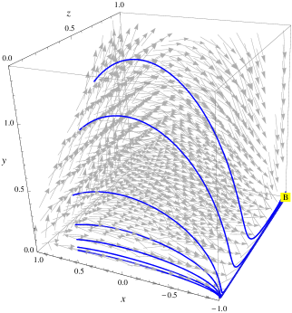
Figure 1: This plot represents a set of trajectories evolving in the three dimensional phase space $\left(x,\>y,\>z\right)\equiv\left(\dot{\phi},\>\kappa V/3H^{2},\>\rho/\rho_{\textrm{crit}}\right)$; also the complete vector field generated by the dynamical system is shown. All the possible trajectories are tangent to this vector field. The initial conditions for solving the dynamical system Eqs. (31)-(34) are chosen such that the trajectories start from locations near the $x-y$ plane. In this plane, $z\approx 0$, consequently $\rho\ll\rho_{\textrm{crit}}$. The different curves are obtained varying the initial value of the tachyon field $\phi_{0}$. Point B correspond to the location in the phase space where the semiclassical bounce is defined.

In figure 1 we show a selection of numerical solutions of the dynamical system Eqs. (31)–(34), in terms of the variables $\left(x,\>y,\>z,\>s\right)$. This figure represents trajectories which start from the lower $x-y$ plane and evolve in the phase space. These trajectories will initially converge to a point where $\dot{\phi}\rightarrow-1$, along the $x-y$ plane; however, in the vicinity of this point, they diverge along the $y-z$ plane and move away from it. This point can be identified to be the saddle fixed fixed points $P_{2}$ or $P_{8}$.

However, it is pertinent to point the following. Figure 1 involves parametric functions $x\left(N\right)$, $y\left(N\right)$ and $z\left(N\right)$. The numerical solution shows that the variable $N$ is only defined on a finite interval $\left[0,\>N_{{\rm bounce}}\right]$; this can be seen from Eq. (23) in which the scale factor is bounded from below, i.e., $a_{{\rm min}}<a<a_{0}$. In fact, and contrasting with the classical solution us:2013a , where $x\left(N\rightarrow\infty\right)\rightarrow\pm 1$ and $y\left(N\rightarrow\infty\right)\rightarrow 0$ are asymptotic limits, in the semiclassical scenario, the variable $N$ is bounded at the bounce. This boundary is shown in figure 1 where the curves end at a region where $z\rightarrow 1$ (identified as point B in the plot), which consequently, cannot be classified as a fixed point of the dynamical system. The numerical study supports the analytical discussion that the solutions in Ref. us:2013a for points $P_{1}$, $P_{2}$, $P_{7}$ and $P_{8}$, are now avoided on the semiclassical trajectories. In addition, for all the trajectories on the phase space shown in figure 1, point $B$ corresponds to a bouncing scenario which we will analyse it on the next section.

IV Semiclassical collapse end state

In this section we present additional results related to the numerical studies of Eqs. (8)–(21).

IV.1 Tracking solutions: Tachyon versus barotropic fluid

Figure 2: Behaviours of the scale factor $a(t)$ in the semiclassical (full line), and classical (dashed curve) regime. We considered the initial conditions as: $\rho_{0}=0.04$, $V_{0}=0.001$, $a(0)=2$, $\dot{\phi}\left(0\right)=0.5$ and $\phi_{0}=0.6$. We also have $\gamma=0.1$.

Figure 2 show the behaviour of the scale factor. Therein we observe that in the limit $\rho\rightarrow\rho_{\text{crit}}$, when the Hubble rate vanishes, the classical singularity is replaced by a bounce (cf. figure 2). In figure 3 we represent the energy densities, $\rho_{\gamma}(t)$ (left plot) and $\rho_{\phi}(t)$ (center plot), for different values of the barotropic parameter $\gamma$ at the bounce. We see that three scenarios have to be considered. When the energy densities of the tachyon and of the fluid scale exactly at the same power of the scale factor, namely

$$\rho_{\phi}\ \approx\ \rho_{\gamma}\ \approx\ \rho_{0}\,a^{-3\gamma},$$ (38)

then the semiclassical solutions display a tracking behaviour RLazkoz ; Liddle . Numerical analysis shows that this happens when the barotropic parameter is approximately $\gamma\sim 1$, that is, the collapse matter content acts like dust. From Eq. (38), we have $a_{\textrm{crit}}=\left[\rho_{\textrm{crit}}/\left(2\rho_{0}\right)\right]^{-1/3}$ at the bounce for the tracking solution. In the case where $\gamma>1$ the solution at the bounce is fluid dominated, whereas for $\gamma<1$, the tachyon field is the dominant component of the energy density content of the system; in the limit case where the barotropic fluid is absent (i.e. $\gamma=0$ and $\rho_{\gamma}=0$) the collapsing system is purely tachyonic. This solution will further enhance the characteristics of the tachyon dominated solutions.

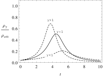
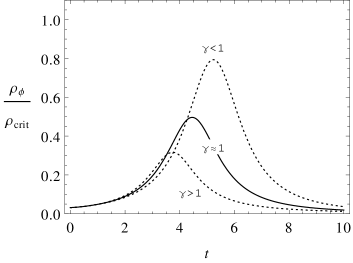
Figure 3: Behaviours of the energy densities $\rho_{\gamma}(t)$ (left plot) and $\rho_{\phi}(t)$ (right plot) for different values of the barotropic parameter $\gamma$. We have considered the same initial energy densities for the barotropic fluid and the tachyon field. At the bounce we have three different scenarios concerning the matter content dominance. When $\gamma\approx 1$ the system exhibits a tracking solution. If $\gamma>1$ the fluid is dominant, whereas for $\gamma<1$ it is the tachyon field that is dominant.

From figure 3 we also observe that, starting from very low values of the energy density (classical regime), a system that is fluid dominated reaches the bounce faster than a system that is tachyon dominated. This seems to point to the fact that a fluid dominant solution will drive the energy density until its critical value more efficiently than when the tachyon field is dominant. In the absence of the barotropic fluid, the matter content of the collapse is purely tachyonic, so the tachyon density $\rho_{\phi}$ will reach the critical value $\rho_{\rm crit}$ at the bounce. In this case, since there exist no barotropic fluid to push the collapse, the time required to reach the bounce will be maximized. In order to explain this result, let us consider what happens to the total pressure $p_{\phi}+p_{\gamma}$ for each solutions discussed in this section. When the tachyon field is dominant, for $\gamma<1$, the total pressure

$$p\ =\ -V(\phi)\sqrt{1-\dot{\phi}^{2}}+\left(\gamma-1\right)\rho_{\gamma}\ ,$$ (39)

is negative until the collapsing body reaches the bounce. In fact, near the bounce $\dot{\phi}\rightarrow 1$ and eq. (39) becomes $p\thickapprox\left(\gamma-1\right)\rho_{\gamma}<0$. For the tracking solution $\left(\gamma\sim 1\right)$, we have $p\sim 0$ and the matter content behaves as dust. Finally, for the fluid dominated solutions, the total pressure is approximately $p\thickapprox\left(\gamma-1\right)\rho_{\gamma}$, which is positive because in this case $\gamma>1$. Consequently, in this last scenario, the positive pressure drives the fluid dominant content of the energy density rapidly towards its critical value, $\rho_{\text{crit}}$, at the semiclassical bounce.

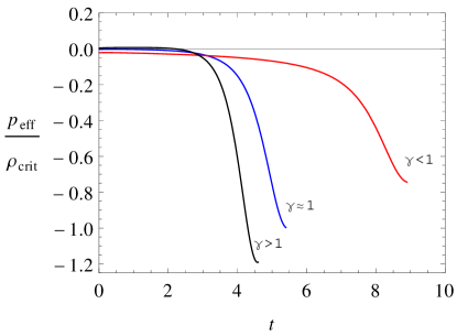
Figure 4: In this plot we represent the evolution of the effective pressure $p_{\rm eff}$, for the three cases $\gamma>1$, $\gamma\approx 1$ and $\gamma<1$ until the bounce is reached.

In addition, when we consider Eq. (10) for the effective pressure, in particular its value at the bounce (where $\rho\rightarrow\rho_{\textrm{crit}}$),

$$\begin{cases}p_{\textrm{eff}}^{\phi}\ \approx\ -\left(\gamma-1\right)\rho_{\gamma}-\rho_{\textrm{crit}}\ ,&\quad\quad\gamma<1\\ p_{\textrm{eff}}^{tr}\ \approx\ -\rho_{\textrm{crit}}\ ,&\quad\quad\gamma\approx 1\\ p_{\textrm{eff}}^{\gamma}\ \approx\ -\left(\gamma-1\right)\rho_{\gamma}-\rho_{\textrm{crit}}\ ,&\quad\quad\gamma>1\end{cases}$$ (40)

we can establish that $p_{\textrm{eff}}^{\gamma}<p_{\textrm{eff}}^{tr}<p_{\textrm{eff}}^{\phi}<0$ (see figure 4). In this plot we have that for the fluid dominated solution, the effective pressure start at a positive value (pushing the density of collapsing system to increase rapidly towards its critical value $\rho\rightarrow\rho_{\text{crit}}$). However, near the bounce, the effective pressure rapidly switches to negative values. In contrast, for the tachyon dominated solution, the effective pressure starts from negative values from the beginning; this is related to the fact that the initial energy densities of both the tachyon and barotropic fluid are approximate. Moreover, the change near the bounce is less pronounced in this last case. Therefore the evolution of the collapse is slower and the bounce is delayed when compared to the fluid dominated scenario. It is straightforward to verify that the tracking solution provides an intermediate context between the fluid and tachyon dominated solutions.

IV.2 Horizon formation

From the equation $\dot{R}^{2}(t,r_{b})=1$ (where $r_{b}$ is the radius of the boundary shell) we can determine the speed of the collapse, $|\dot{a}|_{\mathrm{AH}}$, at which horizons form, i.e., $|\dot{a}|_{\mathrm{AH}}=\frac{1}{r_{b}}$. When the speed of collapse, $|\dot{a}|$, reaches the value $1/r_{b}$, then an apparent horizon forms. Thus, if the maximum speed $|\dot{a}|_{\text{max}}$ is lower than the critical speed $|\dot{a}|_{\mathrm{AH}}$, no horizon can form. More precisely, in order to discuss the dynamics of the trapped region in the perspective of the effective dynamics scenario, we consider $|\dot{a}|$ from Eq. (6) to be equal to $|\dot{a}|_{\mathrm{AH}}=1/r_{b}$. Solving this new equation for $\rho$ and $a$ we get scale factors and energy densities at which the horizon forms. Figure 5 represents the speed of the collapse, $|\dot{a}|$, as a function of the scale factor, reaching the maximum value $|\dot{a}|_{\textrm{max}}$.

The tachyon field equation (21) implies that $\phi\equiv\phi\left(a\right)$. Therefore, from Eqs. (16)–(18) we can also establish that the total energy density can be expressed as a function $\rho\equiv\rho\left(a\right)$. Then, we can rewrite $|\dot{a}|=\frac{1}{r_{b}}$ by setting $X:=\rho/\rho_{{\rm crit}}$ and $a^{2}:=f(X)$ as

$$f\left(X\right)X\left(1-X\right)-A=0\ ,$$ (41)

where $A:=3/\left(8\pi G\rho_{{\rm crit}}r_{b}^{2}\right)$ is a constant. The study of roots of the Eq. (41) enables us to get the values of energy density at which an apparent horizons form. Considering more closely Eq. (41), we need to estimate the behaviour of the function $f(X)$. In figures 2 and 3, we have that $f(X)$ is minimum when $X$ is maximum. It is also expected that, since $f(X)$ is a monotonically decreasing function near the bounce, Eq. (41) is essentially described as a second order polynomial. Therefore, depending on the initial conditions, in particular on the choice of the $r_{b}$, three cases can be evaluated, which correspond to no apparent horizon formation ($A/f\left(X\right)>1/4$), one and two horizons formation ($A/f\left(X\right)\leq 1/4$).

Let us introduce a radius $r_{\star}$, defined by

$$r_{\star}\ :=\ \frac{1}{|\dot{a}|_{\text{max}}}\ .$$ (42)

We see that $r_{\star}$ determines a threshold radius for the horizon formation; if $r_{b}<r_{\star}$, then no horizon can form at any stage of the collapse. The case $r_{b}=r_{\star}$ corresponds to the formation of a dynamical horizon at the boundary of the two space-time regions dynHorizon . Finally, for the case $r_{b}>r_{\star}$ two horizons will form, one inside and the other outside of the collapsing matter.

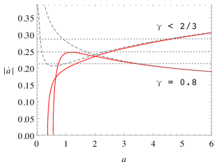
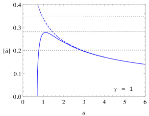
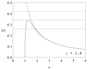
Figure 5: The speed of collapse, $|\dot{a}|$, with respect to the scale factor $a$, in the semiclassical (full line), and classical (dashed curve) regime. We considered the initial conditions as: $\rho_{0}=0.04$, $V_{0}=0.001$, $a(0)=2$, $\dot{\phi}\left(0\right)=0.5$ and $\phi_{0}=0.6$. Top left panel is for a tachyon dominated solution with $\gamma=0.8$ and $\gamma<2/3$. The top right panel is for a tracking solution with $\gamma=1$. Finally, the lower center panel is for a fluid dominated solution with $\gamma=1.5$ The dotted lines are for the different values of $r_{b}<r_{\star}$ (upper line), $r_{b}=r_{\star}$ (inner line) and $r_{b}>r_{\star}$ (lower line).

The behaviour of the three possible scenarios (tracking solution, tachyon and fluid dominated solutions) are also represented in figure 5. We note that only one horizon forms for some particular tachyon dominated solutions. Therefore, for these solutions the bounce will be covered by an horizon. In order to further clarify this aspect, we note that when more than one horizon forms, the speed of the collapse $\dot{a}$ must have a local maximum. In that case, the acceleration must be $\ddot{a}=0$, and from equations (6)–(8) we can determine that this local maximum can be found by imposing

$$\frac{\ddot{a}}{a}\ =\ \dot{H}+H^{2}\ =\ -\frac{\kappa}{6}\left(\rho_{\rm crit}+3p_{\rm crit}\right)\ =\ 0\ .$$ (43)

This last condition, being equivalent to $\rho_{\textrm{eff}}=-3\,p_{\textrm{eff}}$, must be closely monitored for the three different solutions discussed in this section. For the fluid dominated solution, and since the effective pressure starts from positive values and evolve to negatives one near the bounce, it is straightforward to verify that the function $-3\,p_{\textrm{eff}}$ must intersect $\rho_{\textrm{eff}}$ at some point before reaching the bounce. For the tracking solution we can use the same argument but with an initial effective pressure starting near zero and reaching $3\,\rho_{\textrm{crit}}$ at the bounce. Finally, the case of the tachyon dominated solution depends on the value of the barotropic parameter $\gamma$. When the initial values for the effective pressure and energy densities are $p_{\textrm{eff}}^{\phi}\approx-\left(\gamma-1\right)\rho_{\gamma 0}$ and $\rho_{\textrm{eff}}^{\phi}\approx\rho_{\gamma 0}>\rho_{\phi 0}$, respectively; then, if $\gamma>2/3$, the argument given for the tracking and fluid dominated solution is also valid for this case. However, if $\gamma<2/3$, there will be at the most one horizon forming. Besides taking $\gamma>2/3$, if we consider an unbalanced initial energy density, with the tachyon being slightly dominant, i.e., $\rho_{\phi 0}\geq\rho_{\gamma 0}$, a local maximum for $\dot{a}$ will also be present.

IV.3 Exterior geometry

Finally, the discussion of the final outcomes related to the semiclassical solutions follows the one made in Ref. us:2013c . In this previous work, it is described that the fate of the collapsing star (with a massless scalar field as matter source) whose shell radius is less than the threshold radius $r_{\star}$ points to the existence of an energy flux radiated away from the interior space-time and reaching the distant observer. In the present study, for a collapsing system whose initial boundary radius $r_{b}$ is less than $r_{\star}$, we analyze the resulting mass loss due to the semiclassical modified interior geometry. In particular, this analysis is only carried for the tracking solution or fluid dominated scenario, since the tachyon dominated solution develops no more than one horizon, for $\gamma<2/3$ and $\rho_{\gamma 0}\geq\rho_{\phi 0}$, before reaching the bounce. Let us designate the initial mass function at scales $\rho\ll\rho_{{\rm crit}}$, i.e, in the classical regime, as $F_{0}=(8\pi G/3)\rho_{0}R_{0}^{3}$, with $\rho_{0}=\rho_{\phi 0}+\rho_{\gamma 0}$. For $\rho\lesssim\rho_{{\rm crit}}$ (in the semiclassical regime) we have, instead, an effective mass function $F_{\text{eff}}$ given by Eq. (13). Then, the (quantum geometrical) mass loss, $\Delta F/F_{0}$ (where $\Delta F=F_{0}-F_{\text{eff}}$), for any shell, is provided by the following expression:

$$\frac{\triangle F}{F(a_{0})}\ =\ 1-\frac{F_{\text{eff}}}{F_{0}}\ =\ 1-\sqrt{\frac{\rho}{\rho_{0}}}\left(1-\frac{\rho}{\rho_{{\rm cr}it}}\right)\ .$$ (44)

As $\rho$ increases the mass loss decreases positively until it vanishes at a point. Then, $\Delta F/F$ continues decreasing (negatively) until it reaches to a minimum at $\rho=\rho_{{\rm crit}}/3$. Henceforth, in the energy interval $\rho_{{\rm crit}}/3<\rho<\rho_{{\rm crit}}$, the mass loss increases until the bouncing point at $\rho\rightarrow\rho_{\text{crit}}$, where $\Delta F/F\rightarrow 1$; this means that the quantum gravity corrections, applied to the interior region, give rise to an outward flux of energy near the bounce in the semiclassical regime. The previously described behaviour for the mass loss will be qualitatively identical with respect to the solution considered. Therefore the tachyon (when $\gamma>2/3$ or the initial energy densities are $\rho_{\phi 0}>\rho_{\gamma 0}$), fluid dominated or tracking solutions will exhibit the same profile for the mass loss. The only difference between these three cases, shown in the right plot of figure 6, is the value of the radius where the mass loss reaches the maximum $\Delta F/F\rightarrow 1$. In the last section we discussed the fact that the bounce occurring in the tachyon dominated solution is delayed compared with the other solutions. Consequently, the bounce (where $\Delta F/F\rightarrow 1$) take place for a smaller value of the radius $R$.

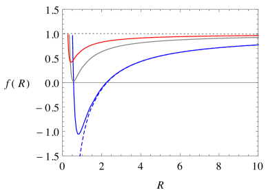
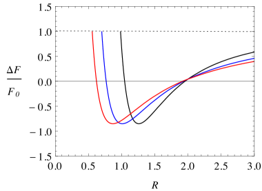
Figure 6: The left plot represents the tracking solution ($\gamma\approx 1$) boundary function, $f(R)$, with respect to the radius $R$, in the semiclassical (full line), and classical (dashed curve) regime. We considered the initial conditions as: $\rho_{0}=0.04$, $V_{0}=0.001$, $a(0)=2$, $\dot{\phi}\left(0\right)=0.5$ and $\phi_{0}=0.6$. The right plot shows the behaviour of the mass loss $\Delta F/F$, as a function of area radius $R$. In this last plot we present the behaviour of the tachyon dominated solution (reaching $\Delta F/F\rightarrow 1$ at the smaller $R$), the tracking solution (reaching $\Delta F/F\rightarrow 1$ at the intermediate $R$) and the fluid dominated solution (reaching $\Delta F/F\rightarrow 1$ at the bigger $R$).

In the other case, where $r_{b}\geq r_{\star}$, in which one or two horizon form, the exterior geometry can be obtained by matching the interior to a generalized Vaidya exterior geometry at the boundary $r_{b}$ of the cloud. Following the method provided in Ref. us:2013a , we can write the exterior metric in advanced null coordinates $(v,R)$ as

$$ds_{{\rm(ext)}}^{2}\ =\ -f(R,v)dv^{2}-2dvdR+R^{2}d\Omega^{2}\ ,$$ (45)

where the exterior function is given by $f(v,R)=1-2Gm(v,R)/R$. By applying the matching conditions at the boundary $r_{b}$ we have that

$$m(v,R)\ =\ M-\frac{3}{4\pi\rho_{{\rm crit}}}\frac{M^{2}}{R^{3}}$$ (46)

where we have defined $M:=(4\pi/3)\rho R^{3}$ is the mass within the volume $R^{3}$. For a fluid dominated solution we have

$$M\ \approx\ \frac{4\pi}{3}\rho_{0}R_{0}^{3\gamma}R^{-3(\gamma-1)}\ .$$ (47)

In the limit case $\gamma\sim 1$, i.e. the tracking solution, Eq. (47) reduces to

$$M\ =\ M_{0}\ =\ \left(4\pi/3\right)\rho_{0}R_{0}^{3}\ ,$$ (48)

which presents a modified Oppenheimer-Snyder collapse Oppenheimer of homogeneous dust matter. Figure 6 shows the numerical behaviour of the boundary function $f(R)$ in the classical (dashed curve) and semiclassical regime (solid curves) for the cases of the initial radius $r_{b}<r_{\star}$ and $r_{b}\geq r_{\star}$. The later shows the behaviour of an exotic non-singular black hole geometry which is different from its classical counterpart. Similarly, for a tachyon dominated case with $\gamma<1$ (or a purely tachyonic collapse), the mass $M\approx\left(4\pi/3\right)\rho_{\phi}R^{3}$ reads

$$M(\phi)\ \approx\ \frac{4\pi R^{3}}{3}\frac{V(\phi)}{\sqrt{1-\dot{\phi}^{2}}}\ .$$ (49)

It should be noticed that the energy density $\rho_{\phi}$ is upper bounded by the critical density $\rho_{\rm crit}$, thus, the mass $M$ is always finite.

V Conclusion and discussion

In this paper we employed an effective scenario imported from LQG, namely the “holonomy” corrections to the dynamics of the gravitational collapse whose matter content involves a self interacting tachyon field and a barotropic fluid. Our aim was to enlarge the discussion on tachyon field gravitational collapse. More concretely, on the one hand, extending the scope analyzed in Ref. us:2013a , by investigating how the quantum gravity correction term $-\rho^{2}/\rho_{{\rm crit}}$, can alter the fate of the collapse. Using a dynamical system analysis, we subsequently found a class of solutions. Our semiclassical analysis showed that, the corresponding stable fixed point (attractor) solutions in the classical general relativistic collapse become saddle points in our semiclassical collapse; hence, the classical black hole and naked singularities produced in Ref. us:2013a are no longer present within the loop semiclassical regime studied in this paper. We found conditions to define a tachyon or fluid dominated regimes close to the bounce, depending on the value of the barotropic parameter of the fluid. The transition from one regime to the other shows the emergence of a tracking solution where the collapsing matter behaves as dust. It was also observed that, in scenarios with similar initial conditions, a fluid dominated solution drives the energy density of the collapsing cloud until the critical value $\rho_{\rm crit}$ more rapidly than a tachyon dominated solution.

Our analysis provides elements to contrast the correction features of holonomy to those given by inverse triad modification us:2013b , as far as tachyon scalar field gravitational collapse is concerned. Nevertheless, the issue of inverse triad effects is quite subtle in LQC; it has been shown that for space-times with non-compact topology they can not be consistently incorporated. (We suggest the reader to see Refs. (LQC-AS, ; Rev1, ; Rev2, ) where further technical details on the problem with inverse scale factor effects is discussed.) In addition, it is important to mention that for space-times with spatial curvature there is no problem in including inverse scale factor effects (see Ref. Rev3 ). In the aforementioned case of a gravitational collapse modified by inverse triad corrections, the energy density of collapsing matter source is a decreasing function of time towards the star center and remains constant there us:2013b . However, in the presence of the holonomy corrections, the quadratic density modifications provide an upper limit $\rho_{{\rm crit}}$ for the energy density $\rho$ of the collapsing matter, indicating that the herein semiclassical collapse leads to a non-singular bounce at the critical density $\rho=\rho_{{\rm crit}}$. The mass loss obtained by the inverse triad scenario us:2013b , was characterised by the reduction of energy density and mass function towards the star center, which leads to an outward energy flux. However, in the present semiclassical model, for a particular range of the radius of the boundary shell (i.e., $r_{b}<r_{\star}$), the energy density and the mass function growth of the collapsing cloud is followed by the effective mass loss reduction near the bounce, which subsequently gives rise to an outward energy flux at the collapse end state. In addition, a detailed dynamical system analysis in the inverse triad scenario predicted only one stable solution which allowed a barotropic fluid with a parameter satisfying the range $8/5\leq\gamma<2$ (where the superior limit is a consequence of the energy conditions imposed in the classical setting, discussed in Ref. us:2013a ). In contrast to the case studied in Ref. us:2013b , the barotropic fluid parameter is less constrained and solutions with $0<\gamma<2$, as predicted by the classical model, are allowed to evolve until the bounce.

We further investigated, by means of numerical studies, the evolution of trapped surfaces during the collapse in order to determine its final state. We found a threshold radius for the collapsing matter cloud in order to form a black hole at late time stages. The physical modifications related to the semiclassical regime provided three cases for the trapped surfaces formation, depending on the initial conditions of the collapsing star. In particular, our solutions showed that, if the initial boundary radius of the collapsing cloud is less than a threshold radius, namely $r_{\star}$, no horizon forms during the collapse, whereas for the radius equal and larger than the $r_{\star}$, one and two horizons form, respectively. It is worthy to mention that, for the tachyon dominated solutions, the previous scenario only happens when the barotropic parameter is $\gamma>2/3$ or the initial energy densities satisfy $\rho_{\phi 0}\geq\rho_{\gamma 0}$. When $\gamma<2/3$ and $\rho_{\phi 0}<\rho_{\gamma 0}$, not more than one apparent horizon forms.

Our effective scenario, in the presence of a tachyon field joined to a barotropic fluid, share a few common features to the one where, instead, a homogeneous massless scalar field was considered for the collapsing matter content us:2013c . In both contexts, and in the particular case in which no horizon forms, it is shown that, as the collapse evolves, the energy density increases towards a maximum value $\rho_{\textrm{crit}}$ at the bounce. Moreover, in these semiclassical scenarios, the effective energy density reduction leads to a positive mass loss near the bounce. This results in a positive luminosity near the bounce which gives rise to an outward energy flux from the interior region, that may reach to a distant observer. In addition, in the cases in which one or two horizons form, the resulting exterior geometry corresponds to exotic non-singular black holes which are different from the Schwarzschild one (see also Refs. (Bojowald:2005, ; VHussain, ) for such a black hole formation).

In our collapsing system, additional physical situations might arise from the interplay between the tachyon and the barotropic fluid. Namely, the distinct matter dominance regimes yield a wider variety of outcomes, either for the horizon formation, or when the efficiency to reach the semiclassical bounce is concerned. Including an interaction term $\Gamma_{{\rm int}}$, that could account for a transfer of energy between the tachyon field and the barotropic fluid, is expected to change the results presented here. In fact, it is reasonable to anticipate that the conditions required to define the fluid or tachyon dominated regimes will certainly be less simple. The emergence of these regimes will certainly reflect more than just the variation of the barotropic parameter. Another interesting question to be addressed, in this context, is related to the existence of a tracking behaviour and under which conditions it becomes possible. In fact, from the results presented here, the emergence of a tracking behaviour seems to occur at the transition between the fluid and the tachyon dominated regimes. Would this situation be maintained in the interacting case? The answers to these questions will also have an impact on the discussion about the horizon formation, since it is closely related to the matter dominance present at the bounce. Therefore, one interesting extension to this work will be to consider an interaction between the tachyon and the barotropic fluid.

The qualitative picture depicted from our toy model is strongly dependent on the choice of a homogeneous interior space-time. Nevertheless, in a realistic collapsing scenario one should employ a more general inhomogeneous setting (see Refs. (Bojowald:2006, ; Campiglia:2007, ), where a detailed introduction to recent techniques to handle inhomogeneous systems provides the ingredients on how to extend the limited homogeneous case). When we apply homogeneous techniques, the quantum effects are restricted to the interior space-time, whereas, the outer space-time region is assumed to be a generalised Vaidya metric defined by classical general relativity. Some imprint of the interior quantum effects are transported to the outside, by imposing suitable matching conditions at the boundary surface, where it enters the Vaidya solution effectively through a nonstandard energy-momentum tensor. This procedure is also restricted by the fact that a full inhomogeneous quantization, also covering the exterior region, is expected to provide significant modifications to the space-time structure. However, some indications on how the matter content might affect the bounce scenario may still be valid in a more general inhomogeneous setting.

VI Acknowledgments

Y.T. was supported by FCT (Portugal) through the fellowship SFRH/BD/43709/2008 and a grant from CNPq (Brazil). This research work was supported by the grants CERN/FP/123609/2011 and CERN/FP/123618/2011 and PEst-OE/MAT/UI0212/2014.

References

- (1) P. Joshi, Gravitational Collapse and Space-Time Singularities, (Cambridge University Press, England, 2007).
- (2) R. Penrose, Phys. Rev. Lett. 14, 57 (1965); S. W. Hawking, Proc. R. Soc. A 300, 187 (1967); S. W. Hawking and R. Penrose, Proc. R. Soc. A 314, 529 (1970).
- (3) S. W. Hawking and G. F. R. Ellis, The Large Scale Structure of Space-Time, (Cambridge University Press, England 1974).
- (4) A. Ashtekar and J. Lewandowski, Class. Quantum Grav. 21, R53 (2004); T. Thiemann, Introduction to Modern Canonical Quantum General Relativity (Cambridge University Press, Cambridge, England, 2007).
- (5) A. Ashtekar, M. Bojowald and J. Lewandowski, Adv. Theor. Math. Phys. 7, 233 (2003).
- (6) A. Ashtekar and P. Singh, Loop quantum cosmology: a status report, Class. Quantum Grav. 28, 213001 (2011).
- (7) M. Bojowald, Canonical Gravity and Applications: Cosmology, Black Holes, and Quantum Gravity (Cambridge University Press, Cambridge, England, 2010).
- (8) M. Bojowald, R. Goswami, R. Maartens, and P. Singh, Phys. Rev. Lett. 95, 091302 (2005).
- (9) R. Goswami, P. S. Joshi and P. Singh, Phys. Rev. Lett. 96, 031302 (2006).
- (10) A. Ashtekar, T. Pawlowski and P. Singh, Phys. Rev. Lett. 96, 141301 (2006).
- (11) Y. Tavakoli, J. Marto and A. Dapor, Int. J. Mod. Phys. D 27, No. 7, 1450061 (2014).
- (12) C. Bambi, D. Malafarina and L. Modesto, Phys. Rev. D 88, 044009 (2013).
- (13) Y. Tavakoli, J. Marto, A. Hadi Ziaie and P. Vargas Moniz, Gen. Rel. Grav. 45, 819 (2013).
- (14) L.-F. Li and J.-Y. Zhu, Phys. Rev. D 79, 124011 (2009).
- (15) Y. Tavakoli, J. Marto, A. H. Ziaie and P. V. Moniz, Phys. Rev. D 87, 024042 (2013).
- (16) V. Taveras, IGPG preprint (2006).
- (17) R. Herrera, D. Pavón and W. Zimdahl, Gen. Rel. Grav. 36, 9 (2004).
- (18) W. Chakraborty and U. Debnath, Astrophys. and Space Science 315, 167 (2008).
- (19) M. R. Setare, J. Sadeghi and A. R. Amani, Phys. Lett. B 673, 4 (2009).
- (20) H. K. Khalil, Nonlinear Systems, 2nd edition (Englewood Cliffs. NJ: Prentice Hall, 1996) pp 167-177.
- (21) Juan M. Aguirregabiria and Ruth Lazkoz, Phys. Rev. D 69, 123502 (2004).
- (22) A. R. Liddle and R. J. Scherrer, Phys. Rev. D 59, 023509 (1998).
- (23) S. A. Hayward, Phys. Rev. D 49, 6467 (1994); A. Ashtekar and B. Krishnan, Phys. Rev. Lett. 89, 261101 (2002).
- (24) Benjamin K. Tippett and Viqar Husain, Phys. Rev. D 84, 104031 (2011).
- (25) M. Bojowald, R. Swiderski, Class. Quantum Grav. 23, 2129 (2006).
- (26) M. Campiglia, R. Gambini and J. Pullin, Class. Quantum Grav. 24, 3649 (2007).
- (27) J. R. Oppenheimer and H. Snyder, Phys. Rev. 56, 455 (1939).
- (28) A. Ashtekar, T. Pawlowski and P. Singh, Phys. Rev. D 74, 084003 (2006).
- (29) A. Ashtekar, T. Pawlowski, P. Singh and K. Vandersloot, Phys. Rev. D 75, 024035 (2007).
- (30) B. Gupt and P. Singh, Phys. Rev. D 85, 044011 (2012).