Viscoelastic Tidal Dissipation in Giant Planets and Formation of Hot Jupiters Through High-Eccentricity Migration

Abstract

We study the possibility of tidal dissipation in the solid cores of giant planets and its implication for the formation of hot Jupiters through high-eccentricity migration. We present a general framework by which the tidal evolution of planetary systems can be computed for any form of tidal dissipation, characterized by the imaginary part of the complex tidal Love number, ${\rm Im}[{\tilde{k}}_{2}(\omega)]$, as a function of the forcing frequency $\omega$. Using the simplest viscoelastic dissipation model (the Maxwell model) for the rocky core and including the effect of a nondissipative fluid envelope, we show that with reasonable (but uncertain) physical parameters for the core (size, viscosity and shear modulus), tidal dissipation in the core can accommodate the tidal-Q constraint of the Solar system gas giants and at the same time allows exoplanetary hot Jupiters to form via tidal circularization in the high-e migration scenario. By contrast, the often-used weak friction theory of equilibrium tide would lead to a discrepancy between the Solar system constraint and the amount of dissipation necessary for high-e migration. We also show that tidal heating in the rocky core can lead to modest radius inflation of the planets, particularly when the planets are in the high-eccentricity phase ($e\sim 0.6$) during their high-e migration. Finally, as an interesting by-product of our study, we note that for a generic tidal response function ${\rm Im}[{\tilde{k}}_{2}(\omega)]$, it is possible that spin equilibrium (zero torque) can be achieved for multiple spin frequencies (at a given $e$), and the actual pseudosynchronized spin rate depends on the evolutionary history of the system.

1 Introduction

In recent years, high-eccentricity migration has emerged as one of the dominant mechanisms responsible for the formation of hot Jupiters. In this mechanism, a gas giant which is formed beyond the snow line is first excited into a state of very high eccentricity ($e\mathrel{\raise 1.29167pt\hbox{$>$}\mkern-14.0mu\lower 2.58334pt\hbox{$\sim$}}0.9$) by few-body interactions, either via dynamical planet-planet scatterings (Rasio & Ford 1996; Weidenschilling & Marzari 1996; Zhou, Lin & Sun 2007; Chatterjee et al. 2008; Juric & Tremaine 2008) or/and secular interactions between multiple planets, or the Kozai effect induced by a distant companion (Wu & Murray 2003; Fabrycky & Tremaine 2007; Wu, Murray & Ramshhai 2007; Nagasawa, Ida & Bessho 2008; Katz, Dong & Malhotra 2011; Naoz et al. 2011,2013; Wu & Lithwick 2011; Naoz, Farr & Rasio 2012; see also Dawson & Murray-Clay 2013). Due to the high eccentricity, the planet passes quite close to its host star at periastron, and tidal dissipation in the planet extracts energy from the orbit, leading to inward migration and circularization of the planet’s orbit.

Tidal effects on the orbital evolution of binaries are often discussed using the weak friction theory of equilibrium tides (Darwin 1879; Alexander 1973; Hut 1981; Eggleton et al. 1998), according to which the rate of decay of the semi-major axis ($a$) for a pseudosynchronized planet can be written as

$$\left|{\dot{a}\over a}\right|=6k_{2}\tau\left({GM_{\star}\over a_{F}^{3}}\right)\left({R_{\mathrm{p}}\over a_{F}}\right)^{5}{M_{\star}\over M_{\mathrm{p}}}\sqrt{a_{F}\over a}\,F(e).$$ (1)

Here, $M_{\mathrm{p}}$ and $R_{\mathrm{p}}$ are the mass and radius of the planet, $M_{\star}$ is the mass of the central star, $a_{F}\equiv a(1-e^{2})$ is the final circularization radius (assuming orbital angular momentum conservation), $k_{2}$ the tidal Love number, $\tau$ is the tidal lag time (assumed constant in the weak friction theory), and $F(e)$ is a function of eccentricity of order $(1-10)$ and given by $F(e)=f_{1}(e)-f_{2}^{2}(e)/f_{5}(e)$, where $f_{1}$, $f_{2}$ and $f_{5}$ are given by Eq. (11) of Hut (1981). By requiring that the high-e migration happens on a timescale less than $10$ Gyr we can place a constraint on $\tau$:

$$\left({GM_{\star}\over a^{3}_{F}}\right)^{1/2}\tau\mathrel{\hbox{\hbox to0.0pt{\hbox{\lower 3.0pt\hbox{$\sim$}}\hss}\hbox{\raise 2.0pt\hbox{$>$}}}}3\times 10^{-5}\left({a\over 5\textrm{AU}}\right)^{1/2}\left({a_{F}\over 0.06\textrm{AU}}\right)^{6}$$

$$\qquad\times\left({M_{\star}\over M_{\sun}}\right)^{-3/2}{M_{\mathrm{p}}\over M_{J}}\left({R_{\mathrm{p}}\over R_{J}}\right)^{-5}\left({k_{2}\over 0.38}\right)^{-1}.$$ (2)

Note that instead of $\tau$, tidal dissipation is often parametrized by the tidal quality factor $Q\equiv(\tau\omega)^{-1}$, where $\omega$ is the tidal forcing frequency. Thus, the above constraint on $\tau$ translates to $Q\mathrel{\raise 1.29167pt\hbox{$<$}\mkern-14.0mu\lower 2.58334pt\hbox{$\sim$}}3\times 10^{4}$ at $\omega\sim(GM_{\star}/a_{F}^{3})^{1/2}\sim 2\pi/(5~{}{\rm d})$ [for the canonical parameters adopted in Eq. (2)]. A similar constraint can be obtained by integration over the planets’ orbital evolution (e.g., Fabrycky & Tremaine 2007; Leconte et al. 2010; Matsumura, Peale & Rasio 2010; Hansen 2012; Naoz et al. 2012; Socrates, Katz & Dong 2012b).

The tidal $Q$ for Solar system giant planets can be measured or constrained by the tidal evolution of their satellites (Goldreich & Soter 1966). For Jupiter, Yoder & Peale (1981) derived a bound $2\times 10^{-7}<k_{2}/Q_{J}<6\times 10^{-6}$ based on Io’s long-term orbital evolution (particularly the eccentricity equilibrium), with the upper limit following from the limited expansion of satellite orbits. Recent analysis of the astrometric data of Galilean moons gave $k_{2}/Q_{J}=(1.1\pm 0.2)\times 10^{-5}$ for the current Jupiter-Io system (Lainey et al. 2009), corresponding to $Q_{J}\simeq 3.5\times 10^{4}$ for the conventional value of the Love number $k_{2}=0.38$ (Gavrilov & Zharkov 1977). With Jupiter’s spin period 9.9 hrs and Io’s orbital period 42.5 hrs, the tidal forcing frequency on Jupiter from Io is $\omega=2\pi/(6.5~{}{\rm hr})$, and the tidal lag time is then $\tau_{J}=(Q_{J}\omega)^{-1}\simeq 0.1$ s.

For Saturn, theoretical considerations based on the long-term evolution of Mimas and other main moons (with the assumption that they formed above the synchronous orbit 4.5 Gyr ago) lead to the constraint $3\times 10^{-6}<k_{2}/Q_{S}<2\times 10^{-5}$ (Sinclair 1983; Peale 1999). However, using astrometric data spanning more than a century, Lainey et al. (2012) found a much larger $k_{2}/Q_{S}=(2.3\pm 0.7)\times 10^{-4}$, corresponding to $Q_{S}=(1-2)\times 10^{3}$ for $k_{2}=0.34$; they also found that $Q_{S}$ depends weakly on the tidal period in the range between $2\pi/\omega=5.8$ hrs (Rhea) and $7.8$ hrs (Enceladus).

Assuming that extra-solar giant planets are close analogs of our own gas giants, we can ask whether the aforementioned empirical constraints on $k_{2}/Q$ for Jupiter and Saturn are compatible with the extra-solar constraint [see Eq. (2)]. The difference between the two sets of constraints is the tidal forcing frequencies: For example, the Jupiter-Io constraint involves a single frequency ($P=6.5$ hrs), while high-e migration involves tidal potentials of many harmonics, all of them with periods longer than a few days. Socrates et al. (2012b) showed that the two sets of constraints are incompatible with the weak friction theory (see also Naoz et al. 2012): In order for hot Jupiters to undergo high-e migration within the age of their host stars, their required tidal lag times must be more than an order of magnitude larger than the Jupiter-Io constraint.

Tidal dissipation in giant planets is complex, and depends strongly on the internal structure of the planet, such as the stratification of the liquid envelope and the presence and properties of a solid core. There have been some attempts to understand the physics of tidal $Q$ in giant planets (see Ogilvie & Lin 2004 for a review). It has long been known (Goldreich & Nicholson 1977) that simple turbulent viscosity in the fluid envelopes of giant planets is many orders of magnitude lower than required by observations. Ioannou & Lindzen (1993a,b) considered a prescribed model of Jupiter where the envelope is not fully convective (contrary to the conventional model where the envelope is neutrally buoyant to a high degree; see Guillot 2005) and showed that the excitation and radiative damping of gravity waves in the envelope provide efficient tidal dissipation only at specific “resonant” frequencies. Lubow et al. (1997) examined similar gravity wave excitations in the radiative layer above the convective envelope of hot Jupiters. So far the most sophisticated study of dynamical tides in giant planets is that by Ogilvie & Lin (2004) (see also Goodman & Lackner 2009; Ogilvie 2009,2013), who focused on the tidal forcing of inertial waves (short-wavelength disturbances restored primarily by Coriolis force) in the convective envelope of a rotating planet [see Ivanov & Papaloizou (2007) and Papaloizou & Ivanov (2010) for highly eccentric orbits, and Wu (2005) for a different approach]. They showed that because of the rocky core, the excited inertial waves are concentrated on a web of “rays”, leading to tidal dissipation which depends on the forcing frequency in a highly erratic way. The tidal $Q$ obtained is typically of order $10^{6-7}$. It remains unclear whether this mechanism can provide sufficient tidal dissipation compared to the observational constraints.

The possibility of core dissipation in giant planets was first considered by Dermott (1979) but has not received much attention since. Recently, Remus et al. (2012a) showed that dissipation in the solid core could in principle satisfy the constraints on tidal $Q$ obtained by Lainey et al. (2009) for Jupiter and by Lainey et al. (2012) for Saturn.

In this paper, we continue the study of tidal dissipation in the solid core of giant planets and examine its consequences for the high-e migration scenario and for the thermal evolution of hot Jupiters. In section 2 we present the general tidal theory which may be used with any tidal response model. In section 3 we discuss a simple viscoelastic tidal response model and its range of applicability. In section 4 we use the general theory of section 2 in conjunction with the model of section 3 to compute high-e migration timescales and compare with the weak friction theory. We also examine the effect of tidal heating in the core for the radius evolution of the planets. We summarize our findings and conclude in section 5.

2 Evolution of Eccentric Systems with General Tidal Responses

Here we formulate the tidal evolution equations for eccentric binary systems. These equations can be applied to any tidal response model, where the complex Love number (defined below) is an arbitrary function of the tidal forcing frequency [see also Efroimsky & Makarov (2013), Mathis & Le Poncin-Lafitte (2009) and Remus et al. (2012a) for similar formalisms]. This formulation is valid as long as the responses of the body to different tidal components are independent of each other.

We consider a planet of mass $M_{\mathrm{p}}$, radius $R_{\mathrm{p}}$ and rotation rate $\Omega_{s}$ (assumed to be aligned with the orbital angular momentum axis), moving around a star (mass $M_{\star}$) in an eccentric orbit with semi-major axis $a$ and mean motion frequency $\Omega$. The tidal potential exerted on the planet by the star is given by

$$U({\bf r},t)=-GM_{\star}\sum_{m}{W_{2m}r^{2}\over D(t)^{3}}e^{-im\Phi(t)}Y_{2m}(\theta,\phi),$$ (3)

where $(r,\theta,\phi)$ is the position vector (in spherical coordinates) relative to the center of mass of the planet, $D(t)$ and $\Phi(t)$ are the time-dependent separation and phase of the orbit, and $m=0,\pm 2$, with $W_{20}=-(\pi/5)^{1/2}$ and $W_{2\pm 2}=(3\pi/10)^{1/2}$. The potential $U({\bf r},t)$ can be decomposed into an infinite series of circular harmonics:

$$U({\bf r},t)=-\sum_{m,N}U_{mN}r^{2}Y_{2m}(\theta,\phi)e^{-iN\Omega t},$$ (4)

where $N\in(-\infty,\infty)$ and

$$U_{mN}\equiv{GM_{\star}\over a^{3}}W_{2m}F_{mN}(e),$$ (5)

with $F_{mN}(e)$ being the Hansen coefficient (e.g., called $X_{2m}^{N}$ in Murray & Dermott 2000), given by

$$F_{mN}(e)={1\over\pi}\int^{\pi}_{0}{\cos\left[N\left(\Psi-e\sin\Psi\right)-m\,\Phi(t)\right]\over{\left(1-e\cos\Psi\right)^{2}}}d\Psi,$$ (6)

with

$$\cos\Phi(t)={\cos\Psi-e\over 1-e\cos\Psi}.$$ (7)

Each harmonic of the tidal potential produces a perturbative response in the planet, expressible in terms of the Lagrangian displacement ${\mbox{\boldmath$\xi$}}_{mN}$ and the Eulerian density perturbation $\delta\rho_{mN}$. These responses are proportional to the dimensionless ratio, $U_{mN}/\omega_{0}^{2}=(M_{\star}/M_{\mathrm{p}})(R_{\mathrm{p}}/a)^{3}W_{2m}F_{mN}$, where $\omega_{0}\equiv(GM_{\mathrm{p}}/R_{\mathrm{p}}^{3})^{1/2}$ is the dynamical frequency of the planet. Without loss of generality, we can write the tidal responses as (see Lai 2012)

$${\mbox{\boldmath$\xi$}}_{mN}({\bf r},t) = {U_{mN}\over\omega_{0}^{2}}\bar{{\mbox{\boldmath$\xi$}}}_{mN}(r,\theta)e^{im\phi-iN\Omega t},$$ (8)

$$\delta\rho_{mN}({\bf r},t) = {U_{mN}\over\omega_{0}^{2}}\delta\bar{\rho}_{mN}(r,\theta)e^{im\phi-iN\Omega t},$$ (9)

with

$$\delta\rho_{mN}=-\nabla\cdot(\rho{\mbox{\boldmath$\xi$}}_{mN}).$$ (10)

Note that $\delta\bar{\rho}_{mN}$ and $\bar{{\mbox{\boldmath$\xi$}}}_{mN}$ are in general complex functions (implying that the tidal response is phased-shifted relative to the tidal potential), and they depend on the forcing frequency $\omega_{mN}$ of each harmonic in the rotating frame of the primary,

$$\omega_{mN}\equiv N\Omega-m\Omega_{s}.$$ (11)

Given the Eulerian density perturbation, we can obtain the perturbation to the gravitational potential of the planet, $\delta\Phi_{mN}$, by solving the Poisson equation, $\nabla^{2}\delta\Phi_{mN}=4\pi G\delta\rho_{mN}$. We define the dimensionless Love number ${\tilde{k}}_{2}^{mN}$ as the ratio of $\delta\Phi_{mN}$ and the $(mN)$-component of the tidal potential $\left[U({\bf r},t)\right]_{mN}=-r^{2}U_{mN}Y_{2m}(\theta,\phi)\exp(-iN\Omega t)$, evaluated at the planet’s surface:

$${\tilde{k}}_{2}^{mN}\equiv{\delta\Phi_{mN}\over\left[U({\bf r},t)\right]_{mN}}\Biggl{|}_{r=R_{\mathrm{p}}}.$$ (12)

Note that, just as $\delta\rho_{mN}$ is complex, so in general is ${\tilde{k}}_{2}^{mN}$. We find that

$${\tilde{k}}_{2}^{mN}={4\pi\over 5}{1\over M_{\mathrm{p}}R_{\mathrm{p}}^{2}}\int\delta\bar{\rho}_{mN}(r,\theta)e^{im\phi}r^{2}Y^{*}_{2m}d^{3}x.$$ (13)

We now have all the information necessary to calculate the time-averaged torque and energy transfer rate (from the orbit to the planet):

$${\mathbf{T}} = \mathrm{Re}\Biggl{\langle}\,\int\!\!d^{3}\!x\,\delta\rho({\bf r},t)\,{\bf r}\times\left[-\nabla U^{*}({\bf r},t)\right]\,\Biggr{\rangle},$$ (14)

$$\dot{E} = \mathrm{Re}\Biggl{\langle}\,\int\!\!d^{3}\!x\,\rho({\bf r})\,{\partial{\mbox{\boldmath$\xi$}}({\bf r},t)\over\partial t}\cdot\left[-\nabla U^{*}({\bf r},t)\right]\,\Biggr{\rangle},$$ (15)

where $\langle~{}\rangle$ denotes time averaging. After plugging in the ansatz for $\xi$ and $\delta\rho$ [Eqs. (8)-(9)] and the expression for ${\tilde{k}}_{2}^{mN}$ [Eq. (13)], we find

$$T_{z} = {5\over 4\pi}T_{0}\sum_{m,N}m\,\left[W_{2m}F_{mN}(e)\right]^{2}\mathrm{Im}({\tilde{k}}_{2}^{mN}),$$ (16)

$$\dot{E} = {5\over 4\pi}T_{0}\Omega\sum_{m,N}N\,\left[W_{2m}F_{mN}(e)\right]^{2}\mathrm{Im}({\tilde{k}}_{2}^{mN}),$$ (17)

where $T_{0}\equiv G\left(M_{\star}/a^{3}\right)^{2}R_{\mathrm{p}}^{5}$. The tidal evolution equations for the planet’s spin $\Omega_{s}$, the orbital semi-major axis $a$ and the eccentricity $e$ are

$$\dot{\Omega}_{s}={T_{z}\over I},$$ (18)

$${\dot{a}\over a}=-{2a\dot{E}\over GM_{\star}M_{\mathrm{p}}},$$ (19)

$${e\dot{e}\over 1-e^{2}}=-{a\dot{E}\over GM_{\star}M_{\mathrm{p}}}+{T_{z}\over L},$$ (20)

where $I$ is the moment of inertia of the planet and $L=M_{\star}M_{\mathrm{p}}\left[Ga(1-e^{2})/(M_{\star}+M_{\mathrm{p}})\right]^{1/2}$ is the orbital angular momentum.

As noted before, ${\tilde{k}}_{2}^{mN}$ depends on the forcing frequency $\omega_{mN}=N\Omega-m\Omega_{s}$ and physical properties of the planet. We can write ${\tilde{k}}_{2}^{mN}={\tilde{k}}_{2}(\omega_{mN})$. In general, given a model for ${\tilde{k}}_{2}(\omega)$, the sum over $(mN)$ must be computed numerically. Note that ${\rm Im}({\tilde{k}}_{2}^{mN})$ is related to the often-defined tidal quality factor $Q$ by

$${\rm Im}({\tilde{k}}_{2}^{mN})\equiv\left({k_{2}\over Q}\right)_{mN},$$ (21)

with $k_{2}$ the usual (real) Love number, except that in our general case $(k_{2}/Q)_{mN}$ is for a specific $(mN)$-tidal component.

In the special case of the weak friction theory of equilibrium tide , one assumes $\mathrm{Im}[{\tilde{k}}_{2}(\omega)]=k_{2}\tau\omega$, with $k_{2}$ and the lag time $\tau$ being independent of the frequency $\omega$. In this case, the sum over $(mN)$ can be carried out analytically, giving the usual expressions (see Alexander 1973, Hut 1981):

$$T_{z}={3\,T_{0}\,\Omega\,k_{2}\,\tau\over(1-e^{2})^{6}}\left[f_{2}-(1-e^{2})^{3/2}f_{5}{\Omega_{s}\over\Omega}\right],$$ (22)

$$\dot{E}={3\,T_{0}\,\Omega^{2}\,k_{2}\,\tau\over(1-e^{2})^{15/2}}\left[f_{1}-(1-e^{2})^{3/2}f_{2}{\Omega_{s}\over\Omega}\right],$$ (23)

where $f_{1}$, $f_{2}$, and $f_{5}$ are functions of eccentricity given by (Hut 1981)

$$f_{1}(e) = 1+\frac{31}{2}e^{2}+\frac{255}{8}e^{4}+\frac{185}{16}e^{6}+\frac{25}{64}e^{8},$$ (24)

$$f_{2}(e) = 1+\frac{15}{2}e^{2}+\frac{45}{8}e^{4}+\frac{5}{16}e^{6},\text{~{}and}$$ (25)

$$f_{5}(e) = 1+3e^{2}+\frac{3}{8}e^{4}.$$ (26)

3 Viscoelastic Dissipation in Giant Planets with Rocky Cores

We now discuss a theoretical model of $k_{2}(\omega)$ for giant planets based on viscoelastic dissipation in rocky cores. We consider first a homogeneous solid core, and subsequently introduce a homogeneous non-dissipative liquid envelope.

3.1 Viscoelastic Solid Core

The rocky/icy core of a giant planet can possess the characteristics of both elastic solid and viscous fluid, depending on the frequency of the imposed periodic shear stress or strain. Dissipation in rocks arises from thermally activated creep processes associated with the diffusion of atoms or the motion of dislocations when the rocks are subjected to stress. We use the simplest phenomenological model, the Maxwell model, to describe such viscoelastic materials (Turcotte & Schubert 2002). The model contains two free parameters, the shear modulus (rigidity) $\mu$ and viscosity $\eta$. Other rheologies are possible (see Henning, O’Connell & Sasselov 2009), but contain more free parameters and are not warranted at present given the large uncertainties associated with the solid cores of giant planets.

The incompressible constitutive relation of a Maxwell solid core takes the form

$$\dot{\varepsilon}_{ij}={1\over 2\mu}\dot{\sigma}_{ij}+{1\over 2\eta}\sigma_{ij},$$ (27)

where $\varepsilon_{ij}$ and $\sigma_{ij}$ are strain and stress tensors, respectively, and a dot denotes time derivative. For periodic forcing $\varepsilon_{ij},\sigma_{ij}\propto e^{-i\omega t}$, the complex shear modulus, $\tilde{\mu}\equiv\sigma_{ij}/(2\varepsilon_{ij})$, is given by

$$\tilde{\mu}={\omega\mu\eta\over\omega\eta+i\mu}={\mu\over{1+i(\omega_{M}/\omega)}},$$ (28)

where the Maxwell frequency is

$$\omega_{M}\equiv\mu/\eta.$$ (29)

Clearly, the core behaves as an elastic solid (with $\tilde{\mu}\simeq\mu$) for $\omega\gg\omega_{M}$, and as a viscous fluid (with $\tilde{\mu}\simeq-i\omega\eta$) for $\omega\ll\omega_{M}$.

Consider a homogeneous rocky core (mass $M_{c}$, radius $R_{c}$ and density $\rho_{c}$) with a constant $\tilde{\mu}$. When the tidal forcing frequency $\omega$ is much less than the dynamical frequency of the body, i.e., when $\omega\ll(GM_{c}/R_{c}^{3})^{1/2}$ and $\omega\ll(\mu/\rho_{c}R_{c}^{2})^{1/2}$, the tidal Love number in the purely elastic case (${\rm Im}[\tilde{\mu}]=0$) can be obtained analytically (Love 1927). Following Remus et al. (2012a) we invoke the correspondence principle (Biot 1954), which allows us to simply replace the real shear modulus in the elastic solution by the full complex shear modulus in order to obtain the viscoelastic solution, yielding

$${\tilde{k}}_{2c}={3\over 2}{1\over 1+\bar{\mu}},$$ (30)

where $\bar{\mu}$ is the body’s (dimensionless) effective rigidity

$$\bar{\mu}\equiv\bar{\mu}_{1}+i\bar{\mu}_{2}\equiv{19{\tilde{\mu}}\over 2\beta},$$ (31)

with $\beta\equiv\rho_{c}g_{c}R_{c}$ and $g_{c}=GM_{c}/R_{c}^{2}$. Thus we have

$$\mathrm{Im}({\tilde{k}}_{2c})={57\omega\eta\over 4\beta}\left[1+\left({\omega\eta\over\mu}\right)^{2}\left(1+{19\mu\over 2\beta}\right)^{2}\right]^{-1}.$$ (32)

Note that ${\rm Im}({\tilde{k}}_{2c})$ is a non-monotonic function of $\omega$ (see Fig. 1, top panel). For $\omega\ll\omega_{M}$, we have ${\rm Im}({\tilde{k}}_{2c})\simeq 57\omega\eta/(4\beta)$; for $\omega\gg\omega_{M}$, we have ${\rm Im}({\tilde{k}}_{2c})\propto\omega^{-1}$. For a given core model, the maximum

$$\mathrm{Im}({\tilde{k}}_{2c})_{\rm max}={3\hat{\mu}\over 4(1+\hat{\mu})}$$ (33)

is attained at $\omega=\omega_{M}/(1+{\hat{\mu}})$, where $\hat{\mu}\equiv 19\mu/(2\beta)$.

3.2 Application to a giant planet with a rocky core

In order to apply the results of section 3.1 to a gas giant, we introduce a non-dissipative fluid envelope on top of the rocky body. While the fluid envelope does not, itself, dissipate energy, it is deformed by the tidal potential and interacts with the central solid body by exerting variable pressure on its surface, thus creating additional stress. We consider a core of radius $R_{c}$ and density $\rho_{c}$ within a planet of radius $R_{p}$, with a fluid envelope of density $\rho_{F}$. We then use the analytical expression of Remus et al. (2012a), who used Dermott’s 1979 solution for the effect of a liquid envelope on the deformation of an elastic core, together with the correspondence principle (Biot et al. 1954), to calculate the resulting modified Love number of the core, defined as the ratio of the potential generated by the deformed core and the tidal potential, evaluated at the core radius ($R_{c}$):

$$\tilde{k}_{2c}={1\over(B+\bar{\mu}_{1})^{2}+\bar{\mu}_{2}^{2}}\Biggl{\{}\Biggl{[}(B+\bar{\mu}_{1})\left(C+{3\over 2\alpha}\bar{\mu}_{1}\right)$$

$$\qquad\quad+{3\over 2\alpha}\bar{\mu}_{2}^{2}\Biggr{]}-iAD\bar{\mu}_{2}\Biggr{\}},$$ (34)

where (Remus et al. 2012a)

$$\alpha = 1+\frac{5}{2}\,\frac{\rho_{c}}{\rho_{F}}\,\left(\frac{R_{c}}{R_{p}}\right)^{3}\,\left(1-\frac{\rho_{F}}{\rho_{c}}\right)\>,$$

$$A = \left(1-\frac{\rho_{F}}{\rho_{c}}\right)\left(1+\frac{3}{2\alpha}\right)\>,$$

$$B = 1-\frac{\rho_{F}}{\rho_{c}}+\frac{3}{2}\frac{\rho_{F}}{\rho_{c}}\left(1-\frac{\rho_{F}}{\rho_{c}}\right)-\frac{9}{4\alpha}\left(\frac{R_{c}}{R_{p}}\right)^{5}\left(1-\frac{\rho_{F}}{\rho_{c}}\right)^{2}\>,$$

$$C = \frac{3}{2}\,\left(1-\frac{\rho_{F}}{\rho_{c}}\right)\,\left(1-\frac{\rho_{F}}{\rho_{c}}+\frac{5}{2\alpha}\right)+\frac{9}{4\alpha}\left(\frac{R_{c}}{R_{p}}\right)^{5}\,\left(1-\frac{\rho_{F}}{\rho_{c}}\right)^{2}\>,$$

$$D = \frac{3}{2}\,\left(1-\frac{\rho_{F}}{\rho_{c}}\right)\,\left[1+\frac{3}{2\alpha}\,\left(\frac{R_{c}}{R_{p}}\right)^{5}\right]\>.$$

Since in our model, all the dissipation happens in the core, we then have, from section 2,

$$\dot{E}={5\over 4\pi}\left(GM_{\star}^{2}R_{c}^{5}\over a^{6}\right)\Omega\sum_{m,N}N\,\left[W_{2m}F_{mN}(e)\right]^{2}\mathrm{Im}[\tilde{k}_{2c}^{mN}],$$ (35)

where $\tilde{k}_{2c}^{mN}={\tilde{k}}_{2c}(N\Omega-m\Omega_{s})$. However, rather than keep the explicit dependence on $R_{c}$, we prefer to re-cast the equation such that all core parameters appear in $\tilde{k}_{2}$ only. We write,

$$\dot{E}={5\over 4\pi}\left(GM_{\star}^{2}R_{p}^{5}\over a^{6}\right)\Omega\sum_{m,N}N\,\left[W_{2m}F_{mN}(e)\right]^{2}\,\mathrm{Im}[\tilde{k}_{2}^{mN}],$$ (36)

where

$$\tilde{k}_{2}(\omega)\equiv\left({R_{c}\over R_{p}}\right)^{5}\tilde{k}_{2c}(\omega).$$ (37)

This (complex) Love number is now, effectively, the Love number for the entire planet rather than for the core only.

3.3 The specific case of Jupiter

The size of the rocky/icy core of Jupiter is uncertain, with estimates in the range of $\sim(0-10)M_{\oplus}$ (Guillot 2005) and $\sim(14-18)M_{\oplus}$ (Militzer et al. 2008). The viscous and elastic properties of materials at the high pressure ($\sim 40$ Mbar) found at the center of giant planets are also poorly known. We mention here values of $\eta$ and $\mu$ for several materials to give the reader an idea for the range of parameter space involved. The inner core of the Earth has a measured viscosity of $\eta\sim 10^{8\pm 3}$ $\mathrm{bar\,\cdotp s}$ (Jeanloz 1990) and a shear modulus of $\mu\sim 1500$ kbar, while the central pressure is $\sim 3600$ kbar (Montagner & Kennett 1996). In contrast, the Earth’s mantle has $\eta\sim 10^{15}-10^{18}$ $\mathrm{bar\,\cdotp s}$, depending on depth (Mitrovica & Forte 2004), and shear modulus similar to the core. Icy materials have $\eta\sim 10^{6}-10^{9}$ $\mathrm{bar\,\cdotp s}$, and $\mu\sim 50$ kbar (Poirier, Sotin & Peyronneau 1981, Goldsby & Kohlstedt 2001). Evidently, $\eta$ in particular has a very large dynamical range, and since very little is known about the interior of Jupiter, all of this range is hypothetically accessible. In addition to varying $\eta$ and $\mu$, we may also vary the size of the core $R_{c}$ and the core density $\rho_{c}$.

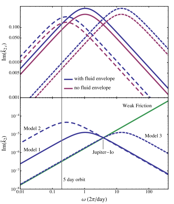
Figure 1: Theoretical curves for the tidal Love number of a Jupiter-mass planet as a function of the tidal forcing frequency, for several values of $R_{c}/R_{p}$ and $\eta$, each calibrated to satisfy the Jupiter-Io constraint. Top: The intrinsic Love number of the rocky core with (blue lines) and without (red lines) the presence of liquid envelope. Bottom: The effective Love number for the entire planet with fluid envelope. The density ratio of the core and envelope is $\rho_{c}/\rho_{F}=5$ and the core rigidity is $\mu=485\mathrm{~{}kbar}$ for all models. The other model parameters are as follows. Model 1 (blue solid line): $R_{c}/R_{p}=0.13$, $\eta=4.4\times 10^{9}$ $\mathrm{bar\,\cdotp s}$; Model 2 (blue long-dashed line): $R_{c}/R_{p}=0.19$, $\eta=2\times 10^{10}$ $\mathrm{bar\,\cdotp s}$; Model 3 (blue short-dashed line): $R_{c}/R_{p}=0.13$, $\eta=3.3\times 10^{8}$ $\mathrm{bar\,\cdotp s}$. Green solid line: weak friction theory with $\tau=0.06$ s (the lag time obtained using the value of $k_{2}/Q$ from Lainey et al. (2009) and assuming $k_{2}=0.38$).

Figure 1 presents three models for the tidal response $\mathrm{Im}(\tilde{k}_{2c})$ of Jupiter’s rocky core (upper panel), and the corresponding effective tidal response of the entire planet $\mathrm{Im}(\tilde{k}_{2})$ (lower panel). For each curve, different values of $\eta$ and $R_{c}$ were chosen such that the Jupiter-Io tidal dissipation constraint is satisfied (see also Fig. 10 of Remus et al. 2012a). Also plotted is the weak friction theory, similarly calibrated. For all the theoretical curves of Figure 1, we choose to fix $\mu$ and $\rho_{c}$, due to their smaller dynamical ranges. We note that of the remaining parameters, changing $\eta$ acts primarily to alter the transition frequency $\omega_{M}\sim{\mu\eta^{-1}}$, effectively moving the curve horizontally left-right, while changing $R_{c}$ effectively moves the curve up-down due to the strong dependence of $\tilde{k}_{2}$ on $R_{c}/R_{p}$.

From Figure 1, it is evident that the use of weak friction theory, which due to having only one parameter needs only one data point to be completely constrained, can lead to strong over- or under- estimation of tidal dissipation at different frequencies, as compared to more realistic models.

4 High-eccentricity migration of a giant planet with a rocky core

4.1 Orbital Evolution

We now compute the rates of high-e migration for a giant planet with a rocky core for different viscoelastic dissipation models depicted in Fig. 1, and compare the results with weak friction theory. We numerically carry out the sums in Eqs. (16)-(17) for different values of orbital eccentricity and a fixed final semi-major axis, i.e., the semi-major axis $a$ and eccentricity $e$ always satisfy $a(1-e^{2})\equiv a_{\mathrm{F}}=$constant, corresponding to a final circular orbital period of $5$ days.

Since the timescale for changing the planet’s spin is much shorter than the orbital evolution time, we assume that the planet is in the equilibrium spin state ($T_{z}=0$) at all times. For the weak friction theory, the result is [see Eq. (22)] $\Omega_{ps}/\Omega_{\rm peri}=(1+e)^{-3/2}f_{2}/f_{5}$, where $\Omega_{\rm peri}=\Omega/(1-e)^{3/2}$ is the orbital frequency at the pericenter. For general viscoelastic models, we set the right-hand-side of Eq. (16) to $0$ and numerically solve for the equilibrium spin rate $\Omega_{ps}$. The results are shown in Fig. 2. We note that while for the model parameters considered in Figs. 1-2, there exists a single $\Omega_{ps}$ for a given $e$ (for a given model), as in the weak friction theory, for other model parameters where the torque is created by a primarily elastic rather than viscous response ($\omega\mathrel{\hbox{\hbox to0.0pt{\hbox{\lower 3.0pt\hbox{$\sim$}}\hss}\hbox{\raise 2.0pt\hbox{$>$}}}}\omega_{M}$), it is possible to find multiple spin frequencies for which $T_{z}=0$, some of which are resonant in nature, for a given $e$. We discuss this interesting phenomenon in the Appendix.

Figure 2: Ratio of the pseudosynchronized spin frequency $\Omega_{\rm ps}$ to the pericenter frequency $\Omega_{\rm peri}$ for each of the viscoelastic models of Figure 1, as well as for the (analytical) weak friction model. Each blue curve corresponds to one of the Maxwell model curves depicted in Fig. 1. The green curve shows the result of the weak friction theory.

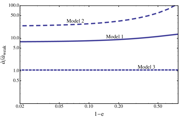
Figure 3: Ratio of the orbital decay rate $\dot{a}$ for different viscoelastic tidal dissipation models and $\dot{a}_{\rm weak}$ for the weak friction theory, as a function of eccentricity, for a fixed $a_{\mathrm{F}}=a(1-e^{2})$ corresponding to final mean motion period of $5$ days. Each curve corresponds to one of the blue Maxwell model curves of Fig. 1. In all cases, the weak friction theory is that of the green curve in Fig. 1.

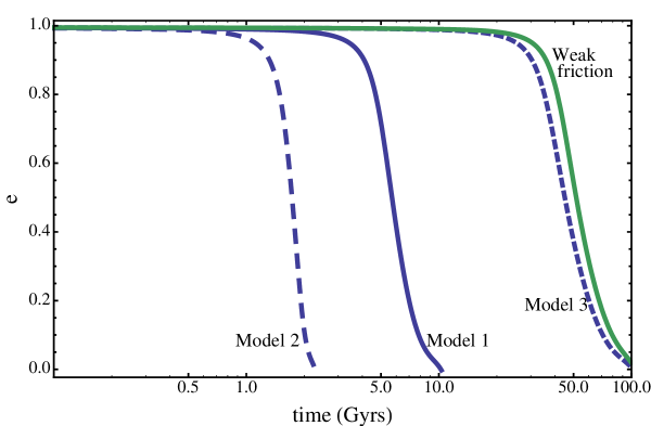
Figure 4: Eccentricity as a function of time, for an initial eccentricity of $0.9945$ and a final mean motion period of $5$ days. Each blue curve corresponds to one of the blue theoretical Maxwell model curves of Figure 1. The green curve corresponds to the weak friction theory of Fig. 1.

Figures 3 and 4 present the results of the orbital evolution for different viscoelastic tidal dissipation models. While all these models satisfy the same Jupiter-Io tidal $Q$ constraint as the weak friction theory, the predicted high-e migration rate can be easily larger, by a factor of 10 or more, than that predicted by the weak friction theory. For example, while it takes $\sim 100$ Gyrs to complete the orbital circularization in the weak friction theory, only $~{}10$ Gyrs is needed in Model 1 and only $\sim 2$ Gyrs is needed in Model 2.

4.2 Tidal heating of giant planets during migration

Many hot Jupiters are found to have much larger radii than predictions based on “standard” gas giant theory (e.g., Baraffe, Chabrier & Barman 2010). A number of possible explanations for the “radius inflation” have been suggested, including tidal heating (e.g., Bodenheimer, Lin & Mardling 2001, Bodenheimer, Laughlin & Lin 2003; Miller, Fortney & Jackson 2009; Ibgui et al. 2010; Leconte et al. 2010), the effect of thermal tides (Arras & Socrates 2010; Socrates 2013), enhanced envelope opacity (Burrows et al. 2007), double-diffusive envelope convection (Chabrier & Baraffe 2007; Leconte & Chabrier 2012) and Ohmic dissipation of planetary magnetic fields (Batygin & Stevenson 2010; Batygin, Stevenson & Bodenheimer 2011; but see Perna, Menou & Rauscher 2010; Huang & Cumming 2012; Menou 2012; Wu & Lithwick 2013; Rauscher & Menou 2013). It is possible that more than one mechanism is needed to explain all of the observed radius anomalies of hot Jupiters (see Fortney & Nettelmann 2010; Spiegel & Burrows 2013).

Several papers have already pointed out the potential importance of tidal heating in solving the radius anomaly puzzle (see above for references). In particular, Leconte et al. (2010) studied the combined evolutions of the planet’s orbit (starting from high eccentricity) and thermal structure including tidal heating, and showed that tidal dissipation in the planet provides a substantial contribution to the planet’s heat budget and can explain some of the moderately bloated hot Jupiters but not the most inflated objects (see also Miller et al. 2009; Ibgui et al. 2010). However, all these studies were based on equilibrium tide theory with a parametrized tidal quality factor $Q$ or lag time, and assume that the heating is distributed uniformly across the planet.

Here we study the heating of proto-hot-Jupiters via tidal dissipation in the core. To model this effect, we use the MESA code (Paxton et al. 2011, 2013) to evolve the internal structure of giant planets in conjunction with the orbital evolution starting from high eccentricity. We create a zero-age Jupiter-mass giant planet (initially hot and inflated) with an inert rocky core, for which we can prescribe a time-varying luminosity. Assuming the core is in thermal equilibrium with its surroundings, we consider the core luminosity to be equal to $\dot{E}$ as given by Eq. (17) (with $\Omega_{s}=\Omega_{\rm ps}$ such that $T_{z}=0$). We assume the planet starts at a high eccentricity of $e=0.9945$ and circularizes to a 5-day orbit, while conserving orbital angular momentum (so that $a_{F}=a(1-e^{2})$ at all times). These assumptions enable us to calculate $\dot{E}(t)$ and observe its effect on the radius of the planet.

Figure 5 presents the planet heating rate and radius vs age curves. Evidently, it is possible to inflate a proto-hot-Jupiter by up to $40\%$ via tidal heating in the core. However, this happens early in the planet’s evolution, around eccentricities of $0.6$, when the heating rate is largest. By the time the planet’s orbit has circularized ($e\mathrel{\raise 1.29167pt\hbox{$<$}\mkern-14.0mu\lower 2.58334pt\hbox{$\sim$}}0.05$), its radius is only $\sim 10\%$ larger than the zero-temperature planet and continues to decline over time. Therefore, regardless of the details of the tidal models, it appears that tidal heating cannot fully explain the population of observed hot Jupiters with significant radius inflation. Nevertheless, tidal effects can significantly delay the radius contraction of gas giants. By keeping the planet somewhat inflated until (possibly) another effect due to proximity to the host star takes over, tidal dissipation may still play an important role in the creation of inflated hot Jupiters.

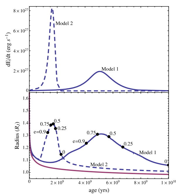
Figure 5: Top: Core luminosity due to viscoelastic tidal dissipation in a Jupiter-mass gas giant. The blue solid curve corresponds to Model 1 of Fig. 1, and the blue long-dashed curve corresponds to Model 2 of Fig. 1. Bottom: Evolution of radius vs time for each of the models (top), assuming an initial eccentricity of $0.9945$ and a final circularized orbital period of 5 days. The red solid curve has no tidal heating and asymptotes to the zero-temperature radius at later times. Black dots and labels on each curve denote when the particular planet model passes through that value of eccentricity in its orbital evolution. Note that since Model 2 is more dissipative than Model 1, the maximum heating rate and radius inflation (around $e=0.6$) occur earlier in time than Model 1.

Interestingly, these cooling curves suggest that if tidal dissipation in the core is indeed strong enough to play a significant role in circularizing the planet’s orbit, as we have shown to be possible in this paper, we may expect to observe a population of gas giants (proto-hot-Jupiters) in wide, eccentric orbits, which are nevertheless inflated more than expected (see Socrates et al. 2012a; Dawson & Murray-Clay 2013).

5 Conclusion

The physical mechanisms for tidal dissipations in giant planets are uncertain. Recent works have focused on mechanisms of dissipation in the planet’s fluid envelope, but it is not clear whether they are adequate to satisfy the constraints from the Solar system gas giants and the formation of close-in exoplanetary systems via high-$e$ migration.

In this paper, we have studied the possibility of tidal dissipation in the solid cores of giant planets. We have presented a general framework by which the effects of tidal dissipation on the spin and orbital evolution of planetary systems can be computed. This requires only one input - the imaginary part of the complex tidal Love number, ${\rm Im}[\tilde{k}_{2}(\omega)]$, as a function of the forcing frequency $\omega$. We discussed the simplest model of tidal response in solids - the Maxwell viscoelastic model, which is characterized by a transition frequency $\omega_{M}$, above which the solid responds elastically, below - viscously. Using the Maxwell model for the rocky/icy core, and including the effect of a non-dissipative fluid envelope, we have demonstrated that with a modest-sized rocky core and reasonable (but uncertain) physical core parameters, tidal dissipation in the core can account for the Jupiter-Io tidal-$Q$ constraint (Remus et al. 2012) and at the same time allows exoplanetary hot Jupiters to form via tidal circularization in the high-$e$ migration scenario. By contrast, in the often-used weak friction theory of equilibrium tide, when the tidal lag is calibrated with the Jupiter-Io constraint, hot Jupiters would not be able to go through high-$e$ migration within the lifetime of their host stars.

We have also examined the consequence of tidal heating in the rocky cores of giant planets. Such heating can lead to modest radius inflation of the planets, particularly when the planets are in the high-eccentricity phase ($e\sim 0.6$) during their high-$e$ migration.

As an interesting by-product of our study, we have shown that when ${\rm Im}(\tilde{k}_{2})$ exhibits nontrivial dependence on $\omega$ (as opposed to the linear dependence in the weak friction theory), there may exist multiple spin frequencies at which the torque on the planet vanishes (see Appendix A).

We emphasize that there remain large uncertainties in the physical properties of solid cores inside giant planets, including the size, density, composition, viscosity and elastic shear modulus. These uncertainties make it difficult to draw any definitive conclusion about the importance of core dissipation. Nevertheless, our study in this paper suggests that within the range of uncertainties, viscoelastic dissipation in the core is a possible mechanism of tidal dissipation in giant planets and has several desirable features when confronting the current observational constraints. Thus, core dissipation should be kept in mind as observations in the coming years provide more data on tidal dissipations in giant planets.

Appendix A Spin Equilibrium/Pseudosynchronization in Viscoelastic Tidal Models

In the weak friction theory, the tidal Love number ${\rm Im}({\tilde{k}_{2}})$ is a linear function of the tidal frequency $\omega$, and thus spin equilibrium ($T_{z}=0$) occurs at a unique value of $\Omega_{s}$, termed the pseudosynchronous frequency, for a given orbital eccentricity $e$. When ${\rm Im}({\tilde{k}_{2}})$ depends on $\omega$ in a more general way, as in the case of viscoelastic tidal models of giant planets, it is possible that multiple solutions for the equilibrium spin frequency $\Omega_{\rm ps}$ exist at a given $e$.

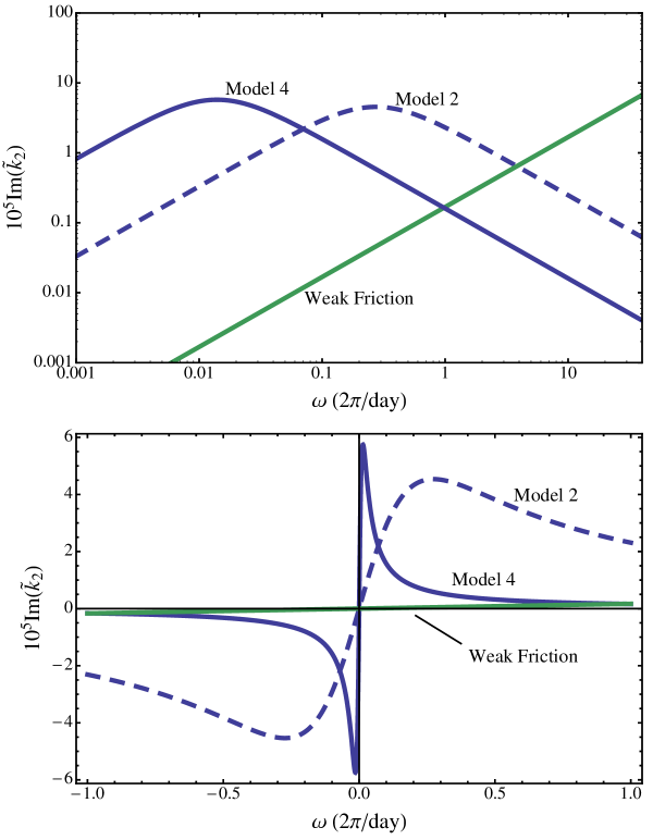
Figure 6: Theoretical curves for the tidal Love number of a Jupiter-mass planet as a function of the tidal forcing frequency. The blue dashed curve is the same as Model 2 of Fig. 1, and the green solid curve corresponds to the weak friction model of Fig. 1. The blue solid curve is a viscoelastic Maxwell model (model 4), with $R_{c}/R_{p}=0.2$ and $\eta=4\times 10^{11}$ $\mathrm{bar\,\cdotp s}$. In the top panel, the models are plotted on a log-log scale, as in Fig. 1, while in the bottom panel we plot the models on a linear scale to clarify how the shape of the tidal response curve leads to resonant equilibrium spin states.

The reason for the existence of multiple pseudo-synchronized spins can be understood in simple algebraic terms. For clarity here we demonstrate how multiple roots arise naturally even at low eccentricities. Consider Eq. (16), which we rewrite here to make the dependence on spin frequency explicit:

$$T_{z}={5\over 4\pi}T_{0}\sum_{m,N}m\,\left[W_{2m}F_{mN}(e)\right]^{2}\mathrm{Im}[{\tilde{k}}_{2}(N\Omega-m\Omega_{s})].$$ (38)

For very low eccentricities $e\ll 1$, the Hansen coefficients $F_{mN}$ are negligible for all except the following combinations of $(m,N)$: $(0,0)$, $(0,\pm 1)$,$(\pm 2,\pm 2)$, and $(\pm 2,\pm 3)$. We can then rewrite $T_{z}$ as

$$T_{z}=\mathrm{Im}[A\tilde{k}_{2}(2\Omega-2\Omega_{s})+B\tilde{k}_{2}(3\Omega-2\Omega_{s})],$$ (39)

with $A$ and $B$ real constants. Plugging in for $\tilde{k}_{2}$ using the Maxwell model (Eq. 32) (neglecting fluid envelope for simplicity), we have:

$$T_{z}=\bar{A}{(2\Omega-2\Omega_{s})\over 1+C(2\Omega-2\Omega_{s})^{2}}+\bar{B}{(3\Omega-2\Omega_{s})\over 1+C(3\Omega-2\Omega_{s})^{2}},$$ (40)

where $\bar{A}$, $\bar{B}$, and $C$ are constants. Thus, when solving for $\Omega_{s}$ from $T_{z}(\Omega_{s})=0$, it is obvious that upon finding the least common denominator, we end up solving a cubic equation for $\Omega_{s}$. The above discussion can be generalized to higher eccentricities: the pseudosynchronized spin $\Omega_{\rm ps}$ is determined by solving equations of increasingly higher (always odd) degree in $\Omega_{s}$.

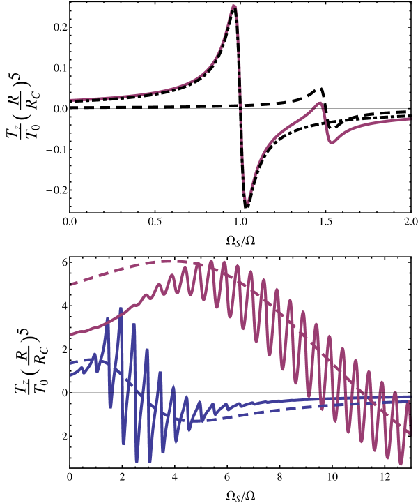
Figure 7: Tidal torque on the planet as a function of the spin frequency for different values of eccentricity and different tidal dissipation models. Top: Model 4 (solid blue) of Figure A1, for $e=0.13$. The black dot-dashed and dashed curves show the $(m,N)=(\pm 2,\pm 2)$ and $(\pm 2,\pm 3)$ terms of Eq. 40, respectively. The red curve shows their sum. The resonant features in each of the harmonics combine into three different zero-crossings in the sum. Bottom: Model 4 (solid) and Model 2 (dashed) of Figure A1. The red curves have $e=0.8$, while the blue curves have $e=0.5$. In order to fit all the curves on the same plot, we show $10T_{z}$ for the blue solid curve, and $0.1T_{z}$ for the red dashed curve. Equilibrium spins are determined by $T_{z}=0$. Evidently, in the case of Model 2, the viscoelastic response is not localized enough to permit more than one resonant solution.

The top panel of Figure A2 shows the two terms on the RHS of Eq. (40), as well as their sum, for the viscoelastic Model 4 of Figure A1 at an eccentricity of $0.13$. This demonstrates the way in which multiple solutions for $\Omega_{\mathrm{ps}}$ arise. Furthermore, we see that two (out of three) of the solutions are resonant in nature: that is, they occur, roughly, at multiples of $\Omega/2$, where $\Omega$ is the orbital frequency. This can be understood by considering that the viscoelastic response (Figure A1) is quite sharply peaked and localized. Each term on the RHS of Eq. (40) vanishes when $\Omega_{\rm s}=\Omega$ and $1.5\Omega$, respectively. Due to the sharply peaked nature of the viscoelastic response, to which $T_{z}$ is proportional, the sum of the two terms then shows resonant crossings at both of these values.

This generalizes easily to the case of arbitrary eccentricity, where each $(m,N)$ harmonic of the sum for $T_{z}$ (Eq. A1) vanishes when $N\Omega-m\Omega_{\rm s}=0$. The number and location of the resonant crossings then depends on the relative importance of each of the harmonics; the strongest crossing is expected to occur $\Omega_{\rm s}\sim\Omega_{\rm peri}$. This is demonstrated in Figure A2 (bottom) and Figure A3.

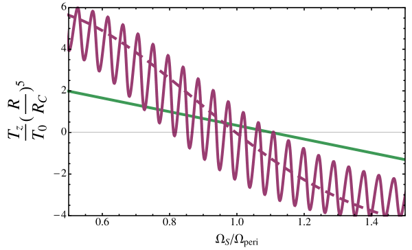
Figure 8: Tidal torque on the planet as a function of the ratio of spin frequency to pericenter frequency for $e=0.8$ and different tidal dissipation models. Red solid: Model 4 of Figure A1; red dashed: $0.1T_{z}$ for Model 2 of Figure A1; green solid: Weak friction model of Figure A1. Note that the equilibrium spin frequencies of the viscoelastic models can differ from the weak friction pseudosynchronous spin by as much as $\sim 10-20\%$.

Thus, the nonlinearity of the function ${\rm Im}[\tilde{k}_{2}(\omega)]$ of the viscoelastic Maxwell model is responsible for the existence of multiple pseudosynchronized spins. As shown in Figure A2 (bottom panel), there will not be multiple solutions if the viscoelastic response is not localized enough, compared with the mean motion frequency $\Omega$ (that is, the width of the resonant transition $\Delta\sim\omega_{M}\mathrel{\hbox{\hbox to0.0pt{\hbox{\lower 3.0pt\hbox{$\sim$}}\hss}\hbox{\raise 2.0pt\hbox{$>$}}}}\Omega$), and all important harmonics of $T_{z}$ are solidly on the viscous (linear) side of the Maxwell curve. On the other hand, there may exist multiple solutions when $\Delta\sim\omega_{M}\ll\Omega$ and the relevant tidal forcing frequencies lie on the elastic side of the Maxwell curve.

Finally, we note that all the resonant zero crossings of $T_{z}$ are stable (negative slope), while the non-resonant crossings are necessarily unstable (positive slope). The innermost and outermost crossings are always resonant. This phenomenon is analogous to that discussed by Makarov & Efroimsky (2013), who used a different model for viscoelastic dissipation in solid bodies to analyze the pseudosynchronization of telluric planets. They demonstrated the presence of multiple equilibrium spin solutions, and showed that only the resonant solutions are stable equilibria, thus concluding that the telluric planets possess no true (non-resonant) pseudosynchronous state.

The implications of our finding may be of practical interest when it becomes possible to measure the spin of exoplanets on eccentric orbits. We may then look for evidence of the existence of multiple stable spin equilibria in rocky planets or gas giants with rocky cores.

References

- (1) Alexander M.E., 1973, Astrophys. Space Sci., 23, 459
- (2) Arras P., Socrates A., 2010, ApJ, 714, 1
- (3) Baraffe I., Chabrier G., Barman T., 2010, Rep. Prog. Phys., 73, 016901
- (4) Batygin K., Stevenson D. J., 2010, ApJ, 714, L238
- (5) Batygin K., Stevenson D.J., Bodenheimer P.H., 2011, ApJ, 738, 1
- (6) Biot M.A., 1954, J. Appl. Phys., 25, 1385
- (7) Bodenheimer P., Lin D. N. C., Mardling R. A., 2001, ApJ, 548, 466
- (8) Bodenheimer P., Laughlin G., Lin D. N. C., 2003, ApJ, 592, 555
- (9) Burrows A., Hubeny I., Budaj J., Hubbard W.B., 2007, ApJ, 661, 502
- (10) Chabrier G., Baraffe I., 2007, ApJ, 661, L81
- (11) Chatterjee S., Ford E. B., Matsumura S., Rasio F. A., 2008, ApJ, 686, 580
- (12) Darwin G.H., 1879, Phil. Trans. R. Soc., 170, 1
- (13) Dawson R.I., Murray-Clay R.A., 2013, ApJ, 767, L24
- (14) Dermott S.F., 1979, Icarus, 37, 310
- (15) Eggleton P.P., Kiseleva L.G., Hut P., 1998, ApJ, 499, 853
- (16) Efroimsky M., Makarov V.V., 2013, ApJ, 764, 26
- (17) Fabrycky D., Tremaine S., 2007, ApJ, 699, 1298
- (18) Fortney J.J., Nettelmann N., 2010, Space Sci. Rev., 152, 423
- (19) Gavrilov S.V., Zharkov V.N., 1977, Icarus, 32, 443
- (20) Goldreich P., Nicholson P.D., 1977, Icarus, 30, 301
- (21) Goldreich P., Soter S., 1966, Icarus, 5, 375
- (22) Goldsby D. L., Kohlstedt D. L., 2001, J. Geophys. Res.,106, 11017
- (23) Goodman J., Lackner C., 2009, ApJ, 696, 2054
- (24) Guillot T., 2005, Ann. Rev. Earth Planet. Sci., 33, 493
- (25) Hansen B., 2012, ApJ, 757, 6
- (26) Henning W.G., O’Connell R.J., Sasselov D.D., 2009, ApJ, 707, 1000
- (27) Huang X., Cumming A., 2012, ApJ, 757, 47
- (28) Hut P., 1981, A&A, 99, 126
- (29) Ibgui L., Burrows A., Spiegel D.S., 2010, ApJ, 713, 751
- (30) Ioannou P.J., Lindzen R.S., 1993a, ApJ, 406, 252
- (31) Ioannou P.J., Lindzen R.S.,1993b, ApJ, 406, 266
- (32) Ivanov P.B., Papaloizou J.C.B., 2007, MNRAS, 376, 682
- (33) Jeanloz R., 1990, Annu. Rev. Earth Planet. Sci. 18, 357
- (34) Juric M., Tremaine S., 2008, ApJ, 686, 603
- (35) Katz B., Dong S., Malhotra R., 2011, Phys. Rev. Lett., 107, 181101
- (36) Lai D., 2012, MNRAS, 423, 486
- (37) Lainey V., Arlot J.-E., Karatekin Ö., van Hoolst T., 2009, Nature, 459, 957
- (38) Lainey V. et al., 2012, ApJ, 752, 14
- (39) Leconte J., Chabrier G., Baraffe I., Levrard B., 2010, A&A, 516, A64
- (40) Leconte J., Chabrier G., 2012, A&A, 540, A20
- (41) Love A., 1927, A Treatise on the Mathematical Theory of Elasticity (Dover, NY), p. 259
- (42) Lubow S.H., Tout C.A., Livio M., 1997, ApJ, 484, 866
- (43) Makarov V.V., Efroimsky M., 2013, ApJ, 764, 27
- (44) Mathis S., Le Poncin-Lafitte C., 2009, A&A, 497, 889
- (45) Matsumura S., Peale S. J., Rasio F. A., 2010, ApJ, 725, 1995
- (46) Menou K., 2012, ApJ, 745, 138
- (47) Militzer B., Hubbard W. B., Vorberger J., Tamblyn I., Bonev S. A., 2008, ApJ, 688, L45
- (48) Miller N., Fortney J.J., Jackson B., 2009, ApJ, 702, 1413
- (49) Mirouh G.M., Garaud P., Stellmach S., Traxler A. L., Wood T. S., 2012, ApJ, 750, 61
- (50) Mitrovica J.X., Forte, A.M., 2004, Earth Planet. Sci. Lett., 225, 177
- (51) Montagner J.P., Kennett, B.L.N., 1996, Geophys. J. Int. 125, 229
- (52) Murray C.D., Dermott, S.F., 2000, Solar System Dynamics. Cambridge Univ. Press, Cambridge.
- (53) Nagasawa M., Ida S., Bessho,T., 2008, ApJ, 678, 498
- (54) Naoz S., Farr W. M., Lithwick Y., Rasio F. A., Teyssandier J., 2011, Nature, 473, 187
- (55) Naoz S., Farr W.M., Rasio F.A., 2012, ApJ, 754, 36
- (56) Naoz S., Farr W. M., Lithwick Y., Rasio F. A., Teyssandier J., 2013, MNRAS, 431, 2155
- (57) Ogilvie G.I., 2009, MNRAS, 396, 794
- (58) Ogilvie G.I., 2013, MNRAS, 429, 613
- (59) Ogilvie G.I., Lin D.N.C., 2004, ApJ, 610, 477
- (60) Papaloizou J.C.B., Ivanov P.B., 2010, MNRAS, 407, 1631
- (61) Paxton B., et al., 2011, ApJS, 192, 3
- (62) Paxton B., et al., 2013, ApJS, 208, 4
- (63) Peale S.J., 1999, ARAA, 37, 533
- (64) Perna R., Menou K., Rauscher E., 2010, ApJ, 724, 313
- (65) Poirier J. P., Sotin C., Peyronneau J., 1981, Nature, 292, 225
- (66) Rasio F.A., Ford E.B., 1996, Science, 274, 954
- (67) Rauscher E., Menou K., 2013, ApJ, 764, 103
- (68) Remus F., Mathis S., Zahn J.-P., Lainey V., 2012a, A&A, 541, 165
- (69) Remus F., Mathis S., Zahn J.-P., 2012b, A&A, 544, 132
- (70) Sinclair A.T., 1983, in Dynamical Trapping and Evolution in the Solar System, ed. V.V. Markellos & Y. Kozai (D Reidel), p. 19
- (71) Socrates A., 2013, arXiv:1304.4121
- (72) Socrates A., Katz B., Dong S., Tremaine S., 2012a, ApJ, 750, 106
- (73) Socrates A., Katz B., Dong S., 2012b, preprint (arXiv:1209.5724)
- (74) Spiegel D.S., Burrows A., 2013, ApJ, 772, 76
- (75) Turcotte D.L., Schubert G., 2002, Geodynamics. Cambridge Univ. Press, Cambridge
- (76) Weidenschilling S.J., Marzari F., 1996, Nature, 384, 619
- (77) Wu Y., 2005, ApJ, 635, 688
- (78) Wu Y., Lithwick Y., 2011, ApJ, 735, 109
- (79) Wu Y., Lithwick Y., 2013, ApJ, 763, 13
- (80) Wu Y., Murray N.W., 2003, ApJ, 589, 605
- (81) Wu Y., Murray N.W., Ramshhai J.M., 2007, ApJ, 670, 820
- (82) Yoder C.F., Peale S.J., 1981, Icarus, 47, 1
- (83) Zhou J.-L., Lin D.N.C., Sun Y.-S., 2007, ApJ, 666, 423