Invariants of the single impurity Anderson model and implications for conductance functionals

Abstract

An exact relation between the conductance maximum $G_{0}$ at zero temperature and a ratio of lead densities is derived within the framework of the single impurity Anderson model: $G_{0}={\mathfrak{R}}[n]\frac{2e^{2}}{h}$, where ${\mathfrak{R}}[n]=4\Delta N_{{\cal L},x}\Delta N_{{\cal R},x}/(\Delta N_{{\cal L},x}+\Delta N_{{\cal R},x})^{2}$ and $\Delta N_{{\cal L},x}$, $\Delta N_{{\cal R},x}$ denote the excess density in the left/right lead at distance $x$ due to the presence of the impurity at the origin, $x=0$. The relation constitutes a parameter-free expression of the conductance of the model in terms of the ground state density that generalizes an earlier result to the generic case of asymmetric lead couplings. It turns out that the specific density ratio, ${\mathfrak{R}}[n]$, is independent of the distance to the impurity $x$, the (magnetic) band-structure and filling fraction of the contacting wires, the strength of the onsite interaction, the gate voltage and the temperature. Disorder induced backscattering in the contacting wires has an impact on ${\mathfrak{R}}$ that we discuss. Our result suggests that it should be possible, in principle, to determine experimentally the peak conductance of the Anderson impurity by performing a combination of measurements of ground-state densities.

1 Introduction

The single impurity Anderson model (SIAM) is one of the most important model system to understand correlation effects on electron transport through narrow constrictions and quantum dots. [1] The reason is that it is a minimal model featuring the two most important interaction induced phenomena in these systems, the Coulomb blockade and the Kondo effect. [2] Both these effects manifest themselves in the local spectral function, $A_{\text{d}}(E)$, of the impurity (single level quantum dot) as a triple peak structure, Hubbard side-bands and Abrikosov-Suhl resonance in the centre. For this reason, the spectral function and derived properties were in the focus of research for the last 40 years. [3] The charge susceptibility of the impurity has been obtained analytically already in the 1980ies with Bethe-Ansatz methods. [4, 5] It is not surprising that it received comparatively less attention than for instance the spin-susceptibility, simply because at the heart of the Kondo-effect is the screening of the impurity spin by conduction-band electrons. The manifestation of the associated correlation effects in the ground state density, $n(x)$, is more subtle. Such correlations are experimentally less accessible, namely only as a as shift of the impurity induced Friedel oscillations. [6]

The situation has changed recently, and the ground state density moved more into the active research focus. The reason is that the SIAM has become an important model system to investigate fundamental properties of the density functional theory (DFT). [7, 8, 9, 10, 11, 12, 13] From the point of view of DFT, the SIAM is an ideal test-bed, because of its analytical solvability and also because it allows for numerically highly accurate treatments based, e.g., on the numerical renormalization groug (NRG)[3] or the density matrix renormalization group (DMRG)[14, raas05, 16]. In particular, the earlier Bethe-Ansatz results[4] could be used in order to invert the relation between the impurity occupation $n(0)=N_{\text{d}}$ (summed over both spin directions) and its on site energy $\epsilon_{\text{d}}$ (“gate potential”) so as to obtain the exact exchange-correlation potential of this model analytically. [10, 11]

One important feature of the SIAM is that at zero temperature the Friedel sum rule holds true, which constitutes an exact relation between the ground-state density and the scattering phase of particles at the Fermi-energy[1]: $\delta_{\text{F}}=\pi N_{\text{d}}/2$. The relation is very convenient, because most theoretical treatments focus on the spectral-function, which is closely related to $N_{\text{d}}$, while experiments study the conductance, which is given via the identity (in units $2e^{2}/h$)

$$G = \mathcal{T}_{\text{0}}\sin(\delta_{\text{F}})^{2}$$ (1)

$$\mathcal{T}_{\text{0}} \equiv \frac{4|t_{\cal L}|^{2}|t_{\cal R}|^{2}}{(|t_{\cal L}|^{2}+|t_{\cal R}|^{2})^{2}}.$$ (2)

Friedel’s sum rule establishes the connection between the two. Here, $t_{\cal L,R}$ denote the hopping matrix elements, that connect the single site impurity with the left and right leads.

In the case of symmetric coupling, $t_{\cal L}{=}t_{\cal R}{\equiv}t^{\prime}$, $\mathcal{T}_{\text{0}}=1$ and Eq. (1) has a remarkable property: it establishes a relation between conductance and density that is free of microscopic model parameters, e.g., the onsite interaction $U$ and $t^{\prime}$. Based on this observation an important conclusion was drawn[9, 10, 12]: For symmetric coupling, any Schrödinger-type effective single particle theory, that produces the correct ground state density also reproduces the conductance. The Kohn-Sham (KS) formulation of DFT is such an effective single particle theory and therefore the frequently employed DFT-based transport scheme based on Landauer theory with KS-scattering states [17, 18, 19], is justified – as long as the symmetric SIAM applies and exact ground state functionals can be used.

In this work we provide an explicit formula for the conductance, $G$, that expresses the prefactor $\mathcal{T}_{\text{0}}$, Eq. (2), in a parameter free way as a ground state density ratio in the general case of asymmetric coupling, $t_{\cal L}\neq t_{\cal R}$. Specifically, we show that $\mathcal{T}_{\text{0}}$ is given by

$$\mathcal{T}_{\text{0}} = \mathfrak{R}[n]$$ (4)

$${\mathfrak{R}}[n] = \frac{4\Delta N_{{\cal L},x}\Delta N_{{\cal R},x}}{(\Delta N_{{\cal L},x}+\Delta N_{{\cal R},x})^{2}}$$ (5)

with $\Delta N_{{\cal L},x},\Delta N_{{\cal R},x}$ denoting the excess density in the left/right lead at distance $x$ due to the presence of the impurity in the origin, $x=0$.

Before we formally derive our result, we discuss several consequences. 1. Eq. (4) implies that $\mathfrak{R}$ is an invariant in the sense that it does not depend on the distance of the measurement point $x$ to the impurity site. 2. The invariance statement is very general. It is valid for any wire length (finite size or infinite) for any wire material (band-structure of a single channel wire and band filling) and for arbitrary Hubbard interaction $U$. Moreover, it also holds in equilibrium at non-zero temperature. The only condition is that the SIAM applies. 3. Eq. (4) provides a pure density-functional (units $2e^{2}/h$)

$${\cal G}[n]=\mathfrak{R}[n]\ \sin(\frac{\pi}{2}N_{\text{d}})^{2}$$ (6)

that constitutes an explicit parameter-free expression of the zero-temperature conductance in terms of the ground state density. The relation implies, in particular, the remarkable fact that the peak conductance can be determined numerically and at least in principle also experimentally, by a proper combination of ground state charge density measurements. Therefore, the ratio $\mathfrak{R}$ introduced here enjoys a fundamental status similar, in a sense, to the familiar scattering phase $\delta_{\text{F}}$. 4. Eq. (6) generalizes earlier statements for symmetric coupling – KS-based transport calculations employing the exact ground state XC-functional reproduce the exact many body conductance – to the experimentally very important case of asymmetric coupling.

2 Model definition and analytical derivations

The SIAM features a single level quantum dot

$$\hat{H}_{\text{QD}}{=}\epsilon_{\text{d}}{\hat{N}}_{\text{d}}+U\left(\hat{n}_{\mathrm{d}\uparrow}-\frac{1}{2}\right)\left(\hat{n}_{\mathrm{d}\downarrow}-\frac{1}{2}\right),$$ (7)

where ${\hat{N}}_{\text{d}}=\hat{n}_{\mathrm{d},\uparrow}+\hat{n}_{\mathrm{d},\downarrow}$ with $\hat{n}_{\mathrm{d},\sigma}=\hat{d}_{\sigma}^{\dagger}\hat{d}_{\sigma}^{\phantom{g}}$ and spin $\sigma=\uparrow,\downarrow$. The full model Hamiltonian is given by

$$\hat{H} = \hat{H}_{\text{QD}}+\hat{H}_{\text{T}}+\sum_{\alpha=\mathcal{L,R}}\hat{H}_{\alpha}$$ (8)

where the coupling to leads with a length of $M$ sites is described via

$$\hat{H}_{\alpha} {=} {-}\sum_{x,x^{\prime}=1,\sigma}^{M-1}t_{x,x^{\prime}}\left(c^{\dagger}_{\alpha\sigma,x}c_{\alpha\sigma,x^{\prime}}^{\phantom{g}}{+}\text{h.c.}\right),$$ (9)

$$\hat{H}_{\text{T}} {=} -\sum_{\sigma,\alpha}t_{\alpha}\left(c_{\alpha\sigma,1}^{\dagger}d_{\sigma}^{\phantom{g}}+d_{\sigma}^{\dagger}c^{\phantom{g}}_{\alpha\sigma,1}\right)\mathrm{.}$$ (10)

The operators $c^{\phantom{g}}_{\alpha\sigma,x},c_{\alpha\sigma,x}^{\dagger}$ denote fermionic annihilation and creation operators at site $x$. The rotation that we will employ with respect to the lead degrees of freedom, $\alpha={\cal L,R}$, does not mix spins. We subject the lead Hamiltonian (notation suppresses spin-index)

$$\sum_{\alpha}H_{\alpha}=-\sum_{x,x^{\prime}=1}^{M-1}t_{x,x^{\prime}}\sum_{\alpha}\ c^{\dagger}_{\alpha,x}c_{\alpha,x^{\prime}}+\text{h.c.}$$ (11)

to the standard rotation

$$\left(\begin{array}[]{c}c_{+,x}\\ c_{-,x}\end{array}\right) = \frac{1}{\tilde{t}}\left(\begin{array}[]{cc}t_{\cal L}&t_{\cal R}\\ -t_{\cal R}&t_{\cal L}\end{array}\right)\left(\begin{array}[]{c}c_{{\cal L},x}\\ c_{{\cal R},x}\end{array}\right)$$ (18)

and analogously for $c^{\dagger}_{{\cal L},x},c^{\dagger}_{{\cal R},x}$. The specific form (18) has been chosen such that the symmetric,“$+$”-channel couples to the quantum dot, with an effective coupling $\tilde{t}=\sqrt{|t_{\cal L}|^{2}+|t_{\cal R}|^{2}}$, while the anti-symmetric,“$-$”channel fully decouples. This decoupling naturally extends to multi-orbital impurities under the restriction of proportional coupling. After decoupling the model reads

$$\hat{H} {=} \hat{H}_{\text{QD}}+\sum_{\sigma}\tilde{t}(c^{\dagger}_{+\sigma,1}d^{\phantom{g}}_{\sigma}{+}d^{\dagger}_{\sigma}c^{\phantom{g}}_{+\sigma,1})+\hat{H}_{+}{+}\hat{H}_{-}$$ (19)

$$\hat{H}_{\beta}\!\! {=} \!\!\!\!\sum_{x,x^{\prime}=1}^{M-1}\!\!t_{x,x^{\prime}}\sum_{\sigma}\left(c^{\dagger}_{\beta\sigma,x}c^{\phantom{g}}_{\beta\sigma,x^{\prime}}{+}\text{h.c.}\right),\beta=\pm.$$ (20)

3 Invariants

Since the “$-$” channel decouples, we have $[\hat{H},\hat{H}_{-}]{=}0$, so the many-body eigenfunctions of $\hat{H}$ factorize into a non-interacting piece belonging to $\hat{H}_{-}$ and an interacting rest. In addition, $[\hat{H},\hat{N}_{-\sigma}]{=}[\hat{H}_{-},\hat{N}_{-\sigma}]{=}0$ implying that the number of particles per spin in the “${-}$”channel, $N_{-,\sigma}$, are good quantum numbers that come in addition to the total particle number, $N$.

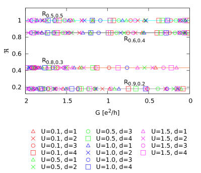
Figure 1: (Color on-line) Asymmetry factor $\mathfrak{R}$ vs. the conductance for a single impurity coupled to $M{=}16$ left and right lead sites via ($t_{\mathcal{L}}=0.5$, $t_{\mathcal{R}}=0.5$), ($t_{\mathcal{L}}=0.6$, $t_{\mathcal{R}}=0.4$), ($t_{\mathcal{L}}=0.8$, $t_{\mathcal{R}}=0.3$), and ($t_{\mathcal{L}}=0.9$, $t_{\mathcal{R}}=0.2$). $\mathfrak{R}$ was evaluated at distances $d=1,2,3,4$ from the impurity site and with local interactions $U=\pm 1.5,\pm 1,\pm 0.5,0.1$; the conductance was tuned by sweeping $\epsilon_{\text{d}}$ between $0$ to 2. Data is obtained by evaluating (5) (spin resolved) with DMRG ground-state densities at filling fraction corresponds to 32 fermions with total $S^{z}=0$. Data points for $\mathfrak{R}$ show no visible deviations from $\mathcal{T}_{\text{0}}$ (solid lines) fully confirming the prediction Eq. (4).

We now investigate consequences of the existance of the two invariants $N_{-\uparrow(\downarrow)}$. The thermodynamic excess densities at lead site $x$, that are induced by coupling to the impurity at $x=0$, can be written as

$$\Delta N_{\alpha,x}=\langle c^{\dagger}_{\alpha,x}c_{\alpha,x}\rangle-\langle c^{\dagger}_{-,x}c_{-,x}\rangle,\quad\alpha={\cal L,R}.$$ (21)

The density $\langle c^{\dagger}_{-,x}c_{-,x}\rangle$ of the antisymmetric channel is our reference density. Note, that it is equivalent to the particle density in the leads before wiring them to the impurity and therefore, can be determined directly in a suitable control measurement, at least in principle. The derivation of our result (4) proceeds by expressing the orginal lead densities in terms of their rotated counterparts. The rotation is norm conserving, hence $N_{{\cal L},x}{+}N_{{\cal R},x}=\langle c^{\dagger}_{+,x}c^{\phantom{g}}_{+,x}\rangle{+}\langle c^{\dagger}_{-,x}c^{\phantom{g}}_{-,x}\rangle$ so that trivially

$$\Delta N_{{\cal L},x}+\Delta N_{{\cal R},x}=\langle c^{\dagger}_{+,x}c^{\phantom{g}}_{+,x}\rangle-\langle c^{\dagger}_{-,x}c^{\phantom{g}}_{-,x}\rangle.$$ (22)

Similarly, we derive for the difference $N_{\cal L}-N_{\cal R}{=}\langle c^{\dagger}_{{\cal L},x}c^{\phantom{g}}_{{\cal L},x}\rangle-\langle c^{\dagger}_{{\cal R},x}c^{\phantom{g}}_{{\cal R},x}\rangle$:

$$\Delta N_{{\cal L},x}{-}\Delta N_{{\cal R},x} = {{\mathfrak{A}}}\left(\!\langle c^{\dagger}_{+,x}c^{\phantom{g}}_{+,x}\rangle{-}\langle c^{\dagger}_{-,x}c^{\phantom{g}}_{-,x}\rangle\!\right)$$ (23)

$${-} \mathcal{T}_{\text{0}}^{1/2}\left(\!\langle c^{\dagger}_{+,x}c^{\phantom{g}}_{-,x}\rangle{+}\langle c^{\dagger}_{-,x}c^{\phantom{g}}_{+,x}\rangle\!\right)$$

where we have introduced the relative asymmetry ${{\mathfrak{A}}}=(|t_{\cal L}|^{2}{-}|t_{\cal R}|^{2})/\tilde{t}^{2}$. Recalling Eq. (22) we obtain the identity

$$\frac{\Delta N_{{\cal L},x}{-}\Delta N_{{\cal R},x}}{\Delta N_{{\cal L},x}+\Delta N_{{\cal R},x}}{=}{{\mathfrak{A}}}-\mathcal{T}_{\text{0}}^{1/2}\frac{\langle c^{\dagger}_{+,x}c^{\phantom{g}}_{-,x}\rangle{+}\langle c^{\dagger}_{-,x}c^{\phantom{g}}_{+,x}\rangle}{\Delta N_{{\cal L},x}+\Delta N_{{\cal R},x}}$$ (24)

for any $x$ in the leads. The invariants $N_{-,\sigma}$ of the SIAM enter the final step of the proof. Since all eigenstates of $\hat{H}$ conserve the particle numbers in the “${-}$”channel, the second term on the rhs of Eq. (24) vanishes and we have

$$\frac{\Delta N_{{\cal L}\sigma,x}{-}\Delta N_{{\cal R}\sigma,x}}{\Delta N_{{\cal L}\sigma,x}+\Delta N_{{\cal R}\sigma,x}}={{{\mathfrak{A}}}}$$ (25)

with the spin-index restored. We arrive at the statement that the relative imbalance of the excess densities (total or per spin) equals everywhere the relative asymmetry of the junction irrespective of the onsite interaction $U$, or temperature. A spin-resolved version of our results, Eqs. (4,5), follows by squaring each side of Eq. (25) and then subtracting unity. Notice, that the derivation of Eq. (25) did not make specific reference to the band structure of the leads or the filling fraction. Hence, it holds for any lead band structure and in thermodynamic equilibrium at any temperature. Moreover, the derivation also does not make reference to the system size, $M$. Therefore, Eq. (25) is valid at any length of the left/right hand side wires.

3.1 Numerical check

In Fig. 1 we compare the asymmetry ratio $\mathfrak{R}$ with $\mathcal{T}_{\text{0}}$ for different conductance values (obtained by varying $\epsilon_{\text{d}}$ between zero and 2). We find $\mathfrak{R}$ (spin resolved), from the ground-state density that we obtain via a DMRG-calculation. The data, Fig. 1, exhibits no visible deviations from Eq. (4) within the broad set of parameter values that was tested. The residual deviations exhibit an even/odd effect with respect to the distance from the impurity; they are smaller than $10^{-5}$ (odd) and $10^{-8}$ (even) and can be attributed to numerical uncertainties in the DMRG-density.

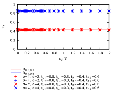
Figure 2: (Color on-line) Asymmetry factor $\mathfrak{R}_{\sigma}$ vs. the local potential $\epsilon_{\text{d}}$ for a single impurity coupled to ${M}{=}16$ left and right lead sites, via spin dependent hybridization $t_{\mathcal{L},\uparrow}=0.8$, $t_{\mathcal{L},\downarrow}=0.3$ and $t_{\mathcal{R},\uparrow}=0.4$, $t_{\mathcal{R},\downarrow}=0.6$ measured at distances $d=2,4$ from the impurity site and for local interactions of $U=0,0.01.0.1,0.3,0.5,0.7,1.0,1.52.0,3.0,5.0$ for each values of $\epsilon_{\text{d}}$, and 32 fermions with total $S^{z}=0$.

4 Extension to magnetic leads

In recent measurements of the magneto-resistance of individual molecules a spin-dependent coupling $t_{\alpha,\sigma}$ was introduced to explain the experiments and motivated via DFT-based transport studies. [21, 22]. In this spirit, we generalize our model now including the possibility of magnetic electrodes:

$$\hat{H}_{\alpha} {=} {-}\sum_{x,x^{\prime}=1,\sigma}^{M-1}t_{x,x^{\prime},\sigma}\left(\hat{c}_{\alpha\sigma,x}^{\dagger}\hat{c}_{\alpha\sigma,x^{\prime}}^{\phantom{g}}{+}\text{h.c.}\right)$$ (26)

$$\hat{H}_{\text{T}} {=} -\sum_{\alpha,\sigma}t_{\alpha\sigma}\left(\hat{c}_{\alpha\sigma,1}^{\dagger}\hat{d}_{\sigma}^{\phantom{g}}+\hat{d}_{\sigma}^{\dagger}\hat{c}_{\alpha\sigma,1}^{\phantom{g}}\right)\mathrm{.}$$ (27)

The rotation (18) operates on each spin sector separately, and each spin direction has its own invariant, $N_{-\sigma}$. Hence, we immediately conclude ${{\mathcal{T}_{\text{0}}}_{\sigma}}=\mathfrak{R}_{\sigma}[n_{\sigma}]$ ($n_{\sigma}$: particle number density per spin in the ground-state),

$${\mathfrak{R}}_{\sigma}[n_{\sigma}] = \frac{4\Delta N_{{\cal L}\sigma,x}\Delta N_{{\cal R}\sigma,-x}}{(\Delta N_{{\cal L}\sigma,x}+\Delta N_{{\cal R}\sigma,-x})^{2}}$$ (28)

$${\mathcal{T}_{\text{0}}}_{\sigma} \equiv \frac{4|t_{{\cal L}\sigma}|^{2}|t_{{\cal R}\sigma}|^{2}}{(|t_{{\cal L}\sigma}|^{2}+|t_{{\cal R}\sigma}|^{2})^{2}}.$$ (29)

Again, we subject our analytical findings to a numerical test. In Fig. 2 we display asymmetry ratios $\mathfrak{R}_{\sigma}$ for asymmetric, spin-dependent couplings to non-magnetic wires. The data fully confirms our analysis, Eqs. (28,29).

5 Discussion

The results presented so far crucially rely upon the existance of two extra invariants in the SIAM, $N_{-\uparrow(\downarrow)}$. They originate from two special features: (i) there is only a single level (more precisely: proportional coupling is required in the sense of Ref.[23]) (ii) all leads have an identical electronic structure. Since both of these features capture important aspects but not all of physical reality, one may ask about the effect of perturbations.

5.1 Competing orbitals

A general discussion of possible multi-orbital terms that could complement $\hat{H}_{\text{QD}}$ in realistic situations is extremely complicated and not indicated here. Instead, we can recall that the density modulation in the leads, $\Delta N_{\cal L,R}$, is due to the change in occupation of the frontier-levels of the QD and as such a Fermi-surface effect. Therefore, in the spirit of the Fermi-liquid theory any microscopic description is justified that correctly represents this low-energy sector. And because of this, the SIAM is indeed very successful when describing the ($S{=}1/2$) Kondo-effect as it is frequently observed in experiments[24]; this includes details like the temperature scaling.

5.2 Disorder in the leads

Here, we offer a first test of the assumption (ii) and ask about the effect of small differences in the band structures of the left/right wires. We subject the leads to onsite disorder, $\hat{H}_{\text{dis}}$, where the local energies are drawn from a box distribution of width $W$. The term in $\hat{H}$ that introduces the difference between left/right leads reads

$$\hat{H}_{\text{dis}}{=}\!\!\sum_{\sigma,x=1}^{M}v_{x}\left(c^{\dagger}_{{\cal L}\sigma,x}c^{\phantom{g}}_{{\cal L}\sigma,x}{-}c^{\dagger}_{{\cal R}\sigma,x}c^{\phantom{g}}_{{\cal R}\sigma,x}\right){=}\hat{H}_{\text{as}}{+}\hat{V}_{\text{T}}$$ (30)

where

$$\hat{H}_{\text{as}} = {{\mathfrak{A}}}\sum_{\sigma,x}v_{x}\left(c^{\dagger}_{+\sigma,x}c^{\phantom{g}}_{+\sigma,x}{-}c^{\dagger}_{-\sigma,x}c^{\phantom{g}}_{-\sigma,x}\right)$$

$$\hat{V}_{\text{T}} = -\mathcal{T}_{\text{0}}^{1/2}\sum_{\sigma,x}v_{x}\left(c^{\dagger}_{+\sigma,x}c^{\phantom{g}}_{-\sigma,x}+c^{\dagger}_{-\sigma,x}c^{\phantom{g}}_{+\sigma,x}\right).$$ (31)

The first term, $\hat{H}_{\text{as}}$, still respects the basic symmetries of the SIAM outlined below Eq. (20). Its most important effect is to modulate $\langle c^{\dagger}_{\beta\sigma,x}c^{\phantom{g}}_{\beta\sigma,x}\rangle$ in space with an amplitude that vanishes for symmetric coupling, when ${{\mathfrak{A}}}\to 0$.

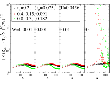
Figure 3: (Color on-line) Mean deviation of ${\mathfrak{R}}_{\text{dis},x}$ (see text) from $\mathcal{T}_{\text{0}}$ normalized by the disorder strength $W$ and the level broadening $\Gamma^{1/2}$. Data is given at even sites away from the impurity for increasing disorder $W=10^{-4},10^{-3},10^{-2},0.1$ and different couplings $t_{\cal L,R}$. ($\mathcal{T}_{\text{0}}=0.43235$ is fixed, $U=0$, $M{=}256$ and $\epsilon_{\text{d}}=0.1$.) It is seen here that even in the presence of moderate disorder ${\mathfrak{R}}_{\text{dis},x}$ can give an estimate for $\mathcal{T}_{\text{0}}$ with accuracy $\sim W\Gamma^{1/2}$ if one focusses on the near impurity region, where $x$ is much smaller than the mean free path, $\ell$. (We recall that in the present lead model $\ell\approx 100/W^{2}$.[25])

The disorder term $\hat{V}_{\text{T}}$ includes tunnelling between the “$+$” and “$-$” channels, so that $N_{-\uparrow(\downarrow)}$ are no longer conserved in its presence; the second term on the rhs of Eq. (24) no longer vanishes, in general.

To complement the qualitative discussion, we have performed a numerical simulation in order to quantify the effect of the symmetry-breaking terms. We define an observable ${\mathfrak{R}}_{\text{dis},x}$ which is similar to ${\mathfrak{R}}_{x}$ of Eq. (4), with the difference that we approximate $\langle c^{\dagger}_{-,x}c^{\phantom{g}}_{-,x}\rangle\approx(\bar{N}_{{\cal L},x}{+}\bar{N}_{{\cal R},x})/2$ where $\bar{N}_{{\cal L},x},\bar{N}_{{\cal R},x}$ denote the particle density in the the leads in the absense of a coupling to the impurity site. The object ${\mathfrak{R}}_{\text{dis},x}$ is interesting to study since it is an explicit density functional that reduces to the exact expression in the limit $W{\to}0$ and is directly accessible to experimental measurements, at least in principle. Importantly, our simulations, Fig. 3, suggests that in the case of asymmetric coupling, ${\mathfrak{R}}_{\text{dis}}$ exhibits fluctuations about $\mathcal{T}_{\text{0}}$ of a size $\sim cW\sqrt{\Gamma}/|t_{{\cal L},{\cal R}}|^{3/2}$ with a factor $c\approx 2$. This result is encouraging, because it shows that disorder effects can be well controlled by going to weakly coupled QDs. Hence, we believe that there are promising prospects that even in the presence of moderate disorder one can still estimate the maximum conductance with good accuracy in experiments by performing a sequence of ground-state density measurements.

- [1] \NameHewson A. C. \BookThe Kondo Problem to Heavy Fermions (Cambridge Studies in Magnetism, New York, N.Y.) 1995.
- [2] \NameKondo J. \REVIEWProgress of Theoretical Physics32196437.
- [3] \NameBulla R., Costi T. Pruschke T. \REVIEWRev. Mod. Phys.802008395.
- [4] \NameTsvelik A. Wiegmann P. \REVIEWAdv. in Phys.321983453.
- [5] \NameAndrei N., Furuya K. Lowenstein J. H. \REVIEWRev. Mod. Phys.551983331.
- [6] \NameAffleck I., Borda I. Saleur H. \REVIEWPhys. Rev. B772008180404(R).
- [7] \NameMera H. Niquet Y. \REVIEWPhys. Rev. Lett.1052010216408.
- [8] \NameEvers F. Schmitteckert P. \REVIEWPhys. Chem. Chem. Phys.13201114417.
- [9] \NameTröster P., Schmitteckert P. Evers F. \REVIEWPhys. Rev. B852012115409.
- [10] \NameBergfield J. P., Liu Z., Burke K. Stafford C. A. \REVIEWPhys. Rev. Lett.1082012066801.
- [11] \NameLiu Z., Bergfield J. P., Burke K. Stafford C. A. \REVIEWPhys. Rev. B852012155117.
- [12] \NameStefanucci G. Kurth S. \REVIEWPhys. Rev. Lett.1072011216401.
- [13] \NameKurth S. Stefanucci G. \REVIEWPhys. Rev. Lett.1112013 030601
- [14] \NameWhite S. R. \REVIEWPhys. Rev. Lett.6919922863.
- [15] \NameRaas G. Uhrig G.\REVIEWEuro. Phys. Journal B452005293.
- [16] \NamePeters R. \REVIEWPhys. Rev. B842011075139.
- [17] \NameArnold A., Weigend F. Evers F. \REVIEWJ. Chem. Phys.1262007174101.
- [18] \NameBrandbyge M., Mozos J.-L., Ordejon P., Taylor J. Stokbro K. \REVIEWPhys. Rev. B652002165401.
- [19] \NameCuevas J. C. Scheer E. \BookMolecular Electronics: An Introduction to Theory and Experiment World Scientific Series in Nanotechnology and Nanoscience (World Scientific) 2010.
- [20] \NameBohr D., Schmitteckert P. Wölfle P. \REVIEWEurophys. Lett.732006246.
- [21] \NameSchmaus S., Bagrets A., Nahas Y., Yamada T. K., Bork A., Bowen M., Beaurepaire E., Evers F. Wulfhekel W. \REVIEWNature Nanotechnology62011185.
- [22] \NameBagrets A., Schmaus S., Jaafar A., D. K., Kazu T., Alouani M., Wulfhekel W. Evers F. \REVIEWNano Lett.1220125131.
- [23] \NameMeir Y. Wingreen N. \REVIEWPhys. Rev. Lett.6819922512.
- [24] \NameScott G. Natelson D. \REVIEWACS Nano420103560.
- [25] \NameKramer B. MacKinnon A. \REVIEWRep. Prog. Phys.5619931469.