Power-law models for infectious disease spread

Abstract

Short-time human travel behaviour can be described by a power law with respect to distance. We incorporate this information in space–time models for infectious disease surveillance data to better capture the dynamics of disease spread. Two previously established model classes are extended, which both decompose disease risk additively into endemic and epidemic components: a spatio-temporal point process model for individual-level data and a multivariate time-series model for aggregated count data. In both frameworks, a power-law decay of spatial interaction is embedded into the epidemic component and estimated jointly with all other unknown parameters using (penalised) likelihood inference. Whereas the power law can be based on Euclidean distance in the point process model, a novel formulation is proposed for count data where the power law depends on the order of the neighbourhood of discrete spatial units. The performance of the new approach is investigated by a reanalysis of individual cases of invasive meningococcal disease in Germany (2002–2008) and count data on influenza in 140 administrative districts of Southern Germany (2001–2008). In both applications, the power law substantially improves model fit and predictions, and is reasonably close to alternative qualitative formulations, where distance and order of neighbourhood, respectively, are treated as a factor. Implementation in the R package surveillance allows the approach to be applied in other settings.

FLA

and T1Funded by the Swiss National Science Foundation (project #137919).

1 Introduction

The surveillance of infectious diseases constitutes a key issue of public health and modelling their spread is basic to the prevention and control of epidemics. An important task is the timely detection of disease outbreaks, for which popular methods are the Farrington algorithm [Farrington et al. (1996), Noufaily et al. (2013)] and cumulative sum (CUSUM) likelihood ratio detectors inspired by statistical process control [Höhle and Paul (2008), Höhle, Paul and Held (2009)]. As opposed to such prospective surveillance, retrospective surveillance is concerned with explaining the spread of an epidemic through statistical modelling, thereby assessing the role of environmental and socio-demographic factors or contact networks in shaping the evolution of an epidemic. The spatio-temporal data for such modelling primarily originate from routine public health surveillance of the occurrence of infectious diseases and is ideally accompanied by additional data on influential factors to be accounted for. Surveillance data are available in different spatio-temporal resolutions, each type requiring an appropriate model framework.

This paper covers both a spatio-temporal point process model for individual-level data [proposed by Meyer, Elias and Höhle (2012) and motivated by the work of Höhle (2009)] and a multivariate time-series model for aggregated count data [established by Held and Paul (2012) and earlier work]. Although these two models are designed for different types of spatio-temporal surveillance data, both are inspired by the approach of Held, Höhle and Hofmann (2005) decomposing disease risk additively into “endemic” and “epidemic” components. The endemic component captures exogenous factors such as population, socio-demographic variables, long-term trends, seasonality, climate, or concurrent incidence of related diseases (all varying in time and/or space). Explicit dependence between cases, that is, infectiousness, is then introduced through epidemic components driven by the observed past.

To describe disease spread in space, both models account for spatial interaction between units or individuals, respectively, but up to now, this has been incorporated rather crudely. The point process model used a Gaussian kernel to capture spatial interaction, and the multivariate time-series model restricted epidemic spread from time $t$ to $t+1$ to adjacent regions. However, a simple form of dispersal can be motivated by the findings of Brockmann, Hufnagel and Geisel (2006): they inferred from the dispersal of bank notes in the United States that (short-time) human travel behaviour can be well described by a decreasing power law of the distance $x$, that is, $f(x)\propto x^{-d}$ with positive decay parameter $d$. An important characteristic of this power law is its slow convergence to zero (“heavy tail”), which in our application enables occasional long-range transmissions of infectious agents in addition to principal short-range infections. In the words of Brockmann, Hufnagel and Geisel (2006), their results “can serve as a starting point for the development of a new class of models for the spread of human infectious diseases”. Power laws are well known from the work by Pareto (1896) for the distribution of income and Zipf (1949) for city sizes and word frequencies in texts. They describe the distribution of earthquake magnitudes [Gutenberg and Richter (1944)] and many other natural phenomena [see Newman (2005), Pinto, Mendes Lopes and Machado (2012), for a review of power laws]. Liljeros et al. (2001) reported on a power-law distribution of the number of sexual partners, and Albert and Barabási (2002) review recent advances in network theory including scale-free networks where the number of edges is distributed according to a power law. Interestingly, a power law was also used as the distance decay function in geographic profiling for serial violent crime investigation [Rossmo (2000)] as well as in an application of this technique to identify environmental sources of infection [Le Comber et al. (2011)]. Examples of power-law transmission kernels to model the spatial dynamics of infectious diseases can be found in plant epidemiology [Gibson (1997), Soubeyrand et al. (2008)] and in models for the 2001 UK foot-and-mouth disease epidemic [Chis Ster and Ferguson (2007)]. Recently, Geilhufe et al. (2014) found that using (fixed) power-law weights between regions performed better than real traffic data in predicting influenza counts in Northern Norway. In both models for spatio-temporal surveillance data presented in the following sections, the power law will be estimated jointly with all other unknown parameters. Since the choice of a power law is a strong (yet well motivated) assumption, a comparison with alternative qualitative formulations is provided.

This paper is organised as follows: in Sections 2 and 3, respectively, the two model frameworks are reviewed and extended with power-law formulations for the spatial interaction of units. In Section 4 surveillance data on invasive meningococcal disease (IMD) and influenza are reanalysed using power laws and alternative qualitative approaches to be evaluated against previously used models for these data. We close with some discussion in Section 5 and a software overview in the Appendix. The paper is accompanied by animations (Supplement A) and further supplementary material [Supplement B: Meyer and Held (2014)].

2 Individual-level model

2.1 Introduction

The spatio-temporal point process model proposed by Meyer, Elias and Höhle (2012) is designed for time–space-mark data $\{(t_{i},\mathbf{s}_{i},\mathbf{m}_{i})\dvtx i=1,\ldots,n\}$ of individual case reports to describe the occurrence of infections (‘events’) and their potential to trigger secondary cases. Formally, the model characterises a point process in a region $\mathbf{W}$ observed during a period $(0,T]$ through the conditional intensity function

$$\lambda(t,\mathbf{s})=\nu_{[t][\mathbf{s}]}\rho_{[t][\mathbf{s}]}+\sum_{j\dvtx t_{j}<t}\eta_{j}\cdot g(t-t_{j})\cdot f\bigl{(}\|\mathbf{s}-\mathbf{s}_{j}\|\bigr{)}.$$ (1)

Related models are the purely temporal, “self-exciting” process proposed by Hawkes (1971), the spatio-temporal epidemic-type aftershock-sequences (ETAS) model from earthquake research [Ogata (1998)], the point process models discussed by Diggle (2007), and an additive-multiplicative point process model for discrete-space surveillance data proposed by Höhle (2009).

The first endemic component in model (1) consists of a log-linear predictor $\log(\nu_{[t][\mathbf{s}]})=\beta_{0}+\bolds{\beta}^{\top}\mathbf{z}_{[t][\mathbf{s}]}$ proportional to an offset $\rho_{[t][\mathbf{s}]}$, typically the population density. Both the offset and the exogenous covariates are given piecewise constant on a spatio-temporal grid (e.g., week${}\times{}$district), hence the notation $[t][\mathbf{s}]$ for the period which contains $t$ in the region covering $\mathbf{s}$. In the IMD application in Section 4.1, $\mathbf{z}_{[t][\mathbf{s}]}=([t],\sin(\omega\cdot[t]),\cos(\omega\cdot[t]))^{\top}$ incorporates a time trend with one sinusoidal wave of frequency $\omega=2\pi/365$.

A purely endemic intensity model without the observation-driven epidemic component is equivalent to a Poisson regression model for the aggregated number of cases on the chosen spatio-temporal grid. However, with an epidemic component the intensity process depends on previously infected individuals and becomes “self-exciting.” Specifically, the epidemic force of infection at $(t,\mathbf{s})$ is the superposition of the infection pressures caused by each previously infected individual $j$. The individual infection pressure is weighted by the log-linear predictor $\log(\eta_{j})=\gamma_{0}+\bolds{\gamma}^{\top}\mathbf{m}_{j}$, which models effects of individual/infection-specific characteristics $\mathbf{m}_{j}$ such as the age of the infective. Regional-level covariates could also be included in $\mathbf{m}_{j}$, for example, to model ecological effects on infectivity. Note, however, since the epidemic is modelled through a point process, the susceptible “population” consists of the continuous observation region $\mathbf{W}\subset\mathbb{R}^{2}$ and is thus infinite. Consequently, the model cannot include information on susceptibles, nor an autoregressive term as in time-series models.

Decreasing infection pressure of individual $j$ over space and time is described by $f(x)$ and $g(t)$, parametric functions of the spatial distance $x$ and of the elapsed time $t$ since individual $j$ became infectious, respectively. The spatial interaction could also be described more generally by a nonisotropic function $f_{2}(\mathbf{s})$ of the vector $\mathbf{s}$ to the host, for example, to incorporate the dominant wind direction in vector-borne diseases. However, in our application, $f$ essentially reflects people’s movements and we assume that $f_{2}(\mathbf{s})=f(\|\mathbf{s}\|)$ only depends on the distance to the host. Note that we project geographic coordinates into a planar coordinate reference system to apply Euclidean geometry. Meyer, Elias and Höhle (2012) used an isotropic Gaussian kernel

$$f(x)=\exp\biggl{(}-\frac{x^{2}}{2\sigma^{2}}\biggr{)}$$ (2)

with scale parameter $\sigma$. In what follows, we propose an alternative spatial interaction function, which allows for occasional long-range transmission of infections: a power law.

2.2 Power-law extension

The basic power law $f(x)=x^{-d}$, $d>0$, is not a suitable choice for the distance decay of infectivity since it has a pole at $x=0$. For $x\geq\sigma>0$, $x^{-d}$ is the kernel of a Pareto density, but a shifted version to the domain $\mathbb{R}_{0}^{+}$, known as Pareto type II and sometimes named after Lomax (1954), has density kernel

$$f(x)=(x+\sigma)^{-d}\propto\biggl{(}1+\frac{x}{\sigma}\biggr{)}^{-d}$$ (3)

[see Figure 1(a)]. Note that there is no need for the spatial interaction function to be normalised to a density. It is actually more closely related to correlation functions known from stationary random field models for geostatistical data [Chilès and Delfiner (2012)]. For instance, the rescaled version $(1+x/\sigma)^{-d}$ is a member of the Cauchy class introduced by Gneiting and Schlather (2004), which provides asymptotic power-law correlation as $x\to\infty$.

(a) Power-law kernel	(b) Lagged power law	(c) Student kernel

Figure 1: Power-law kernels as a function of the distance $x$ for various choices of the decay parameter $d>0$ and $\sigma=5$.

For short-range travel within 10 km, Brockmann, Hufnagel and Geisel (2006) found a uniform distribution instead of power-law behaviour, which suggests an alternative formulation with a “lagged” power law:

$$f(x)=\cases{1,&\quad for $x\leq\sigma$,\vspace*{3pt}\cr\displaystyle\biggl{(}\frac{x}{\sigma}\biggr{)}^{-d},&\quad otherwise.}$$ (4)

Spatial interaction is now constant up to the change point $\sigma>0$, followed by a power-law decay for larger distances [see Figure 1(b)]. A similar kernel was used by Deardon et al. [(2010), therein called “geometric”] for the 2001 UK foot-and-mouth disease epidemic, additionally limiting spatial interaction to a prespecified upper-bound distance.

A change-point-free kernel also unifying intended short-range and long-range characteristics is the Student kernel

$$f(x)=\bigl{(}x^{2}+\sigma^{2}\bigr{)}^{-d}\propto\biggl{(}1+\biggl{(}\frac{x}{\sigma}\biggr{)}^{2}\biggr{)}^{-d}$$ (5)

with scale parameter $\sigma$ and shape (decay) parameter $d$ [see Figure 1(c)]. This kernel implements a power law of the squared distance and is known as the ‘Cauchy model’ in geostatistics [Chilès and Delfiner (2012)]. For $d>0.5$, it describes a Student distribution with $2d-1$ degrees of freedom.

To investigate the appropriateness of the assumed power-law decay, we also estimate an unconstrained step function

$$f(x)=\sum_{k=0}^{K}\alpha_{k}\mathbh{1}(x\in I_{k}),$$ (6)

which corresponds to treating the distance $x$—categorised into consecutive intervals $I_{k}$—as a qualitative variable.

2.3 Inference

Model parameters are estimated via maximization of the full (log-)likelihood, applying a quasi-Newton algorithm with analytical gradient and Hessian [see Meyer and Held (2014), Section 1.1]. We estimate kernel parameters on the log-scale to avoid constrained optimization. For the step function, $\alpha_{0}=1$ is fixed to ensure identifiability.

The point process likelihood incorporates the integral of $f_{2}(\mathbf{s})$ over shifted versions of the observation region $\mathbf{W}$, which is represented by polygons. Similar integrals arise for the partial derivatives of $f_{2}(\bm{s})$ in the score function and approximate Fisher information. Except for the step function kernel (6), this requires a method of numerical integration such as the two-dimensional midpoint rule with an adaptive bandwidth, which was found to be best suited for the Gaussian kernel [Meyer, Elias and Höhle (2012)]. For the other kernels we use a more sophisticated approach inspired by product Gauss cubature over polygons [Sommariva and Vianello (2007)]. This cubature rule is based on Green’s theorem, which relates the double integral over the polygon to a line integral along the polygon boundary. Its efficiency can be greatly improved in our specific case by taking analytical advantage of the isotropy of $f_{2}$, after which numerical integration remains in only one dimension [see Meyer and Held (2014), Section 2.4]. Regardless of any sophisticated cubature rule, the required integration of $f_{2}$ over $n$ polygons in the log-likelihood is the part that makes model fitting cumbersome: it introduces numerical errors which have to be controlled such that they do not corrupt numerical likelihood maximization, and it increases computational cost by several orders of magnitude. For instance, in our IMD application in Section 4.1 a single likelihood evaluation would only take 0.02 seconds if we used a constant spatial interaction function $f(x)\equiv 1$, where the integral does not depend on parameters being optimised and simply equals the area of the polygonal domain. For the Gaussian kernel, a single evaluation takes about 5 seconds, the step function takes 7 seconds, and the power law and Student kernel take about 20 seconds. The above and all following runtime statements refer to total CPU time at 2.80GHz (real elapsed time is shorter since some computations run in parallel on multiple CPUs).

3 Count data model

3.1 Introduction

The multivariate time-series model established by Held and Paul (2012) [see also Paul and Held (2011), Paul, Held and Toschke (2008), Held, Höhle and Hofmann (2005)] is designed for spatially and temporally aggregated surveillance data, that is, disease counts $Y_{it}$ in regions $i=1,\ldots,I$ and periods $t=1,\ldots,T$. Formally, the counts $Y_{it}$ are assumed to follow a negative binomial distribution

$$Y_{it}|\mathbf{Y}_{\cdot,t-1}\sim\operatorname{NegBin}(\mu_{it},\psi),\qquad i=1,\ldots,I,t=1,\ldots,T$$

with additively decomposed mean

$$\mu_{it}=\nu_{it}e_{it}+\lambda_{it}Y_{i,t-1}+\phi_{it}\sum_{j\neq i}w_{ji}Y_{j,t-1},$$ (7)

and overdispersion parameter $\psi$ such that the conditional variance of $Y_{it}$ is $\mu_{it}(1+\psi\mu_{it})$. The Poisson distribution results as a special case if $\psi=0$. In (7), the first term represents the endemic component similar to the point process model (1). The endemic mean is proportional to an offset of known expected counts $e_{it}$ typically reflecting the population at risk. The other two components are observation-driven epidemic components: an autoregression on the number of cases at the previous time point, and a “spatio-temporal” component capturing transmission from other units. Note that without these epidemic components, the model would reduce to a negative binomial regression model for independent observations.

Each of $\nu_{it}$, $\lambda_{it}$, and $\phi_{it}$ is a log-linear predictor of the form

$$\log(\cdot_{it})=\alpha^{(\cdot)}+b_{i}^{(\cdot)}+{\bolds{\beta}^{(\cdot)}}^{\top}\mathbf{z}^{(\cdot)}_{it}$$

(where “$\cdot$” is one of $\nu$, $\lambda$, $\phi$), containing fixed and region-specific intercepts as well as effects of exogenous covariates $\mathbf{z}^{(\cdot)}_{it}$ including time effects. For example, in the influenza application in Section 4.2,

$$\mathbf{z}^{(\nu)}_{it}=\bigl{(}t,\sin(1\cdot\omega t),\cos(1\cdot\omega t),\ldots,\sin(S\cdot\omega t),\cos(S\cdot\omega t)\bigr{)}^{\top}$$

describes an endemic time trend with a superposition of $S$ harmonic waves of fundamental frequency $\omega=2\pi/52$ [Held and Paul (2012)]. The random effects $\mathbf{b}_{i}:=(b_{i}^{(\lambda)},b_{i}^{(\phi)},b_{i}^{(\nu)})^{\top}$ account for heterogeneity between regions, and are assumed to follow independently a trivariate normal distribution with mean zero and covariance matrix $\bolds{\Sigma}$. Accounting for correlation of random effects across regions is possible by adopting a conditional autoregressive (CAR) model [Paul and Held (2011)].

The weights $w_{ji}$ of the spatio-temporal component in (7) describe the strength of transmission from region $j$ to region $i$, collected into an $I\times I$ weight matrix $(w_{ji})$. In contrast to the individual-level model, all of the $Y_{j,t-1}$ cases of the neighbour $j$ by aggregation contribute with the same weight $w_{ji}$ to infections in region $i$. In previous work, these weights were assumed to be known and restricted to first-order neighbours:

$$w_{ji}=\cases{1/n_{j},&\quad for $i\sim j$,\vspace*{3pt}\cr 0,&\quad otherwise,}$$ (8)

where the symbol “$\sim$” denotes “is adjacent to” and $n_{j}$ is the number of direct (first-order) neighbours of region $j$. This is a normalised version of the “raw” adjacency indicator matrix $\mathbf{A}=(\mathbh{1}(i\sim j))_{j,i=1,\dots,I}$, which is binary and symmetric. The idea behind normalisation is that each region $j$ distributes its cases uniformly to its $n_{j}$ neighbours [Paul, Held and Toschke (2008)]. Accordingly, the weight matrix is normalised to proportions such that all rows sum to 1. A simple alternative weight matrix considering only first-order neighbours would result from the definition $w_{ji}=1/n_{i}$ for $i\sim j$ (i.e., columns sum to 1), meaning that the number of cases in a region $i$ at time $t$ is promoted by the mean of the neighbours at time $t-1$. However, the first definition seems more natural in the framework of branching processes, where the point of view is from the infective source. Furthermore, the factor $1/n_{i}$ would be confounded with the region-specific effects $b_{i}^{(\phi)}$.

In either case, with the above weight matrix, the epidemic can only spread to first-order neighbours during the period $t\rightarrow t+1$, except for independently imported cases via the endemic component. This ignores the ability of humans to travel further. In what follows, we propose a parametric generalisation of the neighbourhood weights: a power law.

3.2 Power-law extension

To implement the power-law principle in the network of geographical regions, we first need to define a distance measure on which the power law acts. There are two natural choices: Euclidean distance between centroid coordinates and the order of neighbourhood. The first one conforms to a continuous power law, whereas the second one is discrete. However, using centroid coordinates interferes with the area and shape of the regions. Specifically, a tiny neighbouring region would be attributed a stronger link than a large neighbour with centroid further apart, even if the latter shares more boundary than the tiny region. Using the common boundary length as a measure of “coupling” [Keeling and Rohani (2002)] would only cover adjacent regions. We thus opt for the discrete measure of neighbourhood order.

Formally, a region $j$ is a $k$th-order neighbour of another region $i$, denoted $o_{ji}=o_{ij}=k$, if it is adjacent to a $(k-1)$th-order neighbour of $i$ and if it is not itself a neighbour of order $k-1$ of region $i$. In other words, two regions are $k$th-order neighbours, if the shortest route between them has $k$ steps across distinct regions. The network of regions thus features a symmetric $I\times I$ matrix of neighbourhood orders with zeroes on the diagonal by convention.

Given this discrete distance measure, we generalise the previously used first-order weight matrix to higher-order neighbours assuming a power law with decay parameter $d>0$:

$$w_{ji}=o_{ji}^{-d}$$ (9)

for $j\neq i$ and $w_{jj}=0$. This may also be recognised as the kernel of the Zipf (1949) probability distribution. The raw power-law weights (9) can be normalised to

$$w_{ji}=\frac{o_{ji}^{-d}}{\sum_{k=1}^{I}o_{jk}^{-d}}$$ (10)

such that $\sum_{k=1}^{I}w_{jk}=1$ for all rows $j$ of the weight matrix. The higher the decay parameter $d$, the less important are higher-order neighbours. The limit $d\rightarrow\infty$ corresponds to the previously used first-order dependency, whereas $d=0$ would assign equal weight to all regions.

Similarly to the point process modelling in Section 2.2, we also estimate the weights in a qualitative way by treating the order of neighbourhood as a factor:

$$w_{ji}=\sum_{o=1}^{M-1}\omega_{o}\cdot\mathbh{1}(o_{ji}=o)+\omega_{M}\cdot\mathbh{1}(o_{ji}\geq M).$$ (11)

Aggregation of higher orders ($o_{ji}\geq M$) is necessary since the available information becomes increasingly sparse. As before, the unconstrained weights (11) can be normalised to $w_{ji}/\sum_{k=1}^{I}w_{jk}$.

3.3 Inference

We set $\omega_{1}=1$ for identifiability and estimate the decay parameter $d$ and the unconstrained weights $\omega_{2},\ldots,\omega_{M}$ on the log-scale to enforce positivity. Supplied with the enhanced score function and Fisher information matrix, estimation of parametric weights is still possible within the penalised likelihood framework established by Paul and Held (2011) [see also Meyer and Held (2014), Section 1.2]. The authors argue, however, that classical model choice criteria such as Akaike’s Information Criterion (AIC) cannot be used straightforwardly for models with random effects. Therefore, performance of the power-law models and the previous first-order formulations is compared by one-step-ahead forecasts assessed with strictly proper scoring rules: the logarithmic score (logS) and the ranked probability score (RPS) advocated by Czado, Gneiting and Held (2009) for count data:

$$\operatorname{logS}(P,y) = -\log P(Y=y),$$

$$\operatorname{RPS}(P,y) = \sum_{k=0}^{\infty}\bigl{[}P(Y\leq k)-\mathbh{1}(y\leq k)\bigr{]}^{2}.$$

These scores evaluate the discrepancy between the predictive distribution $P$ from a fitted model and the later observed value $y$. Thus, lower scores correspond to better predictions. Note that the infinite sum in the RPS can be approximated by truncation at some large $k$ in a way such that a prespecified absolute approximation error is maintained [Wei and Held (2014)]. Such scoring rules have already been used for previous analyses of the influenza surveillance data [Held and Paul (2012)]. Along these lines, one-step-ahead predictions and associated scores are computed and statistical significance of the difference in mean scores is assessed using a Monte-Carlo permutation test for paired data.

4 Applications

We now apply the power-law formulations of both model frameworks to previously analysed surveillance data and investigate potential improvements with respect to predictive performance. We investigate the appropriateness of the power-law shape by alternative qualitative estimates of spatial interaction. In Section 4.1 635 individual case reports of IMD caused by the two most common bacterial finetypes of meningococci in Germany from 2002 to 2008 are analysed with the point process model (1). In Section 4.2 the multivariate time-series model (7) is applied to weekly numbers of reported cases of influenza in the 140 administrative districts of the federal states Bavaria and Baden-Württemberg in Southern Germany from 2001 to 2008. In Section 4.3 we evaluate a simulation-based long-term forecast of the 2008 influenza wave. Space–time animations of both surveillance data sets are provided in Supplement A.

4.1 Cases of invasive meningococcal disease in Germany, 2002–2008 (see Figure 2)

In the original analysis of the IMD data [Meyer, Elias and Höhle (2012)], comprehensive AIC-based model selection yielded a linear time trend, a sinusoidal time-of-year effect ($S=1$), and no effect of the (lagged) number of local influenza cases in the endemic component. The epidemic component included an effect of the meningococcal finetype (C:P1.5,2:F3-3 being less infectious than B:P1.7-2,4:F1-5, abbreviated by C and B in the following), a small age effect (3–18 year old patients tending to be more infectious), and supported an isotropic Gaussian spatial interaction function $f$ compared to a homogeneous spatial spread [$f(x)\equiv 1$]. The analysis assumed constant infectivity over time until 30 days after infection when infectivity vanishes to zero, that is, $g(t)=\mathbh{1}_{(0,30]}(t)$. In this paper, we replace the Gaussian kernel in the selected model by the proposed power-law distance decay (3) to investigate if it better captures the dynamics of IMD spread.

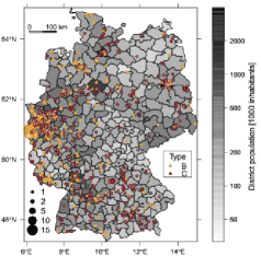
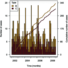
(a) Spatial point pattern with dot size	(b) Monthly aggregated time series and
proportional to the number of cases at	evolution of the cumulative number of cases
the respective location (postcode level)	(by date of specimen sampling)

Figure 2: Distribution of the 635 IMD cases in Germany, 2002–2008, caused by the two most common meningococcal finetypes B:P1.7-2,4:F1-5 (335 cases) and C:P1.5,2:F3-3 (300 cases), as reported to and typed by the German Reference Centre for Meningococci.

Note that the distinction between two finetypes in this application actually corresponds to a marked version of the point process model. It is described by an intensity function $\lambda(t,\mathbf{s},k)$, where the sum in (1) is restricted to previously infected individuals with bacterial finetype $k$, since we assume that infections of different finetypes are not associated via transmission [Meyer, Elias and Höhle (2012)]. For convenience, we kept notation simple and comparable to the multivariate time-series model of Section 3.

Prior to fitting point process models to the IMD data, the interval-censored nature of the data caused by a restricted resolution in space and time has to be taken into account: we only observed dates and residence postcodes of the cases (implicitly assuming that infections effectively happened within the residential neighbourhood). This makes the data interval-censored, yielding tied observations. However, ties are not compatible with our (continuous-time, continuous-space) point process model since observing two events at the exact same time point or location has zero probability. In the original analyses with a Gaussian kernel $f$, events were untied in time by subtracting a $U(0,1)$-distributed random number from all observed time points [Meyer, Elias and Höhle (2012)], that is, random sampling within each day, which is also the preferred method used by Diggle, Kaimi and Abellana (2010). To identify the two-parameter power law $(x+\sigma)^{-d}$, it was additionally necessary to break ties in space, since otherwise $\log\sigma$ diverged to $-\infty$, yielding a pole at $x=0$. A possible solution is to shift all locations randomly in space within their round-off intervals similar to the tie-breaking in time. Lacking a shapefile of the postcode regions, we shifted locations by a vector uniformly drawn from the disc with radius $\varepsilon/2$, where $\varepsilon$ is the minimum observed spatial separation of distinct points, here $\varepsilon=1.17$ km. Accordingly, a sensitivity analysis was conducted by applying the random tie-breaking in time and space 30 times and fitting the models to all replicates.

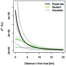
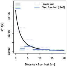
(a) Power laws vs. the Gaussian kernel	(b) Power law vs. a step function

Figure 3: Estimated spatial interaction functions—appropriately scaled by the epidemic intercept $\exp(\gamma_{0})$. The dashed lines represent 95% confidence intervals obtained as the pointwise 2.5% and 97.5% quantiles of the functions evaluated for 999 samples from the asymptotic multivariate normal distribution of the affected parameters. The light grey lines are estimates obtained from a sensitivity analysis with repeated random tie-breaking.

Table 1: Parameter estimates and 95% Wald confidence intervals for the Gaussian and the power-law model. Results for the Gaussian kernel are slightly different from those reported by Meyer, Elias and Höhle (2012) due to improved numerical integration. Note that we use the symbol $\sigma$ for the scale parameter and $d$ for the decay parameter in all spatial interaction functions, but these parameters as well as $\gamma_{0}$ are not directly comparable (instead see Figure 3)

	Gaussian kernel (2)		Power-law kernel (3)
	Estimate	95% CI	Estimate	95% CI
$\beta_{0}$	$-20.53$	${-}20.62\mbox{ to }{-}20.44$	$-20.58$	${-}20.68\mbox{ to }{-}20.47$
$\beta_{\mathrm{trend}}$	$-0.05$	${-}0.09\mbox{ to }{-}0.00$	$-0.05$	${-}0.09\mbox{ to }0.00$
$\beta_{\sin}$	$0.26$	$0.14\mbox{ to }0.39$	$0.26$	$0.12\mbox{ to }0.39$
$\beta_{\cos}$	$0.26$	$0.14\mbox{ to }0.39$	$0.27$	$0.14\mbox{ to }0.40$
$\gamma_{0}$	$-12.53$	${-}13.15\mbox{ to }{-}11.91$	$-6.21$	${-}9.32\mbox{ to }{-}3.10$
$\gamma_{\mathrm{C}}$	$-0.91$	${-}1.44\mbox{ to }{-}0.39$	$-0.80$	${-}1.31\mbox{ to }{-}0.29$
$\gamma_{3{-}18}$	$0.67$	$0.04\mbox{ to }1.31$	$0.78$	$0.11\mbox{ to }1.45$
$\gamma_{\geq 19}$	$-0.29$	${-}1.19\mbox{ to }0.61$	$-0.18$	${-}1.11\mbox{ to }0.75$
$\sigma$	$16.37$	$13.95\mbox{ to }19.21$	$4.60$	$1.80\mbox{ to }11.71$
$d$			$2.47$	$1.80\mbox{ to }3.39$

Figure 3(a) displays estimated spatial interaction functions—appropriately scaled by $\exp(\hat{\gamma}_{0})$—together with confidence intervals and estimates from the sensitivity analysis (see Table 1 for values of $\hat{\gamma}_{0}$, $\hat{\sigma}$, and $\hat{d}$). The power law puts much more weight on localised transmissions with an initially faster distance decay of infectivity. Furthermore, it features a heavier tail than the Gaussian kernel, which facilitates the geographical spread of IMD by occasional long-range transmissions. Maps of the accumulated epidemic intensity [Meyer and Held (2014), Figure 1] visualise the impact of the power law on the modelled infectivity. Sensitivity analysis shows that AIC clearly prefers the new power-law kernel against the Gaussian kernel (mean $\Delta\operatorname{AIC}=-27.6$, $\mathrm{SD}=1.5$). The Student kernel represents a compromise between the other two parametric kernels with short-range properties similar to the Gaussian kernel but with a heavy tail. However, AIC improvement is not as large as for the above power law (mean $\Delta\operatorname{AIC}=-15.5$, $\mathrm{SD}=0.9$).

For these three kernels, sensitivity analysis of the random tie-breaking procedure in space and time generally confirmed the results. The Gaussian kernel was least affected by the small-scale perturbation of event times and locations. Some replicates for the power-law model yielded a slightly steeper shape, which is due to closely located points after random tie-breaking. Such an artifact would have been avoided if we had used constrained sampling in that the randomly shifted points obey a minimum separation of say 0.1 km.

The estimated lagged version of the power law (4) is shown in Supplement B [Meyer and Held (2014), Figure 2]. It has a uniform short-range dispersal radius of $\hat{\sigma}=0.40$ (95% CI: 0.18 to 0.86) kilometres. However, such a small $\sigma$ is not interpretable since it is actually not covered by the spatial resolution of the data. Accordingly, the 30 estimates of the sensitivity analysis are more dispersed, as is the goodness of fit compared to the Gaussian kernel (mean $\Delta\operatorname{AIC}=-21.1$, $\mathrm{SD}=3.8$).

Figure 3(b) shows a comparison of the estimated power law with a step function (6) for spatial interaction. An upper boundary knot had to be specified, which we set at 100 kilometres, where the step function drops to 0. We chose six knots to be equidistant on the log-scale within $[0,\log(100)]$, that is, steps at 1.9, 3.7, 7.2, 13.9, 26.8, and 51.8 kilometres. Estimation took only 72 seconds due to the analytical implementation of the integration of $f_{2}$ over polygonal domains, whereas the power-law model took 42 minutes. The power law is well confirmed by the step function; it is almost completely enclosed by its 95% confidence interval. The step function suggests an even steeper initial decay and has a slightly better fit in terms of AIC (mean $\Delta\operatorname{AIC}=-6.9$, $\mathrm{SD}=4.0$ compared to the power law). However, it depends on the choice of knots, it is sensitive for artifacts of the data and forfeits monotonicity, which contradicts Tobler’s first law of geography [Tobler (1970)].

Parameter estimates and confidence intervals for the Gaussian and the power-law model are presented in Table 1 [see Meyer and Held (2014), Table 1, for parameter estimates of the other models]. The parameters of the endemic component characterising time trend and seasonality were not affected by the change of the shape of spatial interaction, and also the epidemic coefficients of finetype and age group do not differ much between the models retaining their signs and orders of magnitude. For instance, also with the power-law kernel, the C-type is approximately half as infectious as the B-type, which is estimated by the multiplicative type-effect $\exp(\hat{\gamma}_{\mathrm{C}})=0.45$ (95% CI: 0.27 to 0.75) on the force of infection (type B is the reference category here).

An important quantity in epidemic modelling is the expected number $R$ of offspring (secondary infections) each case generates. This reproduction number can be derived from the fitted models for each event by integrating its triggering function $\eta_{j}g(t-t_{j})f(\|\mathbf{s}-\mathbf{s}_{j}\|)$ over the observation region $\mathbf{W}$ and period $[t_{j},T]$ [Meyer, Elias and Höhle (2012)]. Type-specific estimates of $R$ are then obtained by averaging over the individual estimates by finetype. Table 2 shows that the reproduction numbers become slightly larger, which is related to the heavier tail of the power law enabling additional interaction between events at far distances.

Table 2: Type-specific reproduction numbers with 95% confidence intervals (based on 199 samples from the asymptotic multivariate normal distribution of the parameter estimates)

	Gaussian kernel (2)		Power-law kernel (3)
	Estimate	95% CI	Estimate	95% CI
B	0.22	0.17 to 0.31	0.26	0.10 to 0.35
C	0.10	0.06 to 0.15	0.13	0.05 to 0.19

We close this application with two additional ideas for improvement of the model. First, it might be worth considering a population effect also in the epidemic component to reflect higher contact rates and thus infectivity in regions with a denser population. Using the log-population density of the infective’s district, $\log\rho_{[t_{j}][\mathbf{s}_{j}]}$, the corresponding parameter is estimated to be $\hat{\gamma}_{\log(\rho)}=0.21$ (95% CI: $-$0.07 to 0.48), that is, individual infectivity scales with $\rho^{0.21}$, where $\rho$ ranges from 39 to 4225 km². Although the positive point estimate supports this idea, the wide confidence interval does not reflect strong evidence for such a population effect in the IMD data.

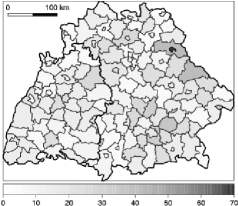
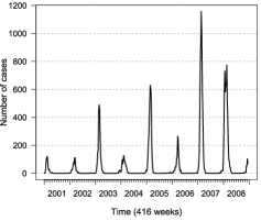
(a) Mean yearly incidence per 100,000	(b) Weekly number of cases
inhabitants

Figure 4: Spatial and temporal distribution of reported influenza cases in the 140 districts of Bavaria and Baden-Württemberg during the years 2001 to 2008.

However, it is helpful to allow for spatial heterogeneity in the endemic component. For instance, an indicator for districts at the border or the distance of the district’s centroids from the border could serve as proxies for simple edge effects. The idea is that as we get closer to the edge of the observation window (Germany) more infections will originate from external sources not directly linked to the observed history of the epidemic within Germany. We thus model a spatially varying risk of importing cases through the endemic component. For the Greater Aachen Region in the central-west part of Germany, where a spatial disease cluster is apparent in Figure 2(a), such a cross-border effect with the Netherlands was indeed identified by Elias et al. (2010) for the serogroup B finetype during our observation period using molecular sequence typing of bacterial strains in infected patients from both countries. Inclusion of an edge indicator in the endemic covariates $\mathbf{z}_{[t][\mathbf{s}]}$ improves AIC by 5 with an estimated rate ratio of 1.37 (95% CI: 1.10 to 1.70) for districts at the border versus inner districts. If we instead use the distance to the border, AIC improves by 20 with an estimated risk reduction of 5.0% (95% CI: 3.0% to 7.0%) per 10 km increase in distance to the border.

4.2 Influenza surveillance data from Southern Germany, 2001–2008 (see Figure 4)

The best model (with respect to logS and RPS) for the influenza surveillance data found by Held and Paul (2012) using normalised first-order weights included $S=1$ sinusoidal wave in each of the autoregressive ($\lambda_{it}$) and spatio-temporal ($\phi_{it}$) components and $S=3$ harmonic waves with a linear trend in the endemic component $\nu_{it}$ with the population fraction $e_{i}$ in region $i$ as offset. We now fit an extended model by estimating (raw or normalised) power-law neighbourhood weights (9) or (10) as described in Section 3.2, which replace the previously used fixed adjacency indicator.

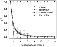
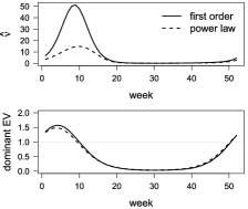
(a) Power-law (10) and unconstrained	(b) Seasonal variation of the endemic (top)
weights (11) with 95% confidence intervals	and epidemic (bottom) components

Figure 5: Estimated power-law and unconstrained weights (a), and seasonal variation (b) using normalised weights.

Figure 5(a) shows the estimated normalised power law with $\hat{d}=1.80$ (95% CI: 1.61 to 2.01). This decay is remarkably close to the power-law exponent 1.59 estimated by Brockmann, Hufnagel and Geisel (2006) for short-time travel in the USA with respect to distance (in kilometres), even though neighbourhood order is a discretised measure with no one-to-one correspondence to Euclidean distances, and travel behaviour in the USA is potentially different from that in Southern Germany. The plot also shows the estimated unconstrained weights for comparison with the power law. The sixth order of neighbourhood was the highest for which we could estimate an individual weight; higher orders had to be aggregated corresponding to $M=7$ in (11). The unconstrained weights decrease monotonically and resemble nicely the estimated power law, which is enclosed by the 95% confidence intervals (except for order 5, which has a slightly higher weight). The results with raw weights are very similar and shown in Meyer and Held [(2014), Figure 3].

Figure 5(b) shows the estimated seasonal variation in the endemic component and the course of the dominant eigenvalue [Held and Paul (2012)] for the normalised weight models. The dominant eigenvalue is a combination of the two epidemic components: if it is smaller than 1, it can be interpreted as the epidemic proportion of total disease incidence, otherwise it indicates an outbreak period. Whereas the course of this combined measure is more or less unchanged upon accounting for higher-order neighbours with a power law, the weight of the endemic component decreases remarkably. This goes hand in hand with an increased importance of the spatio-temporal component since in the power-law formulation much more information can be borrowed from the number of cases in other regions. Jumps of the epidemic to nonadjacent regions within one week are no longer dedicated to the endemic component only.

Concerning the remaining coefficients, there is less overdispersion in the power-law models (see $\psi$ in Table 3), which indicates reduced residual heterogeneity. For the variance and correlation estimates of the random effects, there is no substantial difference between first-order and power-law models and even less between raw and normalised formulations.

Table 3: Estimated model parameters (with standard errors) excluding intercepts and trend/seasonal coefficients. The parameter $\beta^{(\phi)}_{\mathrm{log(pop)}}$ in the first row belongs to a further extended power-law (PL) model, which accounts for population in the spatio-temporal component (last column). The $\sigma^{2}_{\cdot}$ and $\rho_{\cdot\cdot}$ parameters are the variances and correlations of the random effects (from $\bolds{\Sigma}$). The last row shows the final values of the penalised and marginal log-likelihoods

	Raw weights		Normalised weights
	First order	Power law	First order	Power law	PL$\bolds{{}+{}}$pop.
${\beta}^{(\phi)}_{\mathrm{log(pop)}}$	–	–	–	–	0.76 (0.13)
${d}$	–	1.72 (0.10)	–	1.80 (0.10)	1.65 (0.10)
${\psi}$	0.93 (0.03)	0.86 (0.03)	0.92 (0.03)	0.86 (0.03)	0.86 (0.03)
${\sigma}^{2}_{\lambda}$	0.14	0.17	0.13	0.17	0.16
${\sigma}^{2}_{\phi}$	0.94	0.92	0.98	0.89	0.71
${\sigma}^{2}_{\nu}$	0.50	0.67	0.51	0.67	0.66
${\rho}_{\lambda\phi}$	0.02	0.20	0.03	0.21	0.13
${\rho}_{\lambda\nu}$	0.11	0.31	0.12	0.31	0.27
${\rho}_{\phi\nu}$	0.56	0.29	0.55	0.30	0.39
$l_{\mathrm{pen}}(l_{\mathrm{mar}})$	$-$18,400 ($-$433)	$-$18,129 ($-$456)	$-$18,387 ($-$436)	$-$18,124 ($-$453)	$-$18,124 ($-$439)

To assess if the power-law formulation improves the previous first-order model, their predictive performance is compared based on one-week-ahead predictions for all 140 regions and the 104 weeks of the last two years. Computing these predictions for one model takes about 3 hours, since it needs to be refitted for every time point. Table 4 shows the resulting mean scores with associated $p$-values. Both logS and RPS improve when accounting for higher-order neighbours with a power law, while the difference is only significant for the logarithmic score. Furthermore, the normalised formulation performs slightly better than the raw weights. For instance, the mean difference in the logarithmic scores of the respective power-law models has an associated $p$-value of 0.0009. In the following we therefore only consider the normalised versions. For additional comparison, the simple uniform weight model ($w_{ji}\equiv 1$), which takes into account higher-order neighbours but with equal weight, has mean $\operatorname{logS}=0.5484$ and mean $\operatorname{RPS}=0.4215$, and thus performs worse than a power-law decay and, according to the RPS, even worse than first-order weights.

Table 4: Mean scores of $104\times 140$ one-week-ahead predictions over the last two years, accompanied with $p$-values for comparing power-law and first-order weights obtained via permutation tests with 19,999 random permutations. Note that the values obtained for normalised first-order weights are slightly different from the ones published by Held and Paul (2012) due to a correction of a recording error in the last week of the influenza data

	Raw weights		Normalised weights
	logS	RPS	logS	RPS
First order	0.55220	0.4205	0.5511	0.4194
Power law	0.54530	0.4174	0.5448	0.4168
$p$-value	0.00005	0.1100	0.0001	0.1900

Similarly to the IMD analysis, further improvement of the model’s description of human mobility can be achieved by accounting for the district-specific population also in the spatio-temporal component. The idea is that there tends to be more traffic to regional conurbations, that is, districts with a larger population, which are thus expected to import a bigger amount of cases from neighbouring regions [Bartlett (1957)]. Note that inclusion of the log-population in $\mathbf{z}^{(\phi)}_{it}$ affects susceptibility rather than infectivity, which is inverse to modelling the force of infection in the individual-based framework. The influenza data yield an estimated coefficient of $\hat{\beta}^{(\phi)}_{\mathrm{log(pop)}}=0.76$ (95% CI: 0.50 to 1.01), which provides strong evidence for such an agglomeration effect. The variance of the random effect $b_{i}^{(\phi)}$ of the spatio-temporal component is slightly reduced from 0.89 to 0.71, reflecting a decrease in residual heterogeneity between districts. The decay parameter is estimated to be slightly smaller in the extended model [$\hat{d}=1.65$ (95% CI: 1.45 to 1.86)] and all other effects remain approximately unchanged (see Table 3). However, the predictive performance improves only minimally, for example, the logarithmic score decreases from 0.5448 to 0.5447 ($p=0.66$). This small change could be related to the random effects $b_{i}^{(\phi)}$, which replace parts of the population effect if it is not included as a covariate. Indeed, there is correlation ($r_{\mathrm{Pearson}}=0.41$) between log(pop_i) and $b_{i}^{(\phi)}$ in the model without an explicit population effect in $\phi_{it}$ [see the scatterplot in Meyer and Held (2014), Figure 5].

4.3 Long-term forecast of the 2008 influenza wave

For further evaluation of the power-law models described in Section 4.2, we carry out a long-term forecast of the wave of influenza in 2008. Specifically, we simulate the evolution of the epidemic during the first 20 weeks in 2008 for each model trained by the previous years and initialised by the 18 cases of the last week of 2007 (see the animation in Supplement A, for their spatial distribution). Predictive performance is then evaluated by the final size distributions and by proper scoring rules assessing the empirical distributions induced by the simulated counts both in the temporal and spatial domains. Since the logarithmic score is infinite in the case of zero predictive probability for the observed count, we instead use the Dawid and Sebastiani (1999) score

$$\operatorname{DSS}(P,y)=\frac{(y-\mu_{P})^{2}}{\sigma_{P}^{2}}+\log\sigma_{P}^{2},$$

where $\mu_{P}$ and $\sigma_{P}^{2}$ denote the mean and the variance of $P$ [see also Gneiting and Raftery (2007)].

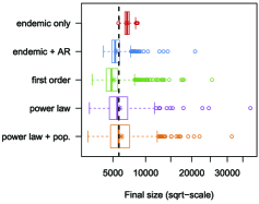
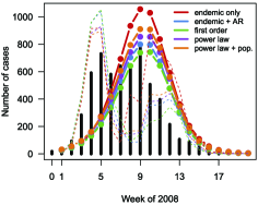
(a) Final size distributions ($\sqrt{}$-scale). The	(b) Time series of observed (bars) and mean
star in each box represents the mean, and	simulated (dots) counts aggregated over all
the vertical dashed line marks the	districts. Week 0 corresponds to the initial
observed final size of 5781 cases	condition (2007-W52). The dashed lines show
	the (scaled) RPS (see also Table 5)

Figure 6: Summary statistics of 1000 simulations of the wave of influenza during the first 20 weeks of 2008 for five competing models.

Table 5: Long-term predictive performance of 5 competing models in the temporal and spatial dimensions measured by mean DSS and RPS for the 2008 wave of influenza

Model	Time		Space		Space–time
	DSS	RPS	DSS	RPS	DSS	RPS
Endemic only	27.03	149.77	7.85	15.39	2.91	1.31
Endemic${}+{}$autoregressive	31.36	112.15	7.59	15.04	2.58	1.26
First order	26.46	108.61	7.51	15.63	2.50	1.26
Power law	16.41	110.20	7.36	14.75	2.29	1.25
Power law${}+{}$population	15.49	111.86	7.24	14.30	2.29	1.24

Figure 6(a) shows the final size distributions of the simulated waves of influenza during the first 20 weeks of 2008. Note that model complexity increases from top to bottom and that we also considered the naive endemic model, that is, independent counts, and the model without a spatio-temporal component as additional benchmarks. The endemic-only model, which decomposes disease incidence into spatial variation across districts, a seasonal and a log-linear time trend, overestimates the reported size of 5781 cases. It also does not allow for much variability in the size of the outbreak as opposed to the models with epidemic potential. The power-law models show the greatest amount of variation but best meet the reported final size: the power-law model without the population effect yields a simulated mean of 6022 (95% CI: 3126 to 10,808). The huge uncertainty seems plausible with regard to the long forecast horizon over a whole epidemic wave.

Figure 6(b) shows the time series of observed and mean simulated counts aggregated over all districts. In 2008, the wave grew two or more weeks earlier than in previous years trained by the sinusoidal terms in the three components. This phenomenon cannot be captured by the simulations, which are solely based on the observed pattern during 2001–2007 and the distribution of the cases from the last week of 2007. Furthermore, instead of two peaks as observed specifically in 2008, the simulations yield a single, larger peak where the power-law models on average induce the best amplitudes with respect to final size. The simulated spatial distribution of the cases (see Figure 7) is very similar among the various models and agrees quite well with the observed pattern. Animations of the observed and mean simulated epidemics provide more insight about the epidemic spread and are available in Supplement A. It is difficult to see a clear-cut traveling-wave of influenza in the reported data, which suggests that both an endemic component capturing immigration as well as scale-free jumps via the spatio-temporal component, that is, power-law weights $w_{ji}$, are important. Supplement A also includes an animated series of weekly probability integral transform (PIT) histograms [Gneiting, Balabdaoui and Raftery (2007)] using the nonrandomised version for count data proposed by Czado, Gneiting and Held (2009). These sequential PIT histograms mainly reflect the above time shift of the predictions. More clearly than the plots, the mean scores in Table 5 show that predictive performance generally improves with increasing model complexity and use of a power-law decay.

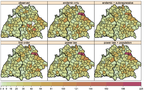
Figure 7: Observed and mean simulated incidence (cases per 100 000 inhabitants) aggregated over the 20 weeks forecast horizon (see Figure 6 of Supplement B for scatterplots).

5 Discussion

Motivated by the finding of Brockmann, Hufnagel and Geisel (2006) that short-time human travel roughly follows a power law with respect to distance, we investigated a power-law decay of spatial dependence between infections in two modelling frameworks for spatio-temporal surveillance data. A spatio-temporal point process model was applied to case reports of invasive meningococcal disease, and a multivariate time-series model was applied to counts of influenza aggregated by week and district. Since human mobility is an important driver of epidemic spread, the aim was to improve the predictive performance of these models using a power-law transmission kernel with respect to distance or neighbourhood order, respectively, where the decay is estimated jointly with all other model parameters.

In both applications considered, the power-law formulations performed better than previously used naive Gaussian or first-order interaction models, respectively. Furthermore, alternative piecewise constant, but otherwise unrestricted interaction models were in line with the estimated power laws. This confirms that the power-law distribution of short-time human travel translates to the modelling of infectious disease spread. We note that the qualitative interaction models could be replaced by (cubic) smoothing spline formulations, either in a continuous [Eubank (2000)] or in discrete fashion [Fahrmeir and Knorr-Held (2000)]. In order to penalise deviations from the power law, this should be done on a log–log scale, where the power law is a simple linear relationship. However, data-driven estimation of the smoothing parameter may become difficult.

The heavy tail of the power law allows for long-range dependence between cases, which accordingly increased the importance of the epidemic component in both models. An alternative formulation of spatial interaction with occasional long-range transmission was used by Diggle (2006), who added a small distance-independent value to a powered exponential term of the scaled distance. However, this offset and the power parameter are poorly identified. For the 2001 UK foot-and-mouth disease epidemic, Keeling et al. (2001) observed a power-law-like, sharply peaked transmission kernel, and Chis Ster and Ferguson (2007) subsequently found that the power law (3) yields a much better fit than the offset kernel or other functional forms, which is in accordance with our results for the spread of human infectious diseases.

Regions at the edge of the observation window are missing potential sources of infection from the unobserved side of the border. To capture unobserved heterogeneity due to immigration/edge effects, the count data model includes region-specific random effects $b_{i}^{(\nu)}$ in the endemic component. However, there was no clear pattern in their estimates with respect to regions being close to the border or not [Meyer and Held (2014), Figure 4]. In contrast, the IMD data supported edge effects, specifically concerning the border to the Netherlands. The spatial occurrence of cases met our simplistic approach of including the distance to the border as a covariate in the endemic component. This ignores that immigration might be more important in large metropolitan areas attracting people from abroad regardless of the location within Germany. A better way of accounting for edge effects would thus be to explicitly incorporate immigration data. For instance, Geilhufe et al. (2014) used incoming road or air traffic from outside North Norway as a proxy for the risk of importing cases of influenza, which led to improved predictive performance while also accounting for population in the spatio-temporal component.

Scaling regional susceptibility by population size proved very informative also for influenza in Southern Germany: more populated regions seem to attract more infections from neighbours than smaller regions, which reflects commuter-type imports [see Viboud et al. (2006), and Keeling and Rohani (2008), Section 6.3.3.1]. An exception of such a population effect in the spatio-temporal component might be seasonal accumulations in low-populated touristic regions. In the point process model for the IMD cases, the effect of population density on infectivity was less evident, which might be related to the very limited size of the point pattern with less than 100 cases per year over all of Germany.

Another limitation of the IMD data set is tied locations of cases due to censoring at the postcode level. For the power law to be identifiable, we randomly sampled the locations from discs of radius 0.59 km around the centroid of the respective postcode area, and verified that our results are insensitive to the random seed. Note that choosing a larger radius of, for example, 3 km, leads to less pronounced weight towards zero distance but yields otherwise similar results, especially concerning the relative performance of the various interaction functions.

We considered power laws as a description of spatial dispersal of infectious diseases as motivated by human travelling behaviour. Concerning temporal dispersal, power laws are usually not an appropriate description of the evolution of infectivity over time. Infectious diseases typically feature a very limited period of infectivity after the incubation period, since an infected individual will receive treatment and typically restrict its interaction radius upon the appearance of symptoms. Due to the small number of cases in the IMD data, we could not estimate a parametric temporal interaction function $g(t)$ and simply assumed constant infectivity during 30 days as in Meyer, Elias and Höhle (2012). More generally, $g(t)$ could represent an increasing level of infectivity beginning from exposure, followed by a plateau and then decreasing and eventually vanishing infectivity [Lawson and Leimich (2000), Section 5.3]. In the multivariate time-series model, the counts were restricted to only explicitly depend on the previous week. This is reasonable if the generation time, the time consumed by an infective to cause a secondary case, is not larger than the aggregation time in the surveillance data. For human influenza, Cowling et al. (2009) report a mean generation time of 3.6 days (95% CI: 2.9 days to 4.3 days).

Long-term simulated forecast of the 2008 influenza wave confirmed that the power-law model yields better predictions. However, the model was not able to describe the onset in 2008, which was two weeks earlier than in the years 2001–2007. For this to work, it would be necessary to further enrich the model by external processes such as vaccination coverage [as in Herzog, Paul and Held (2011)] or climate conditions [Fuhrmann (2010), Willem et al. (2012)] entering as covariates in the endemic and/or epidemic components. An alternative approach has been used by Fanshawe et al. (2008), where seasonality parameters were allowed to change from year to year according to a random walk model. Implementation would then require Markov chain Monte Carlo or other more demanding techniques for inference. Despite the open issue of dynamic seasonality, the simulated final size and spatial distribution matched the reported epidemic quite well.

This success also suggests that under-reporting of influenza was roughly constant over time. For instance, the 4 districts which did not report any cases during the 2008 forecast period (SK Kempten, SK Memmingen, LK Kelheim, and SK Aschaffenburg) only reported 1, 0, 20, and 4 cases in total during 2001–2007. However, we can only model the effectively reported number of cases, which may be affected by time-varying attention drawn to influenza in the media. Syndromic surveillance systems aim to unify various routinely collected data sources, for example, web searches for outbreak detection and monitoring [Josseran et al. (2006), Hulth, Rydevik and Linde (2009)], and may thereby provide a more realistic picture of influenza.

Prospective detection of outbreaks is also possible based on the count data model presented here. A statistic could be based on quantiles of the distribution of $Y_{i,t+1}|\mathbf{Y}_{\cdot,t}$, for example, an alarm could be triggered if the actual observed counts at $t+1$ are above the 99% quantile, say, [Held et al. (2006)]. Note that by including seasonality in the model, a yearly wave at the beginning of the year would be ‘planned’ and not necessarily considered a deviation from default behaviour.

Our power-law approach is very useful in the absence of movement network data (e.g., plane and train traffic). However, if such data were available [Lazer et al. (2009)], neighbourhood weights $w_{ji}$ in the count data model could instead be based on the connectivity between regions, which was investigated by Schrödle, Held and Rue (2012) for the spread of Coxiellosis in Swiss cows and by Geilhufe et al. (2014) for the spread of influenza in Northern Norway. In recent work, Brockmann and Helbing (2013) introduce the ‘effective distance’ to describe the 2009 H1N1 influenza pandemic. Their approach relates to what has already been termed ‘functional distance’ by Brown and Horton (1970), that is, a function of (inter-)regional properties like population and commuter or travel flows such that it “reflects the net effect of entity properties upon the propensity of the entities to interact” [Brown and Holmes (1971)]. A recent example of using telephone call data as a measure of human interaction can be found in Ratti et al. (2010). Another fruitful area of future research is the statistical analysis of age-stratified surveillance data. Contact patterns vary across age [Mossong et al. (2008), Truscott et al. (2012)], calling for a unified analysis across age groups and regions.

Appendix: Software

All calculations have been carried out in the statistical software environment R 3.0.2 [R Core Team (2013)]. Both model frameworks and their power-law extensions presented in this paper are implemented in the R package surveillance [Höhle, Meyer and Paul (2014)] as of version 1.6-0 available from the Comprehensive R Archive Network (CRAN.R-project.org). The two analysed data sets are included therein as data("imdepi") (courtesy of the German Reference Centre for Meningococci) and data("fluBYBW") [raw data obtained from the German national surveillance system operated by the Robert Koch Institute (2009)]. The point process model (1) for individual point-referenced data can be fitted by the function twinstim(), and the multivariate time-series model (7) for count data is estimated by hhh4(). The implementations are flexible enough to allow for other specifications of the spatial interaction function $f$ and the weights $w_{ji}$, respectively. A related two-component epidemic model [Höhle (2009)], which is designed for time-continuous individual surveillance data of a closed population with a fixed set of locations, for example, for farm- or household-based epidemics, is also included as function twinSIR(). The application of all three model frameworks in R is described in detail in Meyer, Held and Höhle (2014).

Spatial integrals in the point process likelihood have been evaluated using cubature methods implemented in the R package polyCub 0.4-3 [Meyer (2014)]. Maps have been produced using sp 1.0-15 [Bivand, Pebesma and Gómez-Rubio (2013)] and animations using animation 2.2 [Xie (2013)].

References

- Albert and Barabási (2002) {barticle}[mr] \bauthor\bsnmAlbert, \bfnmRéka\binitsR. and \bauthor\bsnmBarabási, \bfnmAlbert-László\binitsA.-L. (\byear2002). \btitleStatistical mechanics of complex networks. \bjournalRev. Modern Phys. \bvolume74 \bpages47–97. \biddoi=10.1103/RevModPhys.74.47, issn=0034-6861, mr=1895096 \bptokimsref\endbibitem
- Bartlett (1957) {barticle}[author] \bauthor\bsnmBartlett, \bfnmM. S.\binitsM. S. (\byear1957). \btitleMeasles periodicity and community size. \bjournalJ. Roy. Statist. Soc. Ser. A \bvolume120 \bpages48–70. \bptokimsref\endbibitem
- Bivand, Pebesma and Gómez-Rubio (2013) {bbook}[mr] \bauthor\bsnmBivand, \bfnmRoger S.\binitsR. S., \bauthor\bsnmPebesma, \bfnmEdzer\binitsE. and \bauthor\bsnmGómez-Rubio, \bfnmVirgilio\binitsV. (\byear2013). \btitleApplied Spatial Data Analysis with R, \bedition2nd ed. \bseriesUse R! \bvolume10. \bpublisherSpringer, \blocationNew York. \biddoi=10.1007/978-1-4614-7618-4, mr=3099410 \bptokimsref\endbibitem
- Brockmann and Helbing (2013) {barticle}[pbm] \bauthor\bsnmBrockmann, \bfnmDirk\binitsD. and \bauthor\bsnmHelbing, \bfnmDirk\binitsD. (\byear2013). \btitleThe hidden geometry of complex, network-driven contagion phenomena. \bjournalScience \bvolume342 \bpages1337–1342. \biddoi=10.1126/science.1245200, issn=1095-9203, pii=342/6164/1337, pmid=24337289 \bptokimsref\endbibitem
- Brockmann, Hufnagel and Geisel (2006) {barticle}[pbm] \bauthor\bsnmBrockmann, \bfnmD.\binitsD., \bauthor\bsnmHufnagel, \bfnmL.\binitsL. and \bauthor\bsnmGeisel, \bfnmT.\binitsT. (\byear2006). \btitleThe scaling laws of human travel. \bjournalNature \bvolume439 \bpages462–465. \biddoi=10.1038/nature04292, issn=1476-4687, pii=nature04292, pmid=16437114 \bptokimsref\endbibitem
- Brown and Holmes (1971) {barticle}[author] \bauthor\bsnmBrown, \bfnmLawrence A.\binitsL. A. and \bauthor\bsnmHolmes, \bfnmJohn\binitsJ. (\byear1971). \btitleThe delimitation of functional regions, nodal regions, and hierarchies by functional distance approaches. \bjournalJ. Reg. Sci. \bvolume11 \bpages57–72. \bptokimsref\endbibitem
- Brown and Horton (1970) {barticle}[author] \bauthor\bsnmBrown, \bfnmLawrence A.\binitsL. A. and \bauthor\bsnmHorton, \bfnmFrank E.\binitsF. E. (\byear1970). \btitleFunctional distance: An operational approach. \bjournalGeogr. Anal. \bvolume2 \bpages76–83. \bptokimsref\endbibitem
- Chilès and Delfiner (2012) {bbook}[mr] \bauthor\bsnmChilès, \bfnmJean-Paul\binitsJ.-P. and \bauthor\bsnmDelfiner, \bfnmPierre\binitsP. (\byear2012). \btitleGeostatistics: Modeling Spatial Uncertainty, \bedition2nd ed. \bseriesWiley Series in Probability and Statistics \bvolume713. \bpublisherWiley, \blocationHoboken, NJ. \biddoi=10.1002/9781118136188, mr=2850475 \bptokimsref\endbibitem
- Chis Ster and Ferguson (2007) {barticle}[pbm] \bauthor\bsnmChis Ster, \bfnmIrina\binitsI. and \bauthor\bsnmFerguson, \bfnmNeil M.\binitsN. M. (\byear2007). \btitleTransmission parameters of the 2001 foot and mouth epidemic in Great Britain. \bjournalPLoS ONE \bvolume2 \bpagese502. \biddoi=10.1371/journal.pone.0000502, issn=1932-6203, pmcid=1876810, pmid=17551582 \bptokimsref\endbibitem
- Cowling et al. (2009) {barticle}[author] \bauthor\bsnmCowling, \bfnmBenjamin J.\binitsB. J., \bauthor\bsnmFang, \bfnmVicky J.\binitsV. J., \bauthor\bsnmRiley, \bfnmSteven\binitsS., \bauthor\bsnmPeiris, \bfnmJoseph Malik Sriyal\binitsJ. M. S. and \bauthor\bsnmLeung, \bfnmGabriel M.\binitsG. M. (\byear2009). \btitleEstimation of the serial interval of influenza. \bjournalEpidemiology \bvolume20 \bpages344–347. \bptokimsref\endbibitem
- Czado, Gneiting and Held (2009) {barticle}[mr] \bauthor\bsnmCzado, \bfnmClaudia\binitsC., \bauthor\bsnmGneiting, \bfnmTilmann\binitsT. and \bauthor\bsnmHeld, \bfnmLeonhard\binitsL. (\byear2009). \btitlePredictive model assessment for count data. \bjournalBiometrics \bvolume65 \bpages1254–1261. \biddoi=10.1111/j.1541-0420.2009.01191.x, issn=0006-341X, mr=2756513 \bptokimsref\endbibitem
- Dawid and Sebastiani (1999) {barticle}[mr] \bauthor\bsnmDawid, \bfnmA. Philip\binitsA. P. and \bauthor\bsnmSebastiani, \bfnmPaola\binitsP. (\byear1999). \btitleCoherent dispersion criteria for optimal experimental design. \bjournalAnn. Statist. \bvolume27 \bpages65–81. \biddoi=10.1214/aos/1018031101, issn=0090-5364, mr=1701101 \bptokimsref\endbibitem
- Deardon et al. (2010) {barticle}[mr] \bauthor\bsnmDeardon, \bfnmRob\binitsR., \bauthor\bsnmBrooks, \bfnmStephen P.\binitsS. P., \bauthor\bsnmGrenfell, \bfnmBryan T.\binitsB. T., \bauthor\bsnmKeeling, \bfnmMatthew J.\binitsM. J., \bauthor\bsnmTildesley, \bfnmMichael J.\binitsM. J., \bauthor\bsnmSavill, \bfnmNicholas J.\binitsN. J., \bauthor\bsnmShaw, \bfnmDarren J.\binitsD. J. and \bauthor\bsnmWoolhouse, \bfnmMark E. J.\binitsM. E. J. (\byear2010). \btitleInference for individual-level models of infectious diseases in large populations. \bjournalStatist. Sinica \bvolume20 \bpages239–261. \bidissn=1017-0405, mr=2640693 \bptokimsref\endbibitem
- Diggle (2006) {barticle}[mr] \bauthor\bsnmDiggle, \bfnmPeter J.\binitsP. J. (\byear2006). \btitleSpatio-temporal point processes, partial likelihood, foot and mouth disease. \bjournalStat. Methods Med. Res. \bvolume15 \bpages325–336. \biddoi=10.1191/0962280206sm454oa, issn=0962-2802, mr=2242245 \bptokimsref\endbibitem
- Diggle (2007) {bincollection}[auto] \bauthor\bsnmDiggle, \bfnmPeter J.\binitsP. J. (\byear2007). \btitleSpatio-temporal point processes: Methods and applications. In \bbooktitleStatistical Methods for Spatio-Temporal Systems (\beditor\bfnmBärbel\binitsB. \bsnmFinkenstädt, \beditor\bfnmLeonhard\binitsL. \bsnmHeld and \beditor\bfnmValerie\binitsV. \bsnmIsham, eds.) \bpages1–45. \bpublisherChapman & Hall/CRC, \blocationBoca Raton, FL. \bptokimsref\endbibitem
- Diggle, Kaimi and Abellana (2010) {barticle}[mr] \bauthor\bsnmDiggle, \bfnmPeter J.\binitsP. J., \bauthor\bsnmKaimi, \bfnmIrene\binitsI. and \bauthor\bsnmAbellana, \bfnmRosa\binitsR. (\byear2010). \btitlePartial-likelihood analysis of spatio-temporal point-process data. \bjournalBiometrics \bvolume66 \bpages347–354. \biddoi=10.1111/j.1541-0420.2009.01304.x, issn=0006-341X, mr=2758814 \bptokimsref\endbibitem
- Elias et al. (2010) {barticle}[pbm] \bauthor\bsnmElias, \bfnmJohannes\binitsJ., \bauthor\bsnmSchouls, \bfnmLeo M.\binitsL. M., \bauthor\bsnmvan de Pol, \bfnmIngrid\binitsI., \bauthor\bsnmKeijzers, \bfnmWendy C.\binitsW. C., \bauthor\bsnmMartin, \bfnmDiana R.\binitsD. R., \bauthor\bsnmGlennie, \bfnmAnne\binitsA., \bauthor\bsnmOster, \bfnmPhilipp\binitsP., \bauthor\bsnmFrosch, \bfnmMatthias\binitsM., \bauthor\bsnmVogel, \bfnmUlrich\binitsU. and \bauthor\bsnmvan der Ende, \bfnmArie\binitsA. (\byear2010). \btitleVaccine preventability of meningococcal clone, Greater Aachen region, Germany. \bjournalEmerg. Infect. Dis. \bvolume16 \bpages465–472. \biddoi=10.3201/eid1603.091102, issn=1080-6059, pmcid=3322024, pmid=20202422 \bptokimsref\endbibitem
- Eubank (2000) {bincollection}[auto] \bauthor\bsnmEubank, \bfnmRandall L.\binitsR. L. (\byear2000). \btitleSpline regression. In \bbooktitleSmoothing and Regression: Approaches, Computation, and Application (\beditor\bfnmMichael G.\binitsM. G. \bsnmSchimek, ed.) \bpages1–18. \bpublisherWiley, \blocationNew York. \bptokimsref\endbibitem
- Fahrmeir and Knorr-Held (2000) {bincollection}[auto] \bauthor\bsnmFahrmeir, \bfnmLudwig\binitsL. and \bauthor\bsnmKnorr-Held, \bfnmLeonhard\binitsL. (\byear2000). \btitleDynamic and semiparametric models. In \bbooktitleSmoothing and Regression: Approaches, Computation, and Application (\beditor\bfnmMichael G.\binitsM. G. \bsnmSchimek, ed.) \bpages513–544. \bpublisherWiley, \blocationNew York. \bptokimsref\endbibitem
- Fanshawe et al. (2008) {barticle}[mr] \bauthor\bsnmFanshawe, \bfnmT. R.\binitsT. R., \bauthor\bsnmDiggle, \bfnmP. J.\binitsP. J., \bauthor\bsnmRushton, \bfnmS.\binitsS., \bauthor\bsnmSanderson, \bfnmR.\binitsR., \bauthor\bsnmLurz, \bfnmP. W. W.\binitsP. W. W., \bauthor\bsnmGlinianaia, \bfnmS. V.\binitsS. V., \bauthor\bsnmPearce, \bfnmM. S.\binitsM. S., \bauthor\bsnmParker, \bfnmL.\binitsL., \bauthor\bsnmCharlton, \bfnmM.\binitsM. and \bauthor\bsnmPless-Mulloli, \bfnmT.\binitsT. (\byear2008). \btitleModelling spatio-temporal variation in exposure to particulate matter: A two-stage approach. \bjournalEnvironmetrics \bvolume19 \bpages549–566. \biddoi=10.1002/env.889, issn=1180-4009, mr=2528540 \bptokimsref\endbibitem
- Farrington et al. (1996) {barticle}[mr] \bauthor\bsnmFarrington, \bfnmC. P.\binitsC. P., \bauthor\bsnmAndrews, \bfnmN. J.\binitsN. J., \bauthor\bsnmBeale, \bfnmA. D.\binitsA. D. and \bauthor\bsnmCatchpole, \bfnmM. A.\binitsM. A. (\byear1996). \btitleA statistical algorithm for the early detection of outbreaks of infectious disease. \bjournalJ. Roy. Statist. Soc. Ser. A \bvolume159 \bpages547–563. \biddoi=10.2307/2983331, issn=0964-1998, mr=1413665 \bptokimsref\endbibitem
- Fuhrmann (2010) {barticle}[author] \bauthor\bsnmFuhrmann, \bfnmChristopher\binitsC. (\byear2010). \btitleThe effects of weather and climate on the seasonality of influenza: What we know and what we need to know. \bjournalGeography Compass \bvolume4 \bpages718–730. \bptokimsref\endbibitem
- Geilhufe et al. (2014) {barticle}[author] \bauthor\bsnmGeilhufe, \bfnmMarc\binitsM., \bauthor\bsnmHeld, \bfnmLeonhard\binitsL., \bauthor\bsnmSkrøvseth, \bfnmStein Olav\binitsS. O., \bauthor\bsnmSimonsen, \bfnmGunnar S.\binitsG. S. and \bauthor\bsnmGodtliebsen, \bfnmFred\binitsF. (\byear2014). \btitlePower law approximations of movement network data for modeling infectious disease spread. \bjournalBiom. J. \bvolume56 \bpages363–382. \bptokimsref\endbibitem
- Gibson (1997) {barticle}[author] \bauthor\bsnmGibson, \bfnmGavin J.\binitsG. J. (\byear1997). \btitleMarkov chain Monte Carlo methods for fitting spatiotemporal stochastic models in plant epidemiology. \bjournalJ. R. Stat. Soc. Ser. C. Appl. Stat. \bvolume46 \bpages215–233. \bptokimsref\endbibitem
- Gneiting, Balabdaoui and Raftery (2007) {barticle}[mr] \bauthor\bsnmGneiting, \bfnmTilmann\binitsT., \bauthor\bsnmBalabdaoui, \bfnmFadoua\binitsF. and \bauthor\bsnmRaftery, \bfnmAdrian E.\binitsA. E. (\byear2007). \btitleProbabilistic forecasts, calibration and sharpness. \bjournalJ. R. Stat. Soc. Ser. B Stat. Methodol. \bvolume69 \bpages243–268. \biddoi=10.1111/j.1467-9868.2007.00587.x, issn=1369-7412, mr=2325275 \bptokimsref\endbibitem
- Gneiting and Raftery (2007) {barticle}[mr] \bauthor\bsnmGneiting, \bfnmTilmann\binitsT. and \bauthor\bsnmRaftery, \bfnmAdrian E.\binitsA. E. (\byear2007). \btitleStrictly proper scoring rules, prediction, and estimation. \bjournalJ. Amer. Statist. Assoc. \bvolume102 \bpages359–378. \biddoi=10.1198/016214506000001437, issn=0162-1459, mr=2345548 \bptokimsref\endbibitem
- Gneiting and Schlather (2004) {barticle}[mr] \bauthor\bsnmGneiting, \bfnmTilmann\binitsT. and \bauthor\bsnmSchlather, \bfnmMartin\binitsM. (\byear2004). \btitleStochastic models that separate fractal dimension and the Hurst effect. \bjournalSIAM Rev. \bvolume46 \bpages269–282 (electronic). \biddoi=10.1137/S0036144501394387, issn=0036-1445, mr=2114455 \bptokimsref\endbibitem
- Gutenberg and Richter (1944) {barticle}[author] \bauthor\bsnmGutenberg, \bfnmBeno\binitsB. and \bauthor\bsnmRichter, \bfnmCharles Francis\binitsC. F. (\byear1944). \btitleFrequency of earthquakes in California. \bjournalBull. Seismol. Soc. Amer. \bvolume34 \bpages185–188. \bptokimsref\endbibitem
- Hawkes (1971) {barticle}[mr] \bauthor\bsnmHawkes, \bfnmAlan G.\binitsA. G. (\byear1971). \btitleSpectra of some self-exciting and mutually exciting point processes. \bjournalBiometrika \bvolume58 \bpages83–90. \bidissn=0006-3444, mr=0278410 \bptokimsref\endbibitem
- Held, Höhle and Hofmann (2005) {barticle}[mr] \bauthor\bsnmHeld, \bfnmLeonhard\binitsL., \bauthor\bsnmHöhle, \bfnmMichael\binitsM. and \bauthor\bsnmHofmann, \bfnmMathias\binitsM. (\byear2005). \btitleA statistical framework for the analysis of multivariate infectious disease surveillance counts. \bjournalStat. Model. \bvolume5 \bpages187–199. \biddoi=10.1191/1471082X05st098oa, issn=1471-082X, mr=2210732 \bptokimsref\endbibitem
- Held and Paul (2012) {barticle}[mr] \bauthor\bsnmHeld, \bfnmLeonhard\binitsL. and \bauthor\bsnmPaul, \bfnmMichaela\binitsM. (\byear2012). \btitleModeling seasonality in space–time infectious disease surveillance data. \bjournalBiom. J. \bvolume54 \bpages824–843. \biddoi=10.1002/bimj.201200037, issn=0323-3847, mr=2993630 \bptokimsref\endbibitem
- Held et al. (2006) {barticle}[pbm] \bauthor\bsnmHeld, \bfnmLeonhard\binitsL., \bauthor\bsnmHofmann, \bfnmMathias\binitsM., \bauthor\bsnmHöhle, \bfnmMichael\binitsM. and \bauthor\bsnmSchmid, \bfnmVolker\binitsV. (\byear2006). \btitleA two-component model for counts of infectious diseases. \bjournalBiostatistics \bvolume7 \bpages422–437. \biddoi=10.1093/biostatistics/kxj016, issn=1465-4644, pii=kxj016, pmid=16407470 \bptokimsref\endbibitem
- Herzog, Paul and Held (2011) {barticle}[author] \bauthor\bsnmHerzog, \bfnmS. A.\binitsS. A., \bauthor\bsnmPaul, \bfnmMichaela\binitsM. and \bauthor\bsnmHeld, \bfnmLeonhard\binitsL. (\byear2011). \btitleHeterogeneity in vaccination coverage explains the size and occurrence of measles epidemics in German surveillance data. \bjournalEpidemiol. Infect. \bvolume139 \bpages505–515. \bptokimsref\endbibitem
- Höhle (2009) {barticle}[mr] \bauthor\bsnmHöhle, \bfnmMichael\binitsM. (\byear2009). \btitleAdditive-multiplicative regression models for spatio-temporal epidemics. \bjournalBiom. J. \bvolume51 \bpages961–978. \biddoi=10.1002/bimj.200900050, issn=0323-3847, mr=2744450 \bptokimsref\endbibitem
- Höhle, Meyer and Paul (2014) {bmisc}[author] \bauthor\bsnmHöhle, \bfnmMichael\binitsM., \bauthor\bsnmMeyer, \bfnmSebastian\binitsS. and \bauthor\bsnmPaul, \bfnmMichaela\binitsM. (\byear2014). \bhowpublishedsurveillance: Temporal and spatio-temporal modeling and monitoring of epidemic phenomena. R package version 1.8-0. \bptokimsref\endbibitem
- Höhle and Paul (2008) {barticle}[mr] \bauthor\bsnmHöhle, \bfnmMichael\binitsM. and \bauthor\bsnmPaul, \bfnmMichaela\binitsM. (\byear2008). \btitleCount data regression charts for the monitoring of surveillance time series. \bjournalComput. Statist. Data Anal. \bvolume52 \bpages4357–4368. \biddoi=10.1016/j.csda.2008.02.015, issn=0167-9473, mr=2432467 \bptokimsref\endbibitem
- Höhle, Paul and Held (2009) {barticle}[pbm] \bauthor\bsnmHöhle, \bfnmMichael\binitsM., \bauthor\bsnmPaul, \bfnmMichaela\binitsM. and \bauthor\bsnmHeld, \bfnmLeonhard\binitsL. (\byear2009). \btitleStatistical approaches to the monitoring and surveillance of infectious diseases for veterinary public health. \bjournalPrev. Vet. Med. \bvolume91 \bpages2–10. \biddoi=10.1016/j.prevetmed.2009.05.017, issn=1873-1716, pii=S0167-5877(09)00138-X, pmid=19539387 \bptokimsref\endbibitem
- Hulth, Rydevik and Linde (2009) {barticle}[pbm] \bauthor\bsnmHulth, \bfnmAnette\binitsA., \bauthor\bsnmRydevik, \bfnmGustaf\binitsG. and \bauthor\bsnmLinde, \bfnmAnnika\binitsA. (\byear2009). \btitleWeb queries as a source for syndromic surveillance. \bjournalPLoS ONE \bvolume4 \bpagese4378. \biddoi=10.1371/journal.pone.0004378, issn=1932-6203, pmcid=2634970, pmid=19197389 \bptokimsref\endbibitem
- Josseran et al. (2006) {barticle}[author] \bauthor\bsnmJosseran, \bfnmL.\binitsL., \bauthor\bsnmNicolau, \bfnmJ.\binitsJ., \bauthor\bsnmCaillère, \bfnmN.\binitsN., \bauthor\bsnmAstagneau, \bfnmP.\binitsP. and \bauthor\bsnmBrücker, \bfnmG.\binitsG. (\byear2006). \btitleSyndromic surveillance based on emergency department activity and crude mortality: Two examples. \bjournalEurosurveillance \bvolume11 \bpages225–229. \bptokimsref\endbibitem
- Keeling and Rohani (2002) {barticle}[author] \bauthor\bsnmKeeling, \bfnmMatt J.\binitsM. J. and \bauthor\bsnmRohani, \bfnmPejman\binitsP. (\byear2002). \btitleEstimating spatial coupling in epidemiological systems: A mechanistic approach. \bjournalEcol. Lett. \bvolume5 \bpages20–29. \bptokimsref\endbibitem
- Keeling and Rohani (2008) {bbook}[mr] \bauthor\bsnmKeeling, \bfnmMatt J.\binitsM. J. and \bauthor\bsnmRohani, \bfnmPejman\binitsP. (\byear2008). \btitleModeling Infectious Diseases in Humans and Animals. \bpublisherPrinceton Univ. Press, \blocationPrinceton, NJ. \bidmr=2354763 \bptokimsref\endbibitem
- Keeling et al. (2001) {barticle}[author] \bauthor\bsnmKeeling, \bfnmMatt J.\binitsM. J., \bauthor\bsnmWoolhouse, \bfnmMark E. J.\binitsM. E. J., \bauthor\bsnmShaw, \bfnmDarren J.\binitsD. J., \bauthor\bsnmMatthews, \bfnmLouise\binitsL., \bauthor\bsnmChase-Topping, \bfnmMargo\binitsM., \bauthor\bsnmHaydon, \bfnmDan T.\binitsD. T., \bauthor\bsnmCornell, \bfnmStephen J.\binitsS. J., \bauthor\bsnmKappey, \bfnmJens\binitsJ., \bauthor\bsnmWilesmith, \bfnmJohn\binitsJ. and \bauthor\bsnmGrenfell, \bfnmBryan T.\binitsB. T. (\byear2001). \btitleDynamics of the 2001 UK foot and mouth epidemic: Stochastic dispersal in a heterogeneous landscape. \bjournalScience \bvolume294 \bpages813–817. \bptokimsref\endbibitem
- Lawson and Leimich (2000) {barticle}[author] \bauthor\bsnmLawson, \bfnmAndrew B.\binitsA. B. and \bauthor\bsnmLeimich, \bfnmPetra\binitsP. (\byear2000). \btitleApproaches to the space–time modelling of infectious disease behaviour. \bjournalIMA J. Math. Appl. Med. Biol. \bvolume17 \bpages1–13. \bptokimsref\endbibitem
- Lazer et al. (2009) {barticle}[pbm] \bauthor\bsnmLazer, \bfnmDavid\binitsD., \bauthor\bsnmPentland, \bfnmAlex\binitsA., \bauthor\bsnmAdamic, \bfnmLada\binitsL., \bauthor\bsnmAral, \bfnmSinan\binitsS., \bauthor\bsnmBarabasi, \bfnmAlbert-Laszlo\binitsA.-L., \bauthor\bsnmBrewer, \bfnmDevon\binitsD., \bauthor\bsnmChristakis, \bfnmNicholas\binitsN., \bauthor\bsnmContractor, \bfnmNoshir\binitsN., \bauthor\bsnmFowler, \bfnmJames\binitsJ., \bauthor\bsnmGutmann, \bfnmMyron\binitsM., \bauthor\bsnmJebara, \bfnmTony\binitsT., \bauthor\bsnmKing, \bfnmGary\binitsG., \bauthor\bsnmMacy, \bfnmMichael\binitsM., \bauthor\bsnmRoy, \bfnmDeb\binitsD. and \bauthor\bsnmAlstyne, \bfnmMarshall Van\binitsM. V. (\byear2009). \btitleSocial science. Computational social science. \bjournalScience \bvolume323 \bpages721–723. \biddoi=10.1126/science.1167742, issn=1095-9203, mid=NIHMS98137, pii=323/5915/721, pmcid=2745217, pmid=19197046 \bptokimsref\endbibitem
- Le Comber et al. (2011) {barticle}[author] \bauthor\bsnmLe Comber, \bfnmSteven\binitsS., \bauthor\bsnmRossmo, \bfnmDarcy Kim\binitsD. K., \bauthor\bsnmHassan, \bfnmAli\binitsA., \bauthor\bsnmFuller, \bfnmDouglas\binitsD. and \bauthor\bsnmBeier, \bfnmJohn\binitsJ. (\byear2011). \btitleGeographic profiling as a novel spatial tool for targeting infectious disease control. \bjournalInt. J. Health Geogr. \bvolume10 \bpages35. \bptokimsref\endbibitem
- Liljeros et al. (2001) {barticle}[author] \bauthor\bsnmLiljeros, \bfnmFredrik\binitsF., \bauthor\bsnmEdling, \bfnmChristofer R.\binitsC. R., \bauthor\bsnmAmaral, \bfnmLuis A. Nunes\binitsL. A. N., \bauthor\bsnmStanley, \bfnmH. Eugene\binitsH. E. and \bauthor\bsnmAberg, \bfnmYvonne\binitsY. (\byear2001). \btitleThe web of human sexual contacts. \bjournalNature \bvolume411 \bpages907–908. \bptokimsref\endbibitem
- Lomax (1954) {barticle}[author] \bauthor\bsnmLomax, \bfnmK. S.\binitsK. S. (\byear1954). \btitleBusiness failures: Another example of the analysis of failure data. \bjournalJ. Amer. Statist. Assoc. \bvolume49 \bpages847–852. \bptokimsref\endbibitem
- Meyer (2014) {bmisc}[author] \bauthor\bsnmMeyer, \bfnmSebastian\binitsS. (\byear2014). \bhowpublishedpolyCub: Cubature over polygonal domains. R package version 0.4-3. \bptokimsref\endbibitem
- Meyer, Elias and Höhle (2012) {barticle}[mr] \bauthor\bsnmMeyer, \bfnmSebastian\binitsS., \bauthor\bsnmElias, \bfnmJohannes\binitsJ. and \bauthor\bsnmHöhle, \bfnmMichael\binitsM. (\byear2012). \btitleA space–time conditional intensity model for invasive meningococcal disease occurrence. \bjournalBiometrics \bvolume68 \bpages607–616. \biddoi=10.1111/j.1541-0420.2011.01684.x, issn=0006-341X, mr=2959628 \bptokimsref\endbibitem
- Meyer and Held (2014) {bmisc}[author] \bauthor\bsnmMeyer, \bfnmSebastian\binitsS. and \bauthor\bsnmHeld, \bfnmLeonhard\binitsL. (\byear2014). \btitleSupplement to “Power-law models for infectious disease spread.” DOI:\doiurl10.1214/14-AOAS743SUPPB. \bptokimsref\endbibitem
- Meyer, Held and Höhle (2014) {barticle}[author] \bauthor\bsnmMeyer, \bfnmSebastian\binitsS., \bauthor\bsnmHeld, \bfnmLeonhard\binitsL. and \bauthor\bsnmHöhle, \bfnmMichael\binitsM. (\byear2014). \btitleSpatio-temporal analysis of epidemic phenomena using the R package surveillance. \bjournalJ. Stat. Softw. \bnoteTo appear. \bptokimsref\endbibitem
- Mossong et al. (2008) {barticle}[pbm] \bauthor\bsnmMossong, \bfnmJoël\binitsJ., \bauthor\bsnmHens, \bfnmNiel\binitsN., \bauthor\bsnmJit, \bfnmMark\binitsM., \bauthor\bsnmBeutels, \bfnmPhilippe\binitsP., \bauthor\bsnmAuranen, \bfnmKari\binitsK., \bauthor\bsnmMikolajczyk, \bfnmRafael\binitsR., \bauthor\bsnmMassari, \bfnmMarco\binitsM., \bauthor\bsnmSalmaso, \bfnmStefania\binitsS., \bauthor\bsnmTomba, \bfnmGianpaolo Scalia\binitsG. S., \bauthor\bsnmWallinga, \bfnmJacco\binitsJ., \bauthor\bsnmHeijne, \bfnmJanneke\binitsJ., \bauthor\bsnmSadkowska-Todys, \bfnmMalgorzata\binitsM., \bauthor\bsnmRosinska, \bfnmMagdalena\binitsM. and \bauthor\bsnmEdmunds, \bfnmW. John\binitsW. J. (\byear2008). \btitleSocial contacts and mixing patterns relevant to the spread of infectious diseases. \bjournalPLoS Med. \bvolume5 \bpagese74. \biddoi=10.1371/journal.pmed.0050074, issn=1549-1676, pii=07-PLME-RA-1231, pmcid=2270306, pmid=18366252 \bptokimsref\endbibitem
- Newman (2005) {barticle}[author] \bauthor\bsnmNewman, \bfnmM. E. J.\binitsM. E. J. (\byear2005). \btitlePower laws, Pareto distributions and Zipf’s law. \bjournalContemp. Phys. \bvolume46 \bpages323–351. \bptokimsref\endbibitem
- Noufaily et al. (2013) {barticle}[mr] \bauthor\bsnmNoufaily, \bfnmAngela\binitsA., \bauthor\bsnmEnki, \bfnmDoyo G.\binitsD. G., \bauthor\bsnmFarrington, \bfnmPaddy\binitsP., \bauthor\bsnmGarthwaite, \bfnmPaul\binitsP., \bauthor\bsnmAndrews, \bfnmNick\binitsN. and \bauthor\bsnmCharlett, \bfnmAndré\binitsA. (\byear2013). \btitleAn improved algorithm for outbreak detection in multiple surveillance systems. \bjournalStat. Med. \bvolume32 \bpages1206–1222. \biddoi=10.1002/sim.5595, issn=0277-6715, mr=3045892 \bptokimsref\endbibitem
- Ogata (1998) {barticle}[author] \bauthor\bsnmOgata, \bfnmYosihiko\binitsY. (\byear1998). \btitleSpace–time point-process models for earthquake occurrences. \bjournalAnn. Inst. Statist. Math. \bvolume50 \bpages379–402. \bptokimsref\endbibitem
- Pareto (1896) {bbook}[author] \bauthor\bsnmPareto, \bfnmVilfredo\binitsV. (\byear1896). \btitleCours D’Économie Politique \bvolume1. \bpublisherF. Rouge, \blocationLausanne. \bptokimsref\endbibitem
- Paul and Held (2011) {barticle}[mr] \bauthor\bsnmPaul, \bfnmM.\binitsM. and \bauthor\bsnmHeld, \bfnmL.\binitsL. (\byear2011). \btitlePredictive assessment of a non-linear random effects model for multivariate time series of infectious disease counts. \bjournalStat. Med. \bvolume30 \bpages1118–1136. \biddoi=10.1002/sim.4177, issn=0277-6715, mr=2767846 \bptokimsref\endbibitem
- Paul, Held and Toschke (2008) {barticle}[mr] \bauthor\bsnmPaul, \bfnmM.\binitsM., \bauthor\bsnmHeld, \bfnmL.\binitsL. and \bauthor\bsnmToschke, \bfnmA. M.\binitsA. M. (\byear2008). \btitleMultivariate modelling of infectious disease surveillance data. \bjournalStat. Med. \bvolume27 \bpages6250–6267. \biddoi=10.1002/sim.3440, issn=0277-6715, mr=2522320 \bptokimsref\endbibitem
- Pinto, Mendes Lopes and Machado (2012) {barticle}[mr] \bauthor\bsnmPinto, \bfnmCarla M. A.\binitsC. M. A., \bauthor\bsnmMendes Lopes, \bfnmA.\binitsA. and \bauthor\bsnmMachado, \bfnmJ. A. Tenreiro\binitsJ. A. T. (\byear2012). \btitleA review of power laws in real life phenomena. \bjournalCommun. Nonlinear Sci. Numer. Simul. \bvolume17 \bpages3558–3578. \biddoi=10.1016/j.cnsns.2012.01.013, issn=1007-5704, mr=2913993 \bptokimsref\endbibitem
- R Core Team (2013) {bbook}[author] \bauthor\bsnmR Core Team (\byear2013). \btitleR: A Language and Environment for Statistical Computing. \bpublisherR Foundation for Statistical Computing, \blocationVienna, Austria. \bptokimsref\endbibitem
- Ratti et al. (2010) {barticle}[pbm] \bauthor\bsnmRatti, \bfnmCarlo\binitsC., \bauthor\bsnmSobolevsky, \bfnmStanislav\binitsS., \bauthor\bsnmCalabrese, \bfnmFrancesco\binitsF., \bauthor\bsnmAndris, \bfnmClio\binitsC., \bauthor\bsnmReades, \bfnmJonathan\binitsJ., \bauthor\bsnmMartino, \bfnmMauro\binitsM., \bauthor\bsnmClaxton, \bfnmRob\binitsR. and \bauthor\bsnmStrogatz, \bfnmSteven H.\binitsS. H. (\byear2010). \btitleRedrawing the map of Great Britain from a network of human interactions. \bjournalPLoS ONE \bvolume5 \bpagese14248. \biddoi=10.1371/journal.pone.0014248, issn=1932-6203, pmcid=2999538, pmid=21170390 \bptokimsref\endbibitem
- Robert Koch Institute (2009) {bmisc}[author] \bauthor\bsnmRobert Koch Institute (\byear2009). \bhowpublishedSurvStat@RKI. Available at http://www3.rki.de/SurvStat. Queried on March 6, 2009. \bptokimsref\endbibitem
- Rossmo (2000) {bbook}[author] \bauthor\bsnmRossmo, \bfnmDarcy Kim\binitsD. K. (\byear2000). \btitleGeographic Profiling. \bpublisherCRC Press, \blocationBoca Raton. \bptokimsref\endbibitem
- Schrödle, Held and Rue (2012) {barticle}[mr] \bauthor\bsnmSchrödle, \bfnmBirgit\binitsB., \bauthor\bsnmHeld, \bfnmLeonhard\binitsL. and \bauthor\bsnmRue, \bfnmHåvard\binitsH. (\byear2012). \btitleAssessing the impact of a movement network on the spatiotemporal spread of infectious diseases. \bjournalBiometrics \bvolume68 \bpages736–744. \biddoi=10.1111/j.1541-0420.2011.01717.x, issn=0006-341X, mr=3055178 \bptokimsref\endbibitem
- Sommariva and Vianello (2007) {barticle}[mr] \bauthor\bsnmSommariva, \bfnmA.\binitsA. and \bauthor\bsnmVianello, \bfnmM.\binitsM. (\byear2007). \btitleProduct Gauss cubature over polygons based on Green’s integration formula. \bjournalBIT \bvolume47 \bpages441–453. \biddoi=10.1007/s10543-007-0131-2, issn=0006-3835, mr=2334049 \bptokimsref\endbibitem
- Soubeyrand et al. (2008) {barticle}[mr] \bauthor\bsnmSoubeyrand, \bfnmSamuel\binitsS., \bauthor\bsnmHeld, \bfnmLeonhard\binitsL., \bauthor\bsnmHöhle, \bfnmMichael\binitsM. and \bauthor\bsnmSache, \bfnmIvan\binitsI. (\byear2008). \btitleModelling the spread in space and time of an airborne plant disease. \bjournalJ. R. Stat. Soc. Ser. C. Appl. Stat. \bvolume57 \bpages253–272. \biddoi=10.1111/j.1467-9876.2007.00612.x, issn=0035-9254, mr=2440008 \bptokimsref\endbibitem
- Tobler (1970) {barticle}[author] \bauthor\bsnmTobler, \bfnmWaldo R.\binitsW. R. (\byear1970). \btitleA computer movie simulating urban growth in the Detroit region. \bjournalEcon. Geogr. \bvolume46 \bpages234–240. \bptokimsref\endbibitem
- Truscott et al. (2012) {barticle}[author] \bauthor\bsnmTruscott, \bfnmJames\binitsJ., \bauthor\bsnmFraser, \bfnmChristophe\binitsC., \bauthor\bsnmCauchemez, \bfnmSimon\binitsS., \bauthor\bsnmMeeyai, \bfnmAronrag\binitsA., \bauthor\bsnmHinsley, \bfnmWes\binitsW., \bauthor\bsnmDonnelly, \bfnmChristl A.\binitsC. A., \bauthor\bsnmGhani, \bfnmAzra\binitsA. and \bauthor\bsnmFerguson, \bfnmNeil\binitsN. (\byear2012). \btitleEssential epidemiological mechanisms underpinning the transmission dynamics of seasonal influenza. \bjournalJ. R. Soc. Interface \bvolume9 \bpages304–312. \bptokimsref\endbibitem
- Viboud et al. (2006) {barticle}[author] \bauthor\bsnmViboud, \bfnmCécile\binitsC., \bauthor\bsnmBjørnstad, \bfnmOttar N.\binitsO. N., \bauthor\bsnmSmith, \bfnmDavid L.\binitsD. L., \bauthor\bsnmSimonsen, \bfnmLone\binitsL., \bauthor\bsnmMiller, \bfnmMark A.\binitsM. A. and \bauthor\bsnmGrenfell, \bfnmBryan T.\binitsB. T. (\byear2006). \btitleSynchrony, waves, and spatial hierarchies in the spread of influenza. \bjournalScience \bvolume312 \bpages447–451. \bptokimsref\endbibitem
- Wei and Held (2014) {barticle}[author] \bauthor\bsnmWei, \bfnmWei\binitsW. and \bauthor\bsnmHeld, \bfnmLeonhard\binitsL. (\byear2014). \btitleCalibration tests for count data. \bjournalTEST. \bnoteDOI:\doiurl10.1007/s11749-014-0380-8. \bptokimsref\endbibitem
- Willem et al. (2012) {barticle}[pbm] \bauthor\bsnmWillem, \bfnmLander\binitsL., \bauthor\bsnmKerckhove, \bfnmKim Van\binitsK. V., \bauthor\bsnmChao, \bfnmDennis L.\binitsD. L., \bauthor\bsnmHens, \bfnmNiel\binitsN. and \bauthor\bsnmBeutels, \bfnmPhilippe\binitsP. (\byear2012). \btitleA nice day for an infection? Weather conditions and social contact patterns relevant to influenza transmission. \bjournalPLoS ONE \bvolume7 \bpagese48695. \biddoi=10.1371/journal.pone.0048695, issn=1932-6203, pii=PONE-D-12-20027, pmcid=3498265, pmid=23155399 \bptokimsref\endbibitem
- Xie (2013) {barticle}[author] \bauthor\bsnmXie, \bfnmYihui\binitsY. (\byear2013). \btitleanimation: An R package for creating animations and demonstrating statistical methods. \bjournalJ. Stat. Softw. \bvolume53 \bpages1–27. \bptokimsref\endbibitem
- Zipf (1949) {bbook}[author] \bauthor\bsnmZipf, \bfnmGeorge Kingsley\binitsG. K. (\byear1949). \btitleHuman Behavior and the Principle of Least Effort: An Introduction to Human Ecology. \bpublisherAddison-Wesley Press, \blocationCambridge, MA. \bptokimsref\endbibitem