Magnetic Vortices, Abrikosov Lattices and Automorphic Functions

Abstract

We address the macroscopic theory of superconductivity - the Ginzburg-Landau theory. This theory is based on the celebrated Ginzburg - Landau equations. First developed to explain and predict properties of superconductors, these equations form an integral part - Abelean-Higgs component - of the standard model of particle physics and, in general, have a profound influence on physics well beyond their original designation area.

We present recent results and review earlier works involving key solutions of these equations - the magnetic vortices (of Nielsen-Olesen ( Nambu) strings in particle physics) and vortex lattices, their existence, stability and dynamics, and how they relate to the modified theta functions appearing in number theory. Some automorphic functions appear naturally and play a key role in this theory.

Keywords: Ginzburg-Landau equations, magnetic vortices, superconductivity, Abrikosov vortex lattices, vortex stability, vortex dynamics, bifurcations.

This paper is contribution to the International Conference on Applied Mathematics, Modeling and Computational Science (AMMCS-2013), Waterloo, Ontario, Canada from August, 2013.

1 Introduction

In this contribution we present some recent results on the Ginzburg-Landau equations of superconductivity and review appropriate background. The Ginzburg-Landau equations describe the key mesoscopic and macroscopic properties of superconductors and form the basis of the phenomenological theory of superconductivity. They are thought of as the result of coarse-graining the Bardeen-Cooper-Schrieffer microscopic theory, and were derived from the latter by Gorkov [35]. (Recently, the rigorous derivation in the case of non-dynamic magnetic fields was achieved in [32].)

These equations appear also in particle physics, as the Abelean-Higgs model, which is the simplest, and arguably most important, ingredient of the standard model [93]. Geometrically, they are the simplest equations describing the interaction of the electro-magnetic field and a complex field, and can be thought of as the ‘Dirichlet’ problem for a connection of $U(1)$-principal bundle and a section of associated vector bundle.

One of the most interesting mathematical and physical phenomena connected with Ginzburg-Landau equations is the presence of vortices in their solutions. Roughly speaking, a vortex is a spatially localized structure in the solution, characterized by a non-trivial topological degree (winding number). It represents a localized defect where the normal state intrudes, and magnetic flux penetrates. it is called the magnetic vortex.

Vortices exist on their own, or, as predicted by A. Abrikosov [1] in 1957, they can be arrayed in a lattice pattern. (In 2003, Abrikosov received the Nobel Prize for this discovery.)

Individual vortices and vortex lattices is the subject of this contribution. In it we present already classical results on the former and recent results on the latter. It can be considered as an update of the review [43], from which for convenience of the reader, we reproduce some material.

Like the latter review, we do not discuss the two important areas, the $\kappa\rightarrow\infty$ regime (the quasiclassical limit of the theory) and the linear eigenvalue problem related to the second critical magnetic field. Fairly extensive reviews of these problems are given in [71] and [33], respectively. We also mention the book [15] which inspired much of the activity in this area.

Acknowledgements
The author is are grateful to Stephen Gustafson, Yuri Ovchinnikov and Tim Tzaneteas for many fruitful discussions and collaboration. Author’s research is supported in part by NSERC under Grant NA 7901.

2 The Ginzburg-Landau Equations

The Ginzburg-Landau theory ([34]) gives a macroscopic description of superconducting materials in terms of a pair $(\Psi,A):\mathbb{R}^{d}\to\mathbb{C}\times\mathbb{R}^{d}$, $d=1,2,3$, a complex-valued function $\Psi(x)$, called an order parameter, so that $|\Psi(x)|^{2}$ gives the local density of (Cooper pairs of) superconducting electrons, and the vector field $A(x)$, so that $B(x):=\operatorname{curl}A(x)$ is the magnetic field. In equilibrium, they satisfy the system of nonlinear PDE called the Ginzburg-Landau equations:

$$\begin{array}[]{c}-\Delta_{A}\Psi=\kappa^{2}(1-|\Psi|^{2})\Psi\\ \operatorname{curl}^{2}A=\operatorname{Im}(\bar{\Psi}\nabla_{A}\Psi)\end{array}$$ (2.1)

where $\nabla_{A}=\nabla-iA$, and $\Delta_{A}=\nabla^{2}_{A}$, the covariant derivative and covariant Laplacian, respectively, and $\kappa>0$ is a parameter, called the Ginzburg-Landau parameter, depends on the material properties of the superconductor. For $d=2$, $\operatorname{curl}A:=\partial_{1}A_{2}-\partial_{2}A_{1}$ is a scalar, and for scalar $B(x)\in\mathbb{R}$, $\operatorname{curl}B=(\partial_{2}B,-\partial_{1}B)$ is a vector. The vector quantity $J(x):=\operatorname{Im}(\bar{\Psi}\nabla_{A}\Psi)$ is the superconducting current. (See eg. [88, 89]).

Particle physics. In the Abelian-Higgs model, $\psi$ and $A$ are the Higgs and $U(1)$ gauge (electro-magnetic) fields, respectively. Geometrically, one can think of $A$ as a connection on the principal $U(1)$-bundle $\mathbb{R}^{d}\times U(1),\ d=2,3$.

Cylindrical geometry. In the commonly considered idealized situation of a superconductor occupying all space and homogeneous in one direction, one is led to a problem on $\mathbb{R}^{2}$ and so may consider $\Psi:\mathbb{R}^{2}\to\mathbb{C}$ and $A:\mathbb{R}^{2}\to\mathbb{R}^{2}$. This is the case we deal with in this contribution.

2.1 Ginzburg-Landau energy

The Ginzburg-Landau equations (2.1) are the Euler-Lagrange equations for critical points of the Ginzburg-Landau energy functional (written here for a domain $Q\in\mathbb{R}^{2}$)

$${\cal E}_{Q}(\Psi,A):=\frac{1}{2}\int_{Q}\left\{|\nabla_{A}\Psi|^{2}+(\operatorname{curl}A)^{2}+\frac{\kappa^{2}}{2}(|\Psi|^{2}-1)^{2}\right\}.$$ (2.2)

Superconductivity: In the case of superconductors, the functional ${\cal E}(\psi,A)$ gives the difference in (Helmholtz) free energy (per unit length in the third direction) between the superconducting and normal states, near the transition temperature.

This energy depends on the temperature (through $\kappa$) and the average magnetic field, $b=\lim_{Q\rightarrow\mathbb{R}^{2}}\frac{1}{|Q|}\int_{Q}\operatorname{curl}A$, in the sample, as thermodynamic parameters. Alternatively, one can consider the free energy depending on the temperature and an applied magnetic field, $h$. For a sample occupying a finite domain $Q$, this leads (through the Legendre transform) to the Ginzburg-Landau Gibbs free energy $G_{Q}(\Psi,A):={\cal E}_{Q}(\Psi,A)-\Phi_{Q}h,$ where $\Phi_{Q}=b|Q|=\int_{Q}\operatorname{curl}A$ is the total magnetic flux through the sample.

$$G_{Q}(\Psi,A):=\frac{1}{2}\int_{Q}\left\{|\nabla_{A}\Psi|^{2}+\frac{\kappa^{2}}{2}(|\Psi|^{2}-1)^{2}+(\operatorname{curl}A-h)^{2}\right\}.$$ (2.3)

The parameters $b$ or $h$ do not enter the equations (2.1) explicitly, but they determine the density of vortices, which we describe below.

In what follows we write ${\cal E}(\Psi,A)={\cal E}_{\mathbb{R}^{2}}(\Psi,A)$ and $G(\Psi,A)=G_{\mathbb{R}^{2}}(\Psi,A)$.

Particle physics: In the particle physics case, the functional ${\cal E}(\Psi,A)$ gives the energy of a static configuration in the $U(1)$ Yang-Mills-Higgs classical gauge theory.

2.2 Symmetries of the equations

The Ginzburg-Landau equations (2.1) admit several symmetries, that is, transformations which map solutions to solutions.

Gauge symmetry: for any sufficiently regular function $\gamma:\mathbb{R}^{2}\to\mathbb{R}$,

$$T^{\rm gauge}_{\gamma}:(\Psi(x),A(x))\mapsto(e^{i\gamma(x)}\Psi(x),A(x)+\nabla\gamma(x));$$ (2.4)

Translation symmetry: for any $h\in\mathbb{R}^{2}$,

$$T^{\rm trans}_{h}:(\Psi(x),A(x))\mapsto(\Psi(x+h),A(x+h));$$ (2.5)

Rotation symmetry: for any $\rho\in SO(2)$,

$$T^{\rm rot}_{\rho}:(\Psi(x),A(x))\mapsto(\Psi(\rho^{-1}x),\rho^{-1}A((\rho^{-1})^{T}x)),$$ (2.6)

One of the analytically interesting aspects of the Ginzburg-Landau theory is the fact that, because of the gauge transformations, the symmetry group is infinite-dimensional.

2.3 Quantization of flux

Finite energy states $(\Psi,A)$ are classified by their topological degree (the winding number of $\psi$ at infinity):

$$\deg(\Psi):={\rm degree}\left(\left.\frac{\Psi}{|\Psi|}\right|_{|x|=R}:\mathbb{S}^{1}\to\mathbb{S}^{1}\right),$$

for $R\gg 1$, since $|\Psi(x)|\to 1$ as $|x|\to\infty$. For each such state we have the quantization of magnetic flux:

$$\int_{\mathbb{R}^{2}}B(x)dx=2\pi\deg(\Psi)\in 2\pi\mathbb{Z},$$

which follows from integration by parts (Stokes theorem) and the requirement that $|\Psi(x)|\to 1$ and $|\nabla_{A}\Psi(x)|\to 0$ as $|x|\to\infty$.

For vortex lattices (see below) the energy is infinite, but the flux quantization still holds for each lattice cell because of gauge-periodic boundary conditions (see below for details).

2.4 Homogeneous solutions

The simplest solutions to the Ginzburg-Landau equations (2.1) are the trivial ones corresponding to physically homogeneous states:

1. the perfect superconductor solution, $(\Psi_{s},A_{s})$, where $\Psi_{s}\equiv 1$ and $A_{s}\equiv 0$ (so the magnetic field $\equiv 0$),

2. the normal metal solution, $(\Psi_{n},A_{n})$, where $\Psi_{n}\equiv 0$ and $A_{n}$ corresponds to a constant magnetic field.

(Of course, any gauge transformation of one of these solutions has the same properties.)

We see that the perfect superconductor is a solution only when the magnetic field $B(x)$ is zero. On the other hand, there is a normal solution for any constant magnetic field (to be thought of as determined by applied external magnetic field).

2.5 Length scales; type I and II superconductors

Solving the Ginzburg-Landau equations near a flat interface between normal and superconducting states shows that (in our units), the magnetic field varies on the length scale $1$, the penetration depth, while the order parameter varies on the length scale $\frac{1}{m_{\kappa}}$, the coherence length, where $m_{\kappa}:=\min(\sqrt{2}\kappa,2)$.

The two length length scales $1/m_{\kappa}$ and $1$ coincide at $\kappa=1/\sqrt{2}$. Considering a flat interface between the normal and superconducting states, one can show easily that at this point the surface tension changes sign from positive for $\kappa<1/\sqrt{2}$ to negative for $\kappa>1/\sqrt{2}$.

This critical value $\kappa=1/\sqrt{2}$ separates superconductors into two classes with different properties:

$\kappa<1/\sqrt{2}$: Type I superconductors, exhibit first-order (discontinuous, finite size nucleation) phase transitions from the non-superconducting state to the superconducting state (essentially, all pure metals);

$\kappa>1/\sqrt{2}$: Type II superconductors, exhibit second-order (continuous) phase transitions and the formation of vortex lattices (dirty metals and alloys).

Thus $m_{\kappa}<1$ for Type I superconductors and $m_{\kappa}>1$ for Type II superconductors.

2.6 The self-dual case $\kappa=1/\sqrt{2}$

In the self-dual case $\kappa=1/\sqrt{2}$ of (2.1), vortices effectively become non-interacting, and there is a rich multi-vortex solution family. Bogomolnyi [17] found the topological energy lower bound

$${\cal E}(\Psi,A)|_{\kappa=1/\sqrt{2}}\geq\pi\;|\deg(\Psi)|$$ (2.7)

and showed that this bound is saturated (and hence the Ginzburg-Landau equations are solved) when certain first-order equations are satisfied.

2.7 Critical magnetic fields

In superconductivity there are several critical magnetic fields, two of which (the first and the second critical magnetic fields) are of special importance:

$h_{c1}$ is the field at which the first vortex enters the superconducting sample.

$h_{c2}$ is the field at which a mixed state bifurcates from the normal one.

(The critical field $h_{c1}$ is defined by the condition $G(\Psi_{s},A_{s})=G((\Psi^{(1)},A^{(1)})$, where $(\Psi_{s},A_{s})$ is the perfect superconductor solution, defined above, and $(\Psi^{(1)},A^{(1)})$ is the 1-vortex solution, defined below, while $h_{c2}$, by the condition that the linearization of the l.h.s. of (2.1) on the normal state $(\Psi_{n},A_{n})$ has zero eigenvalue. One can show that $h_{c2}=\kappa^{2}$.)

For type I superconductors $h_{c1}>h_{c2}$ and for type II superconductors $h_{c1}<h_{c2}$. In the former case, the vortex states have relatively large energies, i.e. are metastable, and therefore are of little importance.

For type II superconductors, there are two important regimes to consider: 1) average magnetic fields per unit area, $b$, are less than but sufficiently close to $h_{c2}$,

$$0<h_{c2}-b\ll h_{c2}$$ (2.8)

and 2) the external (applied) constant magnetic fields, $h$, are greater than but sufficiently close to $h_{c1}$,

$$0<h-h_{c1}\ll h_{c1}.$$ (2.9)

The reason the first condition involves $b$, while the second $h$ is that the first condition comes from the Ginzburg-Landau equations (which do not involve $h$), while the second from the Ginzburg-Landau Gibbs free energy.

One of the differences between the regimes (2.8) and (2.9) is that $|\Psi|^{2}$ is small in the first regime (the bifurcation problem) and large in the second one. If a superconductor fills in the entire $\mathbb{R}^{2}$, then in the second regime, the average magnetic field per unit area, $b\rightarrow 0$, as $h\to h_{c1}$.

2.8 Time-dependent equations

A number of dynamical versions of the Ginzburg-Landau equations appear in the literature. Here we list the most commonly studied and physically relevant.

Superconductivity. In the leading approximation, the evolution of a superconductor is described by the gradient-flow-type equations for the Ginzburg-Landau energy

$$\begin{cases}\gamma\partial_{t\Phi}\Psi=\Delta_{\!A}\Psi+\kappa^{2}(1-|\Psi|^{2})\Psi,\\ \sigma\partial_{t,\Phi}A=-\operatorname{curl}^{*}\operatorname{curl}A+\operatorname{Im}(\bar{\Psi}\nabla_{\!\!A}\Psi).\end{cases}$$ (2.10)

Here $\Phi$ is the scalar (electric) potential, $\gamma$ a complex number, and $\sigma$ a two-tensor, and $\partial_{t\Phi}$ is the covariant time derivative $\partial_{t,\Phi}(\Psi,A)=((\partial_{t}+i\Phi)\Psi,\partial_{t}A+\nabla\Phi)$. The second equation is Ampère’s law, $\operatorname{curl}B=J$, with $J+J_{N}+J_{S},$ where $J_{N}=-\sigma(\partial_{t}A+\nabla\Phi)$ (using Ohm’s law) is the normal current associated to the electrons not having formed Cooper pairs, and $J_{S}=\operatorname{Im}(\bar{\Psi}\nabla_{\!\!A}\Psi)$, the supercurrent.

These equations are called the time-dependent Ginzburg-Landau equations or the Gorkov-Eliashberg-Schmidt equations proposed by Schmid ([74]) and Gorkov and Eliashberg ([36]) (earlier versions are due to Bardeen and Stephen and Anderson, Luttinger and Werthamer).

Particle physics. The time-dependent $U(1)$ Higgs model is described by

$$\begin{split}\partial_{t\Phi}^{2}\Psi&=\Delta_{A}\Psi+\kappa^{2}(1-|\Psi|^{2})\Psi\\ \partial_{t\Phi}^{2}A&=-\operatorname{curl}^{*}\operatorname{curl}A+\operatorname{Im}(\bar{\Psi}\nabla_{\!\!A}\Psi),\end{split}$$ (2.11)

coupled (covariant) wave equations describing the $U(1)$-gauge Higgs model of elementary particle physics (written here in the temporal gauge). Equations (2.11) are sometimes also called the Maxwell-Higgs equations.

In what follows, we concentrate on the Gorkov-Eliashberg-Schmidt equations, (2.10) and, for simplicity of notation, we use the gauge, in which the scalar potential, $\Phi$, vanishes, $\Phi=0$.

3 Vortices

3.1 $n$-vortex solutions

A model for a vortex is given, for each degree $n\in\mathbb{Z}$, by a “radially symmetric” (more precisely equivariant) solution of the Ginzburg-Landau equations (2.1) of the form

$$\Psi^{(n)}(x)=f_{n}(r)e^{in\theta}{\hbox{\quad and \quad}}A^{(n)}(x)=a_{n}(r)\nabla(n\theta)\ ,$$ (3.1)

where $(r,\theta)$ are the polar coordinates of $x\in\mathbb{R}^{2}$. Note that $\deg(\Psi^{(n)})=n$. The pair $(\Psi^{(n)},A^{(n)})$ is called the $n$-vortex (magnetic or Abrikosov in the case of superconductors, and Nielsen-Olesen or Nambu string in the particle physics case). For superconductors, this is a mixed state with the normal phase residing at the point where the vortex vanishes. The existence of such solutions of the Ginzburg-Landau equations was already noticed by Abrikosov [1] and proven in [14].

Using self-duality, and consequent reduction to a first-order equations, Taubes [85, 86] has showed that for a given degree $n$, the family of solutions modulo gauge transformations (moduli space) is $2|n|$-dimensional, and the $2|n|$ parameters describe the locations of the zeros of the scalar field – that is, the vortex centers. A review of this theory can be found in the book of Jaffe-Taubes [47].

The $n$-vortex solution exhibits the length scales discussed above. Indeed, the following asymptotics for the field components of the $n$-vortex (3.1) were established in [67] (see also [47]):

$$\begin{array}[]{c}J^{(n)}(x)=n\beta_{n}K_{1}(r)[1+o(e^{-m_{\kappa}r})]J\hat{x}\\ B^{(n)}(r)=n\beta_{n}K_{1}(r)[1-\frac{1}{2r}+O(1/r^{2})]\\ |1-f_{n}(r)|\leq ce^{-m_{\kappa}r},\ |f_{n}^{\prime}(r)|\leq ce^{-m_{\kappa}r},\end{array}$$ (3.2)

as $r:=|x|\rightarrow\infty$, where $J^{(n)}:=\operatorname{Im}(\overline{\Psi^{(n)}}\nabla_{A^{(n)}}\Psi^{(n)})$ is the $n$-vortex supercurrent, $B^{(n)}:=\operatorname{curl}A^{(n)}$ is the $n$-vortex magnetic field, $\beta_{n}>0$ is a constant, and $K_{1}$ is the modified Bessel function of order $1$ of the second kind. The length scale of $\Psi^{(n)}$ is $1/m_{\kappa}$. Since $K_{1}(r)$ behaves like $ce^{-r}/\sqrt{r}$ for large $r$, we see that the length scale for $J^{(n)}$ and $B^{(n)}$ is $1$. (In fact, for $x\neq 0$, $\Psi^{(n)}$ vanishes as $\kappa\rightarrow\infty$.)

3.2 Stability

We say the $n$-vortex is (orbitally) stable, if for any initial data sufficiently close to the $n$-vortex (which includes initial momentum field in the (2.11) case), the solution remains, for all time, close to an element of the orbit of the $n$-vortex under the symmetry group. Here “close” can be taken to mean close in the “energy space” Sobolev norm $H^{1}$.

Similarly, for asymptotic stability : the solution converges, as $t\to\infty$, to an element of the symmetry orbit (that is, to a spatially-translated, gauge-transformed $n$-vortex).

The basic result on vortex stability is the following:

Theorem 3.1 ([40, 39]).

1. For Type I superconductors, all $n$-vortices are asymptotically stable.

2. For Type II superconductors, the $\pm 1$-vortices are stable, while the $n$-vortices with $|n|\geq 2$, are unstable.

This stability behaviour was long conjectured (see [47]), based on numerical computations (eg. [46]) leading to a “vortex interaction” picture wherein inter-vortex interactions are always attractive in the Type-I case, but become repulsive for like-signed vortices in the Type-II case.

This result agrees with the fact, mentioned above, that the surface tension is positive for $\kappa<1/\sqrt{2}$ and negative for $\kappa>1/\sqrt{2}$, so the vortices try to minimize their ’surface’ for $\kappa<1/\sqrt{2}$ and maximize it for $\kappa>1/\sqrt{2}$.

Stability for pinned vortices was proven in [44].

For the Maxwell-Higgs equations (2.11), the above result was proven for the orbital stability only (see [39]). The asymptotic stability of the $n$-vortex for these equations is not known.

See also [23, 73] for extensions of these results to domains other than $\mathbb{R}^{2}$.

To demonstrate the above theorem, we first prove the linearized/energetic stability or instability. To formulate the latter, we observe that the $n$-vortex is a critical point of the Ginzburg-Landau energy (2.2), and the second variation of the energy

$$L^{(n)}:=\mbox{ Hess }{\cal E}(\Psi^{(n)},A^{(n)})$$

is the linearized operator for the Ginzburg-Landau equations (2.1) around the $n$-vortex, acting on the space $X=L^{2}(\mathbb{R}^{2},\mathbb{C})\oplus L^{2}(\mathbb{R}^{2},\mathbb{R}^{2})$. ($\mbox{Hess }{\cal E}(u)$ is the Gâteaux derivative of the $L^{2}-$gradient of the l.h.s. of (2.1) and $u=(\Psi,A)$. Since $\mbox{Hess }{\cal E}(u)$ is only real-linear, to apply the spectral theory, it is convenient to extend it to a complex-linear operator. However, in order not to introduce extra notation, we ignore this point here and deal with $L^{(n)}$ as if it were a complex-linear operator.)

The symmetry group of ${\cal E}(\Psi,A)$, which is infinite-dimensional due to gauge transformations, gives rise to an infinite-dimensional subspace of $\operatorname{Null}(L^{(n)})\subset X$, which we denote here by $Z_{sym}$. We say the $n$-vortex is (linearly) stable if for some $c>0$,

$$L^{(n)}|_{Z_{sym}^{\perp}}\geq c>0,$$ (3.3)

and unstable if $L^{(n)}$ has a negative eigenvalue. By this definition, a stable state is a local energy minimizer which is a strict minimizer in directions orthogonal to the infinitesimal symmetry transformations. An unstable state is an energy saddle point.

Once the linearized (spectral) stability is proven, the main task in proving the orbital stability is the construction of a path in the (infinite dimensional, due to gauge symmetry) symmetry group orbit of the $n$-vortex, to which the solution remains close. For the gradient-flow equations (2.10) the orbital stability can be easily strengthened to and with little more work, the asymptotic stability can be accomplished.

A few brief remarks on the proof of the key step (3.3):

$\bullet$

Since the vortices are gauge equivalent under the action of rotation, i.e.,

$$\Psi(R_{\alpha}x)=e^{in\alpha}\Psi(x),\ R_{-\alpha}A(R_{\alpha}x)=A(x),$$

where $R_{\alpha}$ is counterclockwise rotation in $\mathbb{R}^{2}$ through the angle $\alpha$, the linearized operator $L^{(n)}$ commutes with the representation $\rho_{n}:U(1)\rightarrow Aut([L^{2}({\mathbb{R}}^{2};{\mathbb{C}})]^{4})$ of the group $U(1)$, given by

$$\rho_{n}(e^{i\theta})(\xi,\alpha)(x)=(e^{in\theta}\xi,e^{-i\theta}\alpha)(R_{-\theta}x).$$

It follows that $L^{(n)}$ leaves invariant the eigenspaces of $d\rho_{n}(s)$ for any $s\in i{\mathbb{R}}=Lie(U(1))$. (The representation of $U(1)$ on each of these subspaces is multiple to an irreducible one.) According to a representation of the symmetry group, this results in (fiber) block decomposition of $L^{(n)}$,

$$X\approx\bigoplus_{m\in\mathbb{Z}}(L^{2}_{rad})^{4},\quad\quad L^{(n)}\approx\oplus_{m\in\mathbb{Z}}L^{(n)}_{m},$$ (3.4)

where $L^{2}_{rad}\equiv L^{2}({\mathbb{R}}^{+},rdr)$ and $\approx$ stands for the unitary equivalence, which is described below. One can then study each operator $L^{(n)}_{m}$, which acts on (vectors of) radially-symmetric functions.

$\bullet$

The gauge adjusted translational zero-modes each lie within a single subspace of the decomposition 3.4 and correspond, after complexification and rotation, to the vector

$$T=(\;f_{n}^{\prime}(r),\;b^{(n)}(r)f_{n}(r),\;na_{n}^{\prime}(r)/r,\;na_{n}^{\prime}(r)/r\;),$$ (3.5)

where we defined, for convenience, $b^{(n)}(r)=\frac{n(1-a^{(n)}(r))}{r}$, in the $m=\pm 1$ sectors. The stability proof is built on Perron-Frobenius-type arguments (“positive zero-mode $\iff$ the bottom of the spectrum”), adapted to the setting of systems. In particular, $T$ lies in the “positivity cone” of vector-functions with positive components, and we are able to conclude that $L^{(n)}_{\pm 1}\geq 0$ with non-degenerate zero-eigenvalue.

$\bullet$

A key component is the exploitation of the special structure, hinted at by the Bogomolnyi lower bound (2.7), of the linearized operator $L^{(n)}$ at the self-dual value $\kappa=1/2$ of the Ginzburg-Landau parameter. In fact,

$$L_{m}^{(n)}|_{\kappa=1/2}=(F^{(n)}_{m})^{*}F^{(n)}_{m}$$

for a first-order operator, $F_{m}$, having $2|n|$ zero-modes which can be calculated semi-explicitly. These modes can be thought of as arising from independent relative motions of vortices, and the fact that they are energy-neutral, relates to the vanishing of the vortex interaction at $\kappa=1/2$ [17, 92]. Two of the modes arise from translational symmetry, while careful analysis shows that as $\kappa$ moves above (resp. below) $1/2$, the $2|n|-2$ “extra” modes become unstable (resp. stable) directions.

Technically, it is convenient, on the first step, effectively remove the (infinite-dimensional subspace of) gauge-symmetry zero-modes, by modifying $L^{(n)}$ to make it coercive in the gauge directions – this leaves only the two zero-modes arising from translational invariance remaining.

Let $\mathcal{C}$ be the operation of taking the complex conjugate. The results in (fiber) block decomposition of $L^{(n)}$, mentioned above is given in

Theorem 3.2 ([40]).

1. Let $\mathcal{H}_{m}:=[L^{2}_{rad}]^{4}$ and define $U:X\to\mathcal{H}$, where $\mathcal{H}=\bigoplus_{m\in{\bf Z}}\mathcal{H}_{m}$, so that on smooth compactly supported $v$ it acts by the formula

   $$(Uv)_{m}(r)=J_{m}^{-1}\int_{0}^{2\pi}\chi_{m}^{-1}(\theta)\rho_{n}(e^{i\theta})v(x)d\theta.$$

   where $\chi_{m}(\theta)$ are characters of $U(1)$, i.e., all homomorphisms $U(1)\to U(1)$ (explicitly we have $\chi_{m}(\theta)=e^{im\theta}$) and

   $$J_{m}:\mathcal{H}_{m}\rightarrow e^{i(m+n)\theta}L^{2}_{rad}\oplus e^{i(m-n)\theta}L^{2}_{rad}\oplus-ie^{i(m-1)\theta}L^{2}_{rad}\oplus ie^{i(m+1)\theta}L^{2}_{rad}$$

   acting in the obvious way. Then $U$ extends uniquely to a unitary operator.

2. Under $U$ the linearized operator around the vortex, $K_{\#}^{(n)}$, decomposes as

   $$UL^{(n)}U^{-1}=\bigoplus_{m\in{\bf Z}}L_{m}^{(n)},$$ (3.6)

   where the operators $L_{m}^{(n)}$ act on $\mathcal{H}_{m}$ as $J_{m}^{-1}L^{(n)}J_{m}$.

3. The operators $K_{m}^{(n)}$ have the following properties:

   $$K_{m}^{(n)}=RK_{-m}^{(n)}R^{T},\ \mbox{where}\ R=\left(\begin{array}[]{cc}Q&0\\ 0&Q\end{array}\right),Q=\left(\begin{array}[]{cc}0&\mathcal{C}\\ \mathcal{C}&0\end{array}\right),$$ (3.7)

   $$\sigma_{ess}(K_{m}^{(n)})=[\min(1,\lambda),\infty),$$ (3.8)

   $$\mbox{for}\ |n|=1\ \mbox{and}\ m\geq 2,\ \,L_{m}^{(n)}-L_{1}^{(n)}\geq 0\ \,\mbox{with no zero-eigenvalue,}$$ (3.9)

   $$L_{0}^{(n)}\geq c>0\ \quad\mbox{for all}\ \kappa,$$ (3.10)

   $$L_{1}^{(\pm 1)}\geq 0\ \mbox{with non-degenerate zero-mode given by \eqref{transl-mode}.}$$ (3.11)

Since, by  (3.8) and (3.11), $L_{1}^{(\pm 1)}|_{T^{\perp}}\geq\tilde{c}>0$ and, by (3.10) and (3.11), $L_{m}^{(\pm 1)}\geq c^{\prime}>0$ for $|m|\geq 2$, this theorem implies (3.3).

4 Vortex Lattices

In this section we describe briefly recent results on vortex lattice solutions, i.e. solutions, which display vortices arranged along vertices of a lattice in $\mathbb{R}^{2}$. Since their discovery by Abrikosov in 1957, solutions have been studied in numerous experimental and theoretical works (of the more mathematical studies, we mention the articles of Eilenberger [31] and Lasher [53]).

The rigorous investigation of Abrikosov solutions began in [58], soon after their discovery. Odeh has given a detailed sketch of the proof the bifurcation of Abrikosov solutions at the second critical magnetic field. Further details were provided by Barany, Golubitsky, and Tursky [11], using equivariant bifurcation theory, and by Takác̆ [84], who obtained results on the zeros of the bifurcating solutions. The proof of existence was completed in [90] and extended further in [91] beyond the cases covered in the works above.

Existence of Abrikosov solutions at low magnetic fields, near the first critical magnetic field was given in [76].

Moreover, Odeh has also given a detailed sketch of the proof, with details filled in in [28], of the existence of Abrikosov solutions using the variational minimization of the Ginzburg-Landau energy functional reduced to a fundamental cell of the underlying lattice. However, this proof provides only very limited information about the solutions.

Moreover, important and fairly detailed results on asymptotic behaviour of solutions, for $\kappa\rightarrow\infty$ and the applied magnetic fields, $h$, satisfying $h\leq\frac{1}{2}\log\kappa+$const (the London limit), were obtained in [10] (see this paper and the book [71] for references to earlier works). Further extensions to the Ginzburg-Landau equations for anisotropic and high temperature superconductors can be found in [4, 5].

Among related results, a relation of the Ginzburg-Landau minimization problem, for a fixed, finite domain and in the regime of the Ginzburg-Landau parameter $\kappa\rightarrow\infty$ and external magnetic field, to the Abrikosov lattice variational problem was obtained in [10, 8]. [27] (see also [28]) have found boundaries between superconducting, normal and mixed phases.

The proof that the triangular lattices minimize the Ginzburg-Landau energy functional per the fundamental cell was completed in [90] using the original Abrikosov ideas and results on the Abrikosov ’constant’ due to [2, 57].

The stability of Abrikosov lattices was shown in [77] for gauge periodic perturbations, i.e. perturbations having the same translational lattice symmetry as the solutions themselves, and in [78] for local, more precisely, $H^{1}$, perturbations.

Here we describe briefly the existence and stability results and the main ingredient entering into their proofs.

4.1 Abrikosov lattices

In 1957, A. Abrikosov ([1]) discovered a class of solutions, $(\Psi,A)$, to (2.1), presently known as Abrikosov lattice vortex states (or just Abrikosov lattices), whose physical characteristics, density of Cooper pairs, $|\Psi|^{2}$, the magnetic field, $\operatorname{curl}A$, and the supercurrent, $J_{S}=\operatorname{Im}(\bar{\Psi}\nabla_{\!\!A}\Psi)$, are double-periodic w.r. to a lattice $\mathcal{L}$. (This set of states is invariant under the symmetries of the previous subsection.)

For Abrikosov states, for $(\Psi,A)$, the magnetic flux, $\int_{\Omega}\operatorname{curl}A$, through a lattice cell, $\Omega$, is quantized,

$$\frac{1}{2\pi}\int_{\Omega}\operatorname{curl}A=\deg\Psi=n,$$ (4.1)

for some integer $n$. Indeed, the periodicity of $n_{s}=|\Psi|^{2}$ and $J=\operatorname{Im}(\bar{\Psi}{\nabla}_{A}\Psi)$ imply that $\nabla\varphi-A$, where $\Psi=|\Psi|e^{i\varphi}$, is periodic, provided $\Psi\neq 0$ on $\partial\Omega$. This, together with Stokes’s theorem, $\int_{\Omega}\operatorname{curl}A=\oint_{\partial\Omega}A=\oint_{\partial\Omega}\nabla\varphi$ and the single-valuedness of $\Psi$, imply that $\int_{\Omega}\operatorname{curl}A=2\pi n$ for some integer $n$. Using the reflection symmetry of the problem, one can easily check that we can always assume $n\geq 0$.

Equation (4.1) implies the relation between the average magnetic flux, $b$, per lattice cell, $b=\frac{1}{|\Omega|}\int_{\Omega}\operatorname{curl}A$, and the area, $|\Omega|$, of a fundamental cell

$$b=\frac{2\pi n}{|\Omega|}.$$ (4.2)

Finally, it is clear that the gauge, translation, and rotation symmetries of the Ginzburg-Landau equations map lattice states to lattice states. In the case of the gauge and translation symmetries, the lattice with respect to which the solution is gauge-periodic does not change, whereas with the rotation symmetry, the lattice is rotated as well. The magnetic flux per cell of solutions is also preserved under the action of these symmetries.

4.2 Existence of Abrikosov lattices

We assume always that the co-ordinate origin is placed at one of the vertices of the lattice $\mathcal{L}$. By the shape of lattice $\mathcal{L}$ we understand the equivalence class $[\mathcal{L}]$ of lattices, with equivalence relations given by rotations and dilatations. We will show in Appendix A that lattice shapes can be parametrized by points $\tau$ in the fundamental domain, $\Pi^{+}/SL(2,\mathbb{Z})$, of the modular group $SL(2,\mathbb{Z})$ acting on the Poicaré half-plane $\Pi^{+}:=\{\tau\in\mathbb{C}:\operatorname{Im}\tau>0\}$ (see Fig. 1). (We denote the corresponding equivalence class by $[\tau]$.)

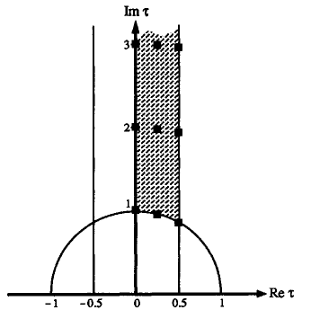
Figure 1: Fundamental domain of $\gamma(\tau)$.

Due to the quantization relation (4.2), the parameters $\tau$, $b$, and $n$ determine the lattice $\mathcal{L}$ up to a rotation and a translation. As the equations (2.1) are invariant under rotations and translations, solutions corresponding to translated and rotated lattices are related by symmetry transformations and therefore can be considered equivalent, with equivalence classes determined by triples $\omega=(\tau,b,n)$, specifying the underlying lattice has shape $\tau$, the average magnetic flux per lattice cell $b$, and the number $n$ of quanta of magnetic flux per lattice cell. With this in mind, we will say that an Abrikosov lattice state $(\Psi,A)$ is of type $\omega=(\tau,b,n)$, if it belong to the equivalence class determined by $\omega=(\tau,b,n)$.

Let $\beta(\tau)$ be the Abrikosov ’constant’, defined in (4.10) below. The following critical value of the Ginzburg-Landau parameter $\kappa$ plays an important role in what follows

$$\kappa_{c}(\tau):=\sqrt{\frac{1}{2}\left(1-\frac{1}{\beta(\tau)}\right)}.$$ (4.3)

Recall that the value of the second critical magnetic field at which the normal material undergoes the transition to the superconducting state is that $h_{c2}=\kappa^{2}$.

For the case $n=1$ of one quantum of flux per unit cell, the following result establishes the existence of non-trivial lattice solutions near the normal metal solution:

Theorem 4.1 ([58, 11, 28, 91]).

Fix a lattice shape $\lambda$ and let $b$ satisfy

$$|\kappa^{2}-b|\ll\kappa^{2}[(2\kappa^{2}-1)\beta(\tau)+1]$$ (4.4)

and

$$\text{either}\ \kappa>\kappa_{c}(\tau),\ \kappa^{2}>b\ \text{ or }\ \kappa<\kappa_{c}(\tau),\ \kappa^{2}<b.$$ (4.5)

Then for $\omega=(\tau,b,1)$

• there exists a smooth Abrikosov lattice solution $u_{\omega}=(\Psi_{\omega},A_{\omega})$ of type $\omega$.

Remark. For $\kappa>\frac{1}{\sqrt{2}}$ and the triangular and square lattices the theorem was proven in [58, 11, 28, 90] and in the case stated, in [90, 91].

Theorem 4.2 ([91]).

Let $\kappa>\frac{1}{\sqrt{2}}$. Fix a lattice shape $\tau$ and let $b$ satisfy $b<\kappa^{2}$ and (4.4). Then

• the global minimizer of the average energy per cell is the solution corresponding to the equilateral triangular lattice.

(Due to a calculation error, Abrikosov concluded that the lattice which gives the minimum energy is the square lattice. The error was corrected by Kleiner, Roth, and Autler [51], who showed that it is in fact the triangular lattice which minimizes the energy.)

Now, we formulate the existence result for low magnetic fields, those near the first critical magnetic field $h_{c1}$: Let $\mathcal{L}_{\omega}$ be a lattice specified by a triple $\omega=(\tau,b,n)$ and let $\Omega_{\omega}$ denote its elementary cell. We have

Theorem 4.3 ([76]).

Let $\kappa\neq\frac{1}{\sqrt{2}}$ and fix a lattice shape $\lambda$ and $n\neq 0$. Then there is $b_{0}=b_{0}(\kappa)\ (\sim(\kappa-1/\sqrt{2})^{2})>0$ such that for $b\leq b_{0}$, there exists an odd solution Abrikosov lattice solution $u_{\omega}\equiv(\Psi_{\omega},A_{\omega})$ of (2.1), s.t.

$$u_{\omega}(x)=u^{(n)}(x-\alpha)+O(e^{-c\rho})\ \text{ on }\ \Omega_{\omega}+\alpha,\ \forall\alpha\in\mathcal{L}_{\omega},$$ (4.6)

where $u^{(n)}:=(\Psi^{(n)},A^{(n)})$ is the $n-$vortex, $\rho=b^{-1/2}$ and $c>0$, in the sense of the local Sobolev norm of any index.

In the next two subsections we present a discussion of some key general notions. After this, we outline the proofs of the results above.

4.3 Abrikosov lattices as gauge-equivariant states

A key point in proving both theorems is to realize that a state $(\Psi,A)$ is an Abrikosov lattice if and only if $(\Psi,A)$ is gauge-periodic or gauge-equivariant (with respect to a lattice $\mathcal{L}$) in the sense that there exist (possibly multivalued) functions $g_{s}:\mathbb{R}^{2}\to\mathbb{R}$, $s\in\mathcal{L}$, such that

$$T^{\rm trans}_{s}(\Psi,A)=T^{\rm gauge}_{g_{s}}(\Psi,A).$$ (4.7)

Indeed, if state $(\Psi,A)$ satisfies (4.7), then all associated physical quantities are $\mathcal{L}-$periodic, i.e. $(\Psi,A)$ is an Abrikosov lattice. In the opposite direction, if $(\Psi,A)$ is an Abrikosov lattice, then $\operatorname{curl}A(x)$ is periodic w.r.to $\mathcal{L}$, and therefore $A(x+s)=A(x)+{\nabla}g_{s}(x)$, for some functions $g_{s}(x)$. Next, we write $\Psi(x)=|\Psi(x)|e^{i\phi(x)}$. Since $|\Psi(x)|$ and $J(x)=|\Psi(x)|^{2}({\nabla}\phi(x)-A(x))$ are periodic w.r.to $\mathcal{L}$, we have that ${\nabla}\phi(x+s)={\nabla}\phi(x)+{\nabla}\tilde{g}_{s}(x)$, which implies that $\phi(x+s)=\phi(x)+g_{s}(x)$, where $g_{s}(x)=\tilde{g}_{s}(x)+c_{s}$, for some constants $c_{s}$.

Since $T^{\rm trans}_{s}$ is a commutative group, we see that the family of functions $g_{s}$ has the important cocycle property

$$g_{s+t}(x)-g_{s}(x+t)-g_{t}(x)\in 2\pi\mathbb{Z}.$$ (4.8)

This can be seen by evaluating the effect of translation by $s+t$ in two different ways. We call $g_{s}(x)$ the gauge exponent. It can be shown (see Appendix B) that by a gauge transformation, we can pass from a exponential $g_{s}$ satisfying the cocycle condition (4.8) is equivalent to the exponent

$$\frac{b}{2}s\wedge x+c_{s},\ \text{ with $c_{s}$ satisfying }\ c_{s+t}-c_{s}-c_{t}-\frac{1}{2}bs\wedge t\in 2\pi\mathbb{Z},$$ (4.9)

for and $b$ satisfying $b|\Omega|\in 2\pi\mathbb{Z}$. For more discussion of $g_{s}$, see Appendix B.

Remark. Relation (4.8) for Abrikosov lattices was isolated in [77], where it played an important role. This condition is well known in algebraic geometry and number theory (see e.g. [38]). However, there the associated vector potential (connection on the corresponding principal bundle) $A$ is not considered there.

4.4 Abrikosov function

Let the number of the magnetic flux quant per the lattice cell be $n=1$. Let $\langle f\rangle_{\Omega}$ denote the average, $\langle f\rangle_{\Omega}=\frac{1}{|\Omega|}\int_{\Omega}f,$ of a function $f$ over $\Omega\subset\mathbb{R}^{2}$. For a lattice $\mathcal{L}$, considered as a group of lattice translations, $\hat{\mathcal{L}}$ denotes the dual group, i.e. the group of characters, $\chi:\mathcal{L}\to U(1)$. Furthermore, let $\mathcal{T}:=\mathbb{R}^{2}/\mathcal{L}$ and for $\mathcal{L}\in[\tau]$, we introduce the normalized lattice $\mathcal{L}_{\tau}=\sqrt{\frac{2\pi}{|\mathcal{T}|}}\mathcal{L}$. The key role in understanding the energetics of is played by the Abrikosov function,

$$\beta(\tau):=\frac{\langle|\phi|^{4}\rangle_{\Omega_{\tau}}}{\langle|\phi|^{2}\rangle_{\Omega_{\tau}}^{2}},$$ (4.10)

where $\Omega_{\tau}$ is a fundamental cell of the lattice $\mathcal{L}_{\tau}$, and $\phi$ is the solution to the problem

$$(-\Delta_{\!A^{n}}-n)\phi=0,\ \quad\phi(x+s)=e^{i\frac{n}{2}s\wedge x}\phi(x),\ \quad\forall s\in\mathcal{L}_{\tau},$$ (4.11)

where $A^{n}(x):=-\frac{n}{2}Jx$ and $J:=\left(\begin{array}[]{cc}0&1\\ -1&0\end{array}\right)$, for $n=1$. We will show below (Proposition 4.4) that, for $n=1$, the problem (4.11) has a unique solution and therefore $\beta$ is well-defined. It is not hard to see that $\beta$ depends only on the equivalence class of $\mathcal{L}$.

Definition (4.10) - (4.11) implies that $\beta(\tau)$ is symmetric w.r.to the imaginary axis, $\beta(-\bar{\tau})=\beta(\tau)$. Hence it suffices to consider $\beta(\tau)$ on the $\operatorname{Re}\tau\geq 0$ half of the fundamental domain, $\Pi^{+}/SL(2,\mathbb{Z})$ (the heavily shaded area on Fig. 1).

Moreover, we can consider (4.10) - (4.11) on the entire Poicaré half-plane $\Pi^{+}:=\{\tau\in\mathbb{C}:\operatorname{Im}\tau>0\}$, which allows us to define $\beta(\tau)$ as a modular function on $\Pi^{+}$,

• the function $\beta(\tau)$, defined on $\Pi^{+}$, is invariant under the action of $SL(2,\mathbb{Z})$.

This implies that it suffices to consider $\beta(\tau)$ on the fundamental domain (A.1).

Remarks. 1) The term Abrikosov constant comes from the physics literature, where one often considers only equilateral triangular or square lattices.

2) The way we defined the Abrikosov constant $\beta(\tau)$, it is manifestly independent of $b$. Our definition differs from the standard one by rescaling: the standard definition uses the function $\phi_{b}(x)=\phi(\sqrt{b}x)$, instead of $\phi(x)$.

4.5 Comments on the proof of Theorem 4.1

As was mentioned in Subsection 4.3, we look for solutions of (2.10), satisfying condition (4.7), or explicitly as, for $s\in\mathcal{L}$,

$$\begin{cases}\Psi(x+s)=e^{ig_{s}(x)}\Psi(x),\\ A(x+s)=A(x)+{\nabla}g_{s}(x),\end{cases}$$ (4.12)

where $g_{s}$ satisfies (4.8). By (4.9), it can be taken to be

$$g_{s}(x)=\frac{b}{2}s\wedge x+c_{s},$$ (4.13)

where $b$ is the average magnetic flux, $b=\frac{1}{|\Omega|}\int_{\Omega}\operatorname{curl}A$ (satisfying (4.2) so that $bs\wedge t\in 2\pi\mathbb{Z}$), and the $c_{s}$ satisfy

$$c_{s+t}-c_{s}-c_{t}-\frac{1}{2}bs\wedge t\in 2\pi\mathbb{Z}.$$ (4.14)

The linearized problem.

We expect that as the average flux $b$ decreases below $h_{c2}=\kappa^{2}$, a vortex lattice solution emerges from the normal material solution $(\Psi_{n},A_{n})$, where $\Psi_{n}=0$ and $A_{n}$ is a magnetic potential, with the constant magnetic field $b$. Note that $(\Psi_{n},A_{n})=(0,A^{b})$ satisfies (4.12), if we take the gauge $A^{b}=-\frac{b}{2}Jx$. Linearizing (2.1) at $(0,A^{b})$, leads to the linearized problem

$$(-\Delta_{\!A^{b}}-\kappa^{2})\phi=0,$$ (4.15)

with $\phi(x)$ satisfying

$$\phi(x+s)=e^{i\frac{b}{2}s\cdot Jx}\phi(x),\ \quad\forall s\in\mathcal{L}.$$ (4.16)

(The second equation in (2.1) leads to $\operatorname{curl}a=0$ which gives, modulo gauge transformation, $a=0$.) We show that this problem has $n$ linearly independent solutions, provided $b|\Omega|=2\pi n$ and $b=\kappa^{2}=h_{c2}$.

Denote by $L^{b}$ the operator $-\Delta_{A^{b}}$, defined on the lattice cell $\Omega$ with the lattice boundary conditions in (4.16), is self-adjoint, has a purely discrete spectrum, and evidently satisfies $L^{b}\geq 0$. We have

Proposition 4.4.

The operator $L^{b}$ is self-adjoint, with the purely discrete spectrum given by the spectrum explicitly as

$$\sigma(L^{b})=\{\,(2k+1)b:k=0,1,2,\ldots\,\},$$ (4.17)

and each eigenvalue is of the same multiplicity.

If $b|\Omega|=2\pi n$, then this multiplicity is $n$ and, in particular, we have

$$\dim_{\mathbb{C}}\operatorname{Null}(L^{b}-b)=n.$$

Proof.

The self-adjointness is standard. Spectral information about $L^{b}$ can be obtained by introducing the harmonic oscillator annihilation and creation operators, $\alpha$ and $\alpha^{*}$, with

$$\alpha:=(\nabla_{A^{b}})_{1}+i(\nabla_{A^{b}})_{2}=\partial_{x_{1}}+i\partial_{x_{2}}+\frac{1}{2}bx_{1}+\frac{1}{2}ibx_{2}.$$ (4.18)

One can verify that these operators satisfy the following relations:

1. $[\alpha,\alpha^{*}]=2\operatorname{curl}A^{b}=2b$;

2. $-\Delta_{A^{b}}-b=\alpha^{*}\alpha$.

As for the harmonic oscillator (see for example [41]), this gives the spectrum explicitly, (4.17). This proves the first part of the theorem.

For the second part, a simple calculation gives the following operator equation

$$e^{\frac{b}{2}(ix_{1}x_{2}-x_{2}^{2})}\alpha e^{-\frac{b}{2}(ix_{1}x_{2}-x_{2}^{2})}=\partial_{x_{1}}+i\partial_{x_{2}}.$$

This immediately proves that $\psi\in\operatorname{Null}\alpha$ if and only if $\xi(x)=e^{\frac{b}{2}(ix_{1}x_{2}-x_{2}^{2})}\psi(x)$ satisfies $\partial_{x_{1}}\xi+i\partial_{x_{2}}\xi=0$.

We identify $\mathbb{R}^{2}$ with $\mathbb{C}$, via the map $(x_{1},x_{2})\rightarrow x_{1}+ix_{2}$. We can choose a basis in $\mathcal{L}$ so that $\mathcal{L}=r(\mathbb{Z}+\tau\mathbb{Z})$, where $\tau\in\mathbb{C}$, $\operatorname{Im}\tau>0$, and $r>0$. By the quantization condition (4.2), $r:=\sqrt{\frac{2\pi n}{\operatorname{Im}\tau b}}$. Define $z=\frac{1}{r}(x_{1}+ix_{2})$ and

$$\theta(z)=e^{\frac{b}{2}(ix_{1}x_{2}-x_{2}^{2})}\phi(x).$$ (4.19)

By the above, the function $\theta$ is entire and, due to the periodicity conditions on $\phi$, satisfies

$$\theta(z+1)=\theta(z),$$ (4.20)

$$\theta(z+\tau)=e^{-2inz}e^{-in\tau z}\theta(z).$$

Hence $\theta$ is the theta function and has the absolutely convergent Fourier expansion

$$\theta(z)=\sum_{k=-\infty}^{\infty}c_{k}e^{2kiz}.$$ (4.21)

with the coefficients satisfying $c_{k+n}=e^{in\pi\tau}e^{2ki\pi\tau}c_{k},$ which means such functions are determined by $c_{0},\ldots,c_{n-1}$ and therefore form an $n$-dimensional vector space. This proves Proposition 4.4. ∎

This also gives the form of the leading approximation (4.19) - (4.21) to the true solution.

The nonlinear problem.

Now let $n=1$. Once the linearized map is well understood, it is possible to construct solutions, $u_{\omega},\ \omega=(\tau,b,1)$, of the Ginzburg-Landau equations for a given lattice shape parameter $\tau$, and the average magnetic flux $b$ near $h_{c2}$, via a Lyapunov-Schmidt reduction.

4.6 Comments on the proof of Theorem 4.2

The relation between the Abrikosov function and the average energy, $E_{b}(\tau):=\frac{1}{|\Omega^{\tau}|}{\cal E}_{\Omega^{\tau}}(u_{\omega})$, of this solution is given by

Proposition 4.5.

In the case $\kappa>\frac{1}{\sqrt{2}}$, the minimizers, $\tau_{b}$, of $\tau\mapsto E_{b}(\tau)$ are related to the minimizer, $\tau_{*}$, of $\beta(\tau)$, as $\tau_{b}-\tau_{*}=O(\mu^{1/2})$, In particular, $\tau_{b}\to\tau_{*}$ as $b\to\kappa^{2}$.

This result was already found (non-rigorously) by Abrikosov [1]. Thus the problem of minimization of the energy per the lattice cell is reduced to finding the minima of $\beta(\tau)$ as a function of the lattice shape parameter $\tau$.

Using symmetries of $\beta(\tau)$ one can also show (see [78] and below) that $\beta(\tau)$ has critical points at the points $\tau=e^{\pi i/3}$ and $\tau=e^{\pi i/2}$. However, to determine minimizers of $\beta(\tau)$ requires a rather delicate analysis, which gives

Theorem 4.6 ([2, 57]).

The function $\beta(\tau)$ has exactly two critical points, $\tau=e^{i\pi/3}$ and $\tau=e^{i\pi/2}$. The first is minimum, while the second is a maximum.

Hence the second part of Theorem 4.2 follows.

4.7 Comments on the proof of Theorem 4.3

The idea here is to reduce solving (2.1) for $(\Psi,A)$ on the space $\mathbb{R}^{2}$ to solving it for $(\psi,a)$ on the fundamental cell $\Omega$, satisfying the boundary conditions

$$\begin{cases}\psi(x+s)=e^{ig_{s}(x)}\psi(x),\\ a(x+s)=a(x)+\nabla g_{s}(x),\\ (\nu\cdot\nabla_{a}\psi)(x+s)=e^{ig_{s}(x)}(\nu\cdot\nabla_{a}\psi)(x),\\ \operatorname{curl}a(x+s)=\operatorname{curl}a(x),\\ x\in\partial_{1}\Omega/\partial_{2}\Omega\ \mbox{and}\ s=\omega_{1}/\omega_{2}.\end{cases}$$ (4.22)

induced by the periodicity condition (4.12). Here $\partial_{1}\Omega/\partial_{2}\Omega=$ the left/bottom boundary of $\Omega$, $\{\omega_{1},\omega_{2}\}$ is a basis in $\mathcal{L}$ and $\nu(x)$ is the normal to the boundary at $x$.

To this end we show that, given a continuously differentiable function $(\psi,a)$ on the fundamental cell $\Omega$, satisfying the boundary conditions (4.22), with $g_{s}$ satisfying (4.8), we can lift it to a continuous and continuously differentiable function $(\Psi,A)$ on the space $\mathbb{R}^{2}$, satisfying the gauge-periodicity conditions (4.12). Indeed, we define for any $\alpha\in\mathcal{L}$,

$$\Psi(x)=\psi(x-\alpha)e^{i\Phi_{\alpha}(x)},\ A(x)=a(x-\alpha)+\nabla\Phi_{\alpha}(x),\ x\in\Omega+\alpha,$$ (4.23)

where $\Phi_{\alpha}(x)$ is a real, possibly multi-valued, function to be determined. (Of course, we can add to it any $\mathcal{L}-$periodic function.) We define

$$\Phi_{\alpha}(x):=g_{\alpha}(x-\alpha),\ \mbox{for}\ x\in\Omega+\alpha.$$ (4.24)

Lemma 4.7.

Assume functions $(\psi,a)$ on $\Omega$ are twice differentiable, up to the boundary, and obey the boundary conditions (4.22) and the Ginzburg-Landau equations (2.1). Then the functions $(\Psi,A)$, constructed in (4.23) - (4.24), are smooth in $\mathbb{R}^{2}$ and satisfy the periodicity conditions (4.12) and the Ginzburg-Landau equations (2.1).

Proof.

If $(\psi,a)$ satisfies the Ginzburg-Landau equations (2.1) in $\Omega$, then $U\equiv(\Psi,A)$, constructed in (4.23) - (4.24), has the following properties

• $(\Psi,A)$ is twice differentiable and satisfies (2.1) in $\mathbb{R}^{2}/(\cup_{t\in\mathcal{L}}S_{t}\partial\Omega)$, where $S_{t}:x\rightarrow x+t$;

• $(\Psi,A)$ is continuous with continuous derivatives ($\nabla_{A}\Psi$ and $\operatorname{curl}A$) in $\mathbb{R}^{2}$ and satisfies the gauge-periodicity conditions (4.12) in $\mathbb{R}^{2}$.

Indeed, the periodicity condition (4.12), applied to the cells $\Omega+\alpha-\omega_{i}$ and $\Omega+\alpha$ and the continuity condition on the common boundary of the cells $\Omega+\alpha-\omega_{i}$ and $\Omega+\alpha$ imply that $\Phi_{\alpha}(x)$ should satisfy the following two conditions:

$$\Phi_{\alpha}(x)=\Phi_{\alpha-\omega_{i}}(x-\omega_{i})+g_{\omega_{i}}(x-\omega_{i}),\ \mbox{mod}\ 2\pi,\ x\in\Omega+\alpha,$$ (4.25)

$$\Phi_{\alpha}(x)=\Phi_{\alpha-\omega_{i}}(x)+g_{\omega_{i}}(x-\alpha),\ \mbox{mod}\ 2\pi,\ x\in\partial_{i}\Omega+\alpha,$$ (4.26)

where $i=1,2,$ and, recall, $\{\omega_{1},\omega_{2}\}$ is a basis in $\mathcal{L}$ and $\partial_{1}\Omega/\partial_{2}\Omega$ is the left/bottom boundary of $\Omega$.

To show that (4.24) satisfies the conditions (4.25) and (4.26), we note that, due to (4.8), we have $g_{\alpha}(x-\alpha)=g_{\alpha-\omega_{i}}(x-\alpha)+g_{\omega_{i}}(x-\omega_{i}),\ \mbox{mod}\ 2\pi,\ x\in\Omega+\alpha,$ and $g_{\alpha}(x-\alpha)=g_{\alpha-\omega_{i}}(x-\alpha+\omega_{i})+g_{\omega_{i}}(x-\alpha),\ \mbox{mod}\ 2\pi,\ x\in\partial_{i}\Omega+\alpha$, which are equivalent to (4.25) and (4.26), with (4.24).

The second pair of conditions in (4.22) implies that $\nabla_{A}\Psi$ and $\operatorname{curl}A$ are continuous across the cell boundaries.

By (a) and (b), the derivatives $\Delta_{A}\Psi$ and $\operatorname{curl}^{2}A$ are continuous, up to the boundary, in $S_{t}\partial\Omega,$ for every $t\in\mathcal{L}$. By (2.1), they are equal in $\mathbb{R}^{2}/(\cup_{t\in\mathcal{L}}S_{t}\partial\Omega)$ to functions continuous in $\mathbb{R}^{2}$ satisfying there the periodicity condition (4.12). Hence, they are also continuous and satisfy the periodicity condition (4.12) in $\mathbb{R}^{2}$. By iteration of the above argument (i.e. elliptic regularity), $\Psi,A$ are smooth functions obeying (4.12) and (2.1). ∎

Now, we use the $n-$vortex $(\Psi^{(n)},A^{(n)})$, placed in the centre of the fundamental cell $\Omega$, to construct an approximate solution $(\psi^{\rm appr},a^{\rm appr})$ to (2.1) in $\Omega$, satisfying (4.22), and use it and the Lyapunov-Schmidt splitting technique to show that there is a true solution $(\psi,a)$ nearby sharing the same properties. After that, we use Lemma 4.7 above to lift $(\psi,a)$ to a solution $(\Psi,A)$ on the space $\mathbb{R}^{2}$, satisfying the gauge-periodicity conditions (4.12).

4.8 Stability of Abrikosov lattices

The Abrikosov lattices are static solutions to (2.10) and their stability w.r. to the dynamics induced by these equations is an important issue. In [77], we considered the stability of the Abrikosov lattices for magnetic fields close to the second critical magnetic field $h_{c2}=\kappa^{2}$, under the simplest perturbations, namely those having the same (gauge-) periodicity as the underlying Abrikosov lattices (we call such perturbations gauge-periodic) and proved for a lattice of arbitrary shape, $\tau\in\mathbb{C}$, $\operatorname{Im}\tau>0$, that, under gauge-periodic perturbations, Abrikosov vortex lattice solutions are

• asymptotically stable for $\kappa^{2}>\kappa_{c}(\tau)$;

• unstable for $\kappa^{2}<\kappa_{c}(\tau)$.

This result belies the common belief among physicists and mathematicians that Abrikosov-type vortex lattice solutions are stable only for triangular lattices and $\kappa>\frac{1}{\sqrt{2}}$, and it seems this is the first time the threshold (4.3) has been isolated.

In [76], similar results are shown to hold also for low magnetic fields close to $h_{c1}$.

Gauge-periodic perturbations are not a common type of perturbations occurring in superconductivity. Now, we address the problem of the stability of Abrikosov lattices under local or finite-energy perturbations (defined precisely below). We consider Abrikosov lattices of arbitrary shape, not just triangular or rectangular lattices as usually considered, and for magnetic fields close to the second critical magnetic field $h_{c2}=\kappa^{2}$.

Finite-energy ($H^{1}-$) perturbations.

We now wish to study the stability of these Abrikosov lattice solutions under a class of perturbations that have finite-energy. More precisely, we fix an Abrikosov lattice solution $u_{\omega}$ and consider perturbations $v:\mathbb{R}^{2}\to\mathbb{C}\times\mathbb{R}^{2}$ that satisfy

$$\Lambda_{u_{\omega}}(v)=\lim_{Q\rightarrow\mathbb{R}^{2}}\big{(}{\cal E}_{Q}(u_{\omega}+v)-{\cal E}_{Q}(u_{\omega})\big{)}<\infty.$$ (4.27)

Clearly, $\Lambda_{u_{\omega}}(v)<\infty$ for all vectors of the form $v=T^{\rm gauge}_{\gamma}u_{\omega}-u_{\omega}$, where $\gamma\in H^{2}(\mathbb{R}^{2};\mathbb{R})$.

In fact, we will be dealing with the smaller class, $H^{1}_{\textrm{cov}}$, of perturbations, where $H^{1}_{\textrm{cov}}$ is the Sobolev space of order $1$ defined by the covariant derivatives, i.e.,

$$H^{1}_{\textrm{cov}}:=\{v\in L^{2}(\mathbb{R}^{2},\mathbb{C}\times\mathbb{R}^{2})\ |\ \|v\|_{H^{1}}<\infty\},$$

where the norm $\|v\|_{H^{1}}$ is determined by the covariant inner product

$$\langle v,v^{\prime}\rangle_{H^{1}}=\operatorname{Re}\int\bar{\xi}\xi^{\prime}+\overline{\nabla_{\!\!A_{\omega}}\xi}\cdot\nabla_{\!\!A_{\omega}}\xi^{\prime}+\alpha\cdot\alpha^{\prime}+\sum_{k=1}^{2}\nabla\alpha_{k}\cdot\nabla\alpha^{\prime}_{k},$$

where $v=(\xi,\alpha),\ v^{\prime}=(\xi^{\prime},\alpha^{\prime})$, while the $L^{2}-$norm is given by

$$\langle v,v^{\prime}\rangle_{L^{2}}=\operatorname{Re}\int\bar{\xi}\xi^{\prime}+\alpha\cdot\alpha^{\prime}.$$ (4.28)

An explicit representation for the functional $\Lambda_{u_{\omega}}(v)$, given below shows (see (4.40)) that $\Lambda_{u_{\omega}}(v)<\infty$ for all vectors $v\in H^{1}_{\textrm{cov}}$.

To introduce the notions of stability and instability, we note that the hessian Hess ${\cal E}(u)$ is well defined as a differential operator for say $u\in u_{\omega}+H^{1}_{\textrm{cov}}$ and is a real-linear operator on $H^{1}_{\textrm{cov}}$. We define the manifold

$$\mathcal{M}_{\omega}=\{T^{\rm gauge}_{\gamma}u_{\omega}:\gamma\in H^{1}(\mathbb{R}^{2},\mathbb{R})\}$$

of gauge equivalent Abrikosov lattices and the $H^{1}-$distance, $\operatorname{dist}_{H^{1}}$, to this manifold.

Definition 4.8.

We say that the Abrikosov lattice $u_{\omega}$ is asymptotically stable under $H^{1}_{\textrm{cov}}-$ perturbations, if there is $\delta>0$ s.t. for any initial condition $u_{0}$ satisfying $\operatorname{dist}_{H^{1}}(u_{0},\mathcal{M}_{\omega})\leq\delta$ there exists $g(t)\in H^{1}$, s.t. the solution $u(t)$ of (2.10) satisfies $\|u(t)-T^{\rm gauge}_{g(t)}u_{\omega}\|_{H^{1}}\rightarrow 0$, as $t\rightarrow\infty$. We say that $u_{\omega}$ is energetically unstable if the hessian, ${\cal E}^{\prime\prime}(u_{\omega})$, of ${\cal E}(u)$ at $u_{\omega}$ has a negative spectrum.

We restrict the initial conditions $(\Psi_{0},A_{0})$ for (2.10) satisfying

$$T^{\rm refl}(\Psi_{0},A_{0})=(\Psi_{0},A_{0}).$$ (4.29)

Note that, by uniqueness, the Abrikosov lattice solutions $u_{\omega}=(\Psi_{\omega},A_{\omega})$ satisfy $T^{\rm refl}u_{\omega}=u_{\omega}$ and therefore so are the perturbations, $v_{0}:=u_{0}-u_{\omega}$, where $u_{0}:=(\Psi_{0},A_{0})$:

$$T^{\rm refl}v_{0}=v_{0}.$$ (4.30)

Stability result.

Recall that $\beta(\tau)$ is the Abrikosov ’constant’, introduced in (4.10).

Theorem 4.9.

There exists a modular function $\gamma(\tau)$ depending on the lattice shape parameters $\tau$, such that, for $b$ sufficiently close to $\kappa^{2}$, in the sense of (4.4), and, under $H^{1}-$perturbations, satisfying (4.29),

• the Abrikosov lattice $u_{\omega}$ is asymptotically stable for all $(\tau,\kappa)$ s.t. $\kappa>\frac{1}{\sqrt{2}}$ and $\gamma(\tau)>0$ and

• energetically unstable otherwise.

The function $\gamma(\tau),\ \operatorname{Im}\tau>0,$ appearing in the theorem above is described below. Meantime we make the following important remark. Since we know that, for $\kappa>1/\sqrt{2}$, the triangular lattice has the lowest energy (see Theorem 4.1), this seems to suggest that other lattices should be unstable. The reason that this energetics does not affect the stability under local perturbations can be gleaned from investigating the zero mode of the Hessian of the energy functional associated with different lattice shapes, $\tau$. This mode is obtained by differentiating the Abrikosov lattice solutions w.r.to $\tau$, which shows that it grows linearly in $|x|$. To rearrange a non - triangular Abrikosov lattice into the triangular one, one would have to activate this mode and hence to apply a perturbation, growing at infinity (at the same rate).

This also explains why the Abrikosov ’constant’ $\beta(\tau)$ mentioned above, which plays a crucial role in understanding the energetics of the Abrikosov solutions, is not directly related to the stability under local perturbations, the latter is governed by $\gamma(\tau)$.

4.9 The function $\gamma(\tau)$

Theorem 4.10.

The function $\gamma(\tau)$ on lattice shapes $\tau$, entering Theorem 4.9, is given by

$$\gamma(\tau):=\inf_{\chi\in\hat{\mathcal{L}}_{\tau}}\gamma_{\chi}(\tau),\ \text{ where }\ \gamma_{\chi}(\tau):=2\langle|\phi_{0}|^{2}|\phi_{\chi}|^{2}\rangle_{\mathcal{T}_{\tau}}+|\langle\phi_{0}^{2}\bar{\phi}_{\chi}\bar{\phi}_{\chi^{-1}}\rangle_{\mathcal{T}_{\tau}}|-\langle|\phi_{0}|^{4}\rangle_{\mathcal{T}_{\tau}}.$$ (4.31)

Here the functions $\phi_{\chi},\ \chi\in\hat{\mathcal{L}}_{\tau},$ are unique solutions of the equations

$$(-\Delta_{\!A^{1}}-1)\phi=0,\ \quad\phi(x+s)=e^{i\frac{1}{2}s\cdot Jx}\chi(s)\phi(x),\ \quad\forall s\in\mathcal{L}_{\tau},$$ (4.32)

with $A^{1}(x):=-\frac{1}{2}Jx$ and $J:=\left(\begin{array}[]{cc}0&1\\ -1&0\end{array}\right)$, normalized as $\langle|\phi_{\chi}|^{2}\rangle_{\mathcal{T}_{\tau}}=1$.

For the function $\gamma(\tau),\ \operatorname{Im}\tau>0,$ defined in (4.31), has the following properties

• $\gamma(\tau),\ \operatorname{Im}\tau>0,$ is symmetric w.r.to the imaginary axis, $\gamma(-\bar{\tau})=\gamma(\tau);$

• $\gamma(\tau)$ has critical points at $\tau=e^{i\pi/2}$ and $\tau=e^{i\pi/3}$, provided it is differentiable at these points.

We see also that the the Abrikosov constant, $\beta(\tau)$, is related to $\gamma_{k}(\tau)$ as $\beta(\tau)=\frac{1}{2}\gamma_{0}(\tau)$.

The function $\gamma(\tau)$ is studied numerically in [78], where the above conjecture is confirmed and is shown that it becomes negative for $\operatorname{Im}\tau\geq 1.81$. Moreover, it is computed that

$$|\gamma(\tau)-c| \leq 7.5\cdot 10^{-3},\ \ \quad\mbox{where}\$$

$$c=0.64\ \mbox{for}\ \tau=e^{i\pi/3}\quad\mbox{and}\ \quad c=0.4\ \mbox{for}\ \tau=e^{i\pi/2}.$$ (4.33)

The definition of $\gamma(\tau)$ implies that it is symmetric w.r.to the imaginary axis, $\gamma(-\bar{\tau})=\gamma(\tau)$. Hence it suffices to consider $\gamma(\tau)$ on the $\operatorname{Re}\tau\geq 0$ half of the fundamental domain, $\Pi^{+}/SL(2,\mathbb{Z})$, of the modular group $SL(2,\mathbb{Z})$ (the heavily shaded area on the Fig. 1 above). Using the symmetries of $\gamma(\tau)$, we show in [78] that the points $\tau=e^{i\pi/2}$ and $\tau=e^{i\pi/3}$ are critical points of the function $\gamma(\tau)$, provided it is differentiable at these points. (While the functions $\gamma_{k}(\tau)$ are obviously smooth, derivatives of $\gamma(\tau)$ might jump. In fact, the numerical computations described in [78] show that $\gamma(\tau)$ is likely to have the line of cusps at $\operatorname{Re}\tau=0$.) We conjecture:

• For fixed $\operatorname{Re}\tau\in[0,1/2]$, $\gamma(\tau)$ is a decreasing function of $\operatorname{Im}\tau$.

• $\gamma(\tau)$ has a unique global maximum at $\tau=e^{\frac{i\pi}{3}}$ and a saddle point at $\tau=e^{\frac{i\pi}{2}}$.

In [78], we confirm this conjecture numerically (numerics is due to Dan Ginsberg, see Figure 2 for the result of computing $\gamma(\tau)$ in Matlab, using the default Nelder-Mead algorithm).

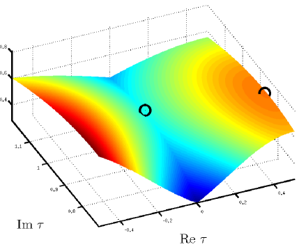
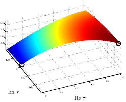
Figure 2: Plots of the function $\gamma^{approx}(\tau)$. Computed in Matlab on a uniform grid with step size 0.01. The plot on the right is the function plotted only on the Poincaré strip. The circled points are $\tau=e^{i\pi/2}$ and $\tau=e^{i\pi/3}$.

Calculations of [78] show that $\gamma(\tau)>0$ for all equilateral lattices, $|\tau|=1$, and is negative for $|\tau|\geq 1.3$. Though Abrikosov lattices are not as rigid under finite energy perturbations, as for gauge-periodic ones, they are still surprisingly stable.

It is convenient to consider $\gamma(\tau)$ as a modular function on $\Pi^{+}$. To this end, recalling that we identify $\mathbb{R}^{2}$ with $\mathbb{C}$, via the map $(x_{1},x_{2})\rightarrow x_{1}+ix_{2}$, we can choose a basis in $\mathcal{L}$ so that $\mathcal{L}=r(\mathbb{Z}+\tau\mathbb{Z})$, where $\tau\in\mathbb{C}$, $\operatorname{Im}\tau>0$, and $r>0$. By the quantization condition (4.2) with $n=1$, $r:=\sqrt{\frac{2\pi}{\operatorname{Im}\tau b}}$. Denote $\mathcal{L}_{\tau}=\sqrt{\frac{2\pi}{\operatorname{Im}\tau}}(\mathbb{Z}+\tau\mathbb{Z})$. The dual to it is $\mathcal{L}^{*}_{\tau}=\sqrt{\frac{2\pi}{\operatorname{Im}\tau}}i(\mathbb{Z}-\tau\mathbb{Z})$. (The dual, or reciprocal, lattice, $\mathcal{L}^{*}$, of $\mathcal{L}$ consists of all vectors $s^{*}\in\mathbb{R}^{2}$ such that $s^{*}\cdot s\in 2\pi\mathbb{Z}$, for all $s\in\mathcal{L}$.) We identify the dual group, $\hat{\mathcal{L}}_{\tau}$, with a fundamental cell, $\Omega^{*}_{\tau}$, of the dual lattice $\mathcal{L}^{*}_{\tau}$, chosen so that $\Omega^{*}_{\tau}$ is invariant under reflections, $k\rightarrow-k$. This identification given explicitly by $\chi(s)\rightarrow\chi_{k}(s)=e^{ik\cdot s}\leftrightarrow k$.

Then the functions $\gamma(\tau)$ and $\gamma_{k}(\tau)=\gamma_{\chi_{k}}(\tau),\ \chi_{k}(s)=e^{ik\cdot s},\ k\in\Omega^{*}_{\tau}$, are defined in (4.31) for all $\tau,\operatorname{Im}\tau>0$. Since they are independent of the choice of a basis in $\mathcal{L}_{\tau}$, they are invariant under action of the modular group $SL(2,\mathbb{Z})$, $\gamma(g\tau)=\gamma(\tau),\ \forall g\in SL(2,\mathbb{Z})$, i.e. they modular functions on $\Pi^{+}$.

The numerics mentioned above are based on the following explicit representation of the functions $\gamma_{k}(\tau)$:

Theorem 4.11.

The functions $\gamma_{k}(\tau)$ admit the explicit representation

$$\gamma_{k}(\tau) =2\sum_{t\in\mathcal{L}_{\tau}^{*}}e^{-\frac{1}{2}|t|^{2}}\cos[\operatorname{Im}(\bar{k}t)]+|\sum_{t\in\mathcal{L}_{\tau}^{*}}e^{-\frac{1}{2}|t+k|^{2}+i\operatorname{Im}(\bar{k}t)}|-\sum_{t\in\mathcal{L}_{\tau}^{*}}e^{-\frac{1}{2}|t|^{2}}.$$ (4.34)

Our computations show also that

• $\gamma_{k}(\tau)$ is minimized at $k\approx\sqrt{\frac{2\pi}{\operatorname{Im}\tau b}}(\frac{1}{2}-\frac{1}{2\sqrt{3}}i)$ at the point $\tau=e^{i\pi/3}$, and a value of $k\approx\sqrt{\frac{2\pi}{\operatorname{Im}\tau b}}(\frac{1}{2}+i\frac{1}{2})$ for $\tau=e^{i\pi/2}$, which corresponds to vertices of the corresponding Wigner-Seitz cells.

Interestingly, in [78], we show that the points $k\in\frac{1}{2}\mathcal{L}^{*}_{\tau}$ are critical points of the function $\gamma_{k}(\tau)$ in $k$. It is easy to see that $k=0$ is a point of maximum of $\gamma_{k}(\tau)$ in $k\in\Omega^{*}_{\tau}$.

Remark. We think of $\gamma_{k}(\tau)$ as the ’Abrikosov beta function with characteristic’ (while $\beta(\tau)$ is defined in terms of the standard theta function, $\gamma_{k}(\tau)$ is defined in terms of theta functions with finite characteristics, see below).

4.10 The key ideas of approach

Let $u_{\omega}=(\Psi_{\omega},A_{\omega}),\ \omega:=(\tau,b,1),$ be an Abrikosov lattice solution. As usual, one begins with the Hessian $L_{\omega}:={\cal E}^{\prime\prime}(u_{\omega})$ of the energy functional ${\cal E}$ at $u_{\omega}$. To begin with, due to the fact that the solution $u_{\omega}$ of (2.1) breaks the gauge invariance, the operator $L_{\omega}$ has the gauge zero modes, $L_{\omega}G_{\gamma^{\prime}}=0$, where $G_{\gamma^{\prime}}:=(i\gamma^{\prime}\Psi_{\omega},\nabla\gamma^{\prime})$. Then the stability of the static solution $u_{\omega}$ is decided by the sign of the infimum $\mu(\omega,\kappa):=\inf_{v\in H^{1}_{\perp}}\langle v,L_{\omega}v\rangle_{L^{2}}/\|v\|_{L^{2}}^{2}$, on the subspace $H^{1}_{\perp}$ of the Sobolev space $H^{1}_{\textrm{cov}}$, which is the orthogonal complement of the these zero modes $G_{\gamma^{\prime}}$.

The key idea of the proof of the first part of Theorem 4.9 stems from the observation that since the Abrikosov lattice solution $u_{\omega}=(\Psi_{\omega},A_{\omega})$ is gauge periodic (or equivariant) w.r.to the lattice $\mathcal{L}_{\omega}$, i.e. satisfies (4.7) - (4.8), the linearized map $L_{\omega}$ commutes with magnetic translations,

$$\rho_{s}=T_{s}^{\rm mag-trans}\oplus T^{\rm trans}_{s},\ \quad\forall s\in\mathcal{L}_{\omega},$$ (4.35)

where $T_{s}^{\rm mag-trans}=(T^{gauge}_{g_{s}})^{-1}T^{\rm trans}_{s}$ is the group of magnetic translations and, recall, $T^{\rm trans}_{s}$ denotes translation by $s$, which, due to (4.8), give a unitary group representation of $\mathcal{L}_{\omega}$. (Note that (4.7) implies that $u_{\omega}$ is invariant under the magnetic translations, $T_{s}^{\rm mag-trans}u_{\omega}=u_{\omega}$.) Therefore $L_{\omega}$ is unitary equivalent to a fiber integral over the dual group, $\hat{\mathcal{L}}_{\omega}$, of the group of lattice translations,

$$L_{\omega}\approx\int_{\hat{\mathcal{L}}_{\omega}}^{\oplus}L_{\omega\chi}\hat{d\chi}\ \quad\mbox{acting on}\ \quad\int_{\hat{\mathcal{L}}_{\omega}}^{\oplus}\mathcal{H}_{\chi}\hat{d\chi}.$$ (4.36)

Here $\hat{d\chi}$ is the usual Lebesgue measure normalized so that $\int_{\hat{\mathcal{L}}_{\omega}}\hat{d\chi}=1$, $L_{\omega\chi}$ is the restriction of $L_{\omega}$ to $\mathcal{H}_{\chi}$ and $\mathcal{H}_{\chi}$ is the set of all functions, $v_{k}$, from $L^{2}_{\rm loc}(\mathbb{R}^{2};\mathbb{C}\times\mathbb{R}^{2})$, satisfying the gauge-periodicity conditions

$$\rho_{s}v_{\chi}(x)=\chi(s)v_{\chi}(x),\ \forall s\in\ \mathcal{L}_{\omega},$$ (4.37)

where $\chi:\mathcal{L}_{\omega}\to U(1)$ are the characters acting on $v=(\xi,\alpha)$ as the multiplication operators

$$\chi(s)v=(\chi(s)\xi,\chi(s)\alpha).$$

Furthermore, $\mathcal{H}_{\chi}$ is endowed with the inner product $\langle v,v^{\prime}\rangle_{L^{2}}=\frac{1}{|\mathcal{T}_{\omega}|}\int_{\mathcal{T}_{\omega}}\operatorname{Re}\bar{\xi}\xi^{\prime}+\bar{\alpha}\alpha^{\prime},$ where $\mathcal{T}_{\omega}:=\mathbb{R}^{2}/\mathcal{L}_{\omega}$ is a $2-$torus and $v=(\xi,\alpha),\ v^{\prime}=(\xi^{\prime},\alpha^{\prime})$. The inner product in $\int_{\hat{\mathcal{L}}_{\omega}}^{\oplus}\mathcal{H}_{\chi}\hat{d\chi}$ is given by $\langle v,w\rangle_{\mathcal{H}}:=\frac{1}{|\hat{\mathcal{L}}_{\omega}|}\int_{\hat{\mathcal{L}}_{\omega}}\langle v_{\chi},w_{\chi}\rangle_{\mathcal{H}_{\chi}}\hat{d\chi}$.

The decomposition (4.36) implies that the smallest spectral point, $\mu_{\omega}(\kappa)$, of $L_{\omega}$ is given by $\mu_{\omega}(\kappa)=\inf_{k\in\Omega^{*}_{\omega}}\mu_{\omega,\chi}(\kappa)$, where $\mu_{\omega,\chi}(\kappa)$ are the smallest eigenvalues of $L_{\omega\chi}$. The spectral analysis of fibers $L_{\omega\chi},\ \chi\in\hat{\mathcal{L}}_{\omega}^{*},$ using a natural perturbation parameter $\epsilon$ defined as

$$\epsilon=\sqrt{\frac{\kappa^{2}-b}{\kappa^{2}[(2\kappa^{2}-1)\beta(\tau)+1]}},$$ (4.38)

gives leads to the following expression for $\mu_{\omega,k}(\kappa)$ The lowest eigenvalue, $\mu_{\omega,\chi}(\kappa)$, of the operator $L_{\chi}$ on the subspace $\mathcal{H}_{\chi\perp}$ of $\mathcal{H}_{\chi}$, which is the orthogonal complement of the the $\chi-$fibers of the gauge zero modes $G_{\gamma^{\prime}}:=(i\gamma^{\prime}\Psi_{\omega},\nabla\gamma^{\prime})$, are of the form

$$\mu_{\omega,\chi}(\kappa)=(\kappa^{2}-\frac{1}{2})\gamma_{\chi}(\tau)\epsilon^{2}+O(\epsilon^{3}),$$ (4.39)

for $\chi\neq 1$, with the functions $\gamma_{\chi}(\tau)$ defined in (4.31) and (4.32).

The linear result above gives the linearized (energetic) stability of $u_{\omega}$, if $\mu_{\omega,\chi}(\kappa)>0$, and the instability, if $\mu_{\omega,\chi}(\kappa)<0$. To lift the stability part to the (nonlinear) asymptotic stability, we use the functional $\Lambda_{u_{\omega}}(v)$, given in (4.27). It has the following explicit representation

$$\Lambda_{\omega}(v)=\frac{1}{2}\langle v,L_{\omega}v\rangle_{L^{2}}+R_{\omega}(v),$$ (4.40)

where $L_{\omega}:={\cal E}^{\prime\prime}(u_{\omega})$ is the Hessian of the energy functional ${\cal E}$ at $u_{\omega}$, $\langle v,v^{\prime}\rangle_{L^{2}}$ is the $L^{2}$ inner product, (4.28), and $R_{\omega}(v)$ is given by

$$R_{\omega}(v) =\int(|\alpha|^{2}+\kappa^{2}|\xi|^{2})\operatorname{Re}(\bar{\Psi}_{\omega}\xi)$$

$$-\alpha\cdot\operatorname{Im}(\bar{\xi}\nabla_{\!\!A_{\omega}}\xi)+\frac{1}{2}(|\alpha|^{2}+\frac{\kappa^{2}}{2}|\xi|^{2})|\xi|^{2}.$$ (4.41)

Using this expression, we obtain appropriate differential inequalities for $\Lambda_{u_{\omega}}(v)$, which imply the asymptotic stability. $\Box$

Remark. $\mathscr{H}_{\chi}$ can be thought of as the space of $L^{2}-$sections of the vector bundle $[\mathbb{R}^{2}\times(\mathbb{C}\times\mathbb{R}^{2})]/\mathcal{L}$, with the group $\mathcal{L}$, which acts on $\mathbb{R}^{2}\times(\mathbb{C}\times\mathbb{R}^{2})$ as $s(x,v)=(x+s,\chi_{k}(s)\tau_{g_{s}(x)}^{-1}v)$, where $\tau_{\alpha}=e^{i\alpha}\oplus e^{-i\alpha}\oplus\mathbf{1}\oplus\mathbf{1}$, for $\alpha\in\mathbb{R}$.

Before proceeding, we recall that for $\mathcal{L}$, considered as a group of lattice translation, the dual group $\hat{\mathcal{L}}$ is the group of all continuous homomorphisms from $\mathcal{L}$ to $U(1)$, i.e. the group of characters, $\chi_{k}(s):\mathcal{L}\to U(1)$). ($\hat{\mathcal{L}}$ can be identified with the fundamental cell $\Omega^{*}$ of the dual lattice $\mathcal{L}^{*}$, with the identification given explicitly by identifying $k\in\Omega^{*}$ with the character $\chi_{k}:\mathcal{L}\to U(1)$ given by $\chi_{k}(s)=e^{ik\cdot s}.$

Now, we derive the explicit representation (4.34) and the uniqueness for (4.32). As in (4.19), we introduce the new function $\theta_{q}(z,\tau)$, by the equation

$$\phi_{k}(x)=c_{0}e^{\frac{\pi}{2\operatorname{Im}\tau}(z^{2}-|z|^{2})}\theta_{q}(z,\tau),$$ (4.42)

where $c_{0}$ is such that $\langle|\phi_{k}|^{2}\rangle_{\Omega_{\tau}}=1$, and $x_{1}+ix_{2}=\sqrt{\frac{2\pi}{\operatorname{Im}\tau}}z\quad\mbox{and}\quad k=\sqrt{\frac{2\pi}{\operatorname{Im}\tau}}iq.$ Then, again as above, we can show that the functions $\theta_{q}(z,\tau)=e^{-\frac{\pi}{2\operatorname{Im}\tau}(z^{2}-|z|^{2})}\phi_{k}(x)$ are entire functions (i.e. they solve $\bar{\partial}\theta_{q}=0$) and satisfy the periodicity conditions

$$\theta_{q}(z+1,\tau)=e^{-2\pi ia}\theta_{q}(z,\tau),$$ (4.43)

$$\theta_{q}(z+\tau,\tau)=e^{-2\pi ib}e^{-i\pi\tau-2\pi iz}\theta_{q}(z,\tau),$$ (4.44)

where $a,b$ are real numbers defined by $q=-a\tau+b$. This shows that $\theta_{q}(z,\tau)$ are the theta functions with characteristics $q$, and this characteristics is determined by $k$, which in physics literature is called (Bloch) quasimomentum. Moreover, it has the following series expansion

$$\theta_{q}(z,\tau):=e^{\pi i(a^{2}\tau-2ab-2az)}\sum_{m=-\infty}^{\infty}e^{2\pi iqm}e^{\pi im^{2}\tau}e^{2\pi imz}.$$ (4.45)

5 Multi-vortex dynamics

Configurations containing several vortices are not, in general, static solutions. Heuristically, this is due to an effective inter-vortex interaction, which causes the vortex centers to move. It is natural, then, to seek an effective description of certain solutions of time-dependent Ginzburg-Landau equations in terms of the vortex locations and their dynamics – a kind of finite-dimensional reduction. In recent years, a number of works have addressed this problem, from different angles, and in different settings. We will first describe results along these lines from [42] for magnetic vortices in $\mathbb{R}^{2}$, and then mention some other approaches and results.

Multi-vortex configurations.

Consider test functions describing several vortices, with the centers at points $z_{1}$, $z_{2},\ldots,z_{m}$, and with degrees $n_{1},n_{2},\ldots,n_{m}$, “glued together”. The simplest example is $v_{\underline{z},\chi}=(\Psi_{\underline{z},\chi},A_{\underline{z},\chi}),$ with

$$\Psi_{\underline{z},\chi}(x)=e^{i\chi(x)}\prod_{j=1}^{m}\Psi^{(n_{j})}(x-z_{j}),$$

$$A_{\underline{z},\chi}(x)=\sum_{j=1}^{m}A^{(n_{j})}(x-z_{j})+\nabla\chi(x)\;,$$

where $\underline{z}=(z_{1},z_{2},\dots,z_{m})\in\mathbb{R}^{2m}$, and $\chi$ is an arbitrary real-valued function yielding the gauge transformation. Since vortices are exponentially localized, for large inter-vortex separations such test functions are approximate – but not exact – solutions of the stationary Ginzburg-Landau equations. We measure the inter-vortex distance by

$$R(\underline{z}):=\min_{j\not=k}|z_{j}-z_{k}|,$$

and introduce the associated small parameter $\epsilon=\epsilon(\underline{z}):=R(\underline{z})^{-1/2}e^{-R(\underline{z})}$.

Dynamical problem.

Now consider a time-dependent Ginzburg-Landau equation with an initial condition close to the function $v_{\underline{z}_{0},\chi_{0}}=(\psi_{\underline{z}_{0},\chi_{0}},A_{\underline{z}_{0},\chi_{0}})$ describing several vortices glued together (if $\kappa>1/2$, we take $n_{j}=\pm 1$ since the $|n|\geq 2-$ vortices are then unstable by Theorem 3.1), and ask the following questions:

• Does the solution at a later time $t$ describe well-localized vortices at some locations $\underline{z}=\underline{z}(t)$ (and with a gauge transformation $\chi=\chi(t)$)?

• If so, what is the dynamical law of the vortex centers $\underline{z}(t)$ (and of $\chi(t)$)?

Vortex dynamics results.

This section gives a brief description of the vortex dynamics results in [42].

Gradient flow (we take, for simplicity, $\gamma=1,\sigma=1$ in (2.10)). Consider the gradient flow equations (2.10) with initial data $(\psi(0),A(0))$ close (in the energy norm) to some multi-vortex configuration $v_{\underline{z}_{0},\chi_{0}}$. Then

$$(\Psi(t),A(t))=v_{\underline{z}(t),\chi(t)}+O(\epsilon\log^{1/4}(1/\epsilon)),$$ (5.1)

and the vortex dynamics is governed by the system

$$\gamma_{n_{j}}\dot{z}_{j}=-\nabla_{z_{j}}W(\underline{z})+O(\epsilon^{2}\log^{3/4}(1/\epsilon)).$$ (5.2)

Here $\gamma_{n}>0$, and $W(\underline{z})$ is the effective vortex interaction energy, of order $\epsilon$, given below.

These statements hold for only as long as the path $\underline{z}(t)$ does not violate a condition of large separation, though in the repulsive case, when $\lambda>1/2$ and $n_{j}=+1$ (or $n_{j}=-1$) for all $j$, the above statements hold for all time $t$.

Maxwell-Higgs equations. For the Maxwell-Higgs equations (2.11) with initial data $(\Psi(0),A(0))$ close (in the energy norm) to some $v_{\underline{z}_{0},\chi_{0}}$ (and with appropriately small initial momenta),

$$\|(\Psi(t),A(t))-v_{\underline{z}(t),\chi(t)}\|_{H^{1}}+\|(\partial_{t}\psi(t),\partial_{t}A(t))-\partial_{t}v_{\underline{z}(t),\chi(t)}\|_{L^{2}}=o(\sqrt{\epsilon})$$ (5.3)

with

$$\gamma_{n_{j}}\ddot{z}_{j}=-\nabla_{z_{j}}W(\underline{z}(t))+o(\epsilon)$$ (5.4)

for times up to (approximately) order $\frac{1}{\sqrt{\epsilon}}\log\left(\frac{1}{\epsilon}\right)$.

The effective vortex interaction energy. The interaction energy of a multi-vortex configuration is defined as

$$W(\underline{z})={\cal E}(v_{\underline{z},\chi})-\sum_{j=1}^{n}{\cal E}(\Psi^{(n_{j})},A^{(n_{j})}).$$ (5.5)

For $\kappa>1/2$, we have for large $R(\underline{z})$,

$$W(\underline{z})\sim(const)\sum_{j\not=k}n_{j}n_{k}\frac{e^{-|z_{j}-z_{k}|}}{\sqrt{|z_{j}-z_{k}|}}.$$

Some ideas behind the proofs (Maxwell-Higgs case).

• Multi-vortex manifold. Multi-vortex configurations $v_{\underline{z},\chi}$ comprise an (infinite- dimensional, due to gauge transformations) manifold

  $$M:=\{v_{\underline{z},\chi}\;|\;\underline{z}\in\mathbb{R}^{2m},\chi\in H^{2}\},$$

  (together with appropriate momenta in the Maxwell-Higgs case) made up of approximate static solutions. The interaction energy (5.5) of a multi-vortex configuration gives rise to a reduced Hamiltonian system on $M$, using the restriction of the natural symplectic form to $M$ – this is the leading-order vortex motion law.

• Symplectic orthogonality and effective dynamics. The effective dynamics on $M$ is determined by demanding that the deviation of the solution from $M$ be symplectically orthogonal to the tangent space to $M$. Informally,

  $$(\Psi(t),A(t))-v_{\underline{z}(t),\chi(t)}\;\;\perp\;\;\mathbb{J}\;T_{v_{\underline{z}(t),\chi(t)}}M.$$

  The tangent space is composed of infinitesimal (approximate) symmetry transformations – that is, independent motions of the vortex centers, and gauge transformations.

• Stability and coercivity. The manifold $M$ inherits a stability property from the stability of its basic building blocks – the $n$-vortex solutions – as described in Section 3.2. The stability property is reflected in the fact that the linearized operator around a multi-vortex

  $$L_{\underline{z},\chi}={\cal E}^{\prime\prime}(v_{\underline{z},\chi})$$

  is coercive in directions symplectically orthogonal to the tangent space of $M$:

  $$\xi\;\perp\;\mathbb{J}\;T_{v_{\underline{z},\chi}}M\;\implies\;\langle\xi,L_{\underline{z},\chi}\xi\rangle>0.$$

• Approximately conserved Lyapunov functionals. Thus the quadratic form $\langle\xi,L_{\underline{z},\chi}\xi\rangle$, where $\xi:=(\Psi(t),A(t))-v_{\underline{z}(t),\chi(t)}$, controls the deviation of the solution from the multi-vortex manifold, and furthermore is approximately conserved – this gives long-time control of the deviation. Finally, approximate conservation of the reduced energy $W(v_{\underline{z}(t),\chi(t)})$ is used to control the difference between the effective dynamics, and the leading-order vortex motion law.

Appendix A Parametrization of the equivalence classes $[\mathcal{L}]$

In this appendix, we present some standard results about lattices. We show that lattice shapes can be parametrized by points $\tau$ in the fundamental domain, $\Pi^{+}/SL(2,\mathbb{Z})$, of the modular group $SL(2,\mathbb{Z})$ acting on the Poicaré half-plane $\Pi^{+}$.

Every lattice in $\mathbb{R}^{2}$ can be written as $\mathcal{L}=\mathbb{Z}\nu_{1}+\mathbb{Z}\nu_{2}$, where $(\nu_{1},\ \nu_{2})$ is a basis in $\mathbb{R}^{2}$. Given a basis $(\nu_{1},\ \nu_{2})$ in $\mathbb{R}^{2}$ and identifying $\mathbb{R}^{2}$ with $\mathbb{C}$, via the map $(x_{1},x_{2})\rightarrow x_{1}+ix_{2}$, we define the complex number $\tau=\nu_{2}/\nu_{1}$, called the shape parameter. We can choose a basis so that $\operatorname{Im}\tau>0$, which we assume from now on. Clearly, $\tau$ is independent of translations, rotations and dilatations of the lattice and therefore depends on its equivalence class only.

Any two bases, $(\nu_{1},\ \nu_{2})$ and $(\nu_{1}^{\prime},\ \nu_{2}^{\prime})$ span the same lattice $\mathcal{L}$ iff they are related as $(\nu_{1}^{\prime},\ \nu_{2}^{\prime})=(\alpha\nu_{1}+\beta,\ \gamma\nu_{2}+\delta)$, where $\alpha,\beta,\gamma,\delta\in\mathbb{Z}$, and $\alpha\delta-\beta\gamma=1$ (i.e. the matrix $\left(\begin{array}[]{cc}\alpha&\beta\\ \gamma&\delta\end{array}\right)$, an element of the modular group $SL(2,\mathbb{Z})$). Under this map, the shape parameter $\tau=\nu_{2}/\nu_{1}$ is being mapped into $\tau^{\prime}=\nu^{\prime}_{2}/\nu^{\prime}_{1}$ as $\tau\rightarrow\tau^{\prime}=g\tau$, where $g\tau:=\frac{\alpha\tau+\beta}{\gamma\tau+\delta}$. Thus, up to rotation and dilatation, the lattices are in one-to-one correspondence with points $\tau$ in the fundamental domain, $\Pi^{+}/SL(2,\mathbb{Z})$, of the modular group $SL(2,\mathbb{Z})$ acting on the Poicaré half-plane $\Pi^{+}$. Explicitly (see Fig. 1),

$$\{\tau\in\mathbb{C}:\operatorname{Im}\tau>0,\ |\tau|\geq 1,\ -\frac{1}{2}<\operatorname{Re}\tau\leq\frac{1}{2}\}.$$ (A.1)

Furthermore, any quantity, $f$, which depends of the lattice equivalence classes, can be thought of as a function of $\tau,\ \operatorname{Im}\tau>0$, invariant under the modular group $SL(2,\mathbb{Z})$ and therefore is determined entirely by its values on the fundamental domain, (A.1).

Appendix B Automorphy factors

We list some important properties of $g_{s}$:

• If $(\Psi,A)$ satisfies (4.7) with $g_{s}(x)$, then $T^{gauge}_{\chi}(\Psi,A)$ satisfies (4.7) with $g_{s}(x)\rightarrow g^{\prime}_{s}(x)$, where

  $$g^{\prime}_{s}(x)=g_{s}(x)+\chi(x+s)-\chi(x).$$ (B.1)

• The functions $g_{s}(x)=\frac{b}{2}s\wedge x+c_{s}$, where $b$ satisfies $b|\Omega|\in 2\pi\mathbb{Z}$ and $c_{s}$ are numbers satisfying $c_{s+t}-c_{s}-c_{t}-\frac{1}{2}bs\wedge t\in 2\pi\mathbb{Z}$, satisfies (4.8).

• By the cocycle condition (4.8), for any basis $\{\nu_{1},\nu_{2}\}$ in $\mathcal{L}$, the quantity

  $$c(g_{s})=\frac{1}{2\pi}(g_{\nu_{2}}(x+\nu_{1})-g_{\nu_{2}}(x)-g_{\nu_{1}}(x+\nu_{2})+g_{\nu_{1}}(x))$$ (B.2)

  is independent of $x$ and of the choice of the basis $\{\nu_{1},\nu_{2}\}$ and is an integer.

• Every exponential $g_{s}$ satisfying the cocycle condition (4.8) is equivalent to the exponent

  $$\frac{b}{2}s\wedge x+c_{s},$$ (B.3)

  for $b$ and $c_{s}$ satisfying $b|\Omega|=2\pi c(g_{s})$ and

  $$c_{s+t}-c_{s}-c_{t}-\frac{1}{2}bs\wedge t\in 2\pi\mathbb{Z}.$$ (B.4)

• The condition (4.8) implies the magnetic flux quantization (4.1):

  $$\frac{1}{2\pi}\int_{\Omega}\operatorname{curl}A=\deg\Psi=c(g_{s}).$$ (B.5)

Indeed, the first, second and third statements are straightforward.

For the fourth property, see e.g. [31, 58, 84, 91], though in these papers it is formulated differently. In the present formulation it was shown by A. Weil and generalized in [37].

To prove the fifth statement, we note that by Stokes’ theorem, the magnetic flux through a lattice cell $\Omega$ is $\int_{\Omega}\operatorname{curl}A=\int_{\partial\Omega}A$, is given by

$$\int_{0}^{1} \big{[}\nu_{1}\cdot(A(a\nu_{1}+\nu_{2})-A(a\nu_{1}))-\nu_{2}\cdot(A(a\nu_{2}+\nu_{1})-A(a\nu_{2}))\big{]}da$$

$$=\int_{0}^{1}\big{[}\nu_{1}\cdot\nabla g_{\nu_{2}}(a\nu_{1})-\nu_{2}\cdot\nabla g_{\nu_{1}}(a\nu_{2})\big{]}da,$$

which, by (4.8), gives $\int_{\Omega}\operatorname{curl}A=g_{\nu_{2}}(\nu_{1})-g_{\nu_{2}}(0)-g_{\nu_{1}}(\nu_{2})+g_{\nu_{1}}(0)\in 2\pi\mathbb{Z}.$

• The exponentials $g_{s}$ satisfying the cocycle condition (4.8) are classified by the irreducible representation of the group of lattice translations.

• For a family $g_{s}$ of functions satisfying (4.8), there exists a continuous pair $(\Psi,A)$ satisfying (4.7) with this family.

The first property follows from the fact that $c_{s}$’s satisfying $c_{s+t}-c_{s}-c_{t}-\frac{1}{2}bs\wedge t\in 2\pi\mathbb{Z}$ are classified by the irreducible representation of the group of lattice translations.

For the second property, given a family $g_{s}$ of functions satisfying (4.8), equivariant functions $u=(\Psi,A)$ for $g_{s}$ are identified with sections of the vector bundle

$$\mathbb{R}^{2}\times(\mathbb{C}\times\mathbb{R}^{2})/\mathcal{L},$$

with the base manifold $\mathbb{R}^{2}/\mathcal{L}=\Omega$ and the projection $p:[(x,u)]\rightarrow[x]$, where $[(x,u)]$ and $[x]$ are the equivalence classes of $(x,u)$ and $x$, under the action of the group $\mathcal{L}$ on $\mathbb{R}^{2}\times(\mathbb{C}\times\mathbb{R}^{2})$ and on $\mathbb{R}^{2}$, given by

$$s:(x,u)\rightarrow(x+s,T^{\rm gauge}_{g_{s}(x)}u)\ \text{ and }\ s:x\rightarrow x+s,$$

respectively.

Remark. In algebraic geometry and number theory, $e^{ig_{s}(x)}$ is called the automorphy factor and the factors $e^{ig^{\prime}_{s}(x)}$ and $e^{ig_{s}(x)}$ satisfying $g^{\prime}_{s}(x)=g_{s}(x)+\chi(x+s)-\chi(x)$, for some $\chi(x)$, are said to be equivalent. A function $\Psi$ satisfying $T^{\rm trans}_{s}\Psi=e^{ig_{s}}\Psi$ is called $e^{ig_{s}}-$theta function.

References

- [1] A.A. Abrikosov, On the magnetic properties of superconductors of the second group. Soviet Physics, JETP 5 1174-1182 (1957).
- [2] A. Aftalion, X. Blanc, and F. Nier, Lowest Landau level functional and Bargmann spaces for Bose Einsein condensates. J. Fun. Anal. 241 (2006) 661-702.
- [3] A. Aftalion and S. Serfaty, Lowest Landau level approach in superconductivity for the Abrikosov lattice close to , Selecta Math. (N.S.) 13 (2007), 183–202.
- [4] S. Alama, L. Bronsard and E. Sandier, On the shape of interlayer vortices in the Lawrence–Doniach model. Trans. AMS vol. 360 (2008), no. 1, pp. 1–34.
- [5] S. Alama, L. Bronsard, and E. Sandier, Periodic Minimizers of the Anisotropic Ginzburg–Landau Model. Calc. Var. Partial Differential Equations vol. 36 (2009), no. 3, 399–417.
- [6] S. Alama, L. Bronsard and E. Sandier, Minimizers of the Lawrence–Doniach functional with oblique magnetic fields, Comm. Math. Phys. (to appear).
- [7] Y. Almog, On the bifurcation and stability of periodic solutions of the Ginzburg-Landau equations in the plane, SIAM J. Appl. Math. 61 (2000), 149–171.
- [8] Y. Almog, Abrikosov lattices in finite domains. Comm. Math. Phys. 262 (2006) 677-702.
- [9] M. Atiyah, N. Hitchin, The geometry and dynamics of magnetic monopoles. Princeton Univ. Press (1988).
- [10] H. Aydi, E. Sandier, Vortex analysis of the periodic Ginzburg-Landau model, Ann. Inst. H. Poincaré Anal. Non Linéaire 26 (2009), no. 4, 1223–1236.
- [11] E. Barany, M. Golubitsky, and J. Turksi, Bifurcations with local gauge symmetries in the Ginzburg-Landau equations. Phys. D 67 (1993) 66-87.
- [12] Y. Zhang, W. Bao and Q. Du, The dynamics and interaction of quantized vortices in Ginzburg-Landau-Schrödinger equation. SIAM J. Appl. Math. 67, No. 6, (2007) 1740-1775.
- [13] P. Baumann, D. Phillips, Q. Shen, Singular limits in polymerized liquid crystals. Proc. Roy. Soc. Edinburgh A 133 (2003) no. 1, 11-34.
- [14] M.S. Berger, Y. Y. Chen, Symmetric vortices for the nonlinear Ginzburg-Landau equations of superconductivity, and the nonlinear desingularization phenomenon. J. Fun. Anal. 82 (1989) 259-295.
- [15] F. Bethuel, H. Brezis, F. Hélein, Ginzburg-Landau Vortices Birkhauser (1994).
- [16] F. Bethuel, G. Orlandi, D. Smets, Dynamics of multiple degree Ginzburg-Landau vortices. Comm. Math. Phys. 272 (2007) no. 1, 229-261.
- [17] E. B. Bogomol’nyi, The stability of classical solutions. Yad. Fiz. 24 861-870 (1976).
- [18] J. Burzlaff, V. Moncrief, The global existence of time-dependent vortex solutions. J. Math. Phys. 26 (1985) 1368-1372.
- [19] S. J. Chapman, Nucleation of superconductivity in decreasing fields, European J. Appl. Math. 5 (1994), 449–468.
- [20] S.J. Chapman, S.D. Howison, J.R. Ockendon, Macroscopic models for superconductivity. SIAM Rev. 34 (1992) no.4, 529-560.
- [21] R.M. Chen, D. Spirn, Symmetric Chern-Simons vortices. Comm. Math. Phys. 285 (2009) 1005-1031.
- [22] J. Colliander, R. Jerrard, Vortex dynamics for the Ginzburg-Landau Schrödinger equation. Int. Math. Res. Not. 7 (1998) 333-358.
- [23] M. Comte, M. Sauvageot, On the hessian of the energy form in the Ginzburg-Landau model of superconductivity. Reviews in Math. Phys. Vol. 16, No. 4 (2004) 421-450.
- [24] S. Demoulini, D. Stuart, Gradient flow of the superconducting Ginzburg-Landau functional on the plane. Comm. Anal. Geom. 5 (1997) 121-198.
- [25] S. Demoulini, D. Stuart, Adiabatic limit and the slow motion of vortices in a Chern-Simons-Schroedinger system. Comm. Math. Phys. (2009)
- [26] Q. Du, F.-H. Lin, Ginzburg-Landau vortices: dynamics, pinning, and hysteresis. SIAM J. math. Anal. 28 (1997), no 6, 1265-1293.
- [27] M. Dutour, Phase diagram for Abrikosov lattice, J. Math. Phys. 42 (2001), 4915–4926.
- [28] M. Dutour, Bifurcation vers l tat d Abrikosov et diagramme des phases, Thesis Orsay, http://www.arxiv.org/abs/math-ph/9912011.
- [29] W. E, Dynamics of vortices in Ginzburg-Landau theories with applications to superconductivity. Physica D 77 (1994) 383-404.
- [30] Weinan E, Dynamics of vortices in Ginzburg-landau theories with applications to superconductivity, Physica D 77 (1994), 383-404.
- [31] G. Eilenberger, Zu Abrikosovs Theorie der periodischen Lösungen der GL-Gleichungen für Supraleiter 2. Zeitschrift für Physik 180 (1964), 32–42.
- [32] R.L. Frank, C. Hainzl, R. Seiringer, J.P. Solovej, Microscopic derivation of Ginzburg-Landau theory, Journal of AMS Volume 25, Number 3, July 2012, 667 713.
- [33] S. Fournais, B. Helffer, Spectral Methods in Surface Superconductivity. Prog. Nonlin. Diff. Eqns. 77 (2010).
- [34] V.L. Ginzburg and L.D. Landau, On the theory of superconductivity. Zh. Ekso. Theor. Fiz. 20 1064-1082 (1950).
- [35] L.P. Gorkov, Soviet Physics JETP 36 (1959) 635.
- [36] L.P. Gork’ov, G.M. Eliashberg, Generalization of the Ginzburg-Landau equations for non-stationary problems in the case of alloys with paramagnetic impurities. Soviet Physics JETP 27 no.2 (1968) 328-334.
- [37] R. C. Gunning, The structure of factors of automorphy. American Journal of Mathematics, Vol. 78, No. 2 (Apr., 1956), pp. 357-382.
- [38] R. C. Gunning, Riemann Surfaces and Generalized Theta Functions, Springer, 1976.
- [39] S. Gustafson, Dynamical stability of magnetic vortices. Nonlinearity 15 (2002) 1717-1728.
- [40] S. Gustafson, I.M. Sigal, The stability of magnetic vortices. Comm. Math. Phys. 212 (2000) 257-275.
- [41] S. J. Gustafson and I. M. Sigal. Mathematical Concepts of Quantum Mechanics. Universitext. Springer-Verlag, Berlin, 2003.
- [42] S. Gustafson, I.M. Sigal, Effective dynamics of magnetic vortices. Adv. Math. 199 (2006) 448-498.
- [43] S. J. Gustafson, I. M. Sigal and T. Tzaneteas, Statics and dynamics of magnetic vortices and of Nielsen-Olesen (Nambu) strings, J. Math. Phys. 51, 015217 (2010).
- [44] S. Gustafson, F. Ting. Dynamic stability and instability of pinned fundamental vortices. J. Nonlin. Sci. 19 (2009) 341-374.
- [45] H.F. Hess, R.B. Robinson, J.V. Waszczak, STM spectroscopy of vortex cores and the flux lattice. Physica B 169 (1991) 422-431.
- [46] L. Jacobs, C. Rebbi, Interaction of superconducting vortices. Phys. Rev. B19 (1979) 4486-4494.
- [47] A. Jaffe and C. Taubes, Vortices and Monopoloes: Structure of Static Gauge Theories. Progress in Physics 2. Birkhäuser, Boston, Basel, Stuttgart (1980).
- [48] R. Jerrard, Vortex dynamics for the Ginzburg-Landau wave equation. Calc. Var. Partial Diff. Eqns. 9 (1999) no.8, 683-688.
- [49] R. Jerrard, M. Soner, Dynamics of Ginzburg-Landau vortices. Arch. Rational Mech. Anal. 142 (1998) no.2, 99-125.
- [50] R. Jerrard, D. Spirn, Refined Jacobian estimates and Gross-Piaevsky vortex dynamics. Arch. Rat. Mech. Anal. 190 (2008) 425-475.
- [51] W.H. Kleiner, L. M. Roth, and S. H. Autler, Bulk solution of Ginzburg-Landau equations for Type II Superconductors: Upper Critical Field Region. Phys. Rev. 133 A1226-A1227 (1964).
- [52] S. Komineas, N. Papanicolaou, Vortex dynamics in two-dimensional antiferromagnets. Nonlinearity 11 (1998) 265-290.
- [53] G. Lasher, Series solution of the Ginzburg-Landau equations for the Abrikosov mixed state. Phys. Rev. 140 A523-A528 (1965).
- [54] F.-H. Lin, J. Xin, On the incompressible fluid limit and the vortex motion law of the nonlinear Schrödinger equation. Comm. Math. Phys. 200 (1999) 249-274.
- [55] N. Manton, A remark on the scattering of BPS monopoles. Phys. Lett. B 110 (1982) no.1, 54-56.
- [56] N. Manton and P. Sutcliffe, Topological Solitons, Cambridge Monographs on Mathematical Physics, Cambridge University Press, 2004
- [57] S. Nonnenmacher, A. Voros, Chaotic eigenfunctions in phase space. J. Stat. Phys. 92 (1998) 431-518.
- [58] F. Odeh, Existence and bifurcation theorems for the Ginzburg-Landau equations. J. Math. Phys. 8 2351-2356 (1967).
- [59] L. Onsager, Statistical hydrodynamics. Nuovo Cimento V-VI (Suppl.) 2 (1949) 279.
- [60] Yu. N. Ovchinnikov, Structure of the superconducting state of superconductors near the critical field for values of the Ginzburg-Landau parameter close to unity. JETP 85 (4) (1997) 818-823.
- [61] Yu. N. Ovchinnikov, Generalized Ginzburg-Landau equation and properties of superconductors for values of Ginzburg-Landau parameter close to 1. JETP 88 (2) (1999) 398-405.
- [62] Yu. Ovchinnikov, I.M. Sigal, Symmetry breaking solutions to the Ginzburg-Landau equations. JETP (2004), 1090-1108.
- [63] L. Peres, J. Rubinstein, Vortex dynamics in Ginzburg-Landau models. Physics D 64 (1993) 299-309.
- [64] L.M. Pismen, D. Rodriguez, Mobility of singularities in dissipative Ginzburg-Landau equations. Phys Rev. A 42 (1990) 2471.
- [65] L.M. Pismen, D. Rodriguez, L. Sirovich, Phys. Rev. A 44 (1991) 798.
- [66] L.M. Pismen and J. Rubinstein, Motion of vortex lines in the Ginzburg-Landau model. Physics D 47 (1991) 353-360.
- [67] B. Plohr, Princeton thesis (1980).
- [68] N. Papanicolaou, T.N. Tomaras, Dynamics of magnetic vortices, Nucl Phys. B360 (1991) 425-462; Dynamics of interacting magnetic vortices in a model Landau-Lifshitz equation. Phys. D 80 (1995) 225-245.
- [69] N. Papanicolaou, T.N. Tomaras, On dynamics of vortices in a nonrelativistic Ginzburg-Landau model. Phys. Lett. 179 (1993) 33-37.
- [70] J. Rubinstein, Six Lectures on Superconductivity. Boundaries, Interfaces, and Transitions. CRM Proc. Lec. Notes 13 (1998) 163-184.
- [71] E. Sandier and S. Serfaty, Vortices in the Magnetic Ginzburg-Landau Model. Progress in Nonlinear Differential Equations and their Applications, Vol 70, Birkhäuser (2007).
- [72] E. Sandier and S. Serfaty, Gamma-convergence of gradient flows with applications to Ginzburg-Landau. Comm. Pure Appl. Math. 57 (2004), no 12, 1627-1672.
- [73] M. Sauvageot, Classification of symmetric vortices for the Ginzburg-Landau equation. Diff. Int. Equations 19 (2006), no. 7, 721 760.
- [74] A. Schmidt, A time depednet Ginzburg-Landau equation and its application to the problem of resistivity in the mixed state. Phys. Kondens. Materie 5 (1966), 302-317.
- [75] I.M. Sigal and F. Ting, Pinning of magnetic vortices. Algebra and Analysis 16 (2004) 239-268.
- [76] I. M. Sigal and T. Tzaneteas. Abrikosov vortex lattices at weak magnetic fields, Journal of Functional Analysis, 263 (2012) 675 -702, arXiv, 2011.
- [77] I. M. Sigal and T. Tzaneteas. Stability of Abrikosov lattices under gauge-periodic perturbations, Nonlinearity 25 (2012) 1 -24, arXiv.
- [78] I. M. Sigal and T. Tzaneteas. On stability of Abrikosov lattices, arXiv 2013.
- [79] A. V. Sobolev, Quasi-classical asymptotics for the Pauli operator, Comm. Math. Phys. 194 (1998), no. 1, 109 134.
- [80] D. Spirn, Vortex dynamics of the full time depedent the Ginzburg-Landau equations. Comm. Pure Appl. Math. 55 (2002) 537-581.
- [81] D. Spirn, Vortex dynamics of the Ginzburg-Landau-Schrödinger equations. SIAM. J. Math. Anal. 34 (2003) 1435-1476.
- [82] G.N. Stratopoulos, T.M. Tomaras, Vortex pairs in charged fluids. Phys. Rev. B N17 (1996) 12493-12504.
- [83] D. Stuart: Dynamics of Abelian Higgs vortices in the near Bogomolny regime, Commun. Math. Phys. 159 (1994) 51-91.
- [84] P. Takáč, Bifurcations and Vortex Formation in the Ginzburg-Landau Equations. Zeit. Angew. Math. Mech. 81 523-539 (2001).
- [85] C. Taubes: Arbitrary -vortex solutions to the first order Ginzburg-Landau equations. Comm. Math. Phys. 72 (1980) 277.
- [86] C. Taubes: On the equivalence of the first and second order equations for gauge theories. Comm. Math. Phys. 75 (1980) 207.
- [87] F. Ting and J.-C. Wei: Finite-energy degree-changing non-radial magnetic vortex solutions to the Ginzburg-Landau equations, Commun. Math. Phys. 2013 (to appear).
- [88] M. Tinkham, Introduction to Superconductivity, McGraw-Hill Book Co., New York, 1996.
- [89] D. R. Tilley and J. Tilley, Superfluidity and Superconductivity. 3rd edition. Institute of Physics Publishing, Bristol and Philadelphia (1990).
- [90] T. Tzaneteas and I. M. Sigal, Abrikosov lattice solutions of the Ginzburg-Landau equations. In Spectral Theory and Geometric Analysis. Contemporary Mathematics, 535 (2011), 195-213, AMS, arXiv.
- [91] T. Tzaneteas and I. M. Sigal On Abrikosov lattice solutions of the Ginzburg-Landau equations, Mathematical Modelling of Natural Phenomena, 2013 (to appear) arXiv1112.1897, 2011.
- [92] E. Weinberg, Multivortex solutions of the Ginzburg-Landau equations. Phys. Rev. D 19 (1979) 3008-3012.
- [93] E. Witten, From superconductors and four-manifolds to weak interactions. Bull. AMS 44 no. 3 (2007) 361-391.