Hierarchized block wise image approximation by greedy pursuit strategies

Abstract

An approach for effective implementation of greedy selection methodologies, to approximate an image partitioned into blocks, is proposed. The method is specially designed for approximating partitions on a transformed image. It evolves by selecting, at each iteration step, i) the elements for approximating each of the blocks partitioning the image and ii) the hierarchized sequence in which the blocks are approximated to reach the required global condition on sparsity.

I Introduction

The representation of an image by a piece of data, of lower dimensionality than the pixel$/$intensity values, is called a sparse representation of a compressible image. Approximations using a redundant set, called a dictionary, may attain high sparsity, thereby benefiting applications that range from denoising to compression [1, 2, 3, 4, 5, 6, 7, 8, 9]. Those techniques for approximation which evolve by selection of dictionary elements, called atoms, are refereed to as greedy strategies. The motivation of this Communication is to consider an effective implementation of the Orthogonal Matching Pursuit (OMP) strategy [10] to approximate an image in the wavelet domain. For this to be computationally effective, with respect to speed and storage demands, the transformed image should be partitioned into small blocks.

Approximations in the wavelet domain have been shown useful for image compression [5, 6, 7]. Indeed, as will be illustrated here, the approximation of images which are compressible in the wavelet domain results significantly sparser if carried out in such a domain. In addition, while some other artifacts can be caused, approximations by blocking in the wavelet domain avoid visually unpleasant blocking artifacts in the intensity image.

The letter is organized as follows: Sec. II discusses the need for considering a dedicated version of the OMP strategy to operate on a transformed image. Sec. III proposes a particular version, which is termed hierarchized block wise OMP. The advantage of the proposed approach is illustrated by numerical tests in Sec. IV. The conclusions are summarized in Sec. V.

II The need for dedicated pursuit strategies to operate on partitions

Approximating an image partitioned into blocks implies having to consider some ‘communication’ between the blocks. The need for communication appears when trying to decide up to what error each block is to be approximated. As the following discussion suggests, an appropriate stopping criterion for recursive approximation of blocks in the wavelet domain needs to be a global measure.

Firstly let us introduce the notational convention: $\mathbb{R}$ represents the sets of real numbers. Boldface fonts are used to indicate Euclidean vectors or matrices, whilst standard mathematical fonts indicate the components, e.g., $\mathbf{c}\in\mathbb{R}^{N}$ is a vector of components $c(i),\,i=1,\ldots,N$ and $\mathbf{I}\in\mathbb{R}^{N_{x}\times N_{y}}$ a matrix of elements $I(i,j),\,i=1,\ldots,N_{x},\,j=1,\ldots,N_{y}$. In particular $\mathbf{I}\in\mathbb{R}^{N_{x}\times N_{y}}$ will indicate an intensity image of $N_{x}\times N_{y}$ pixels and $\tilde{\mathbf{I}}\in\mathbb{R}^{N_{x}\times N_{y}}$ its corresponding wavelet transform. For square matrices i.e., when $N_{x}=N_{y}$, to shorten notation the range of indices is indicated as $i,j=1,\ldots,N_{x}.$

Consider, without loss of generality, a real, orthogonal, and separable wavelet transform, which transforms an intensity image $\mathbf{I}\in\mathbb{R}^{N_{x}\times N_{y}}$ into the transformed image $\tilde{\mathbf{I}}\in\mathbb{R}^{N_{x}\times N_{y}}$. Thus, each of the points $\tilde{I}(n,m),\,n=1,\ldots,N_{x},\,m=1,\ldots,N_{y}$ is a Frobenius inner product $\tilde{I}(n,m)=\langle\Psi_{u_{n}}\otimes\Psi_{v_{m}},\mathbf{I}\rangle_{F}$, where the operation $\otimes$ indicates the tensor product. The subscript $u_{n}$ in $\Psi_{u_{n}}$ is used to identify an ordered pair consisting of the scale and translation parameters of the corresponding mother wavelet $\Psi$ . Accordingly, for $n=1,\ldots,N_{x},\,m=1,\ldots,N_{y}$,

$$\tilde{I}(n,m)=\sum_{i,j=1}^{N_{x},N_{y}}\Psi_{u_{n}}(i)I(i,j)\Psi_{v_{m}}(j).$$ (1)

We shall assume for simplicity a uniform partition and consider that a transformed image, $\tilde{\mathbf{I}}$, is the composition of $Q$ identical and disjoint blocks $\tilde{\mathbf{I}}_{q},\,q=1,\ldots,Q$. Hence, $\tilde{\mathbf{I}}=\cup_{q=1}^{Q}\tilde{\mathbf{I}}_{q},$ where every $\tilde{\mathbf{I}}_{q}$ is a 2D block of size $N_{b}\times N_{b}$.

It is clear from (1) that points of the transformed image corresponding to a particular block of size $N_{b}\times N_{b}$ contain some global information about the intensity image. This suggests that a suitable stopping criterion for the approximation of a partition in the wavelet domain needs to be a global measure. Consequently, even if the approximation of each block, as such, is carried out independently of the others, a greedy selection strategy implemented by approximating blocks of the transformed image should aim at selecting i) the elements for approximating each of the blocks in the partition and ii) the hierarchized sequence in which the blocks should be approximated to reach the global condition required by the algorithm. The method introduced in the next section, which we term hierarchized block wise OMP (HBW-OMP) implements the selection of i) and ii) simultaneously.

III Hierarchized Block Wise OMP

Given a redundant 2D dictionary $\mathcal{D}$ of $M$ atoms, $\mathcal{D}=\{\mathbf{D}_{n}\in\mathbb{R}^{N_{b}\times N_{b}}\}_{n=1}^{M}$, each of the $Q$ blocks $\tilde{\mathbf{I}}_{q}\in\mathbb{R}^{N_{b}\times N_{b}}$ in the partition of the transformed image is approximated by an atomic decomposition $\tilde{I}^{k_{q},q}(i,j),\,i,j=1,\ldots,N_{b}$ of the form

$$\tilde{I}^{k_{q},q}(i,j)=\sum_{n=1}^{k_{q}}c^{k_{q},q}(n)D_{\ell^{q}_{n}}(i,j),\,q=1,\ldots,Q.$$

For each $q$, the atoms $\mathbf{D}_{\ell^{q}_{n}},\,n=1,\ldots,k_{q}$ are selected from the dictionary $\mathcal{D}$ as follows: On setting $\mathbf{R}^{0,q}=\tilde{\mathbf{I}}_{q},\,q=1,\ldots,Q$ at each iteration the algorithm selects the atom $\mathbf{D}_{\ell^{q}_{k_{q}+1}}$ that maximizes the absolute value of the Frobenius inner products $\langle\mathbf{D}_{n},\mathbf{R}^{k_{q},q}\rangle_{\mathrm{F}},\,n=1,\ldots,M,\,q=1,\ldots,Q$, i.e.,

$$\begin{split}\ell_{k_{q}+1}^{q}&=\operatorname*{arg\,max}_{\begin{subarray}{c}n=1,\ldots,M\\ q=1,\ldots,Q\end{subarray}}|\langle\mathbf{D}_{n},\mathbf{R}^{k_{q},q}\rangle_{F}|\\ \text{with}\\ \mathbf{R}^{k_{q},q}&=\tilde{\mathbf{I}}_{q}-\sum_{n=1}^{k_{q}}c^{k_{q},q}(n)\mathbf{D}_{\ell_{n}^{,q}}.\end{split}$$ (2)

For each $q$ and $k_{q}$ the coefficients $c^{k_{q},q}(n),\,n=1,\ldots,k_{q}$ in (2) are such that $\|\mathbf{R}^{k_{q},q}\|_{\mathrm{F}}$ is minimum, where $\|\cdot\|_{\mathrm{F}}$ is the norm defined through the Frobenius inner product. This is ensured by requesting that $\mathbf{R}^{k_{q},q}=\tilde{\mathbf{I}}_{q}-\hat{P}_{\mathbb{V}_{k_{q}}^{q}}\tilde{\mathbf{I}}_{q}$, where $\hat{P}_{\mathbb{V}_{k_{q}}^{q}}$ is the orthogonal projection operator onto $\mathbb{V}_{k_{q}}^{q}={\mbox{\rm{span}}}\{\mathbf{D}_{\ell^{q}_{n}}\}_{n=1}^{k_{q}}$. The implementation discussed in [11] provides us with the representation of $\hat{P}_{\mathbb{V}_{k}^{q}}\tilde{\mathbf{I}}_{q}$ as given by,

$$\hat{P}_{\mathbb{V}_{k}^{q}}\tilde{\mathbf{I}}_{q}=\sum_{n=1}^{k_{q}}\mathbf{D}_{\ell^{q}_{n}}\langle\mathbf{B}_{n}^{k,q},\tilde{\mathbf{I}}_{q}\rangle_{F}=\sum_{n=1}^{k_{q}}c^{k,q}(n)\mathbf{D}_{\ell^{q}_{n}}.$$

For $q$ fixed, the matrices $\mathbf{B}_{n}^{k_{q}},\,n=1,\ldots,k_{q}$ are biorthogonal to the selected atoms $\mathbf{D}_{\ell^{q}_{n}},\,n=1,\ldots,k_{q}$ and span the identical subspace $\mathbb{V}_{k_{q}}^{q}$. These matrices can be effectively calculated by recursive biorthogonalization and Gram Schmidt orthogonalization with one re-orthogonalization step. The coefficients in (2) are obtained from the inner products $c^{k_{q},q}(n)=\langle\mathbf{B}_{n}^{k_{q},q},\tilde{\mathbf{I}}_{q}\rangle_{\mathrm{F}},\,n=1,\ldots,k_{q}.$

For a given number $K$, the algorithm iterates until the condition $\sum_{q=1}^{Q}k_{q}=K$, is met. In other words, the algorithm stops when the maximum number of total atoms required for the image approximation is reached.

The difference between OMP and the hierarchized block wise (HBW) version discussed here lies in a) the sequence in which the blocks are partially approximated at each step and b) the stopping criterion. Standard OMP would be applied independently to each block up to a given error, which is independent of the approximation of the other blocks. As condition (2) states, HBW-OMP adds a hierarchized selection of the blocks to be approximated in each iteration. Thus, at each step, the maximum in (2) changes only for the selected block. This implies that, by storing the maximum for each block, the selection of blocks introduces the overhead of finding the maximum element of an array of size $Q$. As far as storage is concerned, HBW-OMP has to store all the stepwise outputs of the algorithm, which includes matrices $\mathbf{B}_{n}^{k_{q}},\,n=1,\ldots,k_{q}$, for each of the $Q$ blocks in the partition. While the approximation is carried out in a block wise manner, the relation introduced by the condition $\sum_{q=1}^{Q}k_{q}=K$ inhibits the complete approximation of each block at once. Other pursuit strategies can also be adapted to this selection process. In particular, the HBW implementation of the Matching Pursuit (MP) method [12] differs from that of OMP in that, for each $q$ and $k_{q}$, the coefficients $c^{k_{q},q}(n),\,n=1,\ldots,k_{q}$ in (2) are calculated simply as $c^{k_{q},q}(n)=\langle\mathbf{D}_{\ell^{q}_{n}},\mathbf{R}^{k_{q}-1,q}\rangle_{F}$.

It is appropriate to highlight also the difference between the proposed approach and the Block OMP$/$MP (BOMP$/$BMP) approach introduced in [13]. While BOMP$/$BMP selects blocks of atoms at each iteration step, our proposal keeps selecting the atoms as in OMP$/$MP , i.e., one by one.

IV Numerical tests

The dictionary used for the tests is a separable mixed dictionary consisting of two components, $\mathcal{D}_{1}$ and $\mathcal{D}_{2}$. The component $\mathcal{D}_{1}$ is a Redundant Discrete Cosine (RDC) dictionary given by:

$$\mathcal{D}_{1}=\{w_{i}\cos(\frac{\pi(2j-1)(i-1)}{2M}),\,j=1,\ldots,N\},$$

with $w_{i},\,i=1,\ldots,M$ normalization factors. The number $N$ is set equal to the number of pixels in one of the block sides, and $M=2N$ to have redundancy two. $\mathcal{D}_{2}$ is the standard Euclidean basis, also called the Dirac basis (DB), i.e.

$$\mathcal{D}_{2}=\{e_{i}(j)=\delta_{i,j},\,j=1,\ldots,N\}_{i=1}^{N}.$$

The required 2D dictionary is the tensor product $\mathcal{D}\otimes\mathcal{D}$, where $\mathcal{D}=\mathcal{D}_{1}\cup\mathcal{D}_{2}$. This small dictionary, called RDCDB in [8], is chosen only for simplicity. Extending the RDCDB dictionary by adding wavelet atoms, for instance [14], or using other dictionaries such as those arising by learning processes [15, 16, 17], would result in an increment of sparsity with all the approaches. However the purpose of these numerical tests is only to illustrate the advantage of implementing matching pursuit strategies on partitions, in the proposed HBW manner.

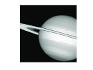
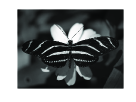
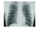
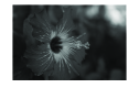
Figure 1: First row: Planet, Butterfly and Chest X-Ray images of sizes $512\times 512$, $448\times 600,$ and $592\times 728$ pixels, respectively. Second row: Flower, Spider Web and Artificial high resolution images from [18], all of size $1512\times 2264$ pixels.

The set of six grey intensity levels images used for illustrating the proposed HBW strategy are shown in Fig 1. The images in the first row: Planet, Butterfly and Chest X-Ray are of sizes $512\times 512$, $448\times 600$ and $592\times 728$ pixels. The images in the second row: Flower, Spider Web and Artificial are high resolution images taken from [18]. The Spider Web and Artificial are both only fractions of the much larger images in [18], which we have cropped to the same size as the Flower, i.e., $1512\times 2264$ pixels.

All the images of Fig. 1 are approximated in both, the intensity and wavelet domains by partitions of $8\times 8$ pixels. The transformed image is obtained using the CDF97 WT. The sparsity of an approximation is measured by the Sparsity Ratio (SR) defined as $\text{SR}=\frac{N_{x}N_{y}}{K}$, with $N_{x}N_{y}$ the total number of pixels and $K$ the number of nonzero coefficients to approximate the whole image.

I	MP	HBW	OMP	HBW	WT	DCT
P	28.1	29.0	30.4	31.0	40.7	27.1
B	10.6	11.2	12.3	12.7	9.6	10.7
C	22.6	23.2	23.6	24.4	34.2	20.7
F	41.0	42.8	42.6	43.9	119.5	40.0
S	34.8	35.7	36.5	37.0	70.0	33.5
A	26.4	27.5	29.7	30.7	24.9	19.4

TABLE I: SR resulting from approximating (in the intensity domain) the six images of Fig. 1, up to PSNR=45.0dB, by the methods: MP, OMP, their corresponding HBW versions, WT and DCT.

I	MP	HBW	OMP	HBW	WT	DCT
P	39.1	53.0	43.9	62.9	40.7	27.1
B	10.6	12.0	12.7	14.4	9.6	10.7
C	32.5	53.2	35.0	60.7	34.2	20.7
F	48.6	156.6	50.5	181.5	119.5	40.0
S	41.1	87.9	43.3	99.2	70.0	33.5
A	25.0	30.1	28.4	35.0	24.9	19.4

TABLE II: Same description as in Table 1 but in this case MP, OMP and the corresponding HBW versions are implemented in the wavelet domain. The results of the WT and DCT are repeated here to facilitate the comparison.

The approximation of all the images is carried out to achieve the required PSNR of 45.0dB using the above defined RDCDB dictionary and the greedy strategies OMP, MP and their corresponding HBW versions. The SRs arising when these techniques are implemented in the intensity domain are displayed in the first four columns of Table 1. The rows, from top to ground, correspond to the Planet (P), Butterfly (B), Chest (C), Flower (F), Spider Web (S) and Artificial (A) images (I). For comparison purposes, the results produced by conventional WT and DCT approaches are displayed in the last two columns of the table. The WT results are obtained by applying the CDF97 WT, on the whole image, and reducing coefficients by iterative thresholding until the PSNR of 45.0dB is reached. The results from the orthogonal DCT are obtained, from a partition of $8\times 8$ pixels, also by thresholding of coefficients.

From Table 1 it is clear that: a) Except for the Butterfly and Artificial images, in the intensity domain the results produced by a conventional WT approach significantly over perform the other approaches. b) Whilst the block independent OMP and MP methods produce smaller SRs than their corresponding HBW versions, the difference is not very significant. However, as can be observed in Table 2, all this is reversed if the greedy techniques are implemented with the RDCDB dictionary but in the wavelet domain. In this domain: a) for all the images the HBW versions of MP and OMP, with the simple RDCDB dictionary, significantly over-perform conventional WT and DCT approaches. b) Except for the Butterfly and Artificial images the difference in the SR produced by the HBW approaches, with respect to the block independent versions, is massive.

Putting aside the Butterfly and Artificial images, the common feature of the other images in Fig. 1 is the very significant difference in the SR produced by a conventional WT approximation, with respect to the conventional DCT. This is an indication that the representation of the images is particularity sparse in the wavelet domain. It is clear from Table 2 that, the sparser the approximation by the WT is, the lower the performance of OMP with respect to the proposed HBW version.

Finally, some information with regard to processing times is relevant. The tests presented here were run on a laptop with a 2.2 GHz Intel Processor and 3GB of RAM. The processing time (average of 10 independent runs in Matlab) for approximating the first three images of Fig 1 in the wavelet domain are: For the Planet 2.04 secs with OMP and 2.78 secs with HBW-OMP. For the Butterfly 7.13 and 11.56 secs and for the Chest 4.3 and 5.1 secs, respectively. Using a C++ MEX file for both approaches the corresponding times are reduced up to ten times. Thus, the larger images (second row of Fig 1) were approximated using MEX files. The running times corresponding to those images (left to right) are 5.71, 5.93 and 6.3 secs with OMP and 6.76, 9.7 and 21.9 secs with HBW-OMP.

In order to reduce processing time, the approximation of a large image can be realized by dividing the image into segments to be processed independently. Since each of the segments will contain different information, the sparsity of the segments may differ from one another. For comparison with the approximation of the whole image at once, it is necessary to make uniform the sparsity of all the segments. A possible way of achieving this is to randomize the position of the blocks in the whole image, to ensure that each segment contains blocks from different regions of the image. The implementation is carried out as follows: i) Perform a random permutation of the small blocks in the transformed domain. ii) Divide the resulting image into segments. iii) Apply HBW-OMP to each segment. iv) Place the blocks back in the original position.

Through this simple procedure and taking 12 segment of $540\times 560$ pixels each, the time to approximate the Artificial image is reduced to 6.1 secs while the PSNR does not change significantly (45.0dB).

V Conclusions

An approach, for HBW implementation of greedy methodologies operating on partitions, has been proposed. The proposal was motivated by the convenience of approximating some images in the wavelet domain. Certainly, if the image is characterized by having large smooth regions, for instance, when approximated in the intensity domain blocking artifacts are likely to be noticeable, even at high PSNR. Additionally, if an image is compressible in the wavelet domain, it can be expected to have a sparser approximation in that domain. This was illustrated through the OMP and MP methodologies. The numerical examples were chosen to enhance the fact that, for images which are highly compressible in the wavelet domain, approximations by partitions in such a domain may achieve much higher sparsity, provided that the proposed HBW version of greedy pursuit strategies is applied.

Acknowledgements

We are sincerely grateful to the Referees for their constructive criticism which has been of much help to present the proposal in the present form.

Support from EPSRC UK is acknowledged. The MATLAB and C++ MEX files for implementation of HBW-OMP with a separable dictionary (HBW-OMP2D) are available on [19] (section Examples).

References

- [1] J. Mairal, M. Eldar and G. Sapiro, “Sparse Representation for Color Image Restoration”, IEEE Trans. Image Proces., 17, 53 – 69 (2008).
- [2] M. Elad, Sparse and Redundant Representations: From Theory to Applications in Signal and Image Processing, Springer (2010).
- [3] J. Wright, Yi Ma, J. Mairal, G. Sapiro, T.S. Huang, and S. Yan, “Sparse Representation for Computer Vision and Pattern Recognition”, Proc. of the IEEE 98, 1031 – 1044 (2010).
- [4] J-L. Starck, F. Murtagh and J. M. Fadili, “Sparse Image and Signal Processing”, Cambridge University Press (2010).
- [5] Y. Yuan and D. M. Monro, “Improved matching pursuits image coding”, In ICASSP, 2, 201–204 (2005).
- [6] K. Skretting and K. Engan, “Image compression using learned dictionaries by RLS-DLA and compared with K-SVD”, ICASSP, 1517 – 1520 (2011).
- [7] R. Maciol, Y. Yuan and Ian T. Nabney, “Colour Image Coding with Matching Pursuit in the Spatio-frequency Domain”, ICIAP, Lecture Notes in Computer Science, 6978, 306–317 (2011).
- [8] J. Bowley and L. Rebollo-Neira, Sparsity and ‘Something Else’: An Approach to Encrypted Image Folding, IEEE Signal Processing Letters, 8, 189–192 (2011).
- [9] L. Rebollo-Neira, J. Bowley, A. Constantinides and A. Plastino, “Self contained encrypted image folding”, Physica A, 391, 5858–5870 (2012).
- [10] Y.C. Pati, R. Rezaiifar, and P.S. Krishnaprasad, “Orthogonal matching pursuit: recursive function approximation with applications to wavelet decomposition,” Proc. of the 27th ACSSC,1,40–44 (1993).
- [11] L. Rebollo-Neira and D. Lowe, “Optimized orthogonal matching pursuit approach”, IEEE Signal Process. Letters, 9, 137–140 (2002).
- [12] S. G. Mallat and Z. Zhang, “Matching Pursuits with Time-Frequency Dictionaries”, IEEE Trans. Signal Process., 41, 3397–3415 (1993).
- [13] Y. Eldar, P. Kuppinger and H. Biölcskei, “Block-Sparse Signals: Uncertainty Relations and Efficient Recovery”, IEEE Trans. Signal Process., 58, 3042–3054 (2010).
- [14] L. Rebollo-Neira and J. Bowley, “Sparse representation of astronomical images” Journal of The Optical Society of America A, Vol 30, 758–768 (2013).
- [15] M. Yaghoobi, T. Blumensath and M. E. Davies, “Dictionary learning for sparse approximations with the majorization method”, IEEE Trans. Signal Process., 109, 1– 14 (2009).
- [16] K. Skretting and K. Engan, “Recursive Least Squares Dictionary Learning Algorithm”, IEEE Trans. Signal Process., 58, 2121—2130 (2010).
- [17] I. Tos̆ić and P. Frossard, Dictionary Learning, IEEE Signal Process. Magazine, 28, 27–38 (2011).
- [18] http://www.imagecompression.info
- [19] http://www.nonlinear-approx.info