Classical scattering of charged particles confined on an inhomogeneous helix

Abstract

We explore the effects arising due to the coupling of the center of mass and relative motion of two charged particles confined on an inhomogeneous helix with a locally modified radius. It is first proven that a separation of the center of mass and the relative motion is provided if and only if the confining manifold represents a homogeneous helix. In this case bound states of repulsively Coulomb interacting particles occur. For an inhomogeneous helix, the coupling of the center of mass and relative motion induces an energy transfer between the collective and relative motion, leading to dissociation of initially bound states in a scattering process. Due to the time reversal symmetry, a binding of the particles out of the scattering continuum is thus equally possible. We identify the regimes of dissociation for different initial conditions and provide an analysis of the underlying phase space via Poincaré surfaces of section. Bound states inside the inhomogeneity as well as resonant states are identified.

The formation of helical patterns and structures is common in many natural systems ranging from DNA molecules and amino-acids to non-neutral plasmas trapped in magnetic fields Totsuji88 and self-assembled configurations of charged particles confined in nanotubes Vernizzi09 . Studying the motion of particles confined in a helix has proven to be a useful tool for the understanding of complex phenomena such as the optical activity of sugar solutions Desobry73 ; Dufey06 . Certainly the problem of the confined motion of particles in a helical manifold is of fundamental interest since it reveals many intriguing phenomena. Quantum particles confined in one dimension (1D), preserve some information of the surrounding 3D space and thus experience an effective geometric potential which depends on the curvature of the confining manifold Costa81 . Such geometric potential effects lead to the formation of bound states in helical waveguides with a locally modified radius Exner07 or in twisting tubes Goldstone92 . In the presence of an electric field, super-lattice properties can emerge for a confined charge carrier Kibis05 , whereas when the particles interact with dipolar forces a peculiar quantum phase transition from liquid to gas has been predicted Law08 .

In spite of their physical interest, helical traps have only recently been investigated experimentally. In nanotechnology, curved nanotubes such as rolls, spirals and helices from thin solid films of silicon-germanium can be constructed Prinz00 ; Schmidt01 . Helical traps can also be realized experimentally for cold atoms either via the interference of counter-propagating Laguerre-Gaussian beams Bhatt07 ; Okulov12 ; Vargas10 or via the evanescent field of a nanofiber Vetsch10 ; Vetsch12 ; Reitz12 which creates a double-helix trapping potential. Such setups allow the creation of a homogeneous helical potential over the entire length of the nanofiber as well as local modifications of the radius and the pitch of the helix through local variations of the diameter of the nanofiber Reitz12 . Beyond these, a plethora of trapping techniques also exist for (ultra-) cold ions Paul90 ; Schneider10 .

Motivated by the above, it is instructive to explore the classical behaviour of ions or generally charged particles in a helical geometry. Surprisingly this problem has not been studied extensively in the literature. In ref. Schmelcher11 it has been shown that the classical dynamics of a system of identical charged particles confined in a helical manifold presents very intriguing phenomena when the particles interact via long-range interactions such as the Coulomb interaction. In particular, the interplay between the 1D confined motion of the particles and their interactions via the full 3D space gives rise to an effective oscillatory force. This fact yields, in turn, stable equilibrium configurations despite the repulsive interactions between the particles and induces classical bound states whose number can be tuned by varying the parameters of the helix.

Following the direction of the above study, we explore in the present work the two-body scattering dynamics off an inhomogeneity in a helical trap. As a first step we rigorously prove that a separation of the center of mass (CM) and the relative motion is provided for an interaction potential which depends exclusively on the Euclidean distance between the particles $V(\left|\mathbf{r}_{1}-\mathbf{r}_{2}\right|)$, if and only if the confining curve is a homogeneous helix. Then, we examine the case of an inhomogeneous helical trap with a locally modified radius, and explore effects due to the coupling of the CM and relative motion. It is shown that initially bound states can finally dissociate due to the modulation of the potential which leads to an energy transfer between the CM and the relative degrees of freedom. Due to time reversal symmetry, it is thus equally possible for two unbound charged particles to form a bond due to the local inhomogeneity. A phase space analysis provides us with bound states within the inhomogeneous region as well as with resonant states and completes the picture of the two-particle dynamics.

The paper is organized as follows. In Sec. II we present the general Lagrangian for the problem of two interacting classical charged particles confined on a curve and we investigate the properties that the confining curve has to fulfill so that a separation of the CM and the relative degrees of freedom is provided. In Sec. III we present our model of two charged particles confined to an inhomogeneous helix. Section IV contains our results for the scattering, whereas section V provides our analysis of the respective phase space. Finally, Sec. VI represents a brief summary of our findings.

II. INTERACTING PARTICLES CONFINED TO A CURVED 1D-MANIFOLD

We consider a system of two particles with masses $m_{1},m_{2}$, interacting via a potential $V(\left|\mathbf{r}_{1}-\mathbf{r}_{2}\right|)$ that depends only on the Euclidean distance between them. Their Lagrangian is given by

$$L(\{\mathbf{r}_{i},\dot{\mathbf{r}}_{i}\})=\frac{1}{2}\sum_{i=1}^{2}m_{i}{\dot{\mathbf{r}}_{i}}^{2}-V(\left|\mathbf{r}_{1}-\mathbf{r}_{2}\right|).$$

If the particles are confined onto a smooth, regular and either closed or infinitely extended space curve $\mathbf{r}:\mathbb{R}\mapsto\mathbb{R}^{3}$ parametrized with the arbitrary parameter $u$, i.e. $\mathbf{r}_{i}=\mathbf{r}(u_{i})$, the Lagrangian takes the form

$$L(\{u_{i},\dot{u}_{i}\}) = \frac{1}{2}\sum_{i=1}^{2}m_{i}\left|\partial_{u_{i}}\mathbf{r}(u_{i})\right|^{2}\dot{u}_{i}^{2}$$ (1)

$$- V(\left|\mathbf{r}(u_{1})-\mathbf{r}(u_{2})\right|).$$

If we choose the arc length parametrization footnote

$$s:u\mapsto s(u)=\int_{0}^{u}\left|\partial_{u^{\prime}}\mathbf{r}(u^{\prime})\right|du^{\prime},$$ (2)

since the tangent vector $\mathbf{t}(s_{i})=\partial_{s_{i}}\mathbf{r}(s_{i})$ is a unit vector we arrive at the expression

$$L(\{s_{i},\dot{s}_{i}\})=\frac{1}{2}\sum_{i=1}^{2}m_{i}\dot{s}_{i}^{2}-V(\left|\mathbf{r}(s_{1})-\mathbf{r}(s_{2})\right|).$$ (3)

We thus observe that the kinetic energy term retains the Cartesian form in the arc length parametrization, leading to the familiar expressions for the conjugate momenta and the Euler-Lagrange (EL) equations of motion. Introducing the CM $S=(m_{1}s_{1}+m_{2}s_{2})/(m_{1}+m_{2})$ and the relative coordinate $s=s_{1}-s_{2}$, as well as the total mass $M=m_{1}+m_{2}$ and the reduced mass $\mu=\frac{m_{1}m_{2}}{M}$, we are led to

$$L(\{s,S,\dot{s},\dot{S}\})=\frac{1}{2}M\dot{S}^{2}+\frac{1}{2}\mu\dot{s}^{2}-\tilde{V}\left(S,s\right),$$ (4)

where

$$\tilde{V}(S,s)=V\left(\left|\mathbf{r}(S+\frac{m_{2}}{M}s)-\mathbf{r}(S-\frac{m_{1}}{M}s)\right|\right).$$ (5)

This yields the following EL equations

$$M\ddot{S}=-\frac{\partial\tilde{V}}{\partial S},~{}\mu\ddot{s}=-\frac{\partial\tilde{V}}{\partial s}.$$ (6)

Evidently, a separation of the CM from the relative motion is provided if and only if $\frac{\partial\tilde{V}}{\partial S}$ is exclusively a function of $S$ which is equivalent to

$$\frac{\partial^{2}\tilde{V}}{\partial s\partial S}=0\Leftrightarrow\tilde{V}(S,s)=V_{1}(S)+V_{2}(s)$$ (7)

with $V_{1},V_{2}$ being arbitrary functions of $S$ and $s$ respectively.

In order to analyze this condition further, we technically have to distinguish the two cases of a regular and a singular potential $\tilde{V}(S,s)$ at $s=0$.

For a regular potential, we obtain from (5) that $\tilde{V}(S,0)=V(0)$. Condition (7) then yields

$$V_{1}(S)=V(0)-V_{2}(0)=const.\Rightarrow\frac{\partial V_{1}}{\partial S}=\frac{\partial\tilde{V}}{\partial S}=0.$$

For a potential with a singularity at $s=0$, as in the typical case of Coulomb interaction, choosing an infinitesimal value $\varepsilon>0$ for the $s$ coordinate, we are led through (5) to

$$\tilde{V}(S,\varepsilon) = V\left(\left|\mathbf{r}(S+\frac{m_{2}}{M}\varepsilon)-\mathbf{r}(S-\frac{m_{1}}{M}\varepsilon)\right|\right)$$ (8)

$$= V\left(\left|\mathbf{r}(S)+\frac{m_{2}}{M}\varepsilon\mathbf{t}(S)-\mathbf{r}(S)+\frac{m_{1}}{M}\varepsilon\mathbf{t}(S)\right|\right)$$

$$= V\left(\left|\varepsilon\mathbf{t}(S)\right|\right)=V\left(\varepsilon\right),$$

since $\left|\mathbf{t}(S)\right|=1$. Thus, for arbitrary $S,\tilde{S}$

$$\tilde{V}(S,\varepsilon)=\tilde{V}(\tilde{S},\varepsilon)=V(\varepsilon)$$

and Eq. (7) for $s=\varepsilon$ leads to

$$V_{1}(S)=V_{1}(\tilde{S})=V(\varepsilon)-V_{2}(\varepsilon)~{}\forall S,\tilde{S}~{}\Rightarrow\frac{\partial V_{1}}{\partial S}=\frac{\partial\tilde{V}}{\partial S}=0.$$

Therefore both cases lead to the condition $\frac{\partial\tilde{V}}{\partial S}=0$ and we conclude that the CM and relative motion mutually separate for a potential that depends only on the inter-particle Euclidean distance (Eq. (5)) if and only if $\frac{\partial\tilde{V}}{\partial S}=0$. Furthermore, this is a necessary and sufficient condition for the conservation of the total momentum

$$P=\frac{\partial L}{\partial\dot{S}}=M\dot{S}$$

as follows from (4) and the EL equations (6), yielding a free particle motion for the CM.

Introducing the function $R(s_{1},s_{2})=\left|\mathbf{r}(s_{1})-\mathbf{r}(s_{2})\right|$, with $s_{1}=S+\frac{m_{2}}{M}s$, $s_{2}=S-\frac{m_{1}}{M}s$ and $V^{\prime}(R)=\frac{dV}{dR}\big{|}_{R=R(s_{1},s_{2})}$ we obtain

$$\frac{\partial\tilde{V}}{\partial S} = V^{\prime}(R)\frac{\partial R}{\partial S}$$

$$= V^{\prime}(R)(\partial_{s_{1}}R(s_{1},s_{2})+\partial_{s_{2}}R(s_{1},s_{2}))$$

and we are thus led to the conclusion that a conservation of the total momentum as well as a separation of the CM from the relative coordinate is provided for interacting particles if and only if

$$\frac{\partial R}{\partial S}=\partial_{s_{1}}R(s_{1},s_{2})+\partial_{s_{2}}R(s_{1},s_{2})=0,~{}\forall s_{1},s_{2}\in\mathbb{R}.$$ (10)

The results of Schmelcher11 indicate that for the confining manifold being a homogeneous helix, i.e. a helix with a constant radius and pitch, the CM motion is separated from the relative one. In fact, the homogeneous helix - including also the limiting cases of the straight line and the circle - is the only curve allowing for such a separation, as follows from the proposition below.

Proposition: Condition (10) holds for a smooth, regular curve $\mathbf{r}(s)$ that is either closed or extends to infinity and is parametrized by its arc length $s\in\mathbb{R}$ if and only if the curve is a homogeneous helix.

The proof of this proposition is provided in the Appendix.

III. TWO CHARGED PARTICLES IN AN INHOMOGENEOUS HELICAL TRAP

In the following we study the classical dynamics of two identical charged particles confined in a modified helix. The modification consists of a hump, i.e. a local change of Gaussian form in the radius (Eq. (12)). The interaction between the particles is given by a repulsive Coulomb potential

$$V(\left|\mathbf{r}_{1}-\mathbf{r}_{2}\right|)=\frac{\lambda}{\left|\mathbf{r}_{1}-\mathbf{r}_{2}\right|},$$

with $\lambda>0$. We explore in particular the effects due to the coupling of the CM and relative motion in the presence of the helical hump.

The inhomogeneous helix parametrized by the angle parameter $u$ is given by:

$$\mathbf{r}(u)=(R(u)\cos(u),R(u)\sin(u),\frac{h}{2\pi}u)$$ (11)

with

$$R(u)=1+\epsilon\exp[-cu^{2}],$$ (12)

where both the modified radius $R(u)$ and the pitch of the helix $h$ have been scaled with the radius of the corresponding uniform helix $R_{0}$. We use for the inhomogeneous helix the parameter values $\epsilon=1,~{}c=0.01,~{}h=0.4\pi$. Figure 1 depicts the shape of such a helix and the localized radial modulation.

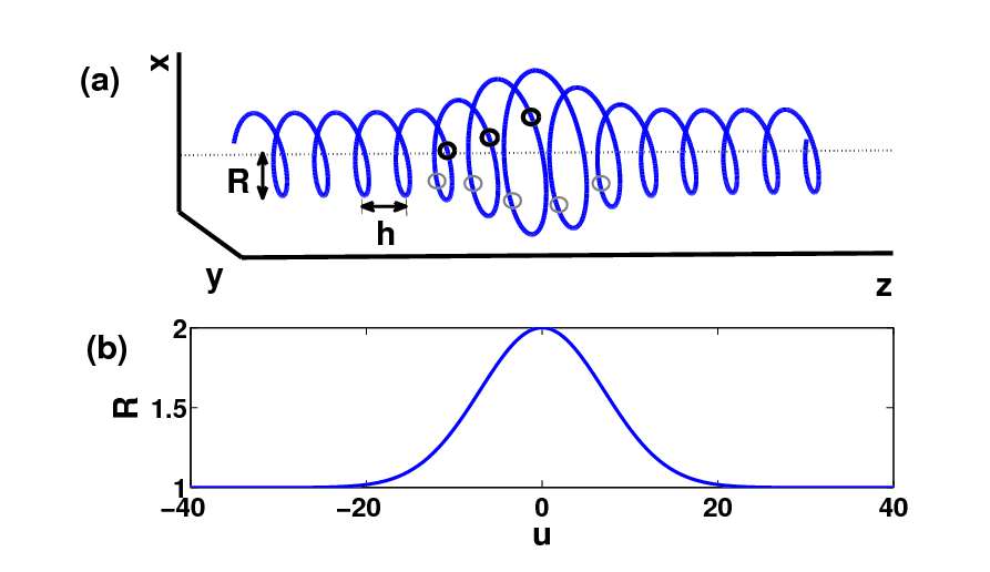
Figure 1: (color online). (a) Helix with a local modification of the radius $R(u)$ and a pitch $h$, as given by Eq. (11). (b) Local modulation of the radius as a function of the parameter $u$.

Since the particles are identical, $m_{i}=m$, we can choose dimensionless units by rescaling all quantities with $m$, $\lambda$ and $R_{0}$, i.e. introducing $\tilde{m}=\tilde{\lambda}=1$ and

$$\tilde{x}=\frac{x}{R_{0}},~{}\tilde{t}=t\sqrt{\frac{\lambda}{mR_{0}^{3}}},~{}\tilde{H}=\frac{HR_{0}}{\lambda},~{}\tilde{p}=p\sqrt{\frac{R_{0}}{m\lambda}}$$

In the following we omit for simplicity the tilde.

Performing then a Legendre transformation with $p_{i}=\frac{\partial L}{\partial\dot{u}_{i}}$ we obtain from (1) the Hamiltonian

$$H(\{u_{i},p_{i}\})=\frac{1}{2}\sum_{i=1}^{2}\frac{p_{i}^{2}}{(\partial_{u_{i}}\mathbf{r}(u_{i}))^{2}}+\frac{1}{\left|\mathbf{r}(u_{1})-\mathbf{r}(u_{2})\right|}$$ (13)

From this we deduce the equations of motion $\dot{u}_{i}=\frac{\partial H}{\partial p_{i}},\dot{p}_{i}=-\frac{\partial H}{\partial u_{i}}$, which we solve numerically for different initial conditions with a Runge-Kutta method of fourth-fifth order with a variable time step size (ODE45). In order to study the dynamics in terms of CM and relative motion, it is desirable to have a Hamiltonian with a kinetic energy term of Cartesian form. This is achieved under the arc length parametrization (2) and leads to

$$H(\{s_{i},\dot{s}_{i}\})=\frac{1}{2}\sum_{i=1}^{2}\dot{s}_{i}^{2}+\frac{1}{\left|\mathbf{r}(s_{1})-\mathbf{r}(s_{2})\right|}.$$

The $s_{i}$ are obtained (numerically) via Eq. (2). Introducing CM $S=\frac{s_{1}+s_{2}}{2}$ and relative coordinates $s=s_{1}-s_{2}$ yields the Hamiltonian

$$H(S,s,\dot{S},\dot{s})=\dot{S}^{2}+\frac{\dot{s}^{2}}{4}+\frac{1}{\left|\mathbf{r}(u_{1}(S,s))-\mathbf{r}(u_{2}(S,s))\right|}$$ (14)

and the corresponding equations of motion:

$$\ddot{S} = -\frac{1}{2}\frac{\partial}{\partial S}\frac{1}{\left|\mathbf{r}(u_{1}(S,s))-\mathbf{r}(u_{2}(S,s))\right|}$$

$$\ddot{s} = -2\frac{\partial}{\partial s}\frac{1}{\left|\mathbf{r}(u_{1}(S,s))-\mathbf{r}(u_{2}(S,s))\right|}.$$ (15)

We clearly observe here the coupling between $S$ and $s$ in the potential term. In the case of the uniform helix Schmelcher11 the arc length integral can be solved analytically and the Hamiltonian can be written explicitly as:

$$H(s,\dot{S},\dot{s})=\dot{S}^{2}+\frac{\dot{s}^{2}}{4}+\frac{1}{\sqrt{2\left(1-\cos(\frac{s}{a})\right)+(\frac{h}{2\pi a})^{2}s^{2}}},$$ (16)

with $a=\sqrt{1+\left(\frac{h}{2\pi}\right)^{2}}$.

For understanding the dynamics it is crucial to analyze the properties of the potential $V(S,s)$. Obviously, we have $\lim_{R\rightarrow\infty}V(R)=0$. We focus first on the uniform helix for which $V=V(s)$ (see Eq. (16)) and thereafter we consider the case of the coupling of the CM and relative motion. Figure 2 below shows the behaviour of this potential curve for $s<20$. We identify three potential wells which can support bound states and become shallower as $s$ increases.

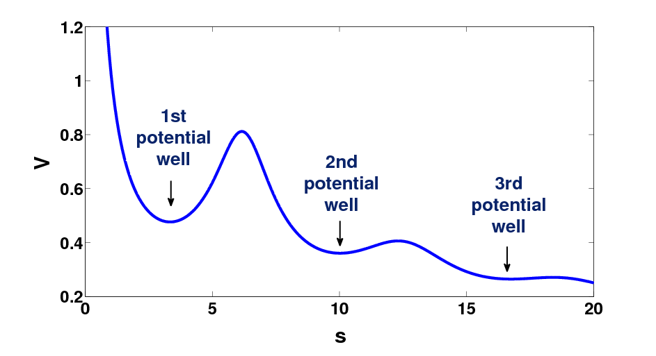
Figure 2: (color online). Potential curve for the uniform helix with parameters $h=0.4\pi$ and $R=1$. We observe three potential wells located at $s=3.34,10.00$ and $16.75$ with minimum values $V=0.48,0.36$ and $0.26$ respectively.

The potential $V(S,s)$, taking into account the hump, is illustrated in Fig. 3. Since it depends on both the CM $S$ and the relative $s$ coordinate, it represents a two-dimensional potential landscape.

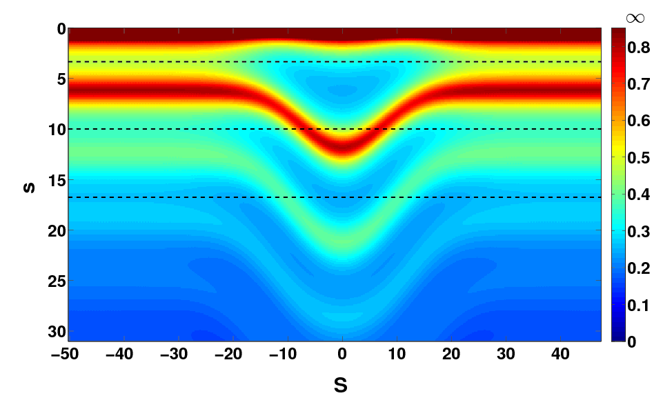
Figure 3: (color online). Contour plot of the potential $V(S,s)$ for the inhomogeneous helix. The dashed lines represent the positions of the minima of the three wells for the homogeneous case. The effect of the local modification of the radius is evident for $\left|S\right|\lesssim 30$.

We clearly observe two regions with a distinct behaviour. The first, for large values of the CM coordinate $\left|S\right|\gtrsim 30$, presents a uniform behaviour, approximately independent of $S$. It is affected only by the relative coordinate $s$ in the same way as the potential of the homogeneous helix (Fig. 2), thereby presenting three wells for $\left|s\right|\approx 3,10,17$. In this uniform domain the CM and the relative motion are thus decoupled. The second region, for $\left|S\right|\lesssim 30$, presents a strong dependence on the CM coordinate and thus constitutes a regime of strong coupling. The reader should note that the arc length (2) is taken w.r.t. the centre of the hump and consequently regions with small $S,s$ correspond to small $s_{i}$ and lie in the inhomogeneous region of the helix.

Two effects are evident: each potential well becomes deeper and the contour lines bend in the regime of the inhomogeneity. Concerning the potential barriers, their maximum value decreases by $\sim 8\%$ at the sides of the inhomogeneous region, whereas for $S\approx 0$ it retains the value of the homogeneous regime. All these effects can be explained by the modulation of the radius of the helix as discussed below.

Modulation of the radius and potential landscape. Since the pitch of the helix is much smaller than its circumference $(h<2\pi R)$ in both the homogeneous and the inhomogeneous regime, the maximum and the minimum potential configurations occur for approximately constant values of the relative angle parameter $\tilde{u}=u_{1}-u_{2}$, namely for $\tilde{u}_{max}=2k\pi$ and $\tilde{u}_{min}=(2k-1)\pi,~{}k\in\mathbb{Z}$ Schmelcher11 , which for the first well ($k=1$) correspond respectively to particles separated by one or half a winding of the helix (Fig. 4). The Euclidean distance between the particles at the minimum configuration increases substantially with the increment of the radius (Fig. 4 (b), (c)), reaching its maximum value at $S\approx 0$ (Fig. 4 (c)) thereby resulting in a strong increase of the potential depth.

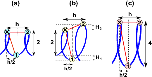
Figure 4: (color online). Euclidean distances of the particles for the minimum $(\mbox{\footnotesizex⃝},\mbox{\tiny1⃝})$ and the maximum $(\mbox{\footnotesizex⃝},\mbox{\tiny2⃝})$ potential configurations of the first potential well for three different regions of the inhomogeneous helix: (a) the uniform domain of the helix with pitch $h$ and radius $R=1$, (b) the left side of the inhomogeneous region where the radius increases by $H_{1}$ at the bottom and by $H_{2}$ at the top, whereas the pitch remains the same, (c) the central part of the inhomogeneous domain $S\approx 0$, which since the modulation of the radius is stationary can be approximately treated as a part of a uniform helix with the same pitch $h$, but double radius $R=2$.

For the maximum configurations, the Euclidean distance increases as well off the centre of the inhomogeneous region but, as it is shown in Fig 4 (b), this increment is small compared to that of the minimum configuration. At $S\approx 0$, the rate of change of the radius becomes small enough for the radius to be considered constant with twice the value of its homogeneous asymptotics (Fig. 4 (c)). However the pitch $h$ remains the same, resulting in the same Euclidean distance between the particles of the maximum configuration and thus leading to the same maximum potential values as that of the uniform domain (Fig. 4 (c)). The generalization to other potential wells (second, third) is evident in the regime $S\approx 0$: for the case of the maximum configuration both particles are shifted by the same distance in the same direction whereas for the case of the minimum configuration by the same distance in opposite directions. This fact results both in an unaltered maximum value of the potential barrier and in a considerable increase of the potential depth.

Finally we note that the contour lines of the potential bend inside the inhomogeneity towards larger $s$ values as compared to the uniform domain. This effect is more pronounced for larger relative distances, i.e for the third well as shown clearly in Fig. 3.

In the following sections we will not discuss the dynamics of the system in terms of the trajectories $t\mapsto s_{i}(t)$ of two individual particles but rather in terms of that of a fictitious particle with two degrees of freedom - $S$ and $s$ - moving in the 2D potential of Fig. 3. This interpretation is suggested by the form of the Hamiltonian (14), which provides us with the respective equations of motion (15). Note however, that these two degrees of freedom have different effective masses, a fact that needs to be taken into account when investigating the dynamics of the fictitious particle in terms of the potential gradients in the CM and the relative direction.

IV. SCATTERING OFF THE HELICAL HUMP

We analyze now the scattering behaviour of a bound pair of charged particles confined in the inhomogeneous helix that has been described above. We assume that the particles start in the uniform domain, i.e. for $S\ll-30$ with $\dot{S}>0$. We introduce $S_{h}$ as the value of $\left|S\right|$ after which the helix as well as the potential are considered uniform. Specifically we choose $S_{h}\approx 35.6$ for which the radius is identical to that of the homogeneous helix within $0.1\%$. The particles are further assumed to be initially bound, so their relative coordinate $s$ lies within the region of one of the three wells discussed in Sec. IV. As they pass through the inhomogeneous region, energy is transfered between the CM and the relative degree of freedom due to the coupling. This transfer can lead to dissociation of the particles, which is reflected in the very low values of the interaction potential ($V\rightarrow 0$) at the end of the propagation (i.e. for $S\gg 30$).

We will initially discuss the case where the particles start with zero relative velocity $\dot{s}=0$ at the minimum of each of the three wells (Subsec. A) and then examine further the case of the first potential well for different initial conditions (Subsec. B).

A. Initial conditions with zero relative momentum

First potential well. The particles are placed in the homogeneous domain ($S\ll 0$) of the helix, in the minimum of the first potential well $s=3.34$ (Fig. 2), with $\dot{s}=0$. We vary the initial values of the CM kinetic energy $T_{S}=\dot{S}^{2}$, over several orders of magnitude. The different initial conditions are propagated for a time period $t=600$. After that time the particles have passed the region of inhomogeneity of the helix, the scattering process is in its asymptotic regime, and we can record the final values of the potential energy $V$, the relative energy $E_{s}=\frac{\dot{s}^{2}}{4}+V$, and the relative coordinate $s$. If the final value of $V$ lies within the first potential well, i.e. $0.48<V<0.81$, then the particles have remained bound, whereas if $V$ approaches zero they have dissociated through the scattering, which is also ensured by large values of the relative coordinate.

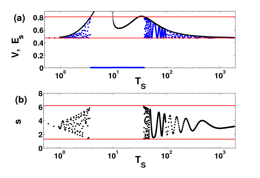
Figure 5: (color online) Overview of final bound and unbound states for initially bound states started in the first potential well: (a) Final potential values $V$ (blue dots) and final relative energy values $E_{s}$ (black dots) for different initial CM kinetic energies $T_{S}$. The red lines represent the boundary potential values (minimum of well, maximum of barrier) of the first potential well. (b) Final relative coordinate values $s$ (black dots) for different initial CM kinetic energies $T_{S}$. The red lines represent the boundary values of those $s$ which lie within the first potential well.

We clearly observe in Fig. 5 (a) two regimes of finally bound configurations: $0\leq T_{S}\leq 3.83$ and $T_{S}\geq 38.86$, separated by a region of dissociation $3.83\leq T_{S}\leq 38.86$. For small $T_{S}$, below a critical value $T_{S_{c1}}$ it is expected that an energy transfer between the CM and the relative degree of freedom would not provide sufficient energy so that the particle can overcome the potential barrier. After $T_{S_{c1}}\approx 3.83$ dissociation becomes possible and it indeed occurs. However, the dissociation regime stops at a second critical value $T_{S_{c2}}\approx 38.86$, a fact that although counterintuitive from the point of view of the possible energy supply, can be explained by the limited range of the inhomogeneous region ($\left|S\right|\leq 30)$. For very high CM velocities $\dot{S}$, the particles get through the inhomogeneity very fast, allowing for a very short interaction time only. The effect of the coupling is therefore very restricted, prohibiting a substantial energy transfer. In other words, the particles’ motion is almost unaffected by the presence of the hump due to their large velocities. In the regime of bound states the change of $T_{S}$ induces a change of the $s$-oscillation phase at the end of the propagation ($t=600$) leading to an oscillatory pattern of the final values of $V$ and $s$. Another interesting feature of Fig. 5 (a), is the behaviour of the final relative energy $E_{s}$. In the middle of the dissociation region, it acquires values less than that of the potential barrier $V_{max}\approx 0.81$, a fact that will be analyzed in Subsec. B.

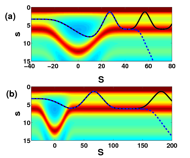
Figure 6: (color online) Finally bound (solid black line) and dissociated (dashed blue line) trajectories near: (a) the first transition point $T_{S_{c1}}\approx 3.83$, (b) the second transition point $T_{S_{c2}}\approx 38.86$. The trajectories in each case ((a),(b)) differ in their CM velocities only by $0.001$.

Let us next explore the behaviour of the trajectories for $T_{S}$ close to the critical values $T_{S_{c1}},T_{S_{c2}}$ which will be referred to in the following as transition points. Our results are presented in Fig. 6. In both cases (Figs. 6 (a),(b)) a sharp transition from a bound to a dissociated final state occurs when $T_{S}$ is fine tuned. This is depicted in the form of the corresponding trajectories which are essentially on top of each other for $S$ less than a critical value $S_{c}$. This value is much larger for the second transition point with $T_{S_{c2}}>T_{S_{c1}}$, a fact that can be attributed to the larger value of the CM velocity. There is an evident transfer of energy to the relative degree of freedom depicted in the very large amplitude of the $s$-oscillation of the fictitious particle for bound trajectories, after the scattering. With a slight increment of this transfer the states dissociate after an oscillation. The trajectory of the fictitious particle is deflected inside the hump following the curved topology of the potential landscape until it comes across a large value of the potential barrier where it becomes reflected backwards. From then on, it continues its regular path in the right homogeneous domain without any further energy transfer. As expected, the motion of the particle is much less affected (smaller angle of deflection) by the presence of the inhomogeneity for larger CM velocity (Fig. 6 (b)) due to its inertia.

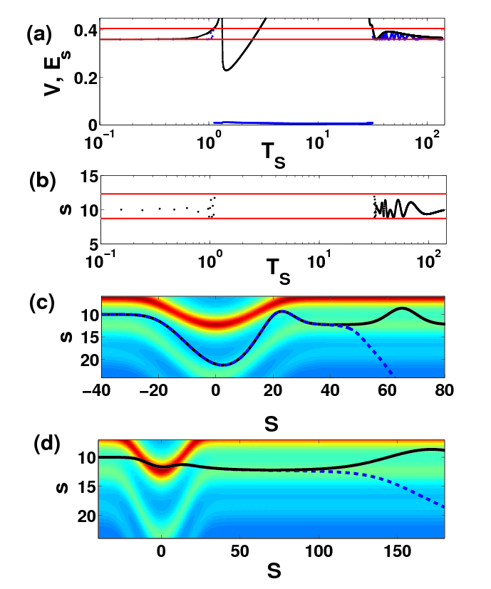
Figure 7: (color online) (a)-(b) Same as in Fig. 5, but for particles starting in the second potential well. (c)-(d) Same as in Fig. 6 but with: (c) $T_{S_{c1}}\approx 1.15$, (d) $T_{S_{c2}}\approx 33.54$.

Second potential well. We now place the particles in the minimum of the second potential well $s=10.00$ (Fig. 2) at the left homogeneous region, with zero relative velocity. Varying the CM kinetic energy $T_{S}$ we observe again (Figs. 7 (a),(b)) a region of dissociation $1.15\leq T_{S}\leq 33.53$ surrounded by regions of bound states, yielding two transition points: $T_{S_{c1}}=1.15$ (Fig. 7 (c)) and $T_{S_{c2}}=33.53$ (Fig. 7 (d)). The dissociation region is overall shifted to lower values of $T_{S}$, compared to our previous results for the first potential well. From an energetical point of view, the shift of the first transition point $T_{S_{c1}}$ is expected since the potential barrier lowers, allowing for dissociation with less energy transfer. However, this argument alone would lead to a shift of $T_{S_{c2}}$ to larger values, contrary to what is observed here. The suppression of $T_{S_{c2}}$ seems to be a result of the bending of the potential landscape inside the hump. In particular, the straight line indicating the minimum of the second potential well in the homogeneous regime, passes through the first potential well close to its barrier (Fig. 3). Trajectories with high enough CM kinetic energy $T_{S}\geq T_{S_{c2}}$, encounter this barrier and are forced to crest it (Fig. 7 (d)), a fact that reduces abruptly the amount of the energy transfer and leads to extended binding. This effect is more pronounced in the case of the third potential well as discussed below.

Third potential well. Similarly to the previous cases, we now place the particles in the minimum of the third potential well $s=16.75$ (Fig. 2) at the left homogeneous region, again with $\dot{s}=0$. A variation of the CM kinetic energy $T_{S}$ (Figs. 8 (a), (b)), provides us surprisingly with two distinct dissociation regimes $0.46\leq T_{S}\leq 3.76,~{}5.59\leq\dot{S}\leq 70.35$, separated by a small region of bound states ($3.76\leq T_{S}\leq 5.59$), leading to four transition points $T_{S_{c1}}=0.46,~{}T_{S_{c2}}=3.76,~{}T_{S_{c3}}=5.59,~{}T_{S_{c3}}=70.35$ (Figs. 8 (c)-(f)).

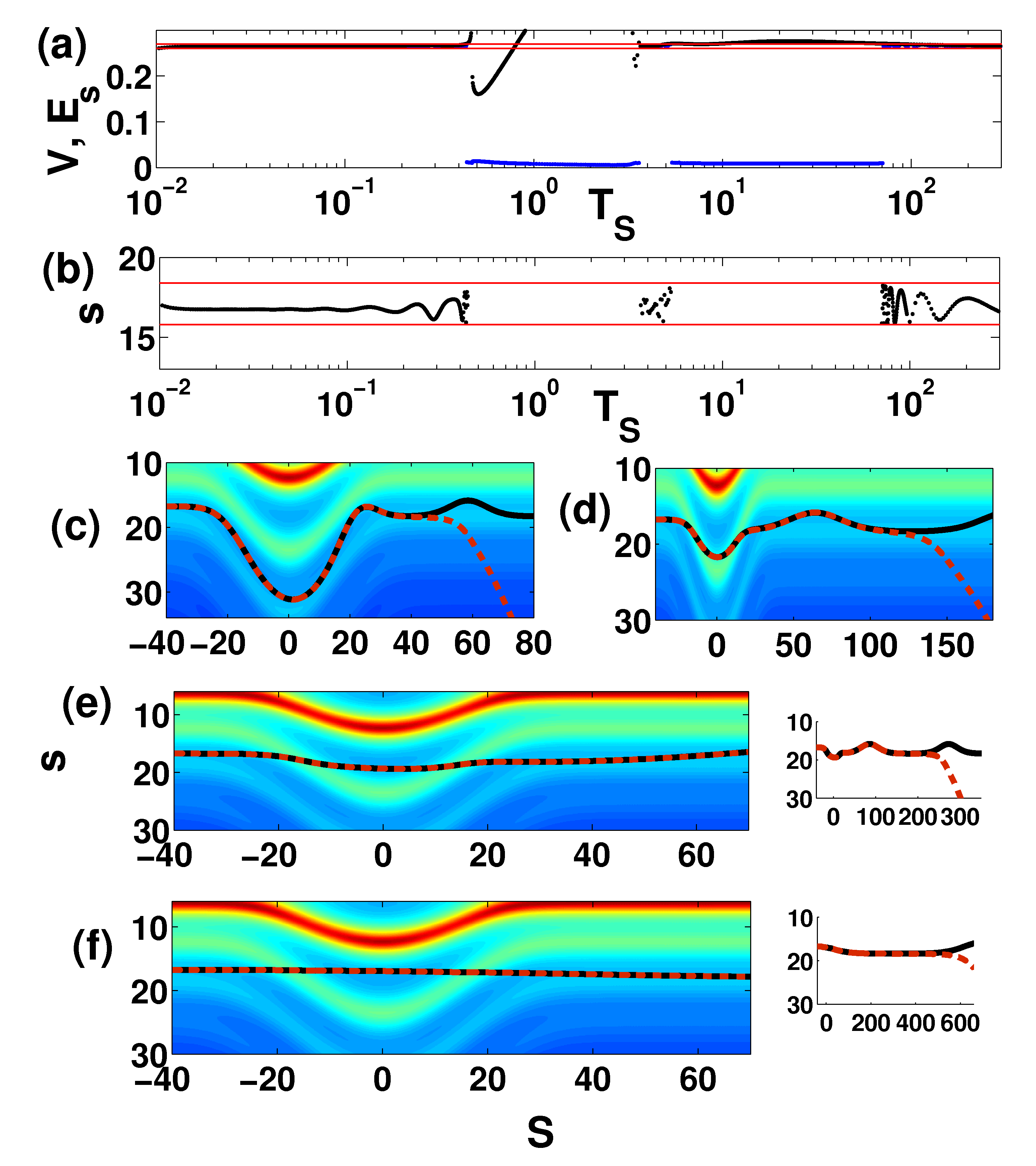
Figure 8: (color online) (a)-(b) Same as in Fig. 5, but for particles starting in the third potential well. (c)-(f) Same as in Fig. 6 but with: (c) $T_{S_{c1}}\approx 0.46$, (d) $T_{S_{c2}}\approx 3.76$, (e) $T_{S_{c3}}\approx 5.59$, (f) $T_{S_{c4}}\approx 70.35$. The small subfigures in (e) and (f) present the respective trajectories for large values of $S$, following them up to the point where the dissociative and bound trajectories separate from each other.

This fact is a direct result of the bending of the potential landscape, which affects mainly the larger relative coordinates $s$, i.e. the third well. In particular, as depicted in Fig. 3 the straight line of the minimum of the third potential well, passes, inside the hump, above the minimum of the second potential well. Due to the shallowness of the third potential well, only a very small amount of energy transfer $\sim 0.01$ is needed for the particles to overcome the barrier and dissociate, a fact that shifts the first transition point $T_{S_{c1}}$ to low values. When the fictitious particle has enough CM kinetic energy ($T_{s}\geq T_{S_{c2}}$), it crests the barrier of the second well, but since it gets directly deflected within it, it cannot reach its inner region and the minimum (Fig. 8 (d)). This is similar to the case of the second transition point of the second potential well (Fig. 7 (d)) and as in there, it is followed by a regime of bound states. However, if the CM velocity gets large enough ($T_{S_{c3}}=5.59$), the fictitious particle is less deflected and can reach the region of the minimum of the second potential well (Fig. 8 (e)), allowing for further energy redistribution between the two degrees of freedom. Thus, a second dissociation region occurs, which extends to very high values of $T_{S}\approx 70$, a fact that can also be attributed to the very small height of the potential barrier. Nevertheless, even this height cannot be overcome, when the fictitious particle acquires CM kinetic energy larger than $T_{S_{c4}}$, since the dwell time becomes very small, leading again to bound trajectories as in the cases of the other wells.

For this potential well, sharp transitions from a bound to an unbound state occur too at the four transition points as shown in Fig. 8(c)-(f). It is evident that at the fourth transition point with a large value of $T_{S}$, the motion of the fictitious particle is only slightly affected by the inhomogeneity, tending to a straight line (Fig. 8 (f)).

We emphasize that since the equations of motion of the system (Eq. (15)) possess a time reversal symmetry, the transitions from bound to unbound states can be directly mapped into transitions from free states to bound ones. The creation of bonds through scattering is surprising, especially in view of the fact that the particles interact via a repulsive Coulomb potential. For these reasons we find it interesting to examine this process further below.

B. Initial conditions with nonzero relative velocity in the first potential well.

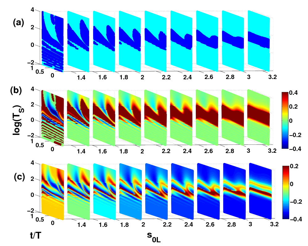
Figure 9: (color online) (a) States that after scattering remain bound (cyan regions) and states that are led to dissociation (blue regions), (b) color encoded values of the relative difference between the final and the initial maximum kinetic energy of the relative motion $(T^{s}_{max_{f}}-T^{s}_{max_{i}})/E_{s}$, (c) color encoded values of the difference between the final relative energy $E_{s_{f}}$ and the maximum value of the potential barrier of the first well $V_{max}$ for different $s_{0L}$ (X axis), $\frac{t}{T}$ (Y axis) and $\log(T_{S})$ (Z axis). Note that in case (b) the zero value is within the green region whereas in case (c) within the orange one.

We investigate now the scattering for arbitrary initial conditions, focusing on the first potential well. When the particles are in the uniform domain of the helix, inside the first well with a nonzero relative velocity, the fictitious particle performs an oscillation in the relative coordinate $s$. The phase of this oscillation when the fictitious particle enters the hump affects the energy transfer between the CM and the relative motion. Moreover, the value of the relative initial energy $E_{s}$ plays a crucial role in determining which states become dissociated, since states with higher $E_{s}$ require less amount of energy transfer in order to overcome the potential barrier. Thus, for a complete description of the scattering process, we need except from the initial center of mass kinetic energy $T_{S}$ to specify two other parameters, namely the initial relative energy and the phase of the relative oscillation.

For reasons of convenience we assume that the fictitious particle starts at a point $1.3<s_{0L}\leq s_{min}=3.34$ of the first potential well in the uniform domain with zero relative velocity $\dot{s}=0$. In other words $s_{0L}$ is the left turning point of the oscillation in the relative coordinate and is related to the total relative energy by $E_{s}=V(s_{0L})$, with $V$ being the potential of the homogeneous regime given by Eq. (16). We denote the right turning point for the same energy with $s_{0R}$.

We represent the phase of the oscillation, by the parameter $0\leq\frac{t}{T}<1$ which stands for the fraction of the period of the relative oscillation

$$T=2\int_{s_{0L}}^{s_{0R}}\frac{ds^{\prime}}{\sqrt{2(E_{s}-V(s^{\prime})})}$$

at which the particles enter the hump. In such a way $\frac{t}{T}=0$ corresponds to particles at $s_{0L}$ with $\dot{s}=0$ at the entrance point $S_{hL}=-S_{h}$, whereas $\frac{t}{T}=0.5$ corresponds to particles at $s_{0R}$ with $\dot{s}=0$. This parameter can be adjusted by changing the initial CM coordinate $S$ in the homogeneous region, while keeping $\dot{S}$ fixed. Due to our genuine interest in the scattering properties with varying phase, the absolute phase dependence induced by the arbitrariness of $S_{h}$ is rendered irrelevant.

Our results are presented in Fig. 9 for nine representative values of $s_{0L}$, ranging from energies close to the potential minimum ($s_{0L}\approx 3.3$) to close to the potential barrier height ($s_{0L}\approx 1.3$). Each such value produces a slice which imprints the dependence of the property under consideration on the other two parameters: $T_{S}$ and $\frac{t}{T}$.

Figure 9 (a) provides us with the finally bound and unbound states for the different initial conditions. For $s_{0L}\approx 3.3$, close to the minimum, we observe that the phase of oscillation $\frac{t}{T}$ does not affect the behaviour of the system, as expected, and we regain the results of Subsec. A with a single dissociation region of a rectangular shape for different CM kinetic energies $T_{S}$. The shape of this regime is deformed as we go to higher relative energies (smaller $s_{0L}$) and it develops a dip. By increasing further $E_{s}$ the dissociation area breaks into two parts for a certain regime of initial phases $\frac{t}{T}$, providing us with two dissociation regions with varying $T_{S}$. As we approach the threshold energy for passing the potential barrier ($s_{0L}\approx 1.3$) we observe an alternating sequence of bound and dissociation regions, even at very low CM kinetic energies. This is a surprising feature which makes the dissociation process sensitive to even small changes of the underlying parameters, such as the initial value of $T_{S}$ in the scattering process.

In Fig. 9 (b) we present our results for the relative amount of gain or loss of the maximum relative kinetic energy $(T^{s}_{max_{f}}-T^{s}_{max_{i}})/E_{s}$ through the scattering. Clearly the regions of high positive $(T^{s}_{max_{f}}-T^{s}_{max_{i}})/E_{s}$ match exactly with the dissociation regions of Fig. 9 (a). Most regimes show almost zero total gain of kinetic energy, but surprisingly enough there are also regimes where the kinetic energy of the relative motion is decreased after the scattering. These regions of loss predominately appear between the different regimes of dissociation and are characterized by particles becoming more tightly bound in the course of scattering. A further interesting observation can be made in Fig. 9 (c) which shows the difference $E_{s_{f}}-V_{max}$ of the final relative energy $E_{s_{f}}$ and the maximum value of the potential barrier of the first well $V_{max}$. In particular, this difference is negative not only for the finally bound states, but also for some of the finally dissociated ones. The dissociation regions consist of states with $E_{s_{f}}\geq V_{max}$ at their boundaries and of ones with $E_{s_{f}}\leq V_{max}$ at their center. The dissociated states with $E_{s_{f}}\leq V_{max}$ might seem counterintuitive but as it will be shown below, these result from trajectories for which the particles dissociate within the hump, where the coupling of the CM and relative motion is still substantial. Since the potential barrier in this region is bent (Fig. 3) the fictitious particle overcomes it with its total amount of energy $E=T_{s}+T_{S}+V(S,s)$, and thus its final relative energy can be less than $V_{max}$. Such a phenomenon has already been encountered in our investigations of Subsec. A.

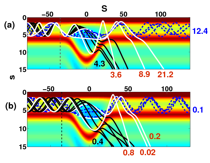
Figure 10: (color online) (a) Trajectories with different CM kinetic energies $T_{S}$ for $s_{0L}\approx 1.56$ and $\frac{t}{T}=0.22$. The numerical values presented in the diagram correspond to the values of $T_{S}$ for the different kinds of trajectories. (b) Trajectories with different phases of relative oscillation $\frac{t}{T}$ for $T_{S}=8.88$ and $s_{0L}\approx 1.56$. The numerical values presented in the diagram correspond to the values of $\frac{t}{T}$ for the different kinds of trajectories. In both cases the dissociative trajectories of type $A$ are shown with solid white lines, while those of type $B$ are represented with solid black lines. The finally bound trajectories are presented with blue dashed lines. The vertical black dashed line indicates the position $S_{hL}$ at which the hump starts (by definition).

Trajectories. As we have seen throughout this section the initially bound trajectories are divided into two different categories: those which remain finally, i.e. after scattering, bound and those which are led to dissociation. It is evident that the finally dissociated trajectories can be further classified into those that dissociate after reaching the uniform region (type $A$) and the ones that dissociate within the hump (type $B$). Since they reach the homogeneous domain (Fig. 10), the dissociated trajectories of type $A$ have more features in common with the bound ones and this is the reason why they always occur close to the transition points. States of type $B$, on the other hand are fundamentally distinct (Fig. 10) and occur only in the middle of the dissociation regions (Fig. 9 (c)). The main difference of $A$ and $B$ trajectories is imprinted in the energy transfer. Type $A$ trajectories have always final relative energy greater than the potential barrier and overall can be thought as cases where a substantial amount of energy has been transfered from the CM to the relative motion. However, the trajectories of type $B$ pass the potential barrier with their total amount of energy $E$. Since they remain in the inhomogeneous regime for some time after dissociation, a redistribution of energy between the CM and the relative motion, is still possible leading to a sequence of loss and gain of relative energy. Therefore, their final relative energy $E_{s}$ can be lower than the height of the potential barrier (Fig. 9 (c)).

Figures 10, 11 specify the above line of arguments and identify in particular the different types of trajectories. For a constant value of $s_{0L}$, sufficiently away from the potential minimum, one can induce transitions of the form:

$$\it{A}\rightarrow\it{B}\rightarrow\it{A}\rightarrow\rm{bound~{}states}\rightarrow\it{A},$$

by varying either the CM kinetic energy (increasing $T_{S}$ (Fig. 10 (a))), or the phase of the relative oscillation (decreasing $\frac{t}{T}$, Fig. 10 (b)).

Figure 11 provides us with the complementary information of how the change of the initial relative energy $E_{s}$, imprinted in $s_{0L}$, affects the evolution of the trajectories. The trajectories presented for each $s_{0L}$ have the same $T_{S}$ and different phases $\frac{t}{T}$. For $s_{0L}=s_{min}$ (Fig. 11 (a)), a case familiar from Subsec. A, the fictitious particle does not oscillate and thus the trajectories are independent of the phase. For the value of $T_{S}$ chosen here, this set of trajectories constitutes a single dissociated state of type $A$. Increasing the relative energy (decreasing $s_{0L}$), the trajectories for various phases start to separate, but still their type remains the same (Fig. 11 (b)). A further increment of $E_{s}$ (Fig. 11 (c)) has as a result the formation of dissociative states of type $B$ for certain values of phases. Finally, for $s_{0L}$ sufficiently close to the potential barrier (Fig. 11 (d)), the amplitude of the relative oscillation increases dramatically allowing for the emergence of all the three types of trajectories, including finally bound states.

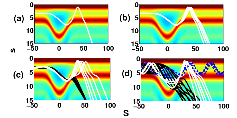
Figure 11: (color online) Trajectories for various phases of relative oscillation $\frac{t}{T}$ for $T_{S}=8.88$ and: (a) $s_{0L}=s_{min}=3.34$ (b) $s_{0L}=3.26$, (c) $s_{0L}=2.53$, (d) $s_{0L}=1.56$. Solid white lines stand for finally dissociated states of type $A$, solid black lines for type $B$, and dashed blue lines for finally bound states.

Energy transfer. Throughout this section we have come across intriguing effects originating from the coupling between the CM and the relative coordinate. The key ingredient allowing for these effects is the energy transfer between the two degrees of freedom inside the inhomogeneous region. Let us therefore point out some basic features of the energy exchange process. To do so, we consider the change of the kinetic energy of the CM $T_{S}$. The latter is zero in the uniform regime of the helix. From the equations of motion for the Hamiltonian (14) we obtain $\dot{T}_{S}=-\dot{S}\frac{\partial V}{\partial S}$, where $V=V(S,s)$. Although this relation for $\dot{T}_{S}$ refers to certain time evolving trajectories we find it instructive to analyze its contour plot for a certain value of $\dot{S}=1$.

We observe in Fig. 12 (a), that for a constant value of the CM velocity, the rate of change of $T_{S}$ is non-zero only in the inhomogeneous regime as expected. Moreover it is antisymmetric with respect to the center of the hump $S=0$, meaning that if at $(-S,s)$ the particle gains $T_{S}$, it loses at $(S,s)$. Therefore, almost symmetric trajectories $(S\rightarrow-S)$, as those for very large or very small initial CM velocity $\dot{S}_{0}$, will have finally almost zero energy transfer. However, since $T_{S}$ - moving from a positive $\dot{T}_{S}$ value to a negative one - reaches a maximum for these trajectories inside the inhomogeneity (at $S\approx 0$), the average kinetic energy of the CM motion inside the hump will be larger than that in the homogeneous regime. This in turn leads to a larger effective $\dot{S}$ within the inhomogeneity and a smaller dwell time (defined as the time interval during which the fictitious particle moves from $-S_{h}$ to $S_{h}$) than the one expected by $\dot{S}_{0}$. This effect is evident (Fig. 12 (b)) only in the case of small $\dot{S}_{0}$, where even a slight increment in the velocity affects substantially the value of the dwell time.

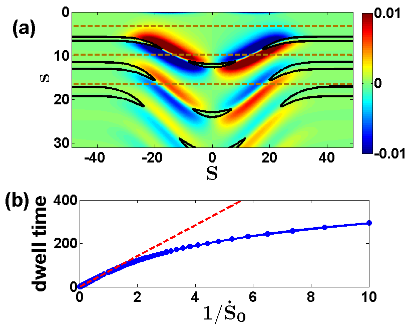
Figure 12: (color online) (a) The rate of change of the kinetic CM energy $\dot{T}_{S}$ as a function of $S,s$ for $\dot{S}=1$. The solid black lines depict the position of the maxima of the three potential barriers, while the dashed brown lines indicate the position of the minima of the three potential wells in the uniform regime (see also Fig. 3). (b) The dwell time as a function of the initial CM velocity $\dot{S}_{0}$ for the particles starting at the minimum of the first potential well with zero relative velocity (blue line with circles). For small $\dot{S}_{0}$ the deviation from a motion with constant $\dot{S}=\dot{S}_{0}$ dictated by the red dashed line, is evident.

The greatest amount of energy can be gained or lost when the fictitious particle passes deep in the potential well, close to the potential barrier since the gradient $\frac{\partial V}{\partial S}$ acquires there its largest values (Figs. 3, 12 (a)). For $\dot{S}>0$ which is always true for particles passing from the left homogeneous regime to the right one, the CM gains kinetic energy while being in the first potential well in the region $S<0$, and it loses for $S>0$. This causes highly asymmetric trajectories as some with $\dot{S}_{0}>1$ (Figs. 10, 11) overall to lose an amount of CM kinetic energy, which after reaching the uniform regime appears as a gain in the total relative energy. Trajectories that dissociate within the hump (type $B$), after crossing the top of the potential barrier for $S>0$, regain CM kinetic energy $T_{S}$ (Figs. 3, 12 (a)), but since they continue moving at lower values of the potential this does not always result in lower final values of total relative energy. Therefore, we may conclude that all the dissociative trajectories with a lowered final $E_{s}$ belong to type $B$, but not vice-versa.

Overall, it is evident that the energy transfer consists of subsequent losses and gains of $T_{S}$ and $T_{s}$ induced by the variations of the potential $V(S,s)$ inside the inhomogeneous region, leading to a final asymptotic effective gain or loss.

We explore now the structure of the underlying phase space of the scattering process and in particular of bound states in the inhomogeneity of the helix. Since the three potential wells display similar characteristics, with the first one allowing for more variations in energy since it is the deepest one, it will be the only one we consider here. For Hamiltonian systems with two degrees of freedom the standard tool for such an analysis is the Poincaré surface of section (PSOS), taking advantage of the conservation of energy. Here, we will choose $S=0~{}(P>0)$ as the intersection through the energy shell. We note that the PSOS shown below report only the bound state trajectories.

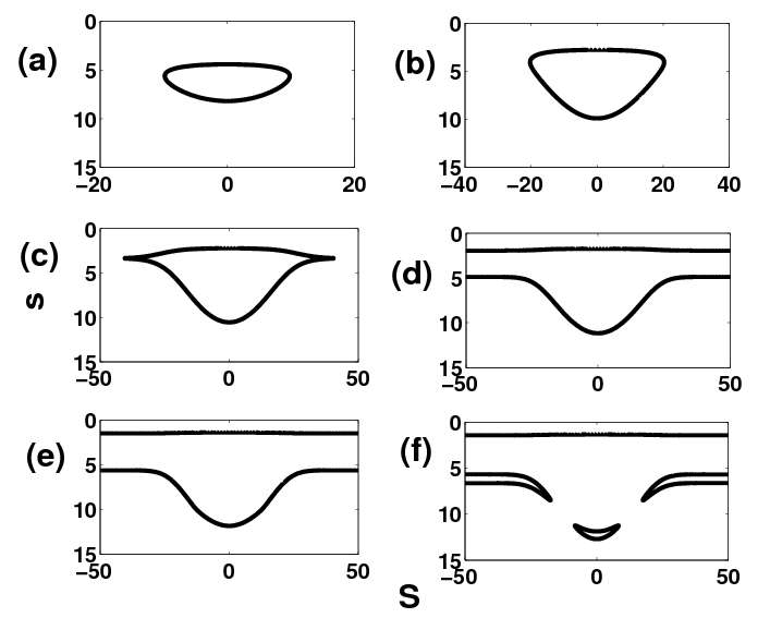
Figure 13: (color online) EPLs of the first potential well for representative total energies: (a) $E=0.28$, (b) $E=0.39$, (c) $E=0.476$, (d) $E=0.6$, (e) $E=0.744$ and (f) $E=0.76$.

Let us inspect the regions of bound and unbound motion within the inhomogeneous helix. The only part of the potential landscape $V(S,s)$ that can support bounded motion is that of the inhomogeneity, i.e. inside the hump, in the neighborhood of $S\approx 0$. Since the potential wells possess finite barriers, it is evident that for energies beyond a certain amount the fictitious particle can escape to infinity concerning either the CM $S$ or the relative coordinate $s$, leading to dissociation.

For the first potential well this fact is clearly depicted (Fig. 13) through the equipotential lines (EPLs). For $E\leq E_{c_{1}}=0.476$, with $E_{c_{1}}$ being the energy of the minimum of the first potential well in the uniform domain, the EPLs are closed both in $S$- and $s$-direction (Fig. 13 (a)-(c)) leading to exclusively bounded motion inside the hump. Figure 13 (c) presents the critical case, a fact that is reflected in the substantial elongation of the wings of the EPL. A further increment of the energy leads to EPLs extending to $\left|S\right|\rightarrow\infty$ (Figs. 13 (d)-(f)) which allows for escaping trajectories from the center of the hump to the homogeneous regime of the helix. This holds until the second critical value $E_{c_{2}}=0.744$ (Fig. 13 (e)) is reached. From then on, two additional openings are formed in the EPL inside the central region of the hump (Fig. 13 (f)) allowing also for escapes in the relative coordinate. For energies larger than the maximum value of the first potential well $V_{max}=0.81$ of course, the particles’ motion is in principle unbounded.

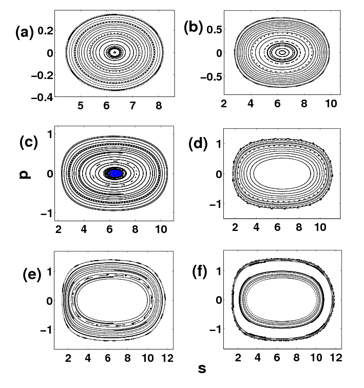
Figure 14: (color online) Poincaré surfaces of section for representative total energies: (a) $E=0.28$, (b) $E=0.39$, (c) $E=0.476$, (d) $E=0.6$, (e) $E=0.744$ and (f) $E=0.76$. The blue dots denote chaotic trajectories.

Figure 14 shows PSOS for different energies. For $E<E_{c_{1}}$ (Fig. 14 (a), (b)) we observe an elliptic island. Close to the first transition point $E=E_{c_{1}}$ (Fig. 14 (c)) it develops in its inner region, i.e. for small $p$ and $s$ close to the absolute minimum of the first potential well, a chaotic portion. A further increase of the energy leads to escaping trajectories which is evident in Fig. 14 (d) where a large part of the inner region of the surface of section (empty region) belongs to escaping trajectories $(\left|S\right|\rightarrow\infty)$ through the respective openings of the EPL (Fig. 13 (d)). As the energy approaches its second critical value $E_{c_{2}}$ (Fig. 14 (e)) the basin of escape becomes larger and finally for $E>E_{c_{2}}$ (Fig. 14 (f)), a second area of the surface of section empties, this time in the center of the region of bounded motion. This corresponds to trajectories that escape in the $s$-direction (dissociation) through the two additional openings on the lower side of the corresponding EPL (Fig. 13 (f)).

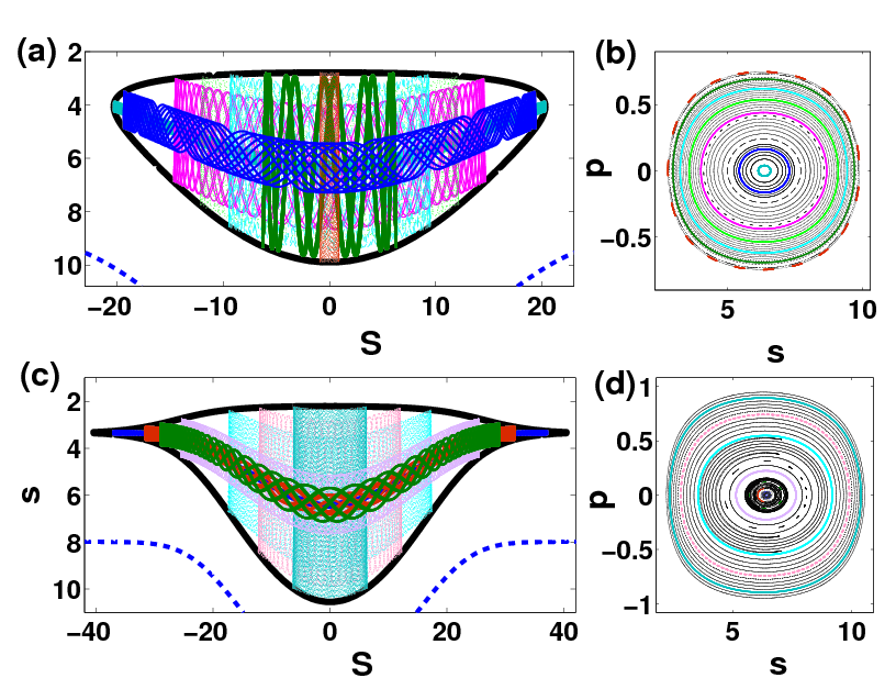
Figure 15: (color online) Selected trajectories (a),(c) and respective PSOS (b), (d) for the energies: (a),(b) $E=0.39$, (c),(d) $E=0.4761$. The color of the trajectories corresponds to their position in the PSOS. In (a),(c) the EPLs are also depicted as in Fig. 13.

Figures 15, 16 and 18 provide further details enriching the above analysis in terms of specific trajectories. First we remark that the turning points of the trajectories both in $s$- and $S$-direction, lie on the EPLs of the respective energy. Trajectories with a larger $S$ elongation and a reduced $s$-amplitude follow obviously the bending of the potential landscape and are the ones that map to the inner region of the Poincaré surface of section. As we move to the outer region of the surface of section the amplitude in $s$ increases with a respective decrease of the amplitude in the $S$-direction. For energies $E_{c_{1}}<E<E_{c_{2}}$ trajectories can escape from the left and right openings of the respective EPL (Fig. 16 (c)). In order to be bound, the trajectories should have an amplitude of the relative motion exceeding the width of the openings of the EPL (Fig. 16 (a)). This is the reason why for the PSOS the regime of bounded motion is located in the outer part, with the inner one being empty and corresponding to escaping trajectories (Fig. 16 (b)).

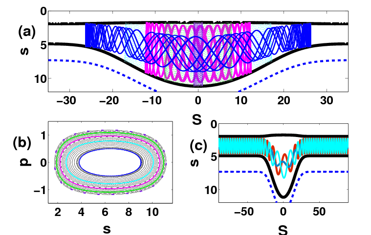
Figure 16: (color online) (a) Selected bound trajectories, (b) PSOS and (c) escaping trajectories in the CM $S$ coordinate for the energy $E=0.6$.

A more detailed nonlinear dynamical analysis would most probably reveal two unstable periodic orbits that provide the connection between the bounded and escaping motion. To explore this in detail goes however beyond the scope of the present work which has its emphasis on the main phenomena appearing in the helical dynamics investigated here for the first time.

Bridging between bound and unbound there are ”resonant” trajectories, i.e. trajectories that remain within the hump performing oscillatory CM and relative motion, for a large time interval and finally escaping to the homogeneous asymptotic region. They have typical initial conditions in the empty region of the PSOS (Fig. 16 (b)), close to the innermost bound trajectory. Such a trajectory is presented in Fig. 17. It escapes to the left opening of the potential well ($S<0$) both in forward and in backward propagation time, i.e. it is reflected at the helical hump.

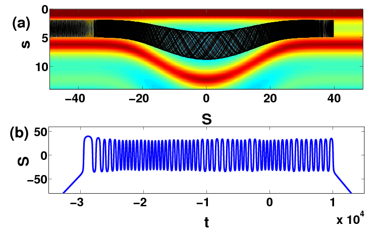
Figure 17: (color online) A resonant trajectory for $E=0.6$ and initial conditions $S=0,~{}s=5.134,~{}\dot{S}=0.549,~{}\dot{s}=-0.387$: (a) plot of the trajectory on the potential landscape, (b) time evolution of the CM coordinate $S$ of the trajectory.

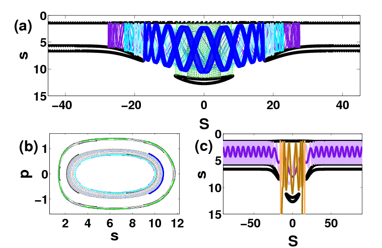
Figure 18: (color online) (a) Selected bound trajectories, (b) PSOS and (c) escaping trajectories both in the CM $S$ (bound states) and in the relative coordinate $s$ (free states) for energy $E=0.76$.

A more complex structure of the PSOS is encountered for $E_{c_{2}}<E<V_{max}$. In such a case, as we have remarked earlier, there are four openings of the EPL. Subsequently, four unstable periodic orbits exist and thus four possibilities for escape symmetric with respect to $S=0$ (Fig. 18 (c)): two in the CM coordinate direction ($S$-openings) as before and two in the relative one ($s$-openings). The escape in the $S$-direction (small $s$, large $S$, i.e. $s_{1}s_{2}>0$) both in forward and in backward propagation time, corresponds to a bound pair of particles that after scattering within the hump remains bound, a case that has been referred in the previous section as a bound state. On the contrary, escapes in $s$-direction (large $s$, small $S$) correspond to free particles that come from opposite sides of the helical trap ($s_{1}s_{2}<0$), scatter within the hump and return backwards in opposite directions. They thus account for conventional scattering of free particles and are different from the peculiar dissociative states we have observed so far.

Between the regimes of escapes, there are two distinct regions of bounded trajectories (blue and green, Fig. 18 (a)). The first of them consists of trajectories supported by the side parts of the EPL. Their relative oscillation $s$-amplitude is bounded both from below, by the width of the $S$-opening in the uniform domain, and from above by its edge width inside the inhomogeneous region. The second consists of bound states with somewhat larger relative $s$-amplitude dictated by the width of the central part of the EPL. These considerations, give rise to the two-ring structure of the PSOS (Fig. 18 (b)).

VI. SUMMARY AND OUTLOOK

We have investigated the classical scattering of Coulomb interacting particles in a helix. First, we have proven that for two particles interacting via a potential that depends exclusively on their Euclidean distance, a separation of the CM, leading to a conservation of the total momentum is provided if and only if the confining curve is a homogeneous helix. Having this result in mind, we investigated the scattering of charged particles from a local inhomogeneity of the helix. In such a system the coupling between the CM and the relative degrees of freedom induces intriguing effects. The most important of them is the dissociation of initially bound states of the two repulsively interacting charged particles through scattering. Due to the time reversal symmetry imprinted in the equations of motion, this leads to the conclusion that initially unbound charged particles can become bound when scattered, a fact counterintuitive regarding especially the repulsive character of the interaction.

The underlying mechanism for such a behaviour was found to be the effective energy transfer between the relative and the CM motion occurring due to their coupling. It has been pointed out, nevertheless, that this transfer does not take place in a single step, but it is the final result of the continuous energy redistribution in the whole time interval in which the particles remain inside the hump. For this reason, the outcome of the scattering of initially bounded charged particles in terms of finally bound and dissociated states, depends in a rather complex way on the initial conditions. The dissociation regimes depending on these condition have been identified and analyzed in detail. The most important parameter is shown to be the value of the initial kinetic energy of the CM $T_{S}$. In most cases for very small or very large values of $T_{S}$ the particles remain bound after the scattering, with dissociation occurring only in the intermediate regime. This is attributed to the little amount of energy available for transfer and to the small dwell time in the hump that prevents a strong coupling of the relative and CM degrees of freedom respectively.

Our analysis has been completed with an exploration of the phase space structure of the deepest potential well that can support bound states. Regimes of bound regular motion inside the hump, as well as regimes of escapes were identified by varying the total energy. This exploration provided us with bound states localized inside the hump, as well as with ”resonant trajectories“.

Further studies could be dedicated to a more detailed investigation of the phase space searching for stable and unstable periodic orbits and their asymptotic curves, a fact that would allow a rigorous and quantitative analysis of the escape procedure. A promising direction is the study of many-body systems which are expected to exhibit an intriguing dynamics as well as leading to exceptional transition phenomena.

Proposition: The condition:

$$\partial_{s_{1}}R(s_{1},s_{2})+\partial_{s_{2}}R(s_{1},s_{2})=0,~{}\forall s_{1},s_{2}\in\mathbb{R},$$ (17)

where $R(s_{1},s_{2})=\left|\mathbf{r}(s_{1})-\mathbf{r}(s_{2})\right|$ holds for a smooth, regular curve $\mathbf{r}(s)$ in arc length parametrization if and only if the curve is a homogeneous helix (including the degenerate cases of a circle or a straight line).

Proof: ”$\Leftarrow$“: By the discussion in section II, condition (17) is equivalent to separability of CM and relative motion, which has been demonstrated to hold for a homogeneous helix (see discussion in the main text).

”$\Rightarrow$“: Assume that condition (17) holds. The outline of the proof is as follows. We show that by virtue of Eq. (17), for each $x\in\mathbb{R}$ the map

$$F_{x}:\mathcal{W}\mapsto\mathcal{W},~{}F_{x}(\mathbf{r}(s))=\mathbf{r}(s+x).$$ (18)

is an isometry (i.e. it preserves distances) on the submanifold $\mathcal{W}\subseteq\mathbb{R}^{3}$, which is defined as the image of the curve $\mathbf{r}$. We extend this family of isometries to a family of isometries $\left\{\Gamma_{x}\right\}_{x\in\mathbb{R}}$ from all of $\mathbb{R}^{3}$ into itself, with the property that the restriction $\Gamma_{x}\big{|}_{\mathcal{W}}=F_{x}$. The isometries of $\mathbb{R}^{3}$ form the group of Euclidean moves $E(3)$. Since the $\Gamma_{x}$ are continuously deformed to the identity map for $x\rightarrow 0$, they belong to the identity component of $E(3)$, i.e. to $SE(3)$. Thus by the classification theorem for Euclidean moves Tarrida each $\Gamma_{x}$ is a screw operation or a degenerate case thereof, i.e. a pure rotation or translation. Furthermore, not all $\Gamma_{x}$ can be the identity on $\mathbb{R}^{3}$, since then the curve $\mathbf{r}$ would have the property $\mathbf{r}(s+x)=\mathbf{r}(s)$ for all $x$ and would degenerate to a point. Thus, there is at least one non-trivial screw operation $\Gamma_{x}$ that maps the curve $\mathcal{W}$ to itself, so $\mathcal{W}$, the image of $\mathbf{r}(s)$, must be a (homogeneous) helix, which proves the proposition.

We now proceed to the detailed proof and first show that, given Eq. (17), the map $F_{x}$ as defined in (18) is an isometry on $\mathcal{W}$. First we prove that there is a function $\chi$ such that $R(s_{1},s_{2})=\chi(s_{1}-s_{2})$. To see this, introduce new variables $\xi_{-}:=s_{1}-s_{2},~{}\xi_{+}:=s_{1}+s_{2}$ and a function $\chi$ with the property $\chi(\xi_{+},\xi_{-})=R(s_{1},s_{2})$. Then condition (17) yields $\partial\chi/\partial\xi_{+}=0$, leading to $\chi(\xi_{+},\xi_{-})=\chi(\xi_{-})$ or

$$R(s_{1},s_{2})=\chi(s_{1}-s_{2}).$$

This, in turn, immediately implies $R(s_{1},s_{2})=R(s_{1}+x,s_{2}+x)$, or

$$\left|\mathbf{r}(s_{1})-\mathbf{r}(s_{2})\right|=\left|\mathbf{r}(s_{1}+x)-\mathbf{r}(s_{2}+x)\right|$$

for all $x,s_{1},s_{2}\in\mathbb{R}$, showing that indeed $F_{x}$ as defined above is an isometry on $\mathcal{W}$.

We now assume without loss of generality that $\mathbf{0}\in\mathcal{W}$ and proceed to show that for all $x$ the map

$$\tilde{F}_{x}:\mathcal{W}\mapsto\mathbb{R}^{3},~{}\tilde{F}_{x}(\mathbf{r}):=F_{x}(\mathbf{r})-F_{x}(\mathbf{0})$$

has the following properties:
(i) $\left|\tilde{F}_{x}(\mathbf{r})\right|=\left|\mathbf{r}\right|\,\,\,\,\,\,\forall\mathbf{r}\in\mathcal{W}$.
(ii) $\sigma\left(\tilde{F}_{x}(\mathbf{r}_{1}),\tilde{F}_{x}(\mathbf{r}_{2})\right)=\sigma\left(\mathbf{r}_{1},\mathbf{r}_{2}\right)\,\,\,\,\,\forall\mathbf{r}_{1},\mathbf{r}_{2}\in\mathcal{W}$ .
(iii) $\tilde{F}\left(\alpha_{1}\mathbf{r}_{1}+\alpha_{2}\mathbf{r}_{2}\right)=\alpha_{1}\tilde{F}_{x}\left(\mathbf{r}_{1}\right)+\alpha_{2}\tilde{F}_{x}\left(\mathbf{r}_{2}\right)$
………..$\forall\mathbf{r}_{1},\mathbf{r}_{2}\in\mathcal{W},\alpha_{1},\alpha_{2}\in\mathbb{R}\text{ s.t. }\alpha_{1}\mathbf{r}_{1}+\alpha_{2}\mathbf{r}_{2}\in\mathcal{W}$.
Here $\sigma$ denotes the Euclidean scalar product. (i) immediately follows from $F_{x}$ being an isometry on $\mathcal{W}$. (ii) follows from (i) and $F_{x}$ being an isometry, since $\forall\mathbf{r}_{1},\mathbf{r}_{2}\in\mathcal{W}$:

$$2\sigma(\tilde{F}_{x}(\mathbf{r}_{1}),\tilde{F}_{x}(\mathbf{r}_{2}))$$

$$= \left|\tilde{F}_{x}(\mathbf{r}_{1})\right|^{2}+\left|\tilde{F}_{x}(\mathbf{r}_{2})\right|^{2}-\left|\tilde{F}_{x}(\mathbf{r}_{1})-\tilde{F}_{x}(\mathbf{r}_{2})\right|^{2}$$

$$= \left|\mathbf{r}_{1}\right|^{2}+\left|\mathbf{r}_{2}\right|^{2}-\left|\mathbf{r}_{1}-\mathbf{r}_{2}\right|^{2}=2\sigma(\mathbf{r}_{1},\mathbf{r}_{2}).$$

Finally, using (i) and (ii) it is easily shown that

$$\left|\tilde{F}_{x}(\alpha_{1}\mathbf{r}_{1}+\alpha_{2}\mathbf{r}_{2})-\alpha_{1}\tilde{F}_{x}(\mathbf{r}_{1})-\alpha_{2}\tilde{F}_{x}(\mathbf{r}_{2})\right|^{2}$$

$$=\left|(\alpha_{1}\mathbf{r}_{1}+\alpha_{2}\mathbf{r}_{2})-\alpha_{1}\mathbf{r}_{1}-\alpha_{2}\mathbf{r}_{2}\right|^{2}=0,$$

which proves (iii).

Now we are in the position to construct the extended isometries $\Gamma_{x}$. Let us first assume that the curve $\mathbf{r}$ does not entirely lie in a plane. Then we can form a basis of $\mathbb{R}^{3}$ with three linearly independent vectors $\mathbf{w}_{i}\in\mathcal{W}$. Hence for each $\mathbf{x}\in\mathbb{R}^{3}$ there exists a unique expansion $\mathbf{x}=\sum_{i=1}^{3}\alpha_{i}\mathbf{w}_{i},~{}\alpha_{i}\in\mathbb{R}$. For any such $\mathbf{x}$ we define

$$\Gamma_{x}(\mathbf{x}):=F_{x}(\mathbf{0})+\sum_{i=1}^{3}\alpha_{i}\tilde{F}_{x}(\mathbf{w}_{i}).$$

Evidently, for the special case of $\mathbf{r}=\sum_{i=1}^{3}\gamma_{i}\mathbf{w}_{i}\in\mathcal{W}$:

$$\Gamma_{x}(\mathbf{r}) = F_{x}(\mathbf{0})+\sum_{i=1}^{3}\gamma_{i}\tilde{F}_{x}(\mathbf{w}_{i})=F_{x}(\mathbf{0})+\tilde{F}_{x}\left(\sum_{i=1}^{3}\gamma_{i}\mathbf{w}_{i}\right)$$

$$= F_{x}(\mathbf{0})+\tilde{F}_{x}(\mathbf{r})=F_{x}(\mathbf{r}),$$

due to property (iii) of $\tilde{F}_{x}$, such that indeed the restriction $\Gamma_{x}\rvert_{\mathcal{W}}=F_{x}$. Now, using property (ii) of $\tilde{F}_{x}$, it is straightforward to show that for any $\mathbf{x}$ and $\mathbf{y}=\sum_{i=1}^{3}\beta_{i}\mathbf{w}_{i}\in\mathbb{R}^{3}$:

$$\left|\Gamma_{x}(\mathbf{x})-\Gamma_{x}(\mathbf{y})\right|^{2}=\left|\sum_{i=1}^{3}(\alpha_{i}-\beta_{i})\tilde{F}_{x}(\mathbf{w}_{i})\right|^{2}$$

$$= \left|\sum_{i=1}^{3}(\alpha_{i}-\beta_{i})\mathbf{w}_{i}\right|^{2}=\left|\mathbf{x}-\mathbf{y}\right|^{2}$$

which proves that $\Gamma_{x}$ is an isometry of $\mathbb{R}^{3}$.

Finally, we address the special case of a planar curve. Then either $\mathcal{W}$ is a straight line, in which case there is nothing to prove, since this is a degenerate case of a helix. Otherwise, we pick two linearly independent vectors $\mathbf{w}_{i}\in\mathcal{W}$ and a third vector $\mathbf{k}_{3}$ perpendicular to $\mathbf{w}_{1},\mathbf{w}_{2}$. Since $F_{x}$ maps $\mathcal{W}$ to itself it is clear that $\sigma(\tilde{F}_{x}(\mathbf{w}_{i}),\mathbf{k}_{3})=0$ as well. For any vector $\mathbf{x}\in\mathbb{R}^{3}$ a representation $\mathbf{x}=\alpha_{1}\mathbf{w}_{1}+\alpha_{2}\mathbf{w}_{2}+\alpha_{3}\mathbf{k}_{3}$ is possible and we define:

$$\Gamma_{x}(\mathbf{x})=F_{x}(\mathbf{0})+\alpha_{1}\tilde{F}_{x}(\mathbf{w}_{1})+\alpha_{2}\tilde{F}_{x}(\mathbf{w}_{2})+\alpha_{3}\mathbf{k}_{3},$$

which for $\mathbf{x}\in\mathcal{W}$ (implying $\alpha_{3}=0$) using (iii) again leads to $\Gamma_{x}\rvert_{\mathcal{W}}=F_{x}$. Furthermore, using the orthogonality of $\mathbf{k}_{3}$ to $\mathbf{w}_{i},\tilde{F}_{x}(\mathbf{w}_{i})$ as well as (ii), it follows for any $\mathbf{y}=\sum_{i=1}^{2}\beta_{i}\mathbf{w}_{i}+\beta_{3}\mathbf{k}_{3}$ that:

$$\left|\Gamma_{x}(\mathbf{x})-\Gamma_{x}(\mathbf{y})\right|^{2}=\left|\sum_{i=1}^{2}(\alpha_{i}-\beta_{i})\tilde{F}_{x}(\mathbf{w}_{i})+(\alpha_{3}-\beta_{3})\mathbf{k}_{3}\right|^{2}$$

$$= \left|\sum_{i=1}^{2}(\alpha_{i}-\beta_{i})\mathbf{w}_{i}+(\alpha_{3}-\beta_{3})\mathbf{k}_{3}\right|^{2}=\left|\mathbf{x}-\mathbf{y}\right|^{2}.$$

Therefore for this case, too, one can construct an isometry $\Gamma_{x}$ of $\mathbb{R}^{3}$ which extends $F_{x}$. Evidently, in both cases tuning $x\rightarrow 0$ one can continuously transform the $\Gamma_{x}$ to $\Gamma_{x=0}=\text{id}_{\mathbb{R}^{3}}$, such that all $\Gamma_{x}$ lie in $SE(3)$.

ACKNOWLEDGEMENTS

We thank M. Jüngling for many helpful discussions and his support concerning the theoretical conceptual aspects of this work. A. Z. thanks the International Max Planck Research School for Ultrafast Imaging and Structural Dynamics for a PhD scholarship. J. S. and S. K. gratefully acknowledge funding by the Studienstiftung des deutschen Volkes.

References

- (1) H. Totsuji and J.-L. Barrat, Phys. Rev. Lett. 60, 2484 (1988).
- (2) G. Vernizzi, K. L. Kohlstedt and M. Olvera de la Cruz, Soft Matter 5, 736 (2009).
- (3) G. E. Desobry and P. K. Kabir, Am. J. Phys. 41, 1350 (1973).
- (4) F. Dufey, Chem. Phys. 330, 326 (2006).
- (5) R. C. T. da Costa, Phys. Rev. A 23, 1982 (1981).
- (6) P. Exner and M. Fraas, Phys. Lett. A 369, 393 (2007).
- (7) J. Goldstone and R. L. Jaffe, Phys. Rev. B 45, 14100 (1992).
- (8) O. V. Kibis et al., Electromagnetics 25, 425 (2005).
- (9) K. T. Law and D. E. Feldman, Phys. Rev. Lett. 101, 096401 (2008).
- (10) V. Y. Prinz et al., Physica E 6, 828 (2000).
- (11) O. G. Schmidt and K. Eberl, Nature 410, 168 (2001).
- (12) M. Bhattacharya, Opt. Comm. 279, 219 (2007).
- (13) A. Okulov, Phys. Lett. A 376, 650 (2012).
- (14) I. Ricardez-Vargas and K. Volke-Sepúlveda, J. Opt. Soc. Am. B 27, 948 (2010).
- (15) E. Vetsch et al., Phys. Rev. Lett. 104, 203603 (2010).
- (16) E. Vetsch et al., IEEE J. Quant. Electr. 18, 1763 (2012).
- (17) D. Reitz and A. Rauschenbeutel, Opt. Comm. 285, 4705 (2012).
- (18) W. Paul, Rev. Mod. Phys. 62, 531 (1990).
- (19) Ch. Schneider, M. Enderlein, T. Huber and T. Schaetz, Nature Photonics 4, 772 (2010).
- (20) P. Schmelcher, Europhys. Lett. 95, 50005 (2011).
- (21) The property of having either a closed or infinitely extended curve can be formalised in terms of the arc length: For any arc length , must be well defined, i.e. a point of the space curve under consideration.
- (22) A. R. Tarrida, Affine Maps, Euclidean Motions and Quadrics, Springer-Verlag, (2011).