Qualitative analysis of Kantowski-Sachs metric in a generic class of $f(R)$ models

Abstract

In this paper we investigate, from the dynamical systems perspective, the evolution of a Kantowski-Sachs metric in a generic class of $f(R)$ models. We present conditions (i. e., differentiability conditions, existence of minima, monotony intervals, etc.) for a free input function related to the $f(R)$, that guarantee the asymptotic stability of well-motivated physical solutions, specially, self-accelerated solutions, allowing to describe both inflationary- and late-time acceleration stages of the cosmic evolution. We discuss which $f(R)$ theories allows for a cosmic evolution with an acceptable matter era, in correspondence to the modern cosmological paradigm. We find a very rich behavior, and amongst others the universe can result in isotropized solutions with observables in agreement with observations, such as de Sitter, quintessence-like, or phantom solutions. Additionally, we find that a cosmological bounce and turnaround are realized in a part of the parameter-space as a consequence of the metric choice.

1 Introduction

Several astrophysical and cosmological measurements, including the recent WMAP nine year release, and the Planck measurements, suggest that the observable universe is homogeneous and isotropic at the large scale and that it is currently experiencing an accelerated expansion phase [2, 3, 1, 4, 5, 6]. The explanation of the isotropy and homogeneity of the universe and the flatness problem lead to the construction of the inflationary paradigm [7, 8, 9, 10] . Usually in the inflationary scenarios the authors start with a homogeneous and isotropic Friedmann-Robertson-Walker metric (FRW) and then are examined the evolution of the cosmological perturbations. However, the more strong way to proceed is to put from the beginning an arbitrary metric and then examine if the metric tends asymptotically to the flat FRW geometry . This is a very difficult program even using a numerical approach, see for example the references [14, 15, 16]. Thus, several authors investigated the special case of homogeneous but anisotropic Bianchi [19, 17, 18] (see [20] and references therein) and the Kantowski-Sachs metrics [21, 22, 48, 23, 24, 25, 26, 36, 27, 37, 38, 28, 29, 30, 39, 40, 31, 41, 42, 43, 32, 44, 45, 33, 46, 35, 34, 47]. The simplest well-studied but still very interesting Bianchi geometries are the Bianchi I [63, 49, 50, 51, 23, 24, 52, 53, 54, 55, 57, 56, 58, 59, 60, 61, 62, 47] and Bianchi III [64, 23, 65, 66, 47], since other Bianchi models (for instance the Bianchi IX one), although more realistic, they are much more complicated. These geometries have been examined analytically, exploring their rich behavior, for different matter content of the universe and for different cosmological scenarios (e.g., [17, 18, 49, 50, 23, 24, 52, 53, 68, 54, 55, 57, 56, 58, 59, 60, 61, 62, 64, 65, 66, 25, 26, 67, 27, 28, 29, 30, 31, 32, 33, 34, 35, 69, 70, 71, 72, 73, 74, 76, 75, 77, 78, 47]).

On the other hand, to explain the acceleration of the expansion one choice is to introduce the concept of dark energy (see [79, 80, 81] and references therein), which could be the simple cosmological constant, a quintessence scalar field [82, 83, 84, 85], a phantom field [86, 87, 88, 89, 90], or the quintom scenario [91, 92, 93, 96, 97, 94, 95, 98]. The second one is to consider Extended Gravity models, specially the $f(R)$- models (see [99, 100, 101, 102, 105, 103, 106, 104] and references therein), as alternatives to Dark Energy. Other modified (extended) gravitational scenarios that have gained much interests due to their cosmological features are the extended nonlinear massive gravity scenario [107, 108, 109, 110], and the Teleparalell Dark Energy model [111, 112, 113]. However, we follow the mainstream and investigate $f(R)$ models.

$f(R)$-models have been investigated widely in the literature. In particular, Bianchi I models in the context of quadratic and $f(R)$ cosmology were first investigated in [63], where the authors showed that anisotropic part of the spacetime metric can be integrated explicitly. In the reference [114] was done a phase-space analysis of a gravitational theory involving all allowed quadratic curvature invariants to appear in the Lagrangian assuming for the geometry the Bianchi type I and type II models, which incorporate both shear and 3-curvature anisotropies. The inclusion of quadratic terms provides a new mechanism for constraining the initial singularity to be isotropic. Additionally, there was given the conditions under which the de Sitter solution is stable, and for certain values of the parameters there is a possible late-time phantom-like behavior. Furthermore, there exist vacuum solutions with positive cosmological constant which do not approach de Sitter at late times, instead, they inflate anisotropically [114]. In the references [115, 116, 117] were investigated the oscillations of the $f(R)$ dark energy around the phantom divide line, $w_{DE}=-1$. The analytical condition for the existence of this effect was derived in [116]. In [117] was investigated the phantom divide crossing for modified gravity both during the matter era and also in the de Sitter epoch. The unification of the inflation and of the cosmic acceleration in the context of modified gravity theories was investigated for example in [118]. However, this model is not viable due the violation of the stability conditions. The first viable cosmological model of this type was first constructed in [119], requiring a more complicated $f(R)$ function. In [120] was developed a general scheme for modified $f(R)$ gravity reconstruction from any realistic FRW cosmology; another reconstruction method using cosmic parameters instead of the time law for the scale factor, was presented and discussed in [121]. Finally, in the reference [122] is described the cosmological evolution predicted by three distinct $f(R)$ theories, with emphasis on the evolution of linear perturbations. Regarding to linear perturbations in $f(R)$ viable cosmological models, the more important effect, which is the anomalous growth of density perturbations was, prior to reference [122], considered in [123, 124].

In this paper we investigate from the dynamical systems perspective the viability of cosmological models based on Kantowski-Sachs metrics for a generic class of $f(R)$, allowing for a cosmic evolution with an acceptable matter era, in correspondence to the modern cosmological paradigm. We present sufficient conditions (i.e., differentiability conditions, existence of minima, monotony intervals, an other mathematical properties for a free input function) for the asymptotic stability of well-motivated physical solutions, specially, self-accelerated solutions, allowing to describe both inflationary and late-time acceleration. The procedure used for the examination of arbitrary $f(R)$ theories was first introduced in the reference [125] and the purpose of the present investigation is to improve it and extend it to the anisotropic $f(R)$ scenario. Particularly, in [125] the authors demonstrated that the cosmological behavior of the flat Friedmann- Robertson-Walker $f(R)$ models can be understood, from a geometric perspective, by analyzing the properties of a curve $m(r)$ in the plane $(r,m)$, where

$$m=\frac{Rf^{\prime\prime}(R)}{f^{\prime}(R)}=\frac{d\ln{f^{\prime}(R)}}{d\ln R}$$

and

$$r=-\frac{Rf^{\prime}(R)}{f(R)}=-\frac{d\ln{f(R)}}{d\ln R}.$$

However, as discussed in [126], the approach in [125] is incomplete, in the sense that the authors consider only the condition $1+r+m(r)=0$ to define the singular values of $r$ and they omit some important solutions satisfying $r=0$ and/or $\frac{\dot{R}}{HR}=0.$ This leads to changes concerning the dynamics, and to some inconsistent results when comparing with [126]. It is worthy to mention that using our approach it is possible to overcome the previously commented difficulties -remarked in Ref. [126]- about the approach of Ref. [125] (see details at the end of section 3.2). However, since the analysis in references [125] and [126], is qualitative, an accurate numerical analysis is required. This numerical elaboration was done in [127] for the case of $R^{n}$-gravity, where the authors considered the whole mixture of matter components of the Universe, including radiation, and without any identification with a scalar tensor theory in any frame. There was shown numerically that for the homogeneous and isotropic $R^{n}$ model, including the case $n=2$, an adequate matter dominated era followed by a satisfactory accelerated expansion is very unlikely or impossible to happen. Thus, this model seems to be in disagreement with what is required to be the features of the current Universe as noticed in [125]. Regarding the investigations of the $f(R)\propto R^{n},$ it is worthy to note that, in the isotropic vacuum case, this model can be integrated analytically, see [128].

In the reference [129] are investigated, from the dynamical systems viewpoint and by means of the method developed in [125], the so-called $f(R,T)$ theory, where $T$ is the trace of the energy-momentum tensor. This theory was first proposed in [130]. In [129] was investigated the flat Friedmann- Robertson- Walker (FRW) background metric. Specially, for the class $f(R,T)=g(R)+h(T),h\neq 0,$ the only form that respects the conservation equations is $f(R,T)=g(R)+c_{1}\sqrt{-T}+c_{2}$ where $c_{i},i=1,2$ do not depend on T, but possibly depends on $R.$ We recover the results in [129] for this particular $f(R,T)$ choice in the isotropic regime. However, our results are more general since we consider also anisotropy.

In the reference [131] are investigated FRW metric on the framework of $f(R)=R+\alpha R^{n}$ gravity using the same approach as in [126]. Bianchi I universes in $R^{n}$ cosmologies with torsion have been investigated in [132]. In the reference [133] the authors examine the asymptotic properties of a universe based in a Scalar-tensor theory (and then related through conformal transformation to $f(R)$-theories). They consider an FRW metric and a scalar field coupled to matter, also it is included radiation. The authors prove that critical points associated to the de Sitter solution are asymptotically stable, and also generalize the results in [134]. The analytical results in [133] are illustrated for the important modified gravity models $f(R)=R+\alpha R^{2}$ (quadratic gravity) and $f(R)=R^{n}$. For quadratic gravity, it is proved, using the explicit calculation of the center manifold of the critical point associated to the de Sitter solution (with unbounded scalar field) is locally asymptotically unstable (saddle point). In this paper we extent these results to the Kantowski-Sachs metrics. Finally, in the reference [34] were investigated $R^{n}$-gravity models for anisotropic Kantowski-Sachs metric. There were presented conditions for obtaining late-time acceleration, additionally, in the range $2<n<3$, it is obtained phantom behavior. Besides, isotropization is achieved irrespectively the initial degree of anisotropy. Additionally, it is possible to obtain late-time contracting and cyclic solutions with high probability. In this paper we extent the results in [125, 133, 34] to the Kantowski-Sachs metric. Particularly, we formalize and extent the geometric procedure discussed in [125] in such way that the problems cited in [126] do not arise, and apply the procedure to “generic” $f(R)$ models for the case of a Kantowski-Sachs metric. By “generic” we refer to starting with a unspecified $f(R)$, and then deduce mathematical properties (differentiability, existence of minima, monotony intervals, etc) for the free input functions in order to obtain cosmological solutions compatible with the modern cosmological paradigm. We extent the results obtained in the reference [133] related to the stability analysis for the de Sitter solution (with unbounded scalar field) for the homogeneous but anisotropic Kantowski-Sachs metric and we extent to generic $f(R)$ models of the results in [34] that were obtained for $R^{n}$-cosmologies. Our results are also in agreement with the related ones in [129].

The paper is organized as follows. In section 2 we construct the cosmological scenario of anisotropic $f(R)$-gravity, presenting the kinematic and dynamical variables specifying the equations for the Kantowski-Sachs metric. Having extracted the cosmological equations in section 3 we perform a systematic phase-space and stability analysis of the system. It is presented a general method for the qualitative analysis of $f(R)$-gravity without considering an explicit form for the function $f(R)$. Instead we leave the function $f(R)$ as a free function and use a parametrization that allows for the treatment of arbitrary (unspecified) $f(R)$ anzatzes. In section 4 we present a formalism for the physical description of the solutions and it is discussed the connection with the cosmological observables. In the section 5 we analyze the physical implications of the obtained results, and we discuss the cosmological behaviors of a generic $f(R)$ in a universe with a Kantowski-Sachs geometry. In section 6 are illustrated our analytical results for a number of $f(R)$-theories. Our main purpose is to illustrate the possibility to realize the matter era followed by a late-time acceleration phase. Additionally it is discussed the possibility of a bounce or a turnaround. Finally, our results are summarized in section 7.

2 The cosmological model

In this section we consider an $f(R)$-gravity theory given in the metric approach with action [102, 105, 106]

$$S_{met}=\int_{V}d^{4}x\sqrt{-g}\left[f(R)-2\Lambda+L_{m}\right],$$ (2.1)

where $L_{m}$ is the matter Lagrangian. Additionally, we use the metric signature ($-1,1,1,1$). Greek indexes run from $0$ to $3$, and we impose the standard units in which $\kappa^{2}\equiv 8\pi G=c=1$. Also, in the following, and without loss of generality, we set the usual cosmological constant $\Lambda=0.$ Furthermore, $f(R)$ is a function of the Ricci scalar $R$, that satisfies the following very general conditions [119]:

1. Existence of a stable Newtonian limit for all values of $R$ where the Newtonian gravity accurately describes the observed inhomogeneities and compact objects in the Universe, i.e., for $R\gg R_{0}\equiv R(t_{0})$, where $t_{0}$ is the present moment and $R_{0}$ is the present FRW background value, and up to curvatures in the center of neutron stars:

   $$|f(R)-R|\ll R,\;|f^{\prime}(R)-1|\ll 1,\;Rf^{\prime\prime}(R)\ll 1,$$ (2.2)

   for $R\gg R_{0}$. The last of the conditions (2.2) implies that its Compton wavelength is much less than the radius of curvature of the background space-time. Additionally, the conditions (2.2) guarantee that non-GR corrections to a space-time metric remain small [119].

2. Classical and quantum stability:

   $$f^{\prime}(R)>0,f^{\prime\prime}(R)>0.$$ (2.3)

   The first condition implies that gravity is attractive and the graviton is not ghost. Its violation in an FRW background would imply the formation of a strong space-like anisotropic curvature singularity with power-law behavior of the metric coefficients [135, 63]. This singularity prevents a transition to the region where the effective gravitational constant in negative in a generic, non-degenerate solution. Additionally, note that at the Newtonian regime, the effective scalaron mass squared is $M_{s}^{2}(R)=1/(3F^{\prime\prime}(R))$. Thus, the second condition in (2.3) implies that the scalaron is not a tachyon, i.e., the scalaron has a finite rest-mass $M_{s}=(3f^{\prime\prime}(R))^{-\frac{1}{2}}.$ If $f^{\prime\prime}(R)$ becomes zero for a finite $R=R_{c}$, then a weak (sudden) curvature singularity forms generically [119].

3. In the absence of matter, exact de Sitter solutions are associated to positive real roots of the functional equation

   $$Rf^{\prime}(R)-2f(R)=0.$$ (2.4)

   It is well-known that these kind of solutions (and nearby solutions) are very important for the description of early inflationary epoch and the late-time acceleration phase. For the asymptotic future stability of these solutions near de Sitter ones it is required that

   $$f^{\prime}(R_{1})/f^{\prime\prime}(R_{1})>R_{1},$$

   where $R_{1}$ satisfies (2.4) [136]. Specific functional forms satisfying all this conditions have been proposed, e.g., in the references [123, 137, 124].

4. Finally, we have additionally considered the condition $Rf^{\prime}(R)-f(R)\geq 0$ to get a non-negative scalaron potential.

The fourth-order equations obtained by varying action (2.1) with respect to the metric are:

$$f^{\prime}(R)R_{\alpha\beta}-\frac{f(R)}{2}g_{\alpha\beta}-\nabla_{\alpha}\nabla_{\beta}f^{\prime}(R)+g_{\alpha\beta}\Box f^{\prime}(R)=T_{\alpha\beta},$$ (2.5)

where the prime denotes differentiation with respect to $R$. In this expression $T_{\alpha\beta}$ denotes the matter energy-momentum tensor, which is assumed to correspond to a perfect fluid with energy density $\rho_{m}$ and pressure $p_{m}$, and their ratio gives the matter equation-of-state parameter

$$w=\frac{p_{m}}{\rho_{m}}.$$ (2.6)

$\nabla_{\alpha}$ is the covariant derivative associated with the Levi-Civita connection of the metric and $\Box\equiv\nabla^{\beta}\nabla_{\beta}$. Taking the trace of equation (2.5) we obtain “trace-equation”

$$f^{\prime}(R)R+3\Box f^{\prime}(R)-2f(R)=T,$$ (2.7)

where $T=T^{\alpha}_{\alpha}$ is the trace of the energy-momentum tensor of ordinary matter.

Our main objective is to investigate anisotropic cosmologies. Let us assume, as usual, an anisotropic metric of form [138]:

$$ds^{2}=-N(t)^{2}dt^{2}+[e^{1}_{1}(t)]^{-2}dr^{2}+[e^{2}_{2}(t)]^{-2}[d\theta^{2}+S(\theta)^{2}d\varphi^{2}],$$ (2.8)

where $N(t)$ is the lapse function, that we will set $N=1$, $e^{1}_{1}(t)$ and $e^{2}_{2}(t)$ are the expansion scale factors, which in principle can evolve differently.

Notice that the metric (2.8) can describe three geometric families, that is:

$$S(\theta)=\left\{\begin{array}[]{lll}\theta&\textrm{ for $k=0$}&\textrm{(Bianchi I models),}\\ \sinh\theta&\textrm{for $k=-1$}&\textrm{(Bianchi III models),}\\ \sin\theta&\textrm{for $k=1$}&\textrm{(Kantowski-Sachs (KS) models),}\end{array}\right.$$

where $k$ is the spatial curvature parameter.

From the expansion scale factors are defined the kinematic variables

$$H = -\frac{1}{3}\frac{d}{dt}{\ln\left[\;e^{1}_{1}\;(e^{2}_{2})^{2}\right]},$$ (2.9a)

$$\sigma = \frac{1}{3}\frac{d}{dt}{\ln\left[e^{1}_{1}\;(e^{2}_{2})^{-1}\right]}.$$ (2.9b)

Furthermore, ${}^{2}\!K=(e^{2}_{2})^{2}$ is the Gauss curvature of the 3-spheres [139] and their evolution equation is given by [140]

$$\dot{{}^{2}\!K} = -2(\sigma+H)\;({}^{2}\!K).$$ (2.10)

Additionally, the evolution equation for $e^{1}_{1}$ reads (see equation (42) in section 4.1 in [140])

$$\dot{e}^{1}_{1}=\left(-H+2\sigma\right){e}^{1}_{1}.$$ (2.11)

From the trace equation (2.7) for the Kantowski-Sachs geometry ($k=1$) and assuming the matter content described as a perfect fluid we obtain:

$$-3\frac{d^{2}}{dt^{2}}f^{\prime}(R)-9H\frac{d}{dt}f^{\prime}(R)+f^{\prime}(R)R-2f(R)=-\rho_{m}+3p_{m}.$$ (2.12)

The Ricci scalar is written as

$$R=12H^{2}+6\sigma^{2}+6\dot{H}+2\;{}^{2}\!K.$$ (2.13)

Now, it is straightforward to write the equation (2.5) as [141] :

$$AG_{\alpha\beta}=T_{\alpha\beta}+T^{DE}_{\alpha\beta},$$ (2.14a)

$$T^{DE}_{\alpha\beta}=(A-f^{\prime}(R))R_{\alpha\beta}+\frac{1}{2}g_{\alpha\beta}(f(R)-AR)+\left(\nabla_{\alpha}\nabla_{\beta}-g_{\alpha\beta}\Box\right)f^{\prime}(R),$$ (2.14b)

where A is some constant. In order to reproduce the standard matter era ($3H^{2}\simeq\rho_{m}$) for $z\gg 1$, we can choose $A=1$. An alternative possible choice is $A=F_{0}$, where $F_{0}$ is the present value of $f^{\prime}(R)$. This choice may be suitable if the deviation of $F_{0}$ from 1 is small (as in scalar-tensor theory with a nearly massless scalar field [86, 145]).

Substituting the Kantowski-Sachs metric into the equations (2.14a) with the definition for $T^{DE}_{\alpha\beta}$ given by (2.14b), and after some algebraic manipulations, we obtain

$$A\left(3H^{2}-3\sigma^{2}+{}^{2}\!K\right) = \rho_{m}+\rho_{DE},$$ (2.15a)

$$A\left(-3(\sigma+H)^{2}-2\dot{\sigma}-2\dot{H}-{}^{2}\!K\right) = p_{m}+p_{DE}-2\pi_{DE},$$ (2.15b)

$$A\left(-3\sigma^{2}+3\sigma H-3H^{2}+\dot{\sigma}-2\dot{H}\right) = p_{m}+p_{DE}+\pi_{DE}.$$ (2.15c)

where

$$\rho_{DE} = -3H\frac{d}{dt}f^{\prime}(R)+\frac{1}{2}(Rf^{\prime}(R)-f(R))+\left(3H^{2}-3\sigma^{2}+{}^{2}\!K\right)(A-f^{\prime}(R)),$$ (2.16a)

$$p_{DE} = \frac{d^{2}}{dt^{2}}f^{\prime}(R)+2H\frac{d}{dt}f^{\prime}(R)+\frac{1}{2}(f(R)-Rf^{\prime}(R))+$$ (2.16b)

$$-\left(3H^{2}+2\dot{H}+3\sigma^{2}+\frac{1}{3}\,{}{}^{2}\!K\right)(A-f^{\prime}(R)),$$

$$\pi_{DE} = -\frac{\frac{d}{dt}f^{\prime}(R)}{f^{\prime}(R)}A\sigma,$$ (2.16c)

denote, respectively, the isotropic energy density and pressure and the anisotropic pressure of the effective energy-momentum tensor for Dark Energy in modified gravity. Note that for the choice of an FRW background, where $\sigma={}^{2}\!K=0$, we recover the equations (4.94) and (4.95) in the review [141].

The advantage of using the expression (2.14b) for the definition of the effective energy-momentum tensor for Dark Energy in modified gravity, instead of using the alternative “curvature-fluid” energy-momentum tensor [146, 147]

$$T_{\mu\nu}^{eff}=\frac{1}{f^{\prime}(R)}\left[\frac{1}{2}g_{\mu\nu}\left(f(R)-Rf^{\prime}(R)\right)+\nabla_{\mu}\nabla_{\nu}f^{\prime}(R)-g_{\mu\nu}\Box f^{\prime}(R)\right],$$

is that by construction (2.14b) is always conserved, i.e., $\nabla_{\nu}{T^{DE}}_{\mu}^{\nu}=0$, leading to the conservation equation for the effective Dark Energy, which in anisotropic modified gravity is given by [140]:

$$\dot{\rho}_{DE}+3H(\rho_{DE}+p_{DE})+6\sigma\pi_{DE}=0.$$ (2.17)

On the other hand, $T_{\mu\nu}^{eff}$ is not conserved in presence of mater (it is conserved for vacuum solutions only).

Now, combining the equations (2.15a) and (2.16a), we obtain

$$f^{\prime}(R)\rho_{tot}=-3AH\frac{d}{dt}f^{\prime}(R)+\frac{1}{2}A\left[Rf^{\prime}(R)-f(R)\right]+A\rho_{m},$$ (2.18)

where we have defined the total (effective) energy density $\rho_{tot}=\rho_{DE}+\rho_{m}.$ Eliminating $\pi_{DE}$ between (2.15b) and (2.15c), and using (2.13), we acquire

$$p_{tot} =-\frac{A}{3}\left[9(H^{2}+\sigma^{2})+6\dot{H}+{}^{2}\!K\right]$$

$$=\frac{A}{3}\left[3(H^{2}-\sigma^{2})-R+{}^{2}\!K\right],$$ (2.19)

where we have defined the total (effective) isotropic pressure $p_{tot}=p+p_{DE}.$ Thus, we can define the effective equation of state parameter

$$w_{tot}\equiv\frac{p_{tot}}{\rho_{tot}}=\frac{2f^{\prime}(R)\left(-{}^{2}\!K-3H^{2}+R+3\sigma^{2}\right)}{3\left[6H\dot{R}f^{\prime\prime}(R)-Rf^{\prime}(R)+f(R)-2\rho_{m}\right]}$$ (2.20)

Additionally, we define the observational density parameters:

• the spatial curvature:

  $$\Omega_{k}\equiv-\frac{{}^{2}K}{3H^{2}},$$ (2.21)

• the matter energy density:

  $$\tilde{\Omega}_{m}\equiv\frac{\rho_{m}}{3AH^{2}},$$ (2.22)

• the “effective Dark Energy” density:

  $$\tilde{\Omega}_{DE}\equiv\frac{\rho_{DE}}{3AH^{2}},$$ (2.23)

• the shear density:

  $$\Omega_{\sigma}\equiv\left(\frac{\sigma}{H}\right)^{2},$$ (2.24)

satisfying $\Omega_{k}+\tilde{\Omega}_{m}+\tilde{\Omega}_{DE}+\Omega_{\sigma}=1$.

Now, for the homogeneous but anisotropic Kantowski-Sachs metric, the Einstein’s equations (2.5) along with (2.12) can be reduced with respect to the time derivatives of $\dot{\sigma}$,  ${}^{2}\!K$ and $\dot{H}$, leading to: the equation for the shear evolution:

$$\dot{\sigma}=-\sigma^{2}-3H\sigma+H^{2}-\frac{\rho_{m}}{3f^{\prime}(R)}-\frac{1}{6}\left[R-\frac{f(R)}{f^{\prime}(R)}\right]+\frac{(H-\sigma)}{f^{\prime}(R)}\frac{d}{dt}f^{\prime}(R),$$ (2.25)

the Gauss constraint:

$$^{2}K=3\sigma^{2}-3H^{2}-\frac{\rho_{m}}{f^{\prime}(R)}+\frac{1}{2}\left[R-\frac{f(R)}{f^{\prime}(R)}\right]-\frac{3H}{f^{\prime}(R)}\frac{d}{dt}f^{\prime}(R),$$ (2.26)

and the Raychaudhuri equation:

$$\dot{H}=-H^{2}-2\sigma^{2}-\frac{1}{6f^{\prime}(R)}\left[\rho_{m}+3p_{m}\right]-\frac{H}{2f^{\prime}(R)}\frac{d}{dt}f^{\prime}(R)+\frac{1}{6}\left[R-\frac{f(R)}{f^{\prime}(R)}-\frac{3}{f^{\prime}(R)}\frac{d^{2}}{dt^{2}}f^{\prime}(R)\right].$$ (2.27)

Using the trace equation (2.12) it is possible to eliminate the derivative $\frac{d^{2}}{dt^{2}}f^{\prime}(R)$ in (2.27), obtaining a simpler form of the Raychaudhuri equation:

$$\dot{H}=-H^{2}-2\sigma^{2}-\frac{\rho_{m}}{3f^{\prime}(R)}+\frac{f(R)}{6f^{\prime}(R)}+\frac{1}{f^{\prime}(R)}H\frac{d}{dt}f^{\prime}(R).$$ (2.28)

Furthermore, the Gauss constraint (2.26) can alternatively be expressed as

$$\left[H+\frac{1}{2}\frac{\frac{d}{dt}f^{\prime}(R)}{f^{\prime}(R)}\right]^{2}+\frac{1}{3}\;^{2}K=\sigma^{2}+\frac{\rho_{m}}{3f^{\prime}(R)}+\frac{1}{6}\left[R-\frac{f(R)}{f^{\prime}(R)}\right]+\frac{1}{4}\left[\frac{\frac{d}{dt}f^{\prime}(R)}{f^{\prime}(R)}\right]^{2}.$$ (2.29)

Finally, the evolution of matter conservation equation is:

$$\dot{\rho}_{m}=-3\gamma H\rho_{m},$$ (2.30)

where the perfect fluid, with equation of state $p_{m}=(\gamma-1)\rho_{m}$, satisfies the standard energy conditions which implies $1\leq\gamma\leq 2$.

In summary, the cosmological equations of $f(R)$-gravity in the Kantowski-Sachs background are the “Raychaudhuri equation” (2.28), the shear evolution (2.25), the trace equation (2.12), the Gauss constraint (2.29), the evolution equation for the 2-curvature ${}^{2}\!K$ (2.10) and the evolution equation for $e^{1}_{1}$ (2.11). Finally, these equations should be completed by considering the evolution equation for matter source (2.30). These equations contains, as a particular case, the model $f(R)=R^{n}$ investigated in [34].

3 The dynamical system

In the previous section we have formulated the $f(R)$-gravity for the homogeneous and anisotropic Kantowski-Sachs geometry. In this section we investigate, from the dynamical systems perspective, the cosmological model without considering an explicit form for the function $f(R)$. Instead we leave the function $f(R)$ as a free function and use a parametrization that allows for the treatment of arbitrary (unspecified) $f(R)$ anzatzes.

3.1 Parametrization of arbitrary $f(R)$ functions

For the treatment of arbitrary $f(R)$ models, we introduce, following the idea in [125], the functions

$$m=\frac{Rf^{\prime\prime}(R)}{f^{\prime}(R)}=\frac{d\ln{f^{\prime}(R)}}{d\ln{R}},$$ (3.1a)

$$r=-\frac{Rf^{\prime}(R)}{f(R)}=-\frac{d\ln{f(R)}}{d\ln(R)}.$$ (3.1b)

Now assuming that $m$ is a singled-valued function of $r,$ say $m=m(r)$, and leaving the function $f(R)$ still arbitrary, it is possible to obtain a closed dynamical system for $r$ and for a set of normalized variables. On the other hand, given $m(r)$ or

$$M(r)=\frac{r(1+r+m(r))}{m(r)},$$ (3.2)

as input, it is possible to reconstructing the original $f(R)$ function as follows. First, deriving in both sides of (3.1b) with respect to $R$, and using the definitions (3.1a) and (3.1b), is deduced that

$$\frac{dr}{dR}=\frac{r(1+m(r)+r)}{R}.$$ (3.3)

Separating variables and integrating the resulting equation, we obtain the quadrature

$$R(r)=R_{0}\exp{\left[\int\frac{dr}{r(1+m(r)+r)}\right]}.$$ (3.4)

Second, using the definition of $r$ we obtain:

$$r=-\frac{d\ln{f(R)}}{d\ln{R}}.$$

Reordering the terms at convenience are deduced the expressions

$$-rd\ln{R} = d\ln{f(R)},$$

$$-\int rd\ln{R} = \ln{\left[\frac{f(R)}{f_{0}}\right]},$$

$$f(R) = f_{0}\exp{\left(-\int rd\ln{R}\right)}.$$ (3.5)

Substituting (3.4) in (3.1) we obtain

$$f(r)=f_{0}\exp{\left(-\int\frac{1}{1+m(r)+r}\;dr\right)}.$$ (3.6)

Finally, from the equations (3.1) and (3.4) we obtain $f(R)$ by eliminating the parameter $r$. In the table 1 are shown the functions $m(r)$ and $M(r)$ for some $f(R)$-models.

$f(R)$	$m(r)$	$M(r)$
$\alpha R^{n}$	$-r-1$	$0$
$R+\alpha R^{n}$	$\frac{n(1+r)}{r}$	$\frac{r(n+r)}{n}$
$R^{p}\left(\ln\alpha R\right)^{q}$	$\frac{(p+r)^{2}-r(r+1)q}{qr}$	$\frac{r(p+r)^{2}}{(p+r)^{2}-r(r+1)q}$
$R^{p}\exp\left(qR\right)$	$\frac{p-r^{2}}{r}$	$-\frac{r(p+r)}{r^{2}-p}$
$R^{p}\exp\left(\frac{q}{R}\right)$	$-\frac{r^{2}+2r+p}{r}$	$\frac{r(p+r)}{r^{2}+2r+p}$

Table 1: Some examples of $f(R)$-models

Therefore, following the above procedure, we can transform our cosmological system into a closed dynamical system for a set of normalized, auxiliary, variables and $r$. Such a procedure is possible for arbitrary $f(R)$ models, and for the usual ansatzes of the cosmological literature it results to very simple forms of $M(r)$, as can be seen in Table 1. In summary, with the introduction of the variables $M$ and $r$, one adds an extra direction in the phase-space, whose neighboring points correspond to “neighboring” $f(R)$-functions. Therefore, after the general analysis has been completed, the substitution of the specific $M(r)$ for the desired function $f(R)$ gives immediately the specific results. Is this crucial aspect of the method the one that make it very powerful, enforcing its applicability.

To end this subsection let us comment about anisotropic curvature (strong)- and weak-singularities.

It is well-known that the violation of the stability condition $f^{\prime}(R)>0$ during the evolution of a FRW background results in the immediate lost of homogeneity and isotropy, and thus, an anisotropic curvature singularity is generically formed [135, 63]. On other hand, at the instance where $f^{\prime\prime}(R)$ becomes zero for a finite $R=R_{c},$ also an undesirable weak singularity forms [119]. In this section we want to discuss more about this kind of singularities.

• At the regime where $f^{\prime}(R)$ reaches zero for finite $R$, an anisotropic curvature (strong) singularity with power-law behavior of the metric coefficients is generically formed [135, 63]. This singularity prevents a transition to the region where the effective gravitational constant in negative in a generic, non-degenerate solution. Now let us characterize this singularity in terms of our dynamical variables. Observe that

  $$f^{\prime}(R)=-\frac{rf(R)}{R}.$$ (3.7)

  Hence, for $f(R)={\mathcal{O}}(R),$ and $R\neq 0$, the singularity corresponds to the value $r_{c}=0.$

• At the regime where $f^{\prime\prime}(R)$ becomes zero, for a non-zero $f^{\prime}(R)$, a weak singularity develops generically [119]. Now let us characterize this singularity in terms of our dynamical variables. Observe that

  $$f^{\prime\prime}(R)=-\frac{rm(r)f(R)}{R^{2}}.$$ (3.8)

  Hence, for $f(R)={\mathcal{O}}(R^{2}),$ the singularity corresponds to the values $r_{c}$ such that $m(r_{c})=0.$

A more complete analysis of all possible singularities requires further investigation and is left for future research.

3.2 Normalization and Phase-space

In order to do a systematic analysis of the phase-space, as well as doing the stability analysis of cosmological models, it is convenient to transform the cosmological equations into their autonomous form [148, 133, 131]. This will be achieved by introducing the normalized variables:

$$Q=\frac{H}{D},\;\Sigma=\frac{\sigma}{D},\;x=\frac{1}{2Df^{\prime}(R)}\frac{df^{\prime}(R)}{dt},y=\frac{1}{6D^{2}}\left[R-\frac{f(R)}{f^{\prime}(R)}\right],$$ (3.9a)

$$z=\frac{\rho_{m}}{3D^{2}f^{\prime}(R)},\;K=\frac{\;{}^{2}K}{3D^{2}},$$ (3.9b)

where we have defined the normalization factor:

$$D = \sqrt{\frac{(^{2}K)}{3}+\left(H+\frac{1}{2f^{\prime}(R)}\frac{df^{\prime}(R)}{dt}\right)^{2}}\equiv\sqrt{\frac{(^{2}K)}{3}+\left(H+\frac{f^{\prime\prime}(R)}{2f^{\prime}(R)}\frac{dR}{dt}\right)^{2}}.$$ (3.10)

From the definitions (3.9) we obtain the bounds $y\geq 0,\,z\geq 0$ and $K\geq 0$. However, $r$ can in principle take values over the whole real line.

Now, from the Gauss constraint (2.29) and the equation (3.10) follows the algebraic relations

$$x^{2}+y+z+\Sigma^{2}=1,$$ (3.11a)

$$K+(Q+x)^{2}=1,$$ (3.11b)

that allow to express to $z$ and $K$ in terms of the other variables. Thus, our relevant phase space variables will be $r$ and the variables (3.9a).

Using the variables (3.9a), and the new time variable $\tau$ defined as

$$d\tau=Ddt,$$

we obtain the autonomous system

$$r^{\prime}=2xM(r),$$ (3.12a)

$$Q^{\prime}=-\frac{1}{2(1+r)}\{2(1+r)-2(1+r)x^{2}-2ry+2Q^{3}(1+r)\Sigma+2(1+r)\Sigma^{2}+$$

$$\ \ \ \ \ \ \ \ \ \ \ \ +Q^{2}(1+r)(2+3x^{2}(-2+\gamma)+4x\Sigma-6\Sigma^{2}+3\gamma(-1+y+\Sigma^{2}))+$$

$$\ \ \ \ \ \ \ \ \ \ \ \ +Q(1+r)(-2\Sigma+x(-2+3x^{2}(-2+\gamma)+2x\Sigma-6\Sigma^{2}+$$

$$\ \ \ \ \ \ \ \ \ \ \ \ +3\gamma(-1+y+\Sigma^{2})))\},$$ (3.12b)

$$\Sigma^{\prime}=\frac{1}{2}\{-2+2(Q+x)^{2}-3(Q+x)(2+x^{2}(-2+\gamma)+(-1+y)\gamma)\Sigma-$$

$$\ \ \ \ \ \ \ \ \ \ \ \ -2(-1+Q+x)(1+Q+x)\Sigma^{2}-3(Q+x)(-2+\gamma)\Sigma^{3}\},$$ (3.12c)

$$x^{\prime}=-\frac{1}{2(1+r)}\;\{-4-4r+6Qx+6Qrx+10x^{2}+10rx^{2}-6Qx^{3}-$$

$$\ \ \ \ \ \ \ \ \ \ \ \ -6Qrx^{3}-6x^{4}-6rx^{4}+2ry+3\gamma+3r\gamma-3Qx\gamma-$$

$$\ \ \ \ \ \ \ \ \ \ \ \ -3Qrx\gamma-6x^{2}\gamma-6rx^{2}\gamma+3Qx^{3}\gamma+3Qrx^{3}\gamma+$$

$$\ \ \ \ \ \ \ \ \ \ \ \ +3x^{4}\gamma+3rx^{4}\gamma-3y\gamma-3ry\gamma+3Qxy\gamma+3Qrxy\gamma+$$

$$\ \ \ \ \ \ \ \ \ \ \ \ +3x^{2}y\gamma+3rx^{2}y\gamma+2(1+r)x(-1+Q+x)(1+Q+x)\Sigma+$$

$$\ \ \ \ \ \ \ \ \ \ \ \ +(1+r)(4+3x(Q+x)(-2+\gamma)-3\gamma)\Sigma^{2}\},$$ (3.12d)

$$y^{\prime}=-\frac{1}{1+r}\;y\;\{3(1+r)x^{3}(-2+\gamma)+(1+r)x^{2}(3Q(-2+\gamma)+2\Sigma)+$$

$$\ \ \ \ \ \ \ \ \ \ \ \ +x(4+2r-3\gamma-3r\gamma+3y\gamma+3ry\gamma+4Q(1+r)\Sigma+$$

$$\ \ \ \ \ \ \ \ \ \ \ \ +3(1+r)(-2+\gamma)\Sigma^{2})+(1+r)(-2\Sigma+Q(2(Q-3\Sigma)\Sigma+$$

$$\ \ \ \ \ \ \ \ \ \ \ \ +3\gamma(-1+y+\Sigma^{2})))\}$$ (3.12e)

where ( ^′ ) denotes derivative with respect to the new time variable $\tau$, defined in the phase space:

$$\Psi = \left\{(r,Q,\Sigma,x,y)|r\in\mathbb{R},Q\in[-2,2],\Sigma\in[-1,1],|Q+x|\leq 1,x\in[-1,1],\right.$$ (3.13)

$$\left.\ \ \ \ \ \ \ \ \ \ \ \ \ \ \ \ \ \ \ \ y\in[0,1],x^{2}+y+\Sigma^{2}\leq 1\right\}.$$

Observe that the phase space (3.13) is in general non-compact since $r\in\mathbb{R}$. Additionally, in the cases where $M(r)$ has poles, i.e., given $M(r)=P(r)/Q(r),$ there are r-values, $r_{i},$ $r_{i}<r_{i+1},$ such that $Q(r_{i})=0,$ then $r$ cannot take values on the whole real line, but in the disconnected region ${\cal R}=\cup_{i}(r_{i},r_{i+1})$ where $r_{i}$ runs over the set of poles of $M(r).$ In these cases, due the fact that $Q(r)=0$ defines a singular surface in the phase space, the dynamics of the system is heavily constrained. In particular, it implies that do not exist global attractor, so it is not possible to obtain general conclusions on the behavior of the orbits without first providing information about the initial conditions and the functional form of $M(r)$ [126]. The study is more difficult to address if $P(r)$ and $Q(r)$ vanish simultaneously, since this would imply the existence of infinite eigenvalues. For example, as discussed in [126], for the model $R^{p}\exp\left(qR\right)$, some of the eigenvalues diverge for $p=0,1$. This is a consequence of the fact that for these two values of the parameter the cosmological equations assume a special form and is not a pathology of the system.

It is worth to mention that our variables are related with those introduce in the reference [125] by the relation:

$$Qd\tau=dN,\;r=\frac{x_{3}}{x_{2}},\;DQ=H,\;x=-\frac{1}{2}Qx_{1},\;y=Q^{2}(x_{2}+x_{3}).$$ (3.14)

So, in principle, we can recover their results in the absence of radiation ($x_{4}=0$), by taking the limit $|Q+x|\rightarrow 1,\Sigma\rightarrow 0.$

Finally, comparing with the results in [125] we see that our equation (3.12a) reduces to the equation

$$\frac{dr}{d\ln a}=r(1+r+m)\frac{\dot{R}}{HR}$$ (3.15)

presented in [125] for the choice $\sigma=0,^{2}K=0$ (up to a time scaling, which of course preserves the qualitative properties of the flow). From (3.12a) it follows that the asymptotic solutions (corresponding to fixed points in the phase space) satisfy $x=0$ or $M(r)=0$ or both conditions. Due to the equivalence of (3.12a) and (3.15) when $\sigma=0,^{2}K=0$, it follows that the solutions having $M(r)=0$ and/or $x=0$ contain as particular cases those solutions satisfying $r=0$ and/or $\frac{\dot{R}}{HR}=0$ that where omitted in [125] according to [126]. In fact, $r=0$ is one of the values that annihilates the function and due the identity $\frac{\dot{R}}{HR}\equiv\frac{2x}{Qm(r)}$ it implies that, for $m(r)$ finite and nonzero, the points having $x=0$ also satisfy $\frac{\dot{R}}{HR}=0$. For the above reason the criticism of [126] is not applicable to the present paper.

3.3 Stability analysis of the (curves of) critical points

In order to obtain the critical points we need the set the right hand side of (3.12) equal to the vector zero. From the first of equations (3.12) are distinguished two cases: the first are the critical points satisfying $x=0$, and the second one are those corresponding to an $r$-coordinate such that $M(r)=0.$ We denote de $r$-values where $M(r)$ is zero by $r=r^{*}$, i.e., $r^{*}=M^{-1}(0)$. In the tables 2 and 3, are presented the critical points for the case ($r=r^{*}=M^{-1}(0)$) and $x=0$ respectively.

Labels	$r$	$Q$	$\Sigma$	$y$	$x$	Existence
$A^{\pm}(r^{*})$	$r^{*}$	$\pm\;\frac{1+2r^{*}}{3(1+r^{*})}$	$0$	$\frac{(4r^{*}+5)(1+2r^{*})}{9(1+r^{*})^{2}}$	$\pm\frac{2+r^{*}}{3(1+r^{*})}$	$r^{*}\leq-\frac{5}{4}$ or $r^{*}\geq-\frac{1}{2}$
$B^{\pm}(r^{*})$	$r^{*}$	$\pm\;\frac{-2}{3(-2+\gamma)}$	$0$	$0$	$\pm\;\frac{-4+3\gamma}{3(-2+\gamma)}$	$1\leq\,\gamma\leq\frac{5}{3}$
$C^{+}(r^{*})$	$r^{*}$	$Q$	$\sqrt{-Q(Q-2)}$	$0$	$-Q+1$	$0\leq\;Q\;\leq 2$
$C^{-}(r^{*})$	$r^{*}$	$Q$	$\sqrt{-Q(Q+2)}$	$0$	$-Q-1$	$-2\leq\;Q\;\leq 0$
$N^{\pm}(r^{*})$	$r^{*}$	$0$	$0$	$0$	$\pm\;1$	always
$L^{\pm}(r^{*})$	$r^{*}$	$\pm 2$	$0$	$0$	$\mp 1$	always
$P_{1}^{\pm}(r^{*})$	$r^{*}$	$\pm\;1$	$\pm\;1$	$0$	$0$	always
$P_{2}^{\pm}(r^{*})$	$r^{*}$	$\pm\;1$	$\mp\;1$	$0$	$0$	always
$P_{3}^{\pm}(r^{*})$	$r^{*}$	$\pm\;\frac{2}{4-3\gamma}$	$\pm\;\frac{3\gamma+2r^{*}}{r^{*}(-4+3\gamma)}$	$y_{1}(r^{*})$	$\pm\;\frac{3\gamma(1+r^{*})}{(-4+3\gamma)r^{*}}$	$\notin\Psi$ for $\gamma\in[1,2]$
$P_{4}^{\pm}(r^{*})$	$r^{*}$	$\pm\frac{2(r^{*})^{2}+5r^{*}+5}{7(r^{*})^{2}+16r^{*}+10}$	$\mp\frac{2(r^{*})^{2}+2r^{*}-1}{7(r^{*})^{2}+16r^{*}+10}$	$y_{2}(r^{*})$	$\pm\frac{3(2+r^{*})(1+r^{*})}{7(r^{*})^{2}+16r^{*}+10}$	$r^{*}\leq\frac{1}{2}(-1-\sqrt{3})$; or
						$r^{*}\geq\frac{1}{2}(-1+\sqrt{3})$
$P_{5}^{\pm}(r^{*})$	$r^{*}$	$\pm\frac{2}{(-4+3\gamma)}$	$\frac{2\sqrt{3\gamma-5}}{-4+3\gamma}$	$0$	$\pm\frac{3(-2+\gamma)}{-4+3\gamma}$	$\frac{5}{3}\leq\gamma\leq 2$
$P_{6}^{\pm}(r^{*})$	$r^{*}$	$\pm\frac{-2r^{*}}{3\gamma r^{*}+3\gamma-2r^{*}}$	$0$	$y_{3}(r^{*})$	$\pm\frac{3\gamma(1+r^{*})}{3\gamma r^{*}+3\gamma-2r^{*}}$	$1\leq\gamma<\frac{4}{3},b^{-}\leq r^{*}\leq-1$
						$1\leq\gamma<\frac{4}{3},-\frac{3\gamma}{4}\leq r^{*}\leq b^{+}$ or
						$\frac{4}{3}<\gamma<\frac{5}{3},b^{-}\leq r^{*}\leq-\frac{3}{4}$ or
						$\frac{4}{3}<\gamma<\frac{5}{3},-1\leq r^{*}\leq b^{+}$ or
						$\frac{5}{3}<\gamma<2,-1\leq r^{*}\leq b^{+}$ or
						$\gamma=\frac{4}{3},-\frac{4}{5}-\frac{\sqrt{6}}{5}\leq r^{*}\leq-\frac{4}{5}+\frac{\sqrt{6}}{5}$ or
						$\gamma=\frac{5}{3},-1\leq r^{*}\leq-\frac{1}{3}$ or
						$\gamma=\frac{5}{3},r^{*}=-\frac{5}{4}$

Table 2: The critical points of the system (3.12) for the case ($r=r^{*}=M^{-1}(0)$). We use the notations $y_{1}(r^{*})=\frac{-6(1+r^{*})(-4r^{*}+2\gamma r^{*}+3\gamma^{2}-5\gamma)}{(r^{*})^{2}(-4+3\gamma)^{2}}$, $y_{2}(r^{*})=\frac{9(4(r^{*})^{2}+10r^{*}+7)(1+r^{*})^{2}}{(7(r^{*})^{2}+16r^{*}+10)^{2}}$,   $y_{3}(r^{*})=\frac{2(1+r^{*})(4r^{*}+3\gamma)}{(3\gamma r^{*}+3\gamma-2r^{*})^{2}}$ and $b^{\pm}=\frac{-4-9\gamma}{4(1+3\gamma)}\;\pm\;\frac{1}{4}\sqrt{\frac{16+48\gamma+9\gamma^{2}}{(1+3\gamma)^{2}}}.$

Pts.	$r$	$Q$	$\Sigma$	$y$	$x$	Existence
$P_{7}^{\pm}$	$r_{c}$	$\pm\;2$	$\pm\;1$	$0$	$0$	$\notin\Psi$
$P_{8}^{\pm}$	$r_{c}$	$\pm\;1$	$\pm\;1$	$0$	$0$	always
$P_{9}^{\pm}$	$r_{c}$	$\pm 1\;$	$\mp\;1$	$0$	$0$	always
$P_{10}^{\pm}$	$-2$	$\pm\;1$	$0$	$1$	$0$	always
$P_{11}^{\pm}$	$-2$	$\pm\;\frac{1}{2}$	$\mp\;\frac{1}{2}$	$\frac{3}{4}$	$0$	always

Table 3: The critical points of the system (3.12) for the case $x=0$.

Observe that the points $P_{3}^{\pm}(r^{*})$ do not belong to the phase space for $\gamma\geq 1$. If we relax this condition, these points indeed exist (see the reference [34] for the corresponding points for the special case $f(R)=R^{n}$).

Additionally, the system (3.12) admits two circles of critical points, given by $C^{\pm}(r^{*}):r=r^{*}$, $y=0$, $\Sigma^{2}+Q^{2}\pm(-2Q)=0$, $x+Q=\pm 1.$ These points correspond to solutions in the full phase space satisfying $K=y=z=0$.

Points	$\lambda_{1}$	$\lambda_{2}$	$\lambda_{3}$	$\lambda_{4}$	$\lambda_{5}$
$L^{\pm}(r^{*})$	$\pm 4$	$0$	$\pm(10-6\gamma)$	$\pm(8+\frac{2}{1+r^{*}})$	$\mp 2M^{\prime}(r^{*})$
$N^{\pm}(r^{*})$	$\pm 4$	$\pm 2$	$0$	$\pm(4-\frac{2}{1+r^{*}})$	$\pm 2M^{\prime}(r^{*})$
$P_{1}^{\pm}(r^{*})$	$\pm 6$	$\pm 2$	$0$	$0$	$\mp 3(-2+\gamma)$
$P_{2}^{\pm}(r^{*})$	$\pm 6$	$\pm 6$	$0$	$0$	$\mp 3(-2+\gamma)$
$A^{+}(r^{*})$	$-\frac{(1+2r^{*})(5+4r^{*})}{3(1+r^{*})^{2}}$	$-\frac{(1+2r^{*})(5+4r^{*})}{3(1+r^{*})^{2}}$	$\frac{2-4r^{*}(1+r^{*})}{3(1+r^{*})^{2}}$	$f_{1}(r^{*},\gamma)$	$\frac{2(2+r^{*})M^{\prime}(r^{*})}{3(1+r^{*})}$
$A^{-}(r^{*})$	$\frac{-2+4r^{*}(1+r^{*})}{3(1+r^{*})^{2}}$	$\frac{(1+2r^{*})(5+4r^{*})}{3(1+r^{*})^{2}}$	$\frac{(1+2r^{*})(5+4r^{*})}{3(1+r^{*})^{2}}$	$f_{2}(r^{*},\gamma)$	$-\frac{2(2+r^{*}M^{\prime}(r^{*}))}{3(1+r^{*})}$
$B^{\pm}(r^{*})$	$\pm\frac{4}{6-3\gamma}$	$\pm(-2+\frac{2}{6-3\gamma})$	$\pm(-2+\frac{2}{6-3\gamma})$	$\pm\frac{-2(3\gamma+4r^{*})}{3(-2+\gamma)(1+r^{*})}$	$\pm\frac{2(-4+3\gamma)M^{\prime}(r^{*})}{3(-2+\gamma)}$
$P_{4}^{\pm}(r^{*})$	$\pm\frac{-3(7+2r^{*}(5+2r^{*}))}{10+r^{*}(16+7r^{*})}$	$\pm\frac{-15\gamma-3r^{*}(4+5\gamma+2(1+\gamma)r^{*})}{10+r^{*}(16+7r^{*})}$	$f_{3}^{\pm}(r^{*})$	$f_{3}^{\mp}(r^{*})$	$\pm\frac{6(1+r^{*})(2+r^{*})M^{\prime}(r^{*})}{10+r^{*}(16+7r^{*})}$
$P_{5}^{\pm}(r^{*})$	$0$	$0$	$\pm 4+\frac{4\sqrt{-5+3\gamma}}{4-3\gamma}$	$\pm\frac{6(\gamma+2(-1+\gamma)r^{*})}{(-4+3\gamma)(1+r^{*})}$	$\pm\frac{6(-2+\gamma)M^{\prime}(r^{*})}{-4+3\gamma}$
$P_{6}^{\pm}(r^{*})$	$\pm\frac{6\gamma+4r^{*}}{3\gamma+(-2+3\gamma)r^{*}}$	$\pm\frac{-3(\gamma+2(-1+\gamma)r^{*})}{3\gamma+(-2+3\gamma)r^{*}}$	$f_{4}^{\pm}(r^{*},\gamma)$	$f_{4}^{\mp}(r^{*},\gamma)$	$\pm\frac{6\gamma(1+r^{*})M^{\prime}(r^{*})}{3\gamma+(-2+3\gamma)r^{*}}$

Table 4: Eigenvalues for the critical points in Table 2 (Point $P_{3}^{\pm}$ is omitted since it does not belongs to the phase space $\Psi$). We use the notations $f_{1}(r^{*},\gamma)=\frac{2}{3}(-1+\frac{1}{(1+r^{*})^{2}})+\gamma(-2+\frac{1}{1+r^{*}})$, $f_{2}(r^{*},\gamma)=\frac{3\gamma+r^{*}(4+9\gamma+(2+6\gamma)r^{*})}{3(1+r^{*})^{2}}$, $f_{3}^{\pm}(r^{*})=\frac{-3(7+2r^{*}(5+2r^{*})\pm\sqrt{-1+26r^{*}+20(r^{*})^{2}}\sqrt{7+2r^{*}(5+2r^{*})})}{20+2r^{*}(16+7r^{*})}$, and
$f_{4}^{\pm}(r^{*},\gamma)=\frac{-(3\gamma+3r^{*}(-2+3\gamma+2(-1+\gamma)r^{*})\pm\sqrt{1+r^{*}}\sqrt{81\gamma^{2}+r^{*}(3\gamma(52+87\gamma)+4r^{*}(41+57\gamma+54\gamma^{2}+(5+3\gamma)^{2}r^{*}))})}{(2(1+r^{*})(3\gamma+(-2+3\gamma)r^{*}))}.$

Points	$\lambda_{1}$	$\lambda_{2}$	$\lambda_{3}$	$\lambda_{4}$	$\lambda_{5}$	Stability
$P_{8}^{\pm}$	$\pm 6$	$\pm 2$	$0$	$0$	$\mp 3(-2+\gamma)$	Non-hyperbolic
$P_{9}^{\pm}$	$\pm 6$	$\pm 6$	$0$	$0$	$\mp 3(-2+\gamma)$	Non-hyperbolic
$P_{10}^{+}$	$-3$	$-2$	$-3\gamma$	$\frac{1}{4}\alpha^{-}$	$\frac{1}{4}\alpha^{+}(r^{*})$	Non-hyperbolic if $M(-2)=0$
						Stable (attractor) if $M(-2)>0$
						Unstable (saddle) if $M(-2)<0$
$P_{10}^{-}$	$3$	$2$	$3\gamma$	$-\frac{1}{2}\alpha^{+}(r^{*})$	$-\frac{1}{2}\alpha^{-}$	Non-hyperbolic if $M(-2)=0$
						Unstable if $M(-2)\neq 0$
$P_{11}^{+}$	$-3$	$\frac{3}{2}$	$-\frac{3}{2}\gamma$	$\frac{1}{4}\beta^{-}$	$\frac{1}{4}\beta^{+}$	Non-hyperbolic if $M(-2)=0$
						Unstable (saddle) if $M(-2)\neq 0$
$P_{11}^{-}$	$3$	$-\frac{3}{2}$	$\frac{3}{2}\gamma$	$-\frac{1}{4}\beta^{+}$	$-\frac{1}{4}\beta^{-}$	Non-hyperbolic if $M(-2)=0$
						Unstable (saddle) if $M(-2)\neq 0$

Table 5: Eigenvalues and stability for the critical points $P_{8}$ - $P_{11}$. We use the notations $\alpha^{\pm}(r^{*})=-3\pm\,\sqrt{9-8M(-2)}$ and $\beta^{\pm}=-3\pm\,\sqrt{9-24M(-2)}.$

In the tables 4 and 5 are summarized the stability results for the (curves of) fixed points. The more interesting points are the following:

• $L^{+}(r^{*})$ is a local repulsor if $1\leq\gamma<\frac{5}{3},r^{*}<-\frac{5}{4},M^{\prime}(r^{*})<0;$ or $1\leq\gamma<\frac{5}{3},r^{*}>-1,M^{\prime}(r^{*})<0.$

• $N^{+}(r^{*})$ is a local repulsor if $r^{*}<-1,M^{\prime}(r^{*})>0;$ or $r^{*}>-\frac{1}{2},M^{\prime}(r^{*})>0.$

• $A^{-}(r^{*})$ is a repulsor if $-2<r^{*}<\frac{-1-\sqrt{3}}{2},\;M^{\prime}(r^{*})>0;$ or $r^{*}<-2,\;M^{\prime}(r^{*})<0;$ or $r^{*}>\frac{1}{2}(-1+\sqrt{3}),\;M^{\prime}(r^{*})<0.$

• The point $P_{10}^{-}$ es a repulsor for $M(-2)>0.$

• $L^{-}(r^{*})$ is a local attractor if $1\leq\gamma<\frac{5}{3},r^{*}<-\frac{5}{4},M^{\prime}(r^{*})<0;$ or $1\leq\gamma<\frac{5}{3},r^{*}>-1,M^{\prime}(r^{*})<0.$

• $N^{-}(r^{*})$ is a local attractor if $r^{*}<-1,M^{\prime}(r^{*})>0;$ or $r^{*}>-\frac{1}{2},M^{\prime}(r^{*})>0.$

• $A^{+}(r^{*})$ is a attractor if $-2<r^{*}<\frac{-1-\sqrt{3}}{2},\;M^{\prime}(r^{*})>0;$ or $r^{*}<-2,\;M^{\prime}(r^{*})<0;$ or $r^{*}>\frac{1}{2}(-1+\sqrt{3}),\;M^{\prime}(r^{*})<0.$

• The point $P_{10}^{+}$ represent a future attractor for $M(-2)>0$ and if $M(-2)>\frac{9}{8}$, it is a stable focus. In the special case $M(-2)=0,$ $P_{10}^{+}$ coincides with $A^{+}(-2)$ and becomes non-hyperbolic. This case cannot be analyzed using the linearization technique.

Some saddle points of physical interest with stable manifold 4D are:

• $A^{+}(r^{*})$ is saddle with stable manifold 4D if

  $$-2<r^{*} < \frac{-1-\sqrt{3}}{2},M^{\prime}(r^{*})<0\;\;\text{or}$$

  $$r^{*} < -2,M^{\prime}(r^{*})>0\;\;\text{or}$$

  $$r^{*} > \frac{-1+\sqrt{3}}{2},M^{\prime}(r^{*})>0\;\;\text{or}$$

  $$\frac{5}{3}<\gamma\leq 2,\frac{1}{2}(-1-\sqrt{3})<r^{*} < -\frac{5}{4},M^{\prime}(r^{*})>0\;\;\text{or}$$

  $$1\leq\gamma\leq\frac{5}{3},\frac{1}{2}(-1-\sqrt{3})<r^{*} < \frac{-4-9\gamma}{4(1+3\gamma)}-\frac{1}{4}\sqrt{\frac{16+48\gamma+9\gamma^{2}}{(1+3\gamma)^{2}}},M^{\prime}(r^{*})>0\;\;\text{ or}$$

  $$\frac{-4-9\gamma}{4(1+3\gamma)}+\frac{1}{4}\sqrt{\frac{16+48\gamma+9\gamma^{2}}{(1+3\gamma)^{2}}}<r^{*} < \frac{1}{2}(-1+\sqrt{3}),M^{\prime}(r^{*})<0.$$

• $B^{+}(r^{*})$ is saddle with stable manifold 4D if

  $$1\leq\gamma < \frac{4}{3},-1<r^{*}<-\frac{3\gamma}{4},M^{\prime}(r^{*})<0\;\;\text{or}$$

  $$\frac{4}{3}<\gamma < \frac{5}{3},-\frac{3\gamma}{4}<r^{*}<-1,M^{\prime}(r^{*})<0.$$

• $P_{4}^{+}(r^{*})$ is saddle with stable manifold 4D if

  $$-2<r^{*} < \frac{-1-\sqrt{3}}{2},M^{\prime}(r^{*})>0\;\;\text{or}$$

  $$r^{*} < -2,M^{\prime}(r^{*})<0\;\;\text{or}$$

  $$r^{*} > \frac{-1+\sqrt{3}}{2},M^{\prime}(r^{*})<0.$$

The points $P_{1}^{\pm}(r^{*})$, $P_{2}^{\pm}(r^{*})$ and $P_{5}^{\pm}(r^{*})$ have a 2D center manifold. Observe that the points $P_{1}^{\pm}(r^{*})$ and $P_{2}^{\pm}(r^{*})$ are particular cases of $P_{8}^{\pm}$ and $P_{9}^{\pm}$ respectively, because both coincide when $r=r^{*}$. The points $P_{1}^{-}(r^{*})$ and $P_{2}^{-}(r^{*})$ have a 3D stable manifold for $\gamma\neq 2$ and the point $P_{5}^{-}(r^{*})$ have a 3D stable manifold if

$$\frac{5}{3}\leq\gamma<2,\;r^{*}<\frac{\gamma}{2-2\gamma},\;M^{\prime}(r^{*})<0\;\;\text{or}\;\;\frac{5}{3}\leq\gamma<2,\;r^{*}>-1,\;M^{\prime}(r^{*})<0.$$

4 Formalism for the physical description of the solutions. Connection with the observables

In this section we present a formalism based on the reference [34] for obtaining the physical description of a critical point, and also connecting with the basic observables, that are relevant for a physical discussion.

Firstly, in order obtain first-order evolution rates for $e^{1}_{1}$, ${}^{2}K$, $\rho_{m}$ and $R$ as functions of $\tau$ we use the equations (2.11), (2.10), (2.30) and the relation $d\tau=Ddt$, for obtaining the first order differential equations

$${{e}^{1}_{1}}^{\prime} = -(Q^{*}-2\Sigma^{*})e^{1}_{1},$$ (4.1a)

$${}^{2}{K}^{\prime} = -2\left(Q^{*}+\Sigma^{*}\right)^{2}K,$$ (4.1b)

$${\rho}_{m}^{\prime} = -3\,\gamma\,Q^{*}\rho_{m},$$ (4.1c)

$${R}^{\prime} = \frac{2x^{*}R}{m(r^{*})}\;.$$ (4.1d)

where ^∗ denotes the evaluation at an specific critical point, and ^′ denotes derivative with respect to $\tau$. The last equation follows from definition of $x$ given by (3.9) and the definition of $m(r)$ given by (3.1a).

In order to express the functions $e^{1}_{1}(\tau)$, ${}^{2}K(\tau)$, $\rho_{m}(\tau)$ and $R(\tau)$ in terms of the co-moving time variable $t,$ we substitute in the solutions of (4.1) in terms of the $\tau$, by the expression $\tau=\tau(t)$ obtained by inverting the solution of

$$\frac{dt}{d\tau}=\frac{1}{D^{*}},$$ (4.2)

with $D^{*}$ being the first-order solution of

$${D}^{\prime}=D\;\Upsilon^{*}$$ (4.3)

where

$$\Upsilon^{*}=\frac{1}{2}\{2(x^{*}-\Sigma^{*})+(Q^{*}+x^{*})\left(3((\gamma-2)(x^{*})^{2}+\gamma(y^{*}-1))+2(Q^{*}+x^{*})\Sigma^{*}+3(\gamma-2)(\Sigma^{*})^{2}\right)\}.$$

Solving equations (4.2), (4.3) for $x^{*}\neq 0,$ $y^{*}\neq 0,$ $\Upsilon^{*}\neq 0$, $r^{*}\neq\{0,1\}$, with initial conditions $D(0)=D_{0}$ and $t(0)=t_{0}$ we obtain

$$t(\tau)=\frac{1-e^{-\tau\Upsilon^{*}}}{D_{0}\Upsilon^{*}}+t_{0}.$$ (4.4)

Thus, inverting the last equation for $\tau$ and substituting in the solutions of (4.1), with initial conditions ${e}^{1}_{1}(0)={e}^{1}_{1\;0}$, ${}^{2}K(0)=\;^{2}K_{0}$, $\rho_{m}(0)=\rho_{m\;0}$ and $R(0)=R_{0}$ we obtain

$${e}^{1}_{1}(t) = {e}^{1}_{1\;0}\left(\ell_{1}-t\Upsilon^{*}D_{0}\right)^{\frac{Q^{*}-2\Sigma^{*}}{\Upsilon^{*}}},$$ (4.5a)

$${}^{2}K(t) = \;{}^{2}K_{0}\left(\ell_{1}-t\Upsilon^{*}D_{0}\right)^{\frac{2(Q^{*}+\Sigma^{*})}{\Upsilon^{*}}},$$ (4.5b)

$$\rho_{m}(t) = \rho_{m0}\left(\ell_{1}-t\Upsilon^{*}D_{0}\right)^{\frac{3\gamma Q^{*}}{\Upsilon^{*}}},$$ (4.5c)

$$R(t) = R_{0}\left(\ell_{1}-t\Upsilon^{*}D_{0}\right)^{-\frac{2x^{*}}{m(r^{*})\Upsilon^{*}}}.$$ (4.5d)

where $\ell_{1}=D_{0}t_{0}\Upsilon^{*}+1$.

Additionally, we can introduce a length scale $\ell$ along the flow lines, describing the volume expansion (contraction) behavior of the congruence completely, via the standard relation, namely

$$\frac{\dot{\ell}}{\ell}=\frac{1}{3}\Theta\equiv H$$ (4.6)

The length scale $\ell$ along the flow lines, defined in (4.6), can be expressed as [139]:

$$\ell(t)=\ell_{0}\left(\ell_{1}-t\Upsilon^{*}D_{0}\right)^{-\frac{Q^{*}}{\Upsilon^{*}}}.$$ (4.7)

where $\ell_{0}=[({e}^{1}_{1\;0})(\;^{2}K_{0})]^{-\frac{1}{3}}$. In summary, the expressions (4.5) and (4.7) determine the cosmological solution, that is the evolution of various quantities, at a critical point. In the particular case $\Upsilon^{*}\rightarrow 0^{+}$, $\ell_{1}\rightarrow 1$, and using the algebraic fundamental limit, we obtain

$${e}^{1}_{1}(t) = {e}^{1}_{1\;0}\,e^{-D_{0}\,(Q^{*}-2\,\Sigma^{*})\,t},$$ (4.8a)

$${}^{2}K(t) = \;{}^{2}K_{0}\,e^{-2\,D_{0}\,(Q^{*}+\Sigma^{*})\,t},$$ (4.8b)

$$\rho_{m}(t) = \rho_{m\;0}\,e^{-3\gamma\,D_{0}\,Q^{*}\,t},$$ (4.8c)

$$R(t) = R_{0}\,e^{\frac{2\,D_{0}\,x^{*}\,t}{m(r^{*})}},$$ (4.8d)

$$\ell(t) = \ell_{0}\,e^{D_{0}\,Q^{*}\,t}.$$ (4.8e)

In the simple cases $x^{*}=0$ and $y^{*}=0$, we deduce from the definitions of the dynamical variables and $r$, the relationships:

• If $y^{*}=0$ and $r^{*}\neq\{0,1\}$, $R=0$.

• If $y^{*}=0$ and $r^{*}=1$, $R$ is arbitrary.

• If $x^{*}=0$, then either $f^{\prime}(R)$ is a constant, say $c$, which implies that asymptotically $f(R)\rightarrow cR+const.$, or $\dot{R}=0$, which means a spacetime of constant Ricci curvature. In both case GR is recovered. In the special case for which $R$ becomes asymptotically a constant, say $R_{0}$, it must satisfy, in general, a transcendental equation:

  $$r^{*}=-c\frac{R_{0}}{f(R_{0})}.$$ (4.9)

  where $c$ is constant. Solving this relationship, the corresponding value of $R(r^{*})=R_{0}$ is obtained.

Now, let us now come to the observables. Using the above expressions, we can calculate the deceleration parameter $q$ defined as usual as [139]:

$$q=3u^{\mu}\nabla_{\mu}[{\Theta}^{-1}]-1=-\frac{\ell\;\ddot{\ell}}{(\dot{\ell})^{2}},$$ (4.10)

and the effective (total) equation of state parameter of the universe, which is defined as (2.6):

$$w_{eff}\equiv\frac{p_{m}+p_{DE}}{\rho_{m}+\rho_{DE}},$$ (4.11)

where $p_{DE}$ and $\rho_{DE}$ are defined by (2.16). Using the dynamical variables (3.9) and the equations (2.28), (2.12) and the state equation for the matter ($p=(\gamma-1)\rho_{m}$) [149], we obtain:

$$q = \frac{1-x(2Q+x)+\Sigma^{2}-r(-1+2Qx+x^{2}+y-\Sigma^{2})}{Q^{2}(1+r)},$$ (4.12a)

$$w_{eff} = \frac{1}{3}+\frac{2ry}{3(1+r)(-1+2Qx+x^{2}+\Sigma^{2})}.$$ (4.12b)

Now, the various density parameters defined in (2.21) - (2.24), in terms of the auxiliary variables straightforwardly read

$$\Omega_{k} = \frac{(-1+Q+x)(1+Q+x)}{Q^{2}},$$ (4.13a)

$$\tilde{\Omega}_{m} = \frac{\left(1-x^{2}-y-\Sigma^{2}\right)f^{\prime}(R)}{AQ^{2}},$$ (4.13b)

$$\tilde{\Omega}_{DE} = \frac{f^{\prime}(R)/A\left(\Sigma^{2}+x^{2}+y-1\right)-\left(2Qx+\Sigma^{2}+x^{2}-1\right)}{Q^{2}},$$ (4.13c)

$$\Omega_{\sigma} = \left(\frac{\Sigma}{Q}\right)^{2}.$$ (4.13d)

Additionally, the equation of state parameter for Dark Energy, defined as $w_{DE}=p_{DE}/\rho_{DE}$, reads:

$$\small w_{DE}=\frac{A\left(r\left(2Qx+\Sigma^{2}+x^{2}+2y-1\right)+2Qx+\Sigma^{2}+x^{2}-1\right)-3(\gamma-1)(r+1)f^{\prime}(R)\left(\Sigma^{2}+x^{2}+y-1\right)}{3(r+1)\left(A\left(2Qx+\Sigma^{2}+x^{2}-1\right)-f^{\prime}(R)\left(\Sigma^{2}+x^{2}+y-1\right)\right)},$$ (4.14)

which depend on the parametrization used for the $T^{(eff)}_{\alpha\beta}$.

Although there is a slight confusion in the terminology in the literature, the majority of authors use the term phantom Dark Energy referring to $w_{DE}<-1$, or the term phantom universe referring to $w_{tot}\equiv w_{eff}<-1$. Comparing (4.14) and (4.12b), it is obvious that when $\tilde{\Omega}_{DE}+\Omega_{\sigma}=1$, then $w_{eff}$ and $w_{DE}$ coincide. Therefore, in the discussion of the present manuscript, in the critical points where $\tilde{\Omega}_{DE}+\Omega_{\sigma}=1,$ the physical results obtained using $w_{eff}$ and $w_{DE}$ will remain the same, independently of the definition of $T^{(eff)}_{\alpha\beta}$. This is indeed the case in almost all the obtained interesting stable points. However, we mention that in general this is not the case, for instance in the present universe where the condition $\tilde{\Omega}_{DE}+\Omega_{\sigma}=1$ is violated, $w_{tot}$ and $w_{DE}$ are different, and in particular according to observations $w_{tot}>-1$ while $w_{DE}$ can be a little bit above or below $-1$. Thus, in the current universe, when people ask whether we lie in the phantom regime they mean whether $w_{DE}<-1$ not $w_{tot}<-1$. In our work, we prefer the term phantom universe since the quantity $w_{tot}$ will not change due to changes in the parametrization of the $T^{(eff)}_{\alpha\beta}$. Additionally, it is straightforward to additionally use $w_{DE}$ in order to examine whether DE is in the phantom regime. In this case in general, with the new parametrization where $w_{DE}$ changes, although $w_{tot}$ remains the same, the DE-sector results could change.

Finally, introducing the auxiliary variable

$$u=f^{\prime}(R)/A,$$ (4.15)

we obtain the closed form

$$\tilde{\Omega}_{m} =\frac{\left(1-x^{2}-y-\Sigma^{2}\right)u}{Q^{2}},$$ (4.16)

$$\tilde{\Omega}_{DE} =\frac{u\left(\Sigma^{2}+x^{2}+y-1\right)-\left(2Qx+\Sigma^{2}+x^{2}-1\right)}{Q^{2}},$$ (4.17)

$$w_{DE} =\frac{\left(r\left(2Qx+\Sigma^{2}+x^{2}+2y-1\right)+2Qx+\Sigma^{2}+x^{2}-1\right)-3(\gamma-1)(r+1)u\left(\Sigma^{2}+x^{2}+y-1\right)}{3(r+1)\left(\left(2Qx+\Sigma^{2}+x^{2}-1\right)-u\left(\Sigma^{2}+x^{2}+y-1\right)\right)}$$ (4.18)

where the resulting evolution equation for $u$ is

$$u^{\prime}=2ux.$$ (4.19)

Observe that equation (4.19) decouples from the equations (3.12).

Let us make an important comment here. From (4.19) it follows that at equilibrium we have two choices, $x=0$ or $u=0.$

• For the equilibrium points having $x=0$ it appears an additional zero eigenvalue, and thus $u$, that is $f^{\prime}(R)$, acquires a constant value.

• For the equilibrium points having $x\neq 0$, since they have $u=0$ they correspond to $f^{\prime}(R)=0.$ In this case the additional eigenvalue along the $u$-direction is $2x^{*}$, where $x^{*}$ is the value of the $x$-coordinate at the fixed point. Thus, perturbations along the $u$-axis are stable in the extended phase space only if $x^{*}<0$.

Now, following a similar approach as in the references [125, 34], it proves more convenient to define the dimensionless matter density

$$\Omega_{m}\equiv\frac{A\rho_{m}}{3f^{\prime}(R)H^{2}},$$ (4.20)

and the expression for $\Omega_{DE}\equiv\frac{A\rho_{DE}}{3f^{\prime}(R)H^{2}}$ is given implicitly through $\Omega_{k}+\left({\Omega}_{m}+{\Omega}_{DE}\right)f^{\prime}(R)/A+\Omega_{\sigma}=1$. Observe that by choosing $A=F_{0}=f^{\prime}(R)|_{today}$ in (4.20) we recover the usual dimensionless energy density $\frac{\rho_{m}}{3H^{2}}$ that we observe today. In Table 7 we display the values of $\Omega_{m}$ evaluated at the equilibrium points.

Finally, it is interesting to notice that in Kantowski-Sachs geometry, the geometry becomes isotropic if $\sigma$ becomes zero, as can be seen from (2.8) and the equation (2.9). Thus, critical points with $\Sigma=0$ (or more physically $\Omega_{\sigma}=0$) correspond to usual isotropic Friedmann points. In case that such an isotropic point attracts the universe, then we obtain future asymptotic isotropization [150, 34].

5 Cosmological implications

In this section we discuss the physical implications for a generic $f(R)$ in a universe with a Kantowski-Sachs geometry.

Since $Q$ is the Hubble scalar divided by a positive constant we have that $Q>0$ ($Q<0$) at a fixed point, corresponds to an expanding (contracting) universe. The case $Q=0$ corresponds to an static universe. Combining the above information with the information obtained for deceleration parameter, $q$, is is possible to characterize the cosmological solutions according to:

• If $Q>0$ and $q<0$ ($q>0$), the critical point represents a universe in accelerating (decelerating) expansion,

• If $Q<0$ and $q>0$ ($q<0$), the critical point represents a universe in accelerating (decelerating) contraction.

Additionally, if $w_{eff}<-1$, then the total EoS parameter of the universe exhibits phantom behavior. The values $w_{eff}$ evaluated at critical points are presented in the second column of table 6.

Points	$w_{eff}$	$q$
$A^{\pm}(r^{*})$	$\frac{1-7r^{*}-6(r^{*})^{2}}{3(1+r^{*})(1+2r^{*})}$	$\frac{1-2r^{*}-2(r^{*})^{2}}{1+3r^{*}+2(r^{*})^{2}}$
$B^{\pm}(r^{*})$, $L^{\pm}(r^{*})$	$\frac{1}{3}$	$1$
$P_{4}^{\pm}(r^{*})$	$\frac{1-r^{*}(21+4r^{*}(9+4r^{*}))}{3+3r^{*}(21+8r^{*}(3+r^{*}))}$	$\frac{1-2r^{*}-2(r^{*})^{2}}{5+5r^{*}+2(r^{*})^{2}}$
$P_{5}^{\pm}(r^{*})$	$\frac{1}{3}$	$-4+3\gamma$
$P_{6}^{\pm}(r^{*})$	$-\frac{\gamma+r^{*}}{r^{*}}$	$-\frac{3\gamma+2r^{*}}{2r^{*}}$
$P_{1}^{\pm}(r^{*})$, $P_{2}^{\pm}(r^{*})$, $P_{8}^{\pm}$, $P_{9}^{\pm}$	$\frac{1}{3}$	$2$
$C^{\pm}(r^{*})$	$\frac{1}{3}$	$\frac{2}{1\pm\,\sin\,u}$
$P_{10}^{\pm}$, $P_{11}^{\pm}$	$-1$	$-1$

Table 6: Basic observables $q$ and $w_{eff}$ for each critical point.

Points	$\Omega_{k}$	$\Omega_{m}$	$\Omega_{\sigma}$
$A^{\pm}(r^{*})$, $L^{\pm}(r^{*})$, $P_{10}^{\pm}$	$0$	$0$	$0$
$B^{\pm}(r^{*})$	$0$	$5-3\gamma$	$0$
$P_{4}^{\pm}(r^{*})$	$-\frac{3(-1+2r^{*}(1+r^{*}))(7+2r^{*}(5+2r^{*}))}{(5+r^{*}(5+2r^{*}))^{2}}$	$0$	$\frac{(1-2r^{*}(1+r^{*}))^{2}}{(5+r^{*}(5+2r^{*}))^{2}}$
$P_{5}^{\pm}(r^{*})$	$0$	$0$	$-5+3\gamma$
$P_{6}^{\pm}(r^{*})$	$0$	$-\frac{3\gamma+r^{*}(4+9\gamma+(2+6\gamma)r^{*})}{2(r^{*})^{2}}$	$0$
$P_{1}^{\pm}(r^{*})$, $P_{2}^{\pm}(r^{*})$, $P_{8}^{\pm}$, $P_{9}^{\pm}$	$0$	$0$	$1$
$C^{\pm}$	$0$	$0$	$\frac{\cos^{2}\,u}{(\pm 1+\sin\,u)^{2}}$
$P_{11}^{\pm}$	$-3$	$0$	$1$

Table 7: Energy density parameters $\Omega_{k}$, $\Omega_{m}$, and $\Omega_{\sigma}$ for each critical point.

Points	$\Upsilon^{*}$	Solution
$A^{+}(r^{*})$	$-\frac{2+r^{*}}{3(1+r^{*})^{2}}$	$\ell(t)=\left\{\begin{array}[]{ll}\ell_{0}\left(\ell_{1}-D_{0}\,t\Upsilon^{*}\right)^{s_{1}}&\textrm{for $r^{*}\neq-2$}\\ \ell_{0}\,e^{D_{0}\,t}&\textrm{for $r^{*}=-2$}\end{array}\right.,\;\rho_{m}(t)=\rho_{m0}\left[\frac{\ell(t)}{\ell_{0}}\right]^{-3\gamma},$
		$R(t)=\left\{\begin{array}[]{ll}R_{0}\left(\ell_{1}-D_{0}\,t\Upsilon^{*}\right)^{\frac{2(1+r^{*})}{m(r)}}&\textrm{for $r^{*}\neq\{-2,-\frac{5}{4},-\frac{1}{2}\}$}\\ R_{0}&\textrm{for $r^{*}=-2$}\\ 0&\textrm{for $r^{*}=\{-\frac{5}{4},-\frac{1}{2}\}$}\end{array}.\right.$
		Isotropic. Expanding. Decelerating for $-1.366\lesssim r^{*}\leq-\tfrac{5}{4}$ or $-0.5<r^{*}\lesssim 0.366.$
		Accelerating for $r^{*}\lesssim-1.366$ or $r^{*}\gtrsim 0.366$. Phantom behavior for $r^{*}<-2.$
		de Sitter, constant Ricci curvature, for $r^{*}\,=\,-2$.
$A^{-}(r^{*})$	$\frac{2+r^{*}}{3(1+r^{*})^{2}}$	$\ell(t)=\left\{\begin{array}[]{ll}\ell_{0}\left(\ell_{1}-D_{0}\,t\Upsilon^{*}\right)^{s_{1}}&\textrm{for $r^{*}\neq-2$}\\ \ell_{0}\,e^{-D_{0}\,t}&\textrm{for $r^{*}=-2$}\end{array},\right.\;\rho_{m}(t)=\rho_{m0}\left[\frac{\ell(t)}{\ell_{0}}\right]^{-3\gamma}$
		$R(t)=\left\{\begin{array}[]{ll}R_{0}\left(\ell_{1}-D_{0}\,t\Upsilon^{*}\right)^{\frac{2(1+r^{*})}{m(r)}}&\textrm{for $r^{*}\neq\{-2,-\frac{5}{4},-\frac{1}{2}\}$}\\ R_{0}&\textrm{for $r^{*}=-2$}\\ 0&\textrm{for $r^{*}=\{-\frac{5}{4},-\frac{1}{2}\}$}\end{array}.\right.$
		Isotropic. Contracting. Accelerating for $-1.366\lesssim r^{*}\leq-\tfrac{5}{4}$ or $-0.5<r^{*}\lesssim 0.366.$
		Decelerating for $r^{*}\lesssim-1.366$ or $r^{*}\gtrsim 0.366$. Phantom behavior for $r^{*}<-2.$
		Exponential collapse, constant Ricci curvature, for $r^{*}\,=\,-2$.
$B^{+}(r^{*})$	$\frac{4}{3(-2+\gamma)}$	$\ell(t)=\ell_{0}\sqrt{\ell_{1}-D_{0}t\Upsilon^{*}}$, $\;\;\rho_{m}(t)=\rho_{m0}(\ell_{1}-D_{0}t\Upsilon^{*})^{-3\gamma/2}$, $R(t)=0.$
		Isotropic. Expanding. Decelerating. Total matter/enegy mimics radiation.
$B^{-}(r^{*})$	$\frac{4}{3(2-\gamma)}$	$\ell(t)=\ell_{0}\sqrt{\ell_{1}-D_{0}t\Upsilon^{*}}$, $\;\;\rho_{m}(t)=\rho_{m0}(\ell_{1}-D_{0}t\Upsilon^{*})^{-3\gamma/2}$, $R(t)=0.$
		Isotropic. Contracting. Accelerating. Total matter/enegy mimics radiation.
$P_{4}^{+}(r^{*})$	$-\frac{3(2+r^{*})}{10+r^{*}(16+7r^{*})}$	$\ell(t)=\left\{\begin{array}[]{ll}\ell_{0}\left(\ell_{1}-D_{0}\,t\Upsilon^{*}\right)^{s_{2}}&\textrm{for $r^{*}\neq-2$}\\ \ell_{0}\,e^{\frac{D_{0}\,t}{2}}&\textrm{for $r^{*}=-2$}\end{array},\right.\;\rho_{m}(t)=\rho_{m0}\left[\frac{\ell(t)}{\ell_{0}}\right]^{-3\gamma},$
		$R(t)=\left\{\begin{array}[]{ll}R_{0}\left(\ell_{1}-D_{0}\,t\Upsilon^{*}\right)^{\frac{2(1+r^{*})}{m(r)}}&\textrm{for $r^{*}\neq-2$}\\ R_{0}&\textrm{for $r^{*}=-2$}\end{array}.\right.$
		non-flat universe ($\Omega_{k}\neq 0$). Accelerating expansion for $r^{*}<-\tfrac{1}{2}(1+\sqrt{3})$ or $r^{*}>-\tfrac{1}{2}(1-\sqrt{3}).$
		Phantom solutions for $-2.395\lesssim\frac{1}{4}\left(-5-\sqrt{21}\right)<r^{*}<-2,M^{\prime}(r^{*})<0.$
		de Sitter solutions for $r^{*}=\tfrac{1}{4}\left(-5-\sqrt{21}\right)$.
$P_{4}^{-}(r^{*})$	$\frac{3(2+r^{*})}{10+r^{*}(16+7r^{*})}$	$\ell(t)=\left\{\begin{array}[]{ll}\ell_{0}\left(\ell_{1}-D_{0}\,t\Upsilon^{*}\right)^{s_{2}}&\textrm{for $r^{*}\neq-2$}\\ \ell_{0}\,e^{-\frac{D_{0}\,t}{2}}&\textrm{for $r^{*}=-2$}\end{array},\right.\;\rho_{m}(t)=\rho_{m0}\left[\frac{\ell(t)}{\ell_{0}}\right]^{-3\gamma},$
		$R(t)=\left\{\begin{array}[]{ll}R_{0}\left(\ell_{1}-D_{0}\,t\Upsilon^{*}\right)^{\frac{2(1+r^{*})}{m(r)}}&\textrm{for $r^{*}\neq-2$}\\ R_{0}&\textrm{for $r^{*}=-2$}\end{array}.\right.$
		non-flat universe ($\Omega_{k}\neq 0$). Decelerating contraction for $r^{*}<-\tfrac{1}{2}(1+\sqrt{3})$ or $r^{*}>-\tfrac{1}{2}(1-\sqrt{3}).$
		Phantom solutions for $-2.395\lesssim\frac{1}{4}\left(-5-\sqrt{21}\right)<r^{*}<-2,M^{\prime}(r^{*})<0.$
		Exponential collapse for $r^{*}=\tfrac{1}{4}\left(-5-\sqrt{21}\right)$.
$P_{5}^{+}(r^{*})$	$-\frac{6(-1+\gamma)}{3\gamma-4}$	$\ell(t)=\ell_{0}(\ell_{1}-D_{0}\Upsilon^{*}t)^{\frac{1}{3(-1+\gamma)}}$, $\;\;\rho_{m}(t)=\rho_{m0}(\ell_{1}-D_{0}\Upsilon^{*}t)^{\frac{\gamma}{1-\gamma}}$, $R(t)=0.$
		Anisotropic. Expanding. Decelerating. Total matter/energy mimics radiation.
$P_{5}^{-}(r^{*})$	$\frac{6(-1+\gamma)}{3\gamma-4}$	$\ell(t)=\ell_{0}(\ell_{1}-D_{0}\Upsilon^{*}t)^{\frac{1}{3(-1+\gamma)}}$, $\;\;\rho_{m}(t)=\rho_{m0}(\ell_{1}-D_{0}\Upsilon^{*}t)^{\frac{\gamma}{1-\gamma}}$, $R(t)=0$
		Anisotropic. Contracting. Accelerating. Total matter/energy mimics radiation.

Table 8: Equations that determine the behavior of $\ell(t)$, $\rho_{m}(t)$ y $R(t)$ for the critical points $A^{\pm}(r^{*})$, $B^{\pm}(r^{*})$, $P_{4}^{\pm}(r^{*})$ and $P_{5}^{\pm}(r^{*})$. We use the notations $s_{1}=-1+2r^{*}+\frac{3}{2+r^{*}}$ and $s_{2}=\frac{5+5r^{*}+2(r^{*})^{2}}{3(2+r^{*})}.$

Points	$\Upsilon^{*}$	Solution
$P_{6}^{+}(r^{*})$	$-\frac{3\gamma}{3\gamma+(-2+3\gamma)r^{*}}$	$\ell(t)=\ell_{0}\left(\ell_{1}-D_{0}\Upsilon^{*}\,t\right)^{-\frac{2r^{*}}{3\gamma}}$,      $\rho_{m}(t)=\rho_{m0}\left[\frac{\ell(t)}{\ell_{0}}\right]^{-3\gamma},$
		$R(t)=\left\{\begin{array}[]{ll}R_{0}\left(\ell_{1}-D_{0}\Upsilon^{*}\,t\right)^{\frac{2(1+r^{*})}{m(r)}}&\textrm{for $r^{*}\neq\{-\frac{3\gamma}{4},-1\}$}\\ 0&\textrm{for $r^{*}=-\frac{3\gamma}{4}$}\\ \textrm{arbitrary}&\textrm{for $r^{*}=-1$}\end{array}.\right.$
		Isotropic. Decelerated expansion. Unstable.
		It reduces to $P_{3}^{+}$ investigated in [34] for $R^{n}$-gravity, $r^{*}=-n,\gamma=\tfrac{2}{3}n$.
$P_{6}^{-}(r^{*})$	$\frac{3\gamma}{3\gamma+(-2+3\gamma)r^{*}}$	$\ell(t)=\ell_{0}\left(\ell_{1}-D_{0}\Upsilon^{*}\,t\right)^{-\frac{2r^{*}}{3\gamma}}$,      $\rho_{m}(t)=\rho_{m0}\left[\frac{\ell(t)}{\ell_{0}}\right]^{-3\gamma},$
		$R(t)=\left\{\begin{array}[]{ll}R_{0}\left(\ell_{1}-D_{0}\Upsilon^{*}\,t\right)^{\frac{2(1+r^{*})}{m(r)}}&\textrm{for $r^{*}\neq\{-\frac{3\gamma}{4},-1\}$}\\ 0&\textrm{for $r^{*}=-\frac{3\gamma}{4}$}\\ \textrm{arbitrary}&\textrm{for $r^{*}=-1$}\end{array}.\right.$
		Isotropic. Accelerated contraction. Unstable.
		It reduces to $P_{3}^{-}$ investigated in [34] for $R^{n}$-gravity, $r^{*}=-n,\gamma=\tfrac{2}{3}n$.
$P_{8}^{+}$	$-3$	$\ell(t)=\ell_{0}(\ell_{1}+3D_{0}t)^{\frac{1}{3}}$, $\;\;\rho_{m}(t)=\rho_{m0}(\ell_{1}+3D_{0}t)^{-\gamma}$, $R(t)=0.$
		Dominated by anisotropy. Decelerated expansion. Total matter/energy mimics radiation.
$P_{8}^{-}$	$3$	$\ell(t)=\ell_{0}(\ell_{1}-3D_{0}t)^{\frac{1}{3}}$, $\;\;\rho_{m}(t)=\rho_{m0}(\ell_{1}-3D_{0}t)^{-\gamma}$, $R(t)=0.$
		Dominated by anisotropy. Accelerated contraction. Total matter/energy mimics radiation.
$P_{9}^{+}$	$-3$	$\ell(t)=\ell_{0}(\ell_{1}+3D_{0}t)^{\frac{1}{3}}$, $\;\;\rho_{m}(t)=\rho_{m0}(\ell_{1}+D_{0}t)^{-\gamma}$, $R(t)=0.$
		Dominated by anisotropy. Decelerated expansion. Total matter/energy mimics radiation.
$P_{9}^{-}$	$3$	$\ell(t)=\ell_{0}(\ell_{1}-3D_{0}t)^{\frac{1}{3}}$, $\;\;\rho_{m}(t)=\rho_{m0}(\ell_{1}-3D_{0}t)^{-\gamma}$, $R(t)=0.$
		Dominated by anisotropy. Accelerated expansion. Total matter/energy mimics radiation.
$P_{10}^{+}$	$0$	$\ell(t)=\ell_{0}\,e^{D_{0}\,t}$, $\;\;\rho_{m}(t)=\rho_{m0}\,e^{-3D_{0}\,t\,\gamma}$, $R(t)=R_{0}.$
		Isotropic. Accelerated de Sitter expansion. constant Ricci curvature.
$P_{10}^{-}$	$0$	$\ell(t)=\ell_{0}\,e^{-D_{0}\,t}$, $\;\;\rho_{m}(t)=\rho_{m0}\,e^{3D_{0}\,t\,\gamma}$, $R(t)=R_{0}.$
		Isotropic. Exponential collapse. constant Ricci curvature.
$P_{11}^{+}$	$0$	$\ell(t)=\ell_{0}\,e^{\frac{D_{0}\,t}{2}}$, $\;\;\rho_{m}(t)=\rho_{m0}\,e^{-\frac{3}{2}D_{0}\,t\,\gamma}$, $R(t)=R_{0}$
		Non-flat ($\Omega_{k}=-3$). Anisotropic. Accelerating de Sitter expansion. constant Ricci curvature.
$P_{11}^{-}$	$0$	$\ell(t)=\ell_{0}\,e^{-\frac{D_{0}\,t}{2}}$, $\;\;\rho_{m}(t)=\rho_{m0}\,e^{\frac{3}{2}D_{0}\,t\,\gamma}$, $R(t)=R_{0}$
		Non-flat ($\Omega_{k}=-3$). Anisotropic. Exponential collapse. constant Ricci curvature.

Table 9: Evolution rates for $\ell(t)$, $\rho_{m}(t)$ and $R(t)$ evaluated at the critical points $P_{6}^{\pm}(r^{*})$ - $P_{11}^{\pm}$.

Furthermore, it is necessary to extract the behavior of the physically important quantities $\ell(t)$, $\rho_{m}(t)$ and $R(t)$ at the critical point. The quantity $\ell(t)$ is the length scale along the flow lines and in the case of zero anisotropy (for instance in FRW cosmology) it is just the usual scale factor. Additionally, $\rho_{m}(t)$ is the matter energy density and $R(t)$ is the Ricci scalar. These solutions are presented in the last column of Tables 8, 9 and 10 . Lastly, critical points with $\Sigma^{*}=0$ correspond to isotropic universe.

Let us analyze the physical behavior in more details. For $A^{+}(r^{*}),$ the effective EoS parameter and the deceleration parameter are given by $w_{eff}=\frac{1-7r^{*}-6(r^{*})^{2}}{3+9r^{*}+6(r^{*})^{2}}$ and $q=\frac{1-2r^{*}-2(r^{*})^{2}}{1+3r^{*}+2(r^{*})^{2}}$ respectively. Thus, the condition for an accelerating expanding universe ($w_{eff}<-\frac{1}{3},q<0$) are reduced to $r^{*}<-\frac{1}{2}(1+\sqrt{3})\approx-1.366$ or $r^{*}>\frac{1}{2}(-1+\sqrt{3})\approx 0.366.$ Henceforth, the critical point $A^{+}(r^{*})$ represents an isotropic universe in decelerating (resp. accelerating) expansion for $-1.366\lesssim r^{*}\leq-\tfrac{5}{4}$ or $-0.5<r^{*}\lesssim 0.366$ (resp. $r^{*}\lesssim-1.366$ or $r^{*}\gtrsim 0.366$). For $r^{*}<-2$ the total EoS parameter of the universe exhibits phantom behavior. In the case $r^{*}\,=\,-2$, the solution $A^{+}(r^{*})$ have a constant Ricci curvature ($R(t)=R_{0}$) (see table 8) and the corresponding cosmological solutions are of de Sitter type. Furthermore, as the curvature energy density goes to zero (see table 7), as the critical point is approached, we obtain an asymptotically flat universe. Summarizing, $A^{+}(r^{*})$ is an attractor representing a universe in accelerating expansion provided:

• $r^{*}<-2,\,M^{\prime}(r^{*})<0.$ $A^{+}(r^{*})$. In this case the effective EoS parameter satisfies $w_{eff}<-1.$ That is, a phantom solution.

• $r^{*}\gtrsim 0.366,\,M^{\prime}(r^{*})<0.$ $A^{+}(r^{*})$. It adopts the “appearance” of a quintessence field, i.e., $-1<w_{eff}<-\frac{1}{3}.$

• If $M^{\prime}(r^{*})<0$, then

  $$\lim_{r^{*}\rightarrow\infty}w_{eff}=-1.$$

  In this case $A^{+}(r^{*})$ represents a de Sitter solution.

• If $-2<r^{*}\lesssim-1.366,\,M^{\prime}(r^{*})>0,$ the effective EoS parameter satisfies $w_{eff}>-1.$

• In the limit $r^{*}\rightarrow-2,$ $A^{+}(r^{*})$ reduces to the non-hyperbolic point $(Q,\Sigma,y,x,r)=(1,0,1,0,-2)$. The stability of this point depends on the particular choice of $M(r).$ Specially, for the case $f(R)=R+\alpha R^{2}$, $A^{+}(-2)$ is locally asymptotically unstable (saddle) . This is of great physical significance since such a behavior can describe the inflationary epoch of universe [34].

• Finally, if $M(r^{*})=M^{\prime}(r^{*})=0,$ the critical point $A^{+}(r^{*})$ have at most a 4D stable manifold.

For $A^{+}(r^{*})$ we obtain the first order asymptotic solutions:

$$\ell(t)=\left\{\begin{array}[]{ll}\ell_{0}\left(\ell_{1}-D_{0}\,t\Upsilon^{*}\right)^{s_{1}}&\textrm{for $r^{*}\neq-2$}\\ \ell_{0}\,e^{D_{0}\,t}&\textrm{for $r^{*}=-2$},\end{array}\right.$$ (5.1c)

$$\rho_{m}(t)=\rho_{m0}\left[\frac{\ell(t)}{\ell_{0}}\right]^{-3\gamma},$$ (5.1d)

$$R(t)=\left\{\begin{array}[]{ll}R_{0}\left(\ell_{1}-D_{0}\,t\Upsilon^{*}\right)^{\frac{2(1+r^{*})}{m(r^{*})}}&\textrm{for $r^{*}\neq\{-2,-\frac{5}{4},-\frac{1}{2}\}$}\\ R_{0}&\textrm{for $r^{*}=-2$}\\ 0&\textrm{for $r^{*}=\{-\frac{5}{4},-\frac{1}{2}\}$}\end{array},\right.$$ (5.1h)

where $s_{1}=-1+2r^{*}+\frac{3}{2+r^{*}}$ and $\Upsilon^{*}=-\frac{2+r^{*}}{3(1+r^{*})^{2}}$.

Points	$\Upsilon^{*}$	Solution
$L^{+}(r^{*})$	$-4$	$\ell(t)=\ell_{0}\sqrt{\ell_{1}+4D_{0}t}$, $\;\;\rho_{m}(t)=\rho_{m0}(\ell_{1}+4D_{0}t)^{-3\gamma/2}$, $R(t)=0.$
		Expanding. Decelerated. Total matter/energy mimics radiation.
$L^{-}(r^{*})$	$4$	$\ell(t)=\ell_{0}\sqrt{\ell_{1}-4D_{0}t}$, $\;\;\rho_{m}(t)=\rho_{m0}(\ell_{1}-4D_{0}t)^{-3\gamma/2}$, $R(t)=0.$
		Contracting. Accelerated. Total matter/energy mimics radiation.
$P_{1}^{+}(r^{*})$,$P_{2}^{+}(r^{*})$	$-3$	$\ell(t)=\ell_{0}(\ell_{1}+3D_{0}t)^{1/3}$, $\;\;\rho_{m}(t)=\rho_{m0}(\ell_{1}+3D_{0}t)^{-\gamma}$, $R(t)=0$
		Dominated by anisotropy. Decelerated expansion.
		Total matter/energy mimics radiation.
$P_{1}^{-}(r^{*})$,$P_{2}^{-}(r^{*})$,	$3$	$\ell(t)=\ell_{0}(\ell_{1}-3D_{0}t)^{1/3}$, $\;\;\rho_{m}(t)=\rho_{m0}(\ell_{1}-3D_{0}t)^{-\gamma}$, $R(t)=0$
		Dominated by anisotropy. Contracting. Accelerating.
		Total matter/energy mimics radiation.
$C^{+}(r^{*})$	$-3-\sin u$	$\ell(t)=\ell_{0}(\ell_{1}-D_{0}\Upsilon^{*}t)^{-\frac{1+\sin u}{\Upsilon^{*}}}$, $\;\rho_{m}(t)=\rho_{m0}(\ell_{1}-D_{0}\Upsilon^{*}t)^{\frac{3\gamma(1+\sin u)}{\Upsilon^{*}}}$, $R(t)=0.$
		Expanding. Decelerating. Total matter/energy mimics radiation.
$C^{-}(r^{*})$	$3-\sin u$	$\ell(t)=\ell_{0}(\ell_{1}-D_{0}\Upsilon^{*}t)^{\frac{1-\sin u}{\Upsilon^{*}}}$, $\;\rho_{m}(t)=\rho_{m0}(\ell_{1}-D_{0}\Upsilon^{*}t)^{\frac{3\gamma(-1+\sin u)}{\Upsilon^{*}}}$, $R(t)=0.$
		Contracting. Accelerating. Total matter/energy mimics radiation.

Table 10: Evolution rates for $\ell(t)$, $\rho_{m}(t)$ and $R(t)$, evaluated a the curves of critical points $C^{\pm}$ and the particular cases $L^{\pm}$, $P_{1}^{\pm}$ and $P_{2}^{\pm}$.

The critical points $A^{-}(r^{*})$ and $B^{-}(r^{*})$ represent contracting isotropic universes, which are unstable and thus they cannot be the late-time state of the universe. On the other hand, $B^{+}(r^{*})$ have large probability to represent a decelerating zero curvature ($R(t)=0$) future-attractor if $1\leq\gamma<\frac{5}{3}\approx 1.67,r^{*}\neq-1$ since in such a case the critical point have a stable manifold 4D.

For $B^{+}(r^{*})$ we obtain the first order asymptotic solutions:

$$\ell(t)=\ell_{0}\sqrt{\ell_{1}-D_{0}t\Upsilon^{*}},$$ (5.2a)

$$\rho_{m}(t)=\rho_{m0}(\ell_{1}-D_{0}t\Upsilon^{*})^{-3\gamma/2},$$ (5.2b)

$$R(t)=0,$$ (5.2c)

where $\Upsilon^{*}=\frac{4}{3(-2+\gamma)}$. For the choice $\gamma=1,$ this curve is a saddle with a 4D stable manifold for $-1<r^{*}<\tfrac{3}{4},M^{\prime}(r^{*})<0$.

The points $N^{\pm}(r^{*})$ represent static universes ($Q=0$), with $N^{-}$ ($N^{+}$) stable (unstable). The points $L^{-}(r^{*})$ correspond to an isotropic asymptotically flat universe with accelerated contraction for $r^{*}\neq-1.$ It is an attractor for $1\leq\gamma<\frac{5}{3},r^{*}<-\frac{5}{4},M^{\prime}(r^{*})<0$ or $1\leq\gamma<\frac{5}{3},r^{*}>-1,M^{\prime}(r^{*})<0$. The critical point $L^{+}(r^{*})$ correspond to a universe in decelerating expansion for $r^{*}\neq-1$ and it is unstable (local past-attractor) for $1\leq\gamma<\frac{5}{3},r^{*}<-\frac{5}{4},M^{\prime}(r^{*})<0$ or $1\leq\gamma<\frac{5}{3},r^{*}>-1,M^{\prime}(r^{*})<0$.

The critical points $P_{1}^{-}(r^{*})$ and $P_{2}^{-}(r^{*})$ possesses a 3D stable manifold and a 2D center manifold. Both represent an asymptotically flat universe in accelerating contraction. In contrast, the non-hyperbolic points $P_{1}^{+}(r^{*})$ and $P_{2}^{+}(r^{*})$ correspond to a universe in decelerating expansion, not representing the late-time universe, because they possesses a 3D unstable manifold.

The points $P_{4}^{+}(r^{*})$, have a stable manifold 4D and correspond to a non-flat universe ($\Omega_{k}\neq 0$). The values of $w_{eff}$ and $q$ at the corresponding cosmological solutions are given by $w_{eff}=\frac{1-r^{*}(21+4r^{*}(9+4r^{*}))}{3+3r^{*}(21+8r^{*}(3+r^{*}))}$ and $q=\frac{1-2r^{*}-2(r^{*})^{2}}{5+5r^{*}+2(r^{*})^{2}},$ respectively.

• For $-2.395\lesssim\frac{1}{4}\left(-5-\sqrt{21}\right)<r^{*}<-2,M^{\prime}(r^{*})<0,$ $P_{4}^{+}(r^{*})$ represent phantom solutions ($w_{eff}<-1$).

• For $r^{*}\lesssim-2.395$ they are non-phantom accelerating solution.

• For $r^{*}=\left(-5-\sqrt{21}\right)$, they are de Sitter solutions.

• For $r^{*}>\frac{1}{2}(-1+\sqrt{3}),M^{\prime}(r^{*})<0,$ $P_{4}^{+}$ represent an accelerating solution with $-\frac{2}{3}<w_{eff}<-\frac{1}{3}$. In the limit $r^{*}\rightarrow\infty$ we obtain $w_{eff}=-\frac{2}{3}.$

• For $-2<r^{*}<\frac{1}{2}(-1-\sqrt{3}),M^{\prime}(r^{*})>0$ the EoS parameter satisfies $w_{eff}>-1.$

• For $r^{*}=-2,$ $P_{4}^{+}(r^{*})$ is non-hyperbolic with a 3D stable manifold.

For $P_{4}^{+}(r^{*})$ we have the first order solutions:

$$\ell(t)=\left\{\begin{array}[]{ll}\ell_{0}\left(\ell_{1}-D_{0}\,t\Upsilon^{*}\right)^{s_{2}}&\textrm{for $r^{*}\neq-2$}\\ \ell_{0}\,e^{\frac{D_{0}\,t}{2}}&\textrm{for $r^{*}=-2$},\end{array}\right.$$ (5.3c)

$$\rho_{m}(t)=\rho_{m0}\left[\frac{\ell(t)}{\ell_{0}}\right]^{-3\gamma},$$ (5.3d)

$$R(t)=\left\{\begin{array}[]{ll}R_{0}\left(\ell_{1}-D_{0}\,t\Upsilon^{*}\right)^{\frac{2(1+r^{*})}{m(r)}}&\textrm{for $r^{*}\neq-2$}\\ R_{0}&\textrm{for $r^{*}=-2$}\end{array},\right.$$ (5.3g)

where $\Upsilon^{*}=-\frac{3(2+r^{*})}{10+r^{*}(16+7r^{*})}.$

The critical point $P_{4}^{-}(r^{*})$ represents a decelerated contracting universe which is unstable and thus it cannot be a late-time solution. The non-hyperbolic point $P_{5}^{+}(r^{*})$ (resp. $P_{5}^{-}(r^{*})$) correspond for $5/3\leq\gamma\leq 2,\,r^{*}\neq-1$ to a zero-curvature cosmological solution in decelerating expansion (resp. accelerating contraction). $P_{5}^{+}(r^{*})$ have a 2D center manifold and a 3D unstable manifold. Thus, it cannot represent the late-time universe. On the other hand $P_{5}^{-}(r^{*})$ have a 2D center manifold and a 3D stable manifold. Evaluating to first order and assuming $\gamma\neq 0,$ we get the asymptotic solutions:

$$\ell(t)\propto t^{\frac{1}{3(-1+\gamma)}},$$ (5.4a)

$$\rho_{m}(t)\propto t^{\frac{\gamma}{1-\gamma}},$$ (5.4b)

$$R(t)=0.$$ (5.4c)

The critical points $P_{6}^{+}(r^{*})$ (resp. $P_{6}^{-}(r^{*})$) corresponding to a universe in decelerated expansion (resp. accelerated contraction) are of saddle type, thus they cannot be a late-time solution of universe.

For $P_{6}^{+}(r^{*})$ we have the first order asymptotic solutions:

$$\ell(t)=\ell_{0}\left(\ell_{1}-D_{0}\Upsilon^{*}\,t\right)^{-\frac{2r^{*}}{3\gamma}},$$ (5.5a)

$$\rho_{m}(t)=\rho_{m0}\left[\frac{\ell(t)}{\ell_{0}}\right]^{-3\gamma},$$ (5.5b)

$$R(t)=\left\{\begin{array}[]{ll}R_{0}\left(\ell_{1}-D_{0}\Upsilon^{*}\,t\right)^{\frac{2(1+r^{*})}{m(r)}}&\textrm{for $r^{*}\neq\{-\frac{3\gamma}{4},-1\}$}\\ 0&\textrm{for $r^{*}=-\frac{3\gamma}{4}$}\\ \textrm{arbitrary}&\textrm{for $r^{*}=-1$}\end{array},\right.$$ (5.5f)

where $\Upsilon^{*}=-\frac{3\gamma}{3\gamma+(-2+3\gamma)r^{*}}.$

$P_{6}^{+}(r^{*})$ represent a matter dominated solution if $1\leq\gamma\leq\frac{5}{48}\left(5+3\sqrt{17}\right)\lesssim 1.8093$ and $r^{*}=-\frac{3\gamma}{6\gamma+4}$ with $M^{\prime}(r^{*})\neq 0;$ or $r^{*}\rightarrow-1,$ $M(r^{*})=0.$ In this limit appears two eigenvalues $\lambda_{1}\rightarrow+\infty$ y $\lambda_{2}\rightarrow-\infty.$ Thus, it behaves as a saddle point since at least two eigenvalues are of different signs. In this case the solutions don’t remain a long period of time near these solutions, because they have a strongly unstable direction (associated to the positive infinite eigenvalue).

For the equilibrium curves $P_{8}^{\pm}$ and $P_{9}^{\pm}$ we have the first order solutions:

$$\ell(t)=\ell_{0}(\ell_{1}\pm 3D_{0}t)^{\frac{1}{3}},$$ (5.6a)

$$\rho_{m}(t)=\rho_{m0}(\ell_{1}\pm 3D_{0}t)^{-\gamma},$$ (5.6b)

$$R(t)=0.$$ (5.6c)

These curves contains as particular cases the critical points $P_{1}^{\pm}(r^{*})$ and $P_{2}^{\pm}(r^{*})$ when $r_{c}=r^{*}$. Since these points don’t describe accurately the current universe, we won’t discuss in details the physical properties of the corresponding cosmological solutions.

The critical point $P_{10}^{+}$ describe a flat isotropic universe in accelerated expansion of de Sitter type because $w_{eff}=-1.$ This point always exists. If $M(-2)>0$, $P_{10}^{+}$ is a future-attractor (see table 5). Evaluating to first order in $P_{10}^{+}$ the asymptotic solutions are

$$\ell(t)=\ell_{0}\,e^{D_{0}\,t},$$ (5.7a)

$$\rho_{m}(t)=\rho_{m0}\,e^{-3D_{0}\,t\,\gamma},$$ (5.7b)

$$R(t)=R_{0}.$$ (5.7c)

For $M(-2)=0$ this critical point is non-hyperbolic, having a 4D stable manifold. Observe that $A^{+}$ and $P_{10}^{+}$ coincides if the function $M(r)$ vanishes at $r=-2$. The point $P_{10}^{-}$ represents a flat isotropic universe in decelerating contraction, and thus, it cannot represents accurately the late-time universe.

The critical point $P_{11}^{-}$ corresponds to contracting decelerated universe which is unstable. Thus, it cannot reproduce the late-time state of the universe. On the other hand $P_{11}^{+}$ have a 4D stable manifold. Thus it have a large probability to represents the late-time universe. Additionally, it is a de Sitter solution provided $r=-2,\,0<M(-2)\leq\frac{3}{8}$. Evaluating to first order at $P_{11}^{+}$ we obtain the first order asymptotic solutions

$$\ell(t)=\ell_{0}\,e^{\frac{D_{0}\,t}{2}},$$ (5.8a)

$$\rho_{m}(t)=\rho_{m0}\,e^{-\frac{3}{2}D_{0}\,t\,\gamma},$$ (5.8b)

$$R(t)=R_{0}.$$ (5.8c)

Finally, for $u\,\in[0,2\pi],\,u\neq\pi/2$ the curve of critical points $C^{-}(r^{*})$ correspond to flat universes in accelerating contraction which correspond to an attractor. For $u\,\in[0,2\pi],\,u\neq 3\pi/2$, the critical points in $C^{+}(r^{*})$ are unstable, thus they cannot attract the universe at late times.

5.1 Comparison with previously investigated models

Having discussed in the previous section the stability conditions and physical relevance of equilibrium points, in this subsection we will proceeded to the comparison with previously investigated models.

Firstly, as we observe, for the choice $f(R)=R^{n}$ and for Kantowski-Sachs geometry studied in [34], $r$ is always equal to the constant $-n,$ since $M$ is identically to zero. Then, for the choice $r^{*}=-n,$ the point $A^{+}(r^{*})$ coincides with the fixed point $A^{+}$ discussed in [34]. In this special case it is not required to consider the stability along the $r$-direction, and thus $A^{+}$ is stable for $n>\frac{1}{2}(1+\sqrt{3})$ and a saddle otherwise [34]. The upper bound $n<3$ appearing in the table 2 of [34] is not required here, since we relax the link between $n$ and the EoS of matter ($w$) given by $n=\tfrac{3}{2}(1+w),$ introduced in [146, 147] as a requirement for the existence of an Einstein static universe. As commented in [34], when the $n$-$w$ relation in $R^{n}$ cosmology is relaxed, in general we cannot obtain the epoch sequence of the universe where the Einstein static solution (in practice as a saddle-unstable one) allows to the transition from the Friedmann matter-dominated phase to the late-time accelerating phase. The special point $A^{+}(0)$ corresponds to the point $P_{4}$ studied in the context of arbitrary $f(R)$- FRW models [125], which satisfies $\Omega_{m}=0$ and $w_{eff}=\tfrac{1}{3},$ i.e., it is a solution for which the total matter/energy mimics radiation. The eigenvalues of the linearization around $A^{+}(0)$ are $\left\{-\frac{5}{3},-\frac{5}{3},\frac{2}{3},-\frac{1}{3}(\gamma+2),\frac{4M^{\prime}(0)}{3}\right\},$ thus, it is always a saddle. This is a difference comparing to the result in [125] where it can be stable for some interval in the parameter space.

Concerning $B^{+}(r^{*})$, in the special case of $\gamma=\frac{4}{3}$ (radiation), it corresponds to a matter-dominated solution for which the total matter/energy mimics radiation. In this case the critical point is a saddle point in the same way as it is the analogous point $B^{+}$ discussed in [34]. Since $B^{+}$ behaves as saddle, its neighboring cosmological solutions abandon the matter-dominated epoch and the orbits are attracted by an accelerated solution. This result has a great physical significance since a cosmological viable universe possesses a standard matter epoch followed by an accelerating expansion epoch [125].

The point $B^{+}(r^{*})$ for the special case $\gamma=1$ is the analogous of $P_{2}$ studied in [125]. In fact the values $(x_{1},x_{2},x_{3})=(-1,0,0)$ correspond for $H>0$ to $(Q,\Sigma,x,y)=(\tfrac{2}{3},0,\tfrac{1}{3},0)$ and since $x_{2}=x_{3}=0$ and $x\neq 0,$ follows that $r$ is an arbitrary value that satisfies $M(r)=0,$ that is, $r=r^{*}$. This point was referred in [125] as the $\phi$-matter dominated epoch (or wrong matter epoch since $\Omega_{m}=2>1$).

$L^{+}(r^{*})$ is the analogous to $P_{3}$ investigated in [125] since $(x_{1},x_{2},x_{3})=(1,0,0)$ correspond to $(Q,\Sigma,x,y)=(2,0,-1,0)$ through the coordinate transformation (3.14) and the condition $x_{2}=x_{3}=0,x\neq 0,$ implies that $r$ is an arbitrary value that satisfies $M(r)=0,$ that is, $r=r^{*}$. This point was referred in [125] as the purely kinetic points and in our context, and for the choice $\gamma=1$, it is a local source for $r^{*}<-\frac{5}{4},M^{\prime}(r^{*})<0$ or $r^{*}>-1,M^{\prime}(r^{*})<0$. The condition $r^{*}<-\frac{5}{4}$ (respectively $r^{*}>-1$) implies, under the assumption that $r^{*}/m(r^{*})$ remains bounded, the condition $m(r^{*})>1/4$ (respectively $m(r^{*})<0$), which are the instability condition for $P_{3}$ discussed in [125]. It is worthy to mention that there the authors do not refer explicitly to the additional condition $M^{\prime}(r^{*})<0$ obtained here, since there the authors do not investigate the stability along the $r$-axis.

The curves of fixed points $P_{1}^{+}(r^{*})$ and $P_{2}^{+}(r^{*})$ are analogous points $P_{1}^{\pm}$ and $P_{2}^{\pm}$ studied in [34] for the special case of $R^{n}$-gravity under the identifications $r^{*}=-n$ and $\gamma=\tfrac{2}{3}n$.

For the point $P_{4}^{+}(r^{*})$, and using the identification $r^{*}=-n,$ and without considering the stability conditions due to the extra $r$-coordinate (that is not required in the analysis of $R^{n}$-gravity) we recover the stability conditions for $P_{4}^{+}$ and the physical behavior discussed in the reference [34].

The points $P_{5}^{\pm}(r^{*})$ reduce to the points $P_{5}^{\pm}$ studied in [34] when are considered the restrictions $r^{*}=-n$ and $\gamma=\tfrac{2}{3}n.$ As commented before, the additional variable $r$ is irrelevant for the stability analysis of $R^{n}$-gravity since it is constant and does not evolves with time.

The points $P_{6}^{\pm}(r^{*})$ reduce to $P_{3}^{\pm}$ for the especial choice $r^{*}=-n,\gamma=\tfrac{2}{3}n$ in the particular case of $R^{n}$-gravity investigated in [34]. The points $P_{6}^{+}(r^{*})$ reduce to the point $P_{5}$ studied in [125] for the choice $\gamma=1.$

The points $P_{10}^{\pm}$ exist in $R^{n}$-gravity only for $n=2$ and in this case they correspond to the points ${\cal A}^{\pm}$ studied in [34]. Using the coordinate transformation (3.14) we obtain that the point $P_{10}^{+}$ is the analogous to $P_{1}$ investigated in the reference [125]. In this case the stability condition $M(-2)>0$ implies the condition $0\leq m(-2)<1$ which is the stability condition (in the dynamical systems approach) for the de Sitter solution presented in [125]. The special case $m(-2)=0$ corresponds to $M(-2)\rightarrow\infty$ which is compatible with $M(-2)>0.$ It is worthy to mention that, apart from the dynamical systems stability, there is another kind of stability condition for the de Sitter solution in $f(R)$ gravity during expansion, which it is well know it takes the form $0<R_{0}f^{\prime\prime}(R_{0})<f^{\prime}(R_{0}),$ where $R_{0}$ satisfies the equation $R_{0}f^{\prime}(R_{0})=2f(R_{0}).$ This condition was first derived in [136].

The points $P_{11}^{\pm}$ exist in $R^{n}$-gravity only for $n=2$ and in this case correspond to the points $P_{4}^{\pm}$ studied in [34] which are saddle points.

Summarizing, as displayed in tables (8), (9), (10) we have found a very rich behavior, and amongst others the universe can result in isotropized solutions with observables in agreement with observations, such as de Sitter, quintessence-like, or phantom solutions depending on the intervals where values $r=r^{*}$ such that $M(r^{*})=0$ belong. These kind of solutions are permitted for $f(R)$-FRW cosmologies as well.

Now, as differences with respect FRW models we have that:

• There is a large probability to have expanding decelerating zero-curvature future attractors like $B^{+}(r^{*})$ for $1<\gamma<\frac{5}{3}$;

• some static kinetic-dominated contracting solutions like $N^{-}(r^{*})$ can be stable;

• isotropic, asymptotically flat universes with accelerated contraction like $L^{-}(r^{*})$ can be stable for $1<\gamma<\frac{5}{3}$;

• additionally we have solutions which are: non-flat, anisotropic, accelerating de Sitter expansion, with constant Ricci curvature, like $P_{11}^{+}$, which can attract an open set of orbits;

• more interesting features are the existence of curves of solutions corresponding to flat universes in accelerated contraction like $C^{-}(r^{*})$ which corresponds to attractors and are typically kinetic-anisotropic scaling solutions.

Besides, as discussed above, our results are generalization of previously investigated models models both in FRW and KS metrics. Finally, as we will show in our numerical elaborations in the section 6 a cosmological bounce and turnaround are realized in a part of the parameter-space as a consequence of the metric choice.

5.2 Feasibility of the Kantowski-Sachs $f(R)$ models from the cosmological point of view.

In this subsection we briefly discuss the feasibility of the Kantowski-Sachs $f(R)$ models from the cosmological point of view. According to the previous discussion, a Kantowski-Sachs geometry in $f(R)$-gravity leads to a great variety of physically motivated cosmological solutions. We have obtained not only acceleration of the expansion, but also phantom behavior, for example, the critical points $A^{+}(r^{*})$, $P_{4}^{+}(r^{*})$. Also, we have attracting de Sitter solutions, say $P_{10}^{+}$ and $P_{11}^{+}.$ Additionally, the points $B^{+}(r^{*})$ and $P_{6}^{+}(r^{*})$ can represent matter dominated universes. So, a good test for a cosmologically viable scenario, is the ability of the model to reproduce the different stages through which the universe has evolved.

A viable cosmological model must have a phase with an accelerated expansion preceded by a matter domain phase [125]. Actually, since it is required to have a sufficient growth of density perturbation in the matter component including baryons, a viable cosmological model should have a matter dominated stage driven by dust matter ($\gamma=1$), and not by the effective matter density, after the radiation dominated one (and before an accelerated stage). Now, since we are more interested on the late-time dynamics and on the possibility of $f(R)$-gravity to mimic Dark Energy, we have not considered radiation explicitly in our model. Nevertheless, we can mimic radiation dominance by setting $\gamma=4/3$ (e.g., the region VII in the following discussion), but our model cannot reproduce both the dust and radiation dominated phases of the universe. Just for completeness, we want to show conditions for the existence of a matter (in a broader sense, not just restricted to dust) dominated phase preceding a Dark-matter dominated one. A complete, and more accurate analysis deserves additional research.

Following this reasoning, in our scenario, it is possible to define the following regions where the future-attractor represents cosmological solutions in accelerating expansion (we assume $1\leq\gamma\leq 2$):

• $r^{*}<-2,\;M^{\prime}(r^{*})<0$. In this region $A^{+}(r^{*})$ is a phantom dominated ($w_{eff}<-1$) attractor.

• $M(-2)>0.$ In this region the attractor is $P_{10}^{+}$, which is a de Sitter solution.

• $-2<r^{*}<-\frac{1}{2}(1+\sqrt{3}),\;M^{\prime}(r^{*})>0.$ In this region $A^{+}(r^{*})$ is a quintessence dominated attractor.

• $r^{*}>\frac{1}{2}(-1+\sqrt{3}),\;M^{\prime}(r^{*})<0.$ In this region $A^{+}(r^{*})$ is quintessence dominated attractor.

On the other hand, we found the critical points $P_{6}^{+}$ and $B^{+}$ representing cosmological matter dominated solutions ($\Omega_{m}=1$). As can be expected these points behaves as saddle points. Going to the parameter space, it is possible to define three regions for the existence of a transient matter dominated phase:

• $1\leq\gamma\leq 2,\;r^{*}\rightarrow-1.$ In this case $P_{6}^{+}(r^{*})$ represents a matter-dominated universe (for the particular case in that $M(-1)=-1$ this point corresponds to the matter point $P_{5}$ found in [125]).

• $1\leq\gamma\leq\frac{5}{48}(5+3\sqrt{17}),\;r^{*}=-\frac{3\gamma}{4+6\gamma},\;M^{\prime}(r^{*})\neq 0.$ In this case $P_{6}^{+}(r^{*})$ represent a matter-dominated universe.

• $\gamma=\frac{4}{3},M(r^{*})=0.$ In this case $B^{+}(r^{*})$ represents a matter-dominated universe.

Summarizing we have determined regions in the space $(\gamma,r,M^{\prime}(r))$ containing matter dominated solutions (regions V-VII) and containing accelerated expanding solutions (regions I-IV). Thus, a $f(R)$ theory with a curve $M(r)$ connecting in the plane $(r,M^{\prime}(r))$ a matter dominated phase prior to an accelerated expanding one can be considered as cosmologically viable. In this regard, our results generalize the results presented in [125]. It is worthy to mention that even if the above connection is permitted, these qualitative analysis don’t imply that these models are totally cosmologically viable, because in the analysis is not defined if the matter era is too short or too long to be compatible with the observations.

Nevertheless, the more interesting result here is that introducing an input function $M(r)$ constructed in terms of the auxiliary quantities $m=\frac{Rf^{\prime\prime}(R)}{f^{\prime}(R)}=\frac{d\ln{f^{\prime}(R)}}{d\ln{R}}$ and $r=-\frac{Rf^{\prime}(R)}{f(R)}=-\frac{d\ln{f(R)}}{d\ln(R)},$ and considering very general mathematical properties such as differentiability, existence of minima, monotony intervals, etc, we have obtained cosmological solutions compatible with the modern cosmological paradigm. Furthermore, with the introduction of the variables $M$ and $r$, one adds an extra direction in the phase-space, whose neighboring points correspond to “neighboring” $f(R)$-functions. Therefore, after the general analysis has been completed, the substitution of the specific $M(r)$ for the desired function $f(R)$ gives immediately the specific results. Is this crucial aspect of the method the one that make it very powerful, enforcing its applicability.

6 Examples

In this section we illustrate our analytical results for a number of $f(R)$-theories for which it is possible to obtain an explicit $m(r)$ ($M(r)$) functions. Our main purpose is to illustrate the possibility to realize the matter era followed by a late-time acceleration phase. Additionally are presented several heteroclinic sequences showing the transition from an expanding phase to a contracting one, and viceversa. Moreover, if the universe start from an expanding initial conditions and result in a contracting phase then we have the realization of a cosmological turnaround, while if it start from contracting initial conditions and result in an expanding phase then we have the realization of a cosmological bounce. Note that the following models, apart from the model $f(R)=R^{p}\exp\left(\frac{q}{R}\right)$, were investigated in [151]. In this reference the authors considered super-inflating solutions in modified gravity for several well-studied families of $f(R)$ functions. Using scalar field reformulation of f(R)-gravity they describe how the form of effective scalar field potential can be used for explaining the existence of stable super-inflation solutions in the theory under consideration.

6.1 Model $f(R)=R+\alpha R^{2}$.

In this case $M(r)=\frac{1}{2}r(r+2).$ The function $M(r)$ vanishes at $r=0$ and $r=-2,$ that is to say $r^{*}\in\{0,-2\},$ also in this case $M^{\prime}(0)=1$ and $M^{\prime}(-2)=-1.$

• The sufficient conditions for the existence of past-attractors (future-attractors) are:

  • $L^{+}(-2)$ ($L^{-}(-2)$) is a local past (future)-attractor for $1\leq\gamma<\frac{5}{3}.$

  • $N^{+}(0)$ ($N^{-}(0)$) is always a local past (future)-attractor.

• Some physically interesting saddle points are:

  • $A^{+}(-2)$ is a quasi-de Sitter solution ($\ell(t)\propto e^{D_{0}t}$), with $H$ changing linear and slowly for $|\alpha|H^{2}\gg 1$ [7]. As proved in the Appendix B, this solution is locally asymptotically unstable (saddle point) . This result is of great physical importance because this cosmological solution could represents early-time acceleration associated with the primordial inflation. This result is a generalization of the result in [133] where it is investigated the stability of these solution in the conformal formulation of the theory $f(R)=R+\alpha R^{2}$ as a Scalar-tensor theory for the FRW metric.

  • $A^{+}(0)$ and $P_{4}^{+}(-2)$ are saddle points with a 3D stable manifold and a 2D unstable manifold. Then it is a saddle point.

  • $A^{-}(-2)$ is non-hyperbolic with a 4D unstable manifold when $r\rightarrow(-2)^{-}$. In an analogous way as for $A^{+}(-2)$ it can be proven that its center manifold is stable. Then it is a saddle point.

This case corresponds to the Starobinsky inflationary model [7] and the accelerated phase exists in the asymptotic past rather than in the future. Besides, the curve $M(r)$ cannot connect the region VII (defined in section 5.2) with a region with accelerated expansion. For this reason this type of $f(R)$ function is not cosmologically viable in the sense discussed in this paper. However we have obtained several heteroclinic sequences that have physical interest since they show the transition from an expanding phase to a contracting one, and viceversa which are relevant for the bounce and the turnaround. These behaviors were known to be possible in Kantowski-Sachs geometry [34, 47].

Some heteroclinic orbits for this example are:

$$P_{1}^{+}(-2)\longrightarrow\left\{\begin{array}[]{c}P_{2}^{-}(-2)\\ P_{10}^{+}\end{array},\right.$$ (6.1c)

$$P_{10}^{-}\longrightarrow\left\{\begin{array}[]{c}P_{10}^{+}\\ L^{-}(-2)\\ P_{2}^{-}(-2)\\ P_{1}^{-}(-2)\end{array},\right.$$ (6.1h)

$$N^{+}(0)\longrightarrow\left\{\begin{array}[]{c}N^{+}(-2)\longrightarrow P_{10}^{+}\\ A^{+}(0)\end{array},\right.$$ (6.1k)

$$N^{+}(-2)\longrightarrow P_{10}^{+},$$ (6.1l)

$$L^{+}(-2)\longrightarrow P_{10}^{+},$$ (6.1m)

$$P_{2}^{+}(-2)\longrightarrow\left\{\begin{array}[]{c}P_{2}^{+}(0)\longrightarrow P_{1}^{-}(0)\\ P_{1}^{-}(-2)\\ P_{10}^{+}\end{array},\right.$$ (6.1q)

$$A^{-}(0)\longrightarrow\left\{\begin{array}[]{c}P_{1}^{-}(0)\\ N^{-}(0)\end{array},\right.$$ (6.1t)

$$P_{1}^{+}(0)\longrightarrow\left\{\begin{array}[]{c}P_{2}^{-}(0)\longrightarrow P_{2}^{-}(-2)\\ A^{+}(0)\end{array}.\right.$$ (6.1w)

In order to present the aforementioned results in a transparent way, we proceed to several numerical simulations showed in figure 1. There are presented the heteroclinic orbits given by (6.1) for the model $f(R)=R+\alpha R^{2}$ and dust matter ($\gamma=1$). It is illustrated the transition from an expanding phase to a contracting one (see the sequences at first and second lines of (6.1q) and at the first line of (6.1w)), and viceversa (see sequence at first line of (6.1h)). The dotted (red) line corresponds to the orbit joining directly the contracting de Sitter solution $P_{10}^{-}$ with the expanding one $P_{10}^{+}$.

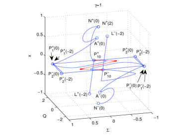
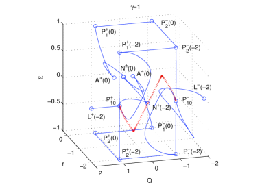
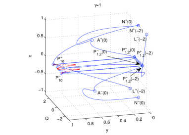
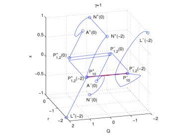
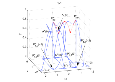
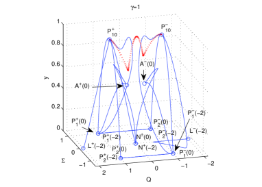
Figure 1: Some heteroclinic orbits given by (6.1) for the model $f(R)=R+\alpha R^{2}$ and dust matter ($\gamma=1$). It is illustrated the transition from an expanding phase to a contracting one, and viceversa. The dotted (red) line corresponds to the orbit joining directly the contracting de Sitter solution $P_{10}^{-}$ with the expanding one $P_{10}^{+}$.

6.2 Model $f(R)=R^{p}\exp\left(qR\right)$.

In this case $M(r)=\frac{r(p+r)}{p-r^{2}},$ $r^{*}\in\left\{0,-p\right\}$, $M^{\prime}(0)=1$ and $M^{\prime}(-p)=\frac{1}{-1+p}$.

• The sufficient conditions for the existence of past-attractors (future-attractors) are:

  • $L^{+}(-p)$ ($L^{-}(-p)$) is a local past (future)-attractor for $1\leq\gamma<\frac{5}{3},p<1.$

  • $N^{+}(0)$ ($N^{-}(0)$) is always a local past (future)-attractor

  • $N^{+}(-p)$ ($N^{-}(-p)$) is a local past (future)-attractor for $p>1$

  • $A^{-}(-p)$ ($A^{+}(-p)$) is a past (future)-attractor for $\frac{1+\sqrt{3}}{2}<p<2$ or $p<\frac{(1-\sqrt{3})}{2}$.

  • The point $P^{-}_{10}$ ($P_{10}^{+}$) is a past (future)-attractor if $2<p<4,$ specially if $2.72<p<4$, the critical point $P_{10}^{+}$ is a stable focus.

• Some saddle points with physical interest are:

  • $A^{+}(-p)$ is a saddle point with a 4D stable manifold for $p>2$ or $\frac{5}{3}<\gamma\leq 2,\;\frac{5}{4}<p<\frac{1+\sqrt{3}}{2}$ or $1\leq\gamma\leq\frac{5}{3},\;\frac{1}{4}\left(\frac{4+9\gamma}{1+3\gamma}+\sqrt{\frac{16+48\gamma+9\gamma^{2}}{(1+3\gamma)^{2}}}\right)<p<\frac{1+\sqrt{3}}{2}$.

  • $B^{+}(-p)$ is a saddle point with a 4D stable manifold for $p<1,\;1\leq\gamma<\frac{4p}{3}$.

  • $P_{4}^{+}(-p)$ is a saddle point with a 4D stable manifold for $\frac{1+\sqrt{3}}{2}<p<2$ or $p<\frac{1-\sqrt{3}}{2}$.

The function $M(r)$ satisfy the following:

• it connects the matter-dominated region VII with the region II where the accelerated solution is a de Sitter solution provided $\gamma=\frac{4}{3},\;2<p<4$ (see figure 2).

• it connects the matter-dominated region VII with the region III corresponding to an accelerated expansion provided $\gamma=\frac{4}{3},\;\frac{1+\sqrt{3}}{2}<p<2$ (see figure 3).

• it connects the matter-dominated region VII with the region IV corresponding to an accelerated expansion provided $\gamma=\frac{4}{3},\;p<\frac{1-\sqrt{3}}{2}$ (see figure 4).

This model was recently considered in [151].

In order to present the aforementioned results in a transparent way, we proceed to several numerical simulations showed in figure 2 for the model $f(R)=R^{p}\exp\left(qR\right)$ with radiation ($\gamma=4/3$) for $p=3$ and $q$ arbitrary.

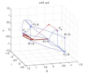
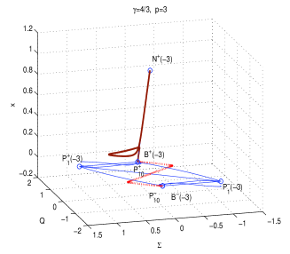
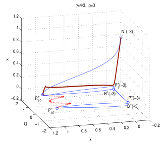
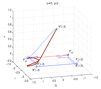
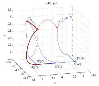
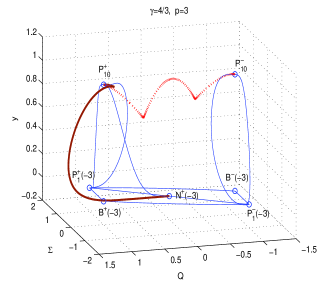
Figure 2: Some heteroclinic orbits given by (6.2) for the model $f(R)=R^{p}\exp\left(qR\right)$ with radiation ($\gamma=4/3$) for $p=3$ and $q$ arbitrary. It is illustrated the transition from an expanding phase to a contracting one, and viceversa. The dotted (red) line corresponds to the orbit joining directly the contracting de Sitter solution $P_{10}^{-}$ with the expanding one $P_{10}^{+}$ (first line of (6.2k)). The thick (brown) line denotes the orbit that connects the matter-dominated (radiation like, $\gamma=\frac{4}{3}$) solution $B^{+}(-3)$ (region VII) to the accelerated de Sitter phase $P_{10}^{+}$ (region II). This orbit, corresponding to the first line in (6.2h) is past asymptotic to the static solution $N^{+}(-3)$.

In this figure are presented the heteroclinic orbits:

$$P_{1}^{+}(-3)\longrightarrow\left\{\begin{array}[]{l}B^{-}(-3)\longrightarrow P_{1}^{-}(-3)\\ B^{+}(-3)\longrightarrow P_{1}^{-}(-3)\\ P_{1}^{-}(-3)\\ P_{10}^{+}\end{array},\right.$$ (6.2e)

$$N^{+}(-3)\longrightarrow\left\{\begin{array}[]{l}B^{+}(-3)\longrightarrow P_{10}^{+}\\ P_{10}^{+}\end{array},\right.$$ (6.2h)

$$P_{10}^{-}\longrightarrow\left\{\begin{array}[]{l}P_{10}^{+}\\ P_{1}^{-}(-3)\end{array}.\right.$$ (6.2k)

In the figure 2 it is illustrated the transition from an expanding phase to a contracting one (see the sequences at first, second and third lines of (6.2e)), and viceversa (see sequence at first line of (6.2k)). The dotted (red) line corresponds to the orbit joining directly the contracting de Sitter solution $P_{10}^{-}$ with the expanding one $P_{10}^{-}$ (first line of (6.2k)). The thick (brown) line denotes the orbit that connects the matter-dominated (radiation like, $\gamma=\frac{4}{3}$) solution $B^{+}(-3)$ (region VII) to the accelerated de Sitter phase $P_{10}^{+}$ (region II). This orbit, corresponding to the first line in (6.2h), is past asymptotic to the static solution $N^{+}(-3)$.

In the figure 3 are presented several numerical simulations for the model $f(R)=R^{p}\exp\left(qR\right)$ with radiation ($\gamma=4/3$) for $p=\frac{3}{2}$ and $q$ arbitrary.

Some heteroclinic orbits for this case are:

$$P_{1}^{+}(-3/2)\longrightarrow\left\{\begin{array}[]{l}B^{-}(-3/2)\longrightarrow P_{1}^{-}(-3/2)\\ B^{+}(-3/2)\longrightarrow P_{1}^{-}(-3/2)\\ P_{1}^{-}(-3/2)\\ A^{+}(-3/2)\end{array},\right.$$ (6.3e)

$$N^{+}(-3/2)\longrightarrow\left\{\begin{array}[]{l}B^{+}(-3/2)\longrightarrow A^{+}(-3/2)\\ A^{+}(-3/2)\end{array},\right.$$ (6.3h)

$$A^{-}(-3/2)\longrightarrow\left\{\begin{array}[]{l}N^{-}(-3/2)\\ P_{1}^{-}(-3/2)\end{array}.\right.$$ (6.3k)

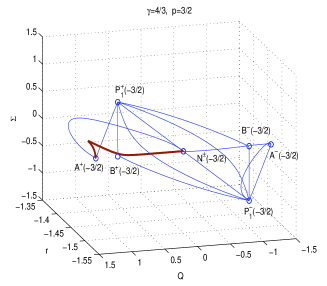
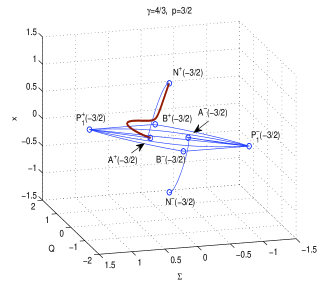
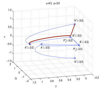
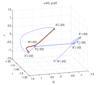
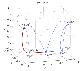
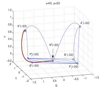
Figure 3: Some heteroclinic orbits given by (6.3) for the model $f(R)=R^{p}\exp\left(qR\right)$ with radiation ($\gamma=4/3$) for $p=\frac{3}{2}$ and $q$ arbitrary. It is illustrated the transition from an expanding phase to a contracting one. The thick (brown) line denotes the orbit that connects the matter-dominated (radiation like, $\gamma=\frac{4}{3}$) solution $B^{+}(-3/2)$ (region VII) to the accelerated de Sitter phase $A^{+}(-3/2)$ (region III). This orbit, corresponding to the first line in (6.3h), is past asymptotic to the static solution $N^{+}(-3/2)$.

In the figure 3 it is illustrated the transition from an expanding phase to a contracting one (see the sequences at first, second and third lines of (6.3e)). The thick (brown) line denotes the orbit that connects the matter-dominated (radiation like, $\gamma=\frac{4}{3}$) solution $B^{+}(-3/2)$ (region VII) to the accelerated de Sitter phase $A^{+}(-3/2)$ (region III). This orbit is past asymptotic to the static solution $N^{+}(-3/2)$. It corresponds to the first line in (6.3h).

In the figure 4 are presented several numerical simulations for the model $f(R)=R^{p}\exp\left(qR\right)$ with radiation ($\gamma=4/3$) for $p=-\frac{1}{2}$ and $q$ arbitrary.

Some heteroclinic orbits in this case are:

$$P_{1}^{+}(1/2)\longrightarrow\left\{\begin{array}[]{l}B^{-}(1/2)\longrightarrow P_{1}^{-}(1/2)\\ B^{-}(1/2)\longrightarrow L^{-}(1/2)\\ B^{+}(1/2)\longrightarrow P_{1}^{-}(1/2)\\ P_{1}^{-}(1/2)\\ A^{+}(1/2)\end{array},\right.$$ (6.4f)

$$N^{+}(1/2)\longrightarrow\left\{\begin{array}[]{l}A^{+}(1/2)\\ B^{+}(1/2)\longrightarrow A^{+}(1/2)\\ B^{+}(1/2)\longrightarrow P_{1}^{-}(1/2)\end{array},\right.$$ (6.4j)

$$A^{-}(1/2)\longrightarrow\left\{\begin{array}[]{l}P_{1}^{-}(1/2)\\ L^{-}(1/2)\end{array},\right.$$ (6.4m)

$$L^{+}(1/2)\longrightarrow\left\{\begin{array}[]{l}B^{+}(1/2)\longrightarrow P_{1}^{-}(1/2)\\ A^{+}(1/2)\end{array}.\right.$$ (6.4p)

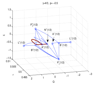
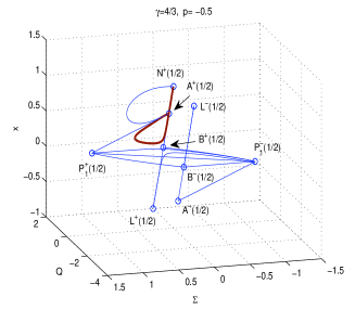
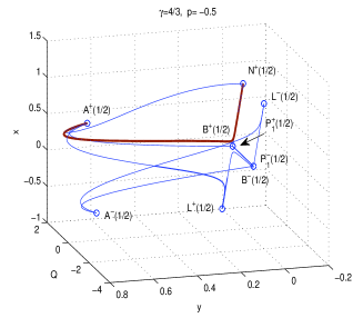
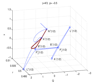
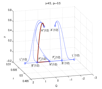
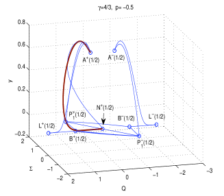
Figure 4: Some heteroclinic orbits given by (6.4) for the model $f(R)=R^{p}\exp\left(qR\right)$ with radiation ($\gamma=4/3$) for $p=-\frac{1}{2}$ and $q$ arbitrary. It is illustrated the transition from an expanding phase to a contracting one. The thick (brown) line denotes the orbit that connects the matter-dominated (radiation like, $\gamma=\frac{4}{3}$) solution $B^{+}(1/2)$ (region VII) to the accelerated phase $A^{+}(1/2)$ (region IV). This orbit is past asymptotic to the static solution $N^{+}(1/2)$ (see the second line in (6.4j)).

In figure 4 it is illustrated the transition from an expanding phase to a contracting one (see the sequences at first, second, third and fourth lines of (6.4f); third line of (6.4j); first line of (6.4p)). The thick (brown) line denotes the orbit that connects the matter-dominated (radiation like, $\gamma=\frac{4}{3}$) solution $B^{+}(1/2)$ (region VII) to the accelerated phase $A^{+}(1/2)$ (region IV). This orbit, corresponding to the second line in (6.4j), is past asymptotic to the static solution $N^{+}(1/2)$.

6.3 Model $f(R)=R^{p}\exp\left(\frac{q}{R}\right)$.

In this case $M(r)=\frac{r(p+r)}{r^{2}+2r+p}$, $r^{*}\in\left\{0,-p\right\}$, $M^{\prime}(0)=1$ and $M^{\prime}(-p)=\frac{1}{1-p}$.

• The sufficient conditions for the existence of past-attractors (future-attractors) are:

  • $L^{+}(-p)$ ($L^{-}(-p)$) is a local past (future)-attractor for $1\leq\gamma<\frac{5}{3},p>\frac{5}{4}.$

  • $N^{+}(0)$ ($N^{-}(0)$) is always a past (future)-attractor

  • $N^{+}(-p)$ ($N^{-}(-p)$) is a local past (future)-attractor for $p<\frac{1}{2}$

  • $A^{-}(-p)$ ($A^{+}(-p)$) is a past (future)-attractor for $p>2$.

  • The point $P^{-}_{10}$ ($P^{+}_{10}$) is a past (future)-attractor for $0<p<2.$ Particularly, for $0<p<1.28$, the critical point $P^{+}_{10}$ is a stable focus.

• Some saddle points with physical interest are:

  • $A^{+}(-p)$ is a saddle with a 4D stable manifold for $\frac{1+\sqrt{3}}{2}<p<2$ or $p<\frac{1-\sqrt{3}}{2}$ or $1\leq\gamma\leq\frac{5}{3},\;\frac{1-\sqrt{3}}{2}<p<\frac{1}{4}\left(\frac{4+9\gamma}{1+3\gamma}-\sqrt{\frac{16+48\gamma+9\gamma^{2}}{(1+3\gamma)^{2}}}\right)$.

  • $B^{+}(-p)$ is a saddle point with a 4D stable manifold for $p>1,\frac{4p}{3}<\gamma<\frac{5}{3}$.

  • $P_{4}^{+}(-p)$ is a saddle point with a 4D stable for $p>2$.

The function $M(r)$ satisfy the following:

• it connects the matter-dominated region V with the region II corresponding to a de Sitter accelerated solution for $p\rightarrow\,1$ (see figure 5).

• it connects the matter-dominated region VII with the region II corresponding to a de Sitter accelerated solution for $\gamma=\frac{4}{3},\;0<p<2$ (see figure 6).

• it connects the matter-dominated region VII with the region I corresponding to an accelerated phantom phase for $\gamma=\frac{4}{3},\;p>2$ (see figure 7).

In order to present the aforementioned results in a transparent way, we proceed to several numerical simulations as follows.

In the figure 5 are presented several numerical simulations for the model $f(R)=R^{p}\exp\left(\frac{q}{R}\right)$ for dust ($\gamma=1$) for $p=1$ and $q$ arbitrary.

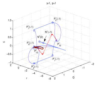
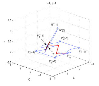
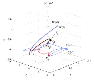
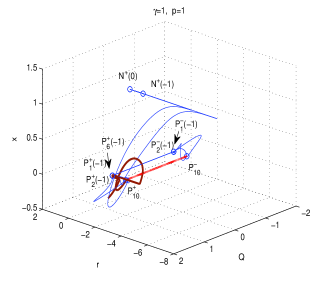
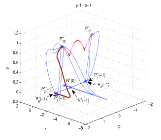
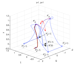
Figure 5: Some heteroclinic orbits given by (6.5) for the model $f(R)=R^{p}\exp\left(\frac{q}{R}\right)$ for dust ($\gamma=1$) for $p=1$ and $q$ arbitrary. It is illustrated the transition from an expanding phase to a contracting one, and from contraction to expansion. The dotted (red) line corresponds to the orbit joining directly the contracting de Sitter solution $P_{10}^{-}$ with the expanding one $P_{10}^{+}$ (first line of (6.5j)). The thick (brown) line denotes the orbit that connects the matter-dominated dust ($\gamma=1$) solution given by $P_{6}^{+}(-1)$ (that belongs to region V) to an accelerated de Sitter phase given by $P_{10}^{+}$ (that belongs to region II).

In this figure are displayed the heteroclinic sequences:

$$P_{1}^{+}(-1)\longrightarrow\left\{\begin{array}[]{l}P^{-}_{2}(-1)\\ P^{+}_{10}\end{array}\right.,$$ (6.5c)

$$P_{2}^{+}(-1)\longrightarrow\left\{\begin{array}[]{l}P^{+}_{10}\\ P^{-}_{1}(-1)\end{array}\right.,$$ (6.5f)

$$P_{10}^{-}\longrightarrow\left\{\begin{array}[]{l}P^{-}_{2}(-1)\\ P^{-}_{1}(-1)\\ P^{+}_{10}\end{array}\right.,$$ (6.5j)

$$N^{+}(0)\longrightarrow N^{+}(-1)\longrightarrow P^{+}_{10},$$ (6.5k)

$$N^{+}(-1)\longrightarrow P^{+}_{10},$$ (6.5l)

$$P^{+}_{6}(-1)\longrightarrow P^{+}_{10}.$$ (6.5m)

In the figure 5 it is illustrated the transition from an expanding phase to a contracting one (see the sequences at first line of (6.5c) and first line of (6.5f)) and from contraction to expansion (see first line in sequence (6.5j)). The dotted (red) line corresponds to the orbit joining directly the contracting de Sitter solution $P_{10}^{-}$ with the expanding one $P_{10}^{+}$ (first line of (6.5j)). The thick (brown) line denotes the orbit that connects the matter-dominated dust ($\gamma=1$) solution given by $P_{6}^{+}(-1)$ (that belongs to region V) to an accelerated de Sitter phase given by $P_{10}^{+}$ (that belongs to region II).

In the figure 6 are presented several numerical solutions for the model $f(R)=R^{p}\exp\left(\frac{q}{R}\right)$ for radiation ($\gamma=4/3$) for $p=1$ and $q$ arbitrary.

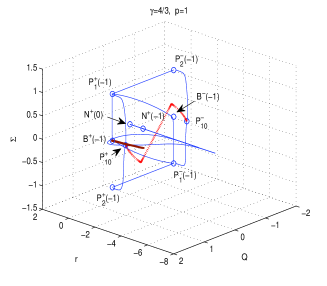
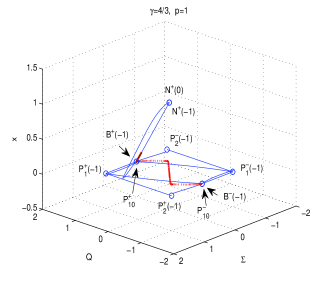
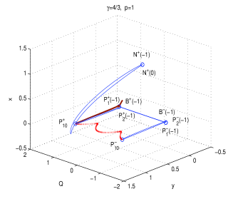
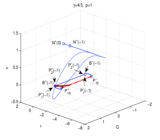
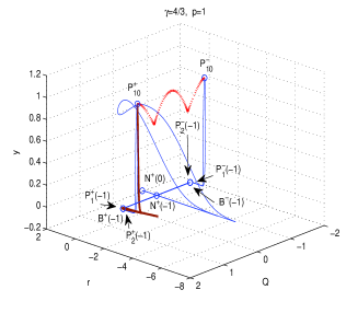
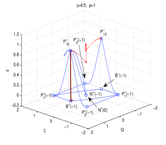
Figure 6: Some heteroclinic orbits given by (6.6) for the model $f(R)=R^{p}\exp\left(\frac{q}{R}\right)$ for radiation ($\gamma=4/3$) for $p=1$ and $q$ arbitrary. It is illustrated the transition from an expanding phase to a contracting one, and from contraction to expansion. The dotted (red) line corresponds to the orbit joining directly the contracting de Sitter solution $P_{10}^{-}$ with the expanding one $P_{10}^{+}$ (first line of (6.5j)). The thick (brown) line denotes the orbit that connects the matter-dominated radiation ($\gamma=4/3$) solution given by $B^{+}(-1)$ (that belongs to region VII) to an accelerated de Sitter phase given by $P_{10}^{+}$ (that belongs to region II).

In this figure are presented the heteroclinic orbits:

$$P_{1}^{+}(-1)\longrightarrow\left\{\begin{array}[]{l}P^{-}_{2}(-1)\\ B^{-}(-1)\longrightarrow P^{-}_{1}(-1)\\ B^{+}(-1)\longrightarrow P^{-}_{1}(-1)\\ P^{+}_{10}\end{array}\right.,$$ (6.6e)

$$P_{2}^{+}(-1)\longrightarrow\left\{\begin{array}[]{l}P^{-}_{1}(-1)\\ P^{+}_{10}\end{array}\right.$$ (6.6h)

$$P_{10}^{-}\longrightarrow\left\{\begin{array}[]{l}P^{+}_{10}\\ P^{-}_{2}(-1)\\ P^{-}_{1}(-1)\end{array}\right.,$$ (6.6l)

$$N^{+}(0)\longrightarrow N^{+}(-1)\longrightarrow P^{+}_{10},$$ (6.6m)

$$N^{+}(-1)\longrightarrow P^{+}_{10},$$ (6.6n)

$$B^{+}(-1)\longrightarrow P^{+}_{10}.$$ (6.6o)

These sequences show the transition from an expanding phase to a contracting one (see the sequences at first, second and third lines of (6.6e) and first line of (6.5f)) and from contraction to expansion (see first line in sequence (6.5j)). The dotted (red) line corresponds to the orbit joining directly the contracting de Sitter solution $P_{10}^{-}$ with the expanding one $P_{10}^{+}$ (first line of (6.5j)). The thick (brown) line denotes the orbit that connects the matter-dominated radiation ($\gamma=4/3$) solution given by $B^{+}(-1)$ (that belongs to region VII) to an accelerated de Sitter phase given by $P_{10}^{+}$ (that belongs to region II).

Finally, in the figure 7 are presented some numerical solutions for the model $f(R)=R^{p}\exp\left(\frac{q}{R}\right)$ for radiation ($\gamma=4/3$) for $p=3$ and $q$ arbitrary.

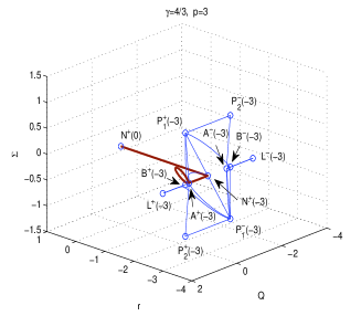
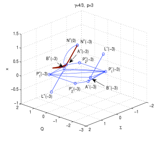
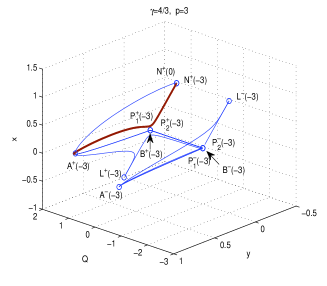
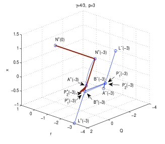
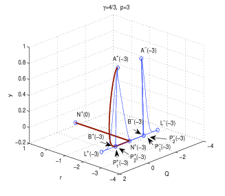
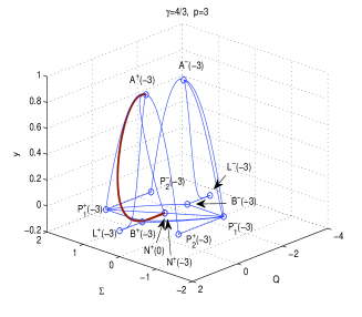
Figure 7: Some heteroclinic orbits given by (6.7) for the model $f(R)=R^{p}\exp\left(\frac{q}{R}\right)$ for radiation ($\gamma=4/3$) for $p=3$ and $q$ arbitrary. It is illustrated the transition from an expanding phase to a contracting one. The thick (brown) line denotes the orbit that connects the matter-dominated radiation ($\gamma=4/3$) solution given by $B^{+}(-3)$ (that belongs to region VII) with an accelerated phantom phase given by $A^{+}(-3)$ (that belongs to region I). This orbit is past asymptotic to the static solution $N^{+}(0).$

Specially, are represented the heteroclinic orbits:

$$N^{+}(0)\longrightarrow N^{+}(-3)\longrightarrow\left\{\begin{array}[]{l}A^{+}(-3)\\ B^{+}(-3)\longrightarrow A^{+}(-3)\\ \end{array}\right.,$$ (6.7c)

$$N^{+}(-3)\longrightarrow\left\{\begin{array}[]{l}A^{+}(-3)\\ B^{+}(-3)\longrightarrow A^{+}(-3)\\ \end{array}\right.,$$ (6.7f)

$$P_{1}^{+}(-3)\longrightarrow\left\{\begin{array}[]{l}P_{2}^{-}(-3)\\ P_{1}^{-}(-3)\\ B^{-}(-3)\longrightarrow P_{1}^{-}(-3)\\ B^{-}(-3)\longrightarrow L^{-}(-3)\\ B^{+}(-3)\longrightarrow P_{1}^{-}(-3)\\ A^{+}(-3)\end{array}\right.,$$ (6.7m)

$$P_{2}^{+}(-3)\longrightarrow\left\{\begin{array}[]{l}P_{1}^{-}(-3)\\ A^{+}(-3)\end{array}\right.,$$ (6.7p)

$$A^{-}(-3)\longrightarrow\left\{\begin{array}[]{l}P_{1}^{-}(-3)\\ L^{-}(-3)\\ P_{2}^{-}(-3)\end{array}\right.,$$ (6.7t)

$$L^{+}(-3)\longrightarrow\left\{\begin{array}[]{l}B^{+}(-3)\longrightarrow P_{1}^{-}(-3)\\ A^{+}(-3)\end{array}\right..$$ (6.7w)

These sequences show the transition from an expanding phase to a contracting one (see the first five lines of (6.6e); the first line of (6.7p) and the first line of (6.7w)). The thick (brown) line denotes the orbit that connects the matter-dominated radiation ($\gamma=4/3$) solution given by $B^{+}(-3)$ (that belongs to region VII) with an accelerated phantom phase given by $A^{+}(-3)$ (that belongs to region I). This orbit is past asymptotic to the static solution $N^{+}(0).$

6.4 Model $f(R)=R^{p}\left(\ln\alpha R\right)^{q}$.

In this case $M(r)=\frac{r(p+r)^{2}}{(p+r)^{2}-r(r+1)q}$, $r^{*}\in\left\{0,-p\right\}$, $M^{\prime}(0)=1$ and $M^{\prime}(-p)=0$.

• The sufficient conditions for the existence of past-attractors (future-attractors) are:

  • $N^{+}(0)$ ($N^{-}(0)$) is always a local past (future)-attractor.

The function $M(r)$ satisfy the following:

• it connects the matter-dominated region V with the region II associated to accelerated de Sitter expansion provided $p\rightarrow\,1$ and $q>\frac{1}{2}$ (see figure 8).

• it connects the matter-dominated region VII with the region II associated to accelerated de Sitter expansion provided $\gamma=\frac{4}{3},\;p\neq 2,\;q>\frac{(-2+p)^{2}}{2}$ (see figure 9).

In this case, for some values of the parameters, the function $M(r)$ is cosmologically viable.

In order to present the above results in a transparent way, we perform several numerical investigations.

In the figure 8 are presented some orbits for the model $f(R)=R^{p}\left(\ln\alpha R\right)^{q}$ for $p=1,q=2$, $\alpha$ arbitrary, and for dust ($\gamma=1$).

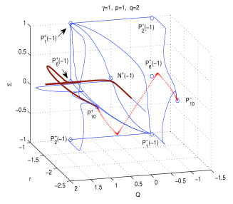
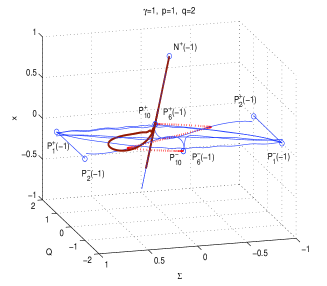
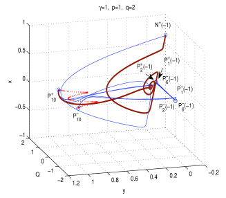
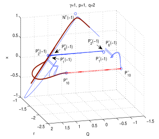
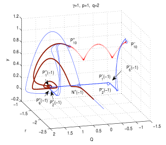
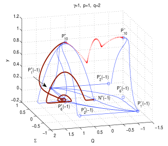
Figure 8: Some heteroclinic orbits for the model $f(R)=R^{p}\left(\ln\alpha R\right)^{q}$ for $p=1,q=2$, $\alpha$ arbitrary, and for dust ($\gamma=1$). The dotted (red) line corresponds to the orbit joining directly the contracting de Sitter solution $P_{10}^{-}$ with the expanding one $P_{10}^{+}$. The thick (brown) line denotes the orbit that connects the matter (dust) dominated solution $P_{6}^{+}(-1)$ (that belongs to the region V) with the de Sitter accelerated solution $P_{10}^{+}$ (that belongs to region II).

Specially are presented the heteroclinic sequences:

$$P_{1}^{+}(-1)\longrightarrow\left\{\begin{array}[]{l}P_{1}^{-}(-1)\\ P_{2}^{-}(-1)\\ P_{6}^{-}(-1)\longrightarrow P_{1}^{-}(-1)\\ P_{6}^{+}(-1)\longrightarrow P_{1}^{-}(-1)\\ P_{10}^{+}\end{array}\right.$$ (6.8f)

$$N^{+}(-1)\longrightarrow\left\{\begin{array}[]{l}P_{10}^{+}\\ P_{6}^{+}(-1)\longrightarrow P_{10}^{+}\end{array}\right.$$ (6.8i)

$$P_{10}^{-}\longrightarrow\left\{\begin{array}[]{l}P_{10}^{+}\\ P_{1}^{-}(-1)\\ P_{2}^{-}(-1)\end{array}\right.$$ (6.8m)

$$P_{2}^{+}(-1)\longrightarrow\left\{\begin{array}[]{l}P_{1}^{-}(-1)\\ P_{10}^{+}\\ \end{array}\right.$$ (6.8p)

In figure 8 the dotted (red) line corresponds to the orbit joining directly the contracting de Sitter solution $P_{10}^{-}$ with the expanding one $P_{10}^{-}$. The thick (brown) line denotes the orbit that connects the matter (dust) dominated solution $P_{6}^{+}(-1)$ (that belongs to the region V) with the de Sitter accelerated solution $P_{10}^{+}$ (that belongs to region II). From the sequences (6.8) follow that the transition from expansion to contraction is possible (see the first four sequences in (6.8f) and the first line of (6.8p)). Additionally, the transition from contraction to expansion is also possible as shown in the first line of the sequence (6.8m).

Finally, in the figure 9 are represented some orbits for the model $f(R)=R^{p}\left(\ln\alpha R\right)^{q}$ for $p=1,q=2$, $\alpha$ arbitrary, and radiation ($\gamma=4/3$).

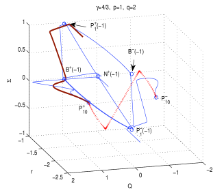
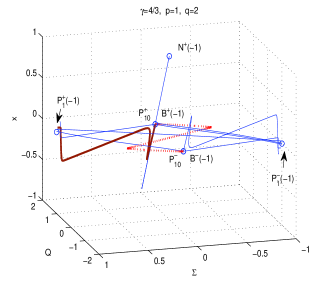
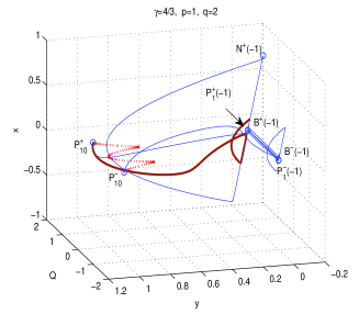
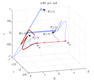
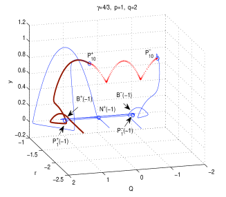
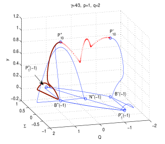
Figure 9: Some heteroclinic orbits for the model $f(R)=R^{p}\left(\ln\alpha R\right)^{q}$ for $p=1,q=2$, $\alpha$ arbitrary, and radiation ($\gamma=4/3$). The dotted (red) line corresponds to the orbit joining directly the contracting de Sitter solution $P_{10}^{-}$ with the expanding one $P_{10}^{+}$. The thick (brown) line denotes the orbit that connects the matter (radiation) dominated solution $B^{+}(-1)$ (that belongs to the region VII) with the de Sitter accelerated solution $P_{10}^{+}$ (that belongs to region II).

Specially are drawn the heteroclinic sequences:

$$P_{1}^{+}(-1)\longrightarrow\left\{\begin{array}[]{l}P_{1}^{-}(-1)\\ B^{-}(-1)\longrightarrow P_{1}^{-}(-1)\\ B^{+}(-1)\longrightarrow P_{1}^{-}(-1)\\ B^{+}(-1)\longrightarrow P_{10}^{+}\end{array}\right.$$ (6.9e)

$$N^{+}(-1)\longrightarrow\left\{\begin{array}[]{l}P_{10}^{+}\\ B^{+}(-1)\longrightarrow P_{1}^{-}(-1)\end{array}\right.$$ (6.9h)

$$P_{10}^{-}\longrightarrow\left\{\begin{array}[]{l}P_{10}^{+}\\ B^{-}(-1)\longrightarrow P_{1}^{-}(-1)\end{array}\right.$$ (6.9k)

In the figure 9 the dotted (red) line corresponds to the orbit joining directly the contracting de Sitter solution $P_{10}^{-}$ with the expanding one $P_{10}^{+}$. The thick (brown) line denotes the orbit that connects the matter (radiation) dominated solution $B^{+}(-1)$ (that belongs to the region VII) with the de Sitter accelerated solution $P_{10}^{+}$ (that belongs to region II). From the sequences (6.9) follow that the transition from expansion to contraction is possible (see the first three sequences in (6.9e) and the second line of (6.9h)). Additionally, the transition from contraction to expansion is also possible as shown in the first line of the sequence (6.9k).

7 Concluding Remarks

In this paper we have investigated from the dynamical systems perspective the viability of cosmological models based on Kantowski-Sachs metrics for a generic class of $f(R)$, allowing for a cosmic evolution with an acceptable matter era, in correspondence to the modern cosmological paradigm.

Introducing an input function $M(r)$ constructed in terms of the auxiliary quantities $m=\frac{Rf^{\prime\prime}(R)}{f^{\prime}(R)}=\frac{d\ln{f^{\prime}(R)}}{d\ln{R}}$ and $r=-\frac{Rf^{\prime}(R)}{f(R)}=-\frac{d\ln{f(R)}}{d\ln(R)},$ and considering very general mathematical properties such as differentiability, existence of minima, monotony intervals, etc, we have obtained cosmological solutions compatible with the modern cosmological paradigm. With the introduction of the variables $M$ and $r$, one adds an extra direction in the phase-space, whose neighboring points correspond to “neighboring” $f(R)$-functions. Therefore, after the general analysis has been completed, the substitution of the specific $M(r)$ for the desired function $f(R)$ gives immediately the specific results. Is this crucial aspect of the method the one that make it very powerful, enforcing its applicability.

We have discussed which $f(R)$ theories allows for a cosmic evolution with an acceptable matter era, in correspondence to the modern cosmological paradigm. We have found a very rich behavior, and amongst others the universe can result in isotropized solutions with observables in agreement with observations, such as de Sitter, quintessence-like, or phantom solutions. Additionally, we find that a cosmological bounce and turnaround are realized in a part of the parameter-space as a consequence of the metric choice. Particularly, we found that

• $L^{+}(r^{*})$ is a local repulsor if $1\leq\gamma<\frac{5}{3},r^{*}<-\frac{5}{4},M^{\prime}(r^{*})<0;$ or $1\leq\gamma<\frac{5}{3},r^{*}>-1,M^{\prime}(r^{*})<0.$

• $N^{+}(r^{*})$ is a local repulsor if $r^{*}<-1,M^{\prime}(r^{*})>0;$ or $r^{*}>-\frac{1}{2},M^{\prime}(r^{*})>0.$

• $A^{-}(r^{*})$ is a repulsor if $-2<r^{*}<\frac{-1-\sqrt{3}}{2},\;M^{\prime}(r^{*})>0;$ or $r^{*}<-2,\;M^{\prime}(r^{*})<0;$ or $r^{*}>\frac{1}{2}(-1+\sqrt{3}),\;M^{\prime}(r^{*})<0.$

• The point $P_{10}^{-}$ is a repulsor for $M(-2)>0.$

Additionally,

• $L^{-}(r^{*})$ is a local attractor if $1\leq\gamma<\frac{5}{3},r^{*}<-\frac{5}{4},M^{\prime}(r^{*})<0;$ or $1\leq\gamma<\frac{5}{3},r^{*}>-1,M^{\prime}(r^{*})<0.$

• $N^{-}(r^{*})$ is a local attractor if $r^{*}<-1,M^{\prime}(r^{*})>0;$ or $r^{*}>-\frac{1}{2},M^{\prime}(r^{*})>0.$

• $A^{+}(r^{*})$ is a attractor if $-2<r^{*}<\frac{-1-\sqrt{3}}{2},\;M^{\prime}(r^{*})>0;$ or $r^{*}<-2,\;M^{\prime}(r^{*})<0;$ or $r^{*}>\frac{1}{2}(-1+\sqrt{3}),\;M^{\prime}(r^{*})<0.$

• The point $P_{10}^{+}$ represent a future attractor for $M(-2)>0$ and if $M(-2)>\frac{9}{8}$, it is a stable focus. In the special case $M(-2)=0,$ $P_{10}^{+}$ coincides with $A^{+}(-2)$ and becomes non-hyperbolic.

Now, a crucial observation here is that from the critical points enumerated just before, the ones that belong to the contracting $\epsilon=-1$ branch, say $A^{-}(r^{*})$, $L^{-}(r^{*})$, $N^{-}(r^{*})$ and $P_{10}^{-}$, have the reversal stability behavior compared with their analogous $A^{+}(r^{*})$, $L^{+}(r^{*})$, $N^{+}(r^{*})$ and $P_{10}^{+}$, respectively, in the accelerating $\epsilon=+1$ branch, for the same conditions in the parameter space. This means that there is a large probability that an orbit initially at contraction connects an expanding region. Of course the real possibility of this kind of solutions depends on how the initial points are attracted/repelled by the saddle points with higher dimensional stable/unstable manifold. Some saddle points of physical interest, that may represent intermediate solutions in the cosmic evolution are:

• $A^{+}(r^{*})$ is saddle with stable manifold 4D if

  $$-2<r^{*} < \frac{-1-\sqrt{3}}{2},M^{\prime}(r^{*})<0\;\;\text{or}$$

  $$r^{*} < -2,M^{\prime}(r^{*})>0\;\;\text{or}$$

  $$r^{*} > \frac{-1+\sqrt{3}}{2},M^{\prime}(r^{*})>0\;\;\text{or}$$

  $$\frac{5}{3}<\gamma\leq 2,\frac{1}{2}(-1-\sqrt{3})<r^{*} < -\frac{5}{4},M^{\prime}(r^{*})>0\;\;\text{or}$$

  $$1\leq\gamma\leq\frac{5}{3},\frac{1}{2}(-1-\sqrt{3})<r^{*} < \frac{-4-9\gamma}{4(1+3\gamma)}-\frac{1}{4}\sqrt{\frac{16+48\gamma+9\gamma^{2}}{(1+3\gamma)^{2}}},M^{\prime}(r^{*})>0\;\;\text{ or}$$

  $$\frac{-4-9\gamma}{4(1+3\gamma)}+\frac{1}{4}\sqrt{\frac{16+48\gamma+9\gamma^{2}}{(1+3\gamma)^{2}}}<r^{*} < \frac{1}{2}(-1+\sqrt{3}),M^{\prime}(r^{*})<0.$$

• $B^{+}(r^{*})$ is saddle with stable manifold 4D if

  $$1\leq\gamma < \frac{4}{3},-1<r^{*}<-\frac{3\gamma}{4},M^{\prime}(r^{*})<0\;\;\text{or}$$

  $$\frac{4}{3}<\gamma < \frac{5}{3},-\frac{3\gamma}{4}<r^{*}<-1,M^{\prime}(r^{*})<0.$$

• $P_{4}^{+}(r^{*})$ is saddle with stable manifold 4D if

  $$-2<r^{*} < \frac{-1-\sqrt{3}}{2},M^{\prime}(r^{*})>0\;\;\text{or}$$

  $$r^{*} < -2,M^{\prime}(r^{*})<0\;\;\text{or}$$

  $$r^{*} > \frac{-1+\sqrt{3}}{2},M^{\prime}(r^{*})<0.$$

Furthermore, we have presented a reconstruction method for the $f(R)$-theory given the $M(r)$ function. This procedure was introduced first in the isotropic context in the reference [125]. However, in this paper we have formalized and extended the geometric procedure discussed in [125] in such way that the problems cited in [126] do not arise, and we have applied the procedure to “generic” $f(R)$ models for the case of a Kantowski-Sachs metric.

Summarizing, in this paper we have extended the results in [125, 133, 34] to the Kantowski-Sachs metric. Additionally, we extent the results obtained in the reference [133] related to the stability analysis for the de Sitter solution (with unbounded scalar field) for the homogeneous but anisotropic Kantowski-Sachs metric and we have extended to generic $f(R)$ models the results in [34] obtained for $R^{n}$-cosmologies. Our results are also in agreement with the related ones in [129] for the choice $f(R,T)=g(R)+c_{1}\sqrt{-T}+c_{2}$ in the isotropic regime. However, our results are more general since we consider also anisotropy. Finally, we have presented several heteroclinic sequences for four classes of $f(R)$ models showing the transition from an expanding phase to a contracting one, and viceversa. So the realization of a bounce or a turnaround indeed occurs. In fact, if the universe start from an expanding initial conditions and result in a contracting phase then we have the realization of a cosmological turnaround, while if it start from contracting initial conditions and result in an expanding phase then we have the realization of a cosmological bounce. These behaviors were known to be possible in Kantowski-Sachs geometry [34, 47]. We argue that this behaviors are not just mathematical elaborations that are possible for some specific classes of $f(R)$ models, but they are generic features of a Kantowski-Sachs scenario.

Appendix

Appendix A The curves of fixed points $C^{\pm}(r^{*}).$

In this appendix we present the stability results for the curves of fixed points $C^{\pm}(r^{*}).$ In order to be more transparent in the stability analysis, let us consider the parametrization:

$$C^{\pm}(r^{*})=\left\{\begin{array}[]{lll}Q=\pm\,1+\sin u\\ \Sigma=\cos u&\;\;\;u\in[0,2\pi]\\ x=-\sin u\end{array}\right.,$$

resulting that the eigenvalues of the linearization of $C^{\pm}(r^{*})$ are:

$$\{0 (\pm\,4-2\cos u),\;\pm\,(6-3\gamma)+(4-3\gamma)\sin u,$$ , (A.1)

$$2\left(\pm\,3+\left[1+\frac{1}{1+r^{*}}\right]\,\sin u\right),\;-2M^{\prime}(r^{*})\sin u\}.$$

Now, let us assume that $M^{\prime}(r^{*})\neq 0$ and that no other eigenvalue vanishes. Then, since the eigenvector associated to the only zero eigenvalue is tangent to the equilibrium curve, the curves are actually normally hyperbolic [152] and therefore the stability can be determined by the signs of the real parts of the nonzero eigenvalues. Thus, the curve $C^{+}(r^{*})$ have a 4D unstable manifold (and it is unstable) for either

• $\pi<u<2\pi,\,r^{*}<-1,\,M^{\prime}(r^{*})>0$ or

• $\pi<u<2\pi,\,r^{*}>\frac{3}{3+\sin u}-2,\,M^{\prime}(r^{*})>0$ or

• $0<u<\pi,\,\gamma\neq 2,r^{*}>-1,\,u\neq\frac{\pi}{2},\,M^{\prime}(r^{*})<0$ or

• $0<u<\pi,\,\gamma\neq 2,\,\gamma\neq\frac{5}{3},\,r^{*}>-1,\,M^{\prime}(r^{*})<0$ or

• $0<u<\pi,\,\gamma>\frac{2}{3}(2+\frac{1}{1+\sin u}),\,\gamma\neq 2,\,r^{*}>-1,\,M^{\prime}(r^{*})<0$ or

• $0<u<\pi,\,\gamma\neq 2,r^{*}<\frac{3}{3+\sin u}-2,\,u\neq\frac{\pi}{2},\,M^{\prime}(r^{*})<0$ or

• $0<u<\pi,\,\gamma\neq 2,\,\gamma\neq\frac{5}{3},\,r^{*}<\frac{3}{3+\sin u}-2,\,M^{\prime}(r^{*})<0$ or

• $0<u<\pi,\,\gamma>\frac{2}{3}(2+\frac{1}{1+\sin u}),\,\gamma\neq 2,\,r^{*}<\frac{3}{3+\sin u}-2,\,M^{\prime}(r^{*})<0.$

On the other hand, $C^{-}(r^{*})$ have a 4D stable manifold (so, it is stable) for either

• $0<u<\pi,\,r^{*}>\frac{-3}{-3+\sin u}-2,\,M^{\prime}(r^{*})>0$ or

• $0<u<\pi,\,r^{*}<-1,\,M^{\prime}(r^{*})>0$ or

• $\pi<u<2\pi,\,\gamma\neq 2,\,r^{*}>-1,\,u\neq\frac{3\pi}{2},\,M^{\prime}(r^{*})<0$ or

• $\pi<u<2\pi,\,\gamma\neq 2,\,\gamma\neq\frac{5}{3},\,r^{*}>-1,\,M^{\prime}(r^{*})<0$ or

• $\pi<u<2\pi,\,\gamma>\frac{4}{3}-\frac{2}{3-3\sin u},\,\gamma\neq 2,\,r^{*}>-1,\,M^{\prime}(r^{*})<0$ or

• $\pi<u<2\pi,\,\gamma\neq 2,\,r^{*}<\frac{-3}{-3+\sin u}-2,\,u\neq\frac{3\pi}{2},\,M^{\prime}(r^{*})<0$ or

• $\pi<u<2\pi,\,\gamma\neq 2,\,\gamma\neq\frac{5}{3},\,r^{*}<\frac{-3}{-3+\sin u}-2,\,M^{\prime}(r^{*})<0$ or

• $\pi<u<2\pi,\,\gamma>\frac{4}{3}-\frac{2}{3-3\sin u},\,\gamma\neq 2,\,r^{*}<\frac{-3}{-3+\sin u}-2,\,M^{\prime}(r^{*})<0.$

Among the curves of $C^{\pm}(r^{*})$ we can find the special critical points $L^{+}(r^{*})=C^{+}(r^{*})|_{u=\frac{\pi}{2}}$, $N^{-}(r^{*})=C^{-}(r^{*})|_{u=\frac{\pi}{2}}$, $L^{-}(r^{*})=C^{-}(r^{*})|_{u=\frac{3\pi}{2}}$, $N^{+}(r^{*})=C^{+}(r^{*})|_{u=\frac{3\pi}{2}}$, $P_{1}^{+}(r^{*})=C^{+}(r^{*})|_{u=0}$, $P_{1}^{-}(r^{*})=C^{-}(r^{*})|_{u=\pi}$ y $P_{2}^{+}(r^{*})=C^{+}(r^{*})|_{u=\pi}$, $P_{2}^{-}(r^{*})=C^{-}(r^{*})|_{u=0}.$ Their stability conditions read from the cases discussed above. Now, for $R^{n}$ cosmology are recovered the stability properties discussed in [34] for the special $n$-$w$ relation discussed there. As commented before, for $R^{n}$-gravity the function $r$ is a constant and it is not required to examine the stability along the $r$-direction.

Appendix B Stability analysis of the de Sitter solution in Quadratic Gravity

In order to analyze the stability of the de Sitter solution in Quadratic Gravity ($A^{+}(-2)$) we use the Center Manifold to prove that this solution is locally asymptotically unstable (saddle type) irrespectively the value of $\gamma$. We proceed as follows.

Case $\gamma\neq 1$. Let’s introduce the new variable $(u,v_{1},v_{2},v_{3},v_{4})\equiv\mathbf{x}$ defined by

$$u=r+2,$$ (B.1a)

$$v_{1}=\frac{r}{3}+x+\frac{y(4-3\gamma)}{6-6\gamma}+\frac{\gamma}{6(\gamma-1)},$$ (B.1b)

$$v_{2}=-2Q-2x+\Sigma+2,$$ (B.1c)

$$v_{3}=y-1,$$ (B.1d)

$$v_{4}=2Q+2x-2.$$ (B.1e)

Taylor-expanding the system (3.12) with $M(r)=\frac{1}{2}r(r+2),$ around $A^{+}(-2)$ up to fourth order in the vector norm and applying the linear transformation (B.1) we obtain

$$\left(\begin{array}[]{c}u^{\prime}\\ v_{1}^{\prime}\\ v_{2}^{\prime}\\ v_{3}^{\prime}\\ v_{4}^{\prime}\end{array}\right)=\left(\begin{array}[]{ccccc}0&0&0&0&0\\ 0&-3&0&0&0\\ 0&0&-3&0&0\\ 0&0&0&-3\gamma&0\\ 0&0&0&0&-2\end{array}\right)\left(\begin{array}[]{c}u\\ v_{1}\\ v_{2}\\ v_{3}\\ v_{4}\end{array}\right)+\left(\begin{array}[]{c}f(u,v_{1},v_{2},v_{3},v_{4})\\ g_{1}(u,v_{1},v_{2},v_{3},v_{4})\\ g_{2}(u,v_{1},v_{2},v_{3},v_{4})\\ g_{3}(u,v_{1},v_{2},v_{3},v_{4})\\ g_{4}(u,v_{1},v_{2},v_{3},v_{4})\end{array}\right)$$ (B.2)

where the second term in the right hand side of (B.2) are homogeneous polynomials of order $r\geq 2$ truncated up to fourth order. Then, the system (B.2) can be written in diagonal form as

$$u^{\prime} =Cu+f\left(u,\mathbf{v}\right),$$ (B.3a)

$$\mathbf{v}^{\prime} =P\mathbf{v}+\mathbf{g}\left(u,\mathbf{v}\right),$$ (B.3b)

where $\left(u,\mathbf{v}\right)\in\mathbb{R}\times\mathbb{R}^{4},$ $C$ is $1\times 1$ zero matrix, $P$ is a $4\times 4$ matrix with negative eigenvalues, $f,\mathbf{g}$ is zero at $\mathbf{0}$ and have zero derivative (Jacobian) matrix at $\mathbf{0.}$ The Center Manifold theorem asserts that there exists a local invariant 1-dimensional center manifold $W^{c}\left(\mathbf{0}\right)$ of (B.3) tangent at the origin to the center subspace. $W^{c}\left(\mathbf{0}\right)$ can be represented by the graph

$$W^{c}\left(\mathbf{0}\right)=\left\{\left(u,\mathbf{v}\right)\in\mathbb{R}\times\mathbb{R}^{4}:\mathbf{v}=\mathbf{h}\left(u\right),\;\left|u\right|<\delta\right\};\;\;\;\mathbf{h}\left(0\right)=\mathbf{0},\;D\mathbf{h}\left(0\right)=\mathbf{0},$$

for $\delta$ small enough. The restriction of the flow of (B.3) to the center manifold is given by

$$x^{\prime}=f\left(x,\mathbf{h}\left(x\right)\right).$$ (B.4)

According tho the Center Manifold theorem, if the origin $u=0$ of (B.4) is stable (asymptotically stable) (unstable) then the origin of (B.3) is also stable (asymptotically stable) (unstable). Hence, to find the local center manifold is equivalent to obtain $\mathbf{h}\left(u\right).$

Substituting $\mathbf{v}=\mathbf{h}\left(u\right)$ in the second component of (B.3) and using the chain rule, $\mathbf{v}^{\prime}=D\mathbf{h}\left(u\right)u^{\prime}$ it can be proved that the function $\mathbf{h}\left(u\right)$ defining the local center manifold is the solution of the quasi-linear partial differential equation

$$D\mathbf{h}\left(u\right)\left[f\left(u,\mathbf{h}\left(u\right)\right)\right]-P\mathbf{h}\left(u\right)-\mathbf{g}\left(u,\mathbf{h}\left(u\right)\right)=0.$$ (B.5)

The equation (B.5) can be solved with good accuracy Taylor expanding the function $\mathbf{h}\left(u\right)$ around $u=0.$ Since $\mathbf{h}\left(0\right)=\mathbf{0\ }$ y $D\mathbf{h}\left(0\right)=\mathbf{0},$ is obvious that $\mathbf{h}\left(u\right)$ must start with quadratic terms. Substituting

$$\mathbf{h}\left(u\right)=:\left[\begin{array}[c]{c}h_{1}\left(u\right)\\ h_{2}\left(u\right)\\ h_{3}\left(u\right)\\ h_{4}\left(u\right)\end{array}\right]=\left[\begin{array}[c]{c}a_{1}u^{2}+a_{2}u^{3}+O\left(u^{4}\right)\\ b_{1}u^{2}+b_{2}u^{3}+O\left(u^{4}\right)\\ c_{1}u^{2}+c_{2}u^{3}+O\left(u^{4}\right)\\ d_{1}u^{2}+d_{2}u^{3}+O\left(u^{4}\right)\end{array}\right]$$

in (B.5) and comparing coefficients with equal powers of $u$ with zero we obtain $a_{1}=\frac{1}{54}\left(\frac{1}{\gamma-1}-17\right),a_{2}=\frac{1}{243}\left(\frac{7}{\gamma-1}-69\right),b_{1}=0,b_{2}=0,c_{1}=-\frac{1}{9},c_{2}=-\frac{14}{81},d_{1}=0,d_{2}=0.$ Henceforth, (B.4) leads to the differential equation

$$u^{\prime}=\frac{2u^{2}}{3}+\frac{5u^{3}}{27}+\frac{11u^{4}}{81}+O\left(u^{5}\right).$$ (B.6)

From (B.6) is deduced the the origin $u=0$ is locally asymptotically unstable (saddle point). Then, the origin $\mathbf{x}=\mathbf{0}$ of the 5-dimensional system is unstable (saddle type).

Case $\gamma=1$. Introducing the new variables $(u,v_{1},v_{2},v_{3},v_{4})\equiv\mathbf{x}$ given by

$$u=r+2,$$ (B.7a)

$$v_{1}=\frac{r}{3}+x,$$ (B.7b)

$$v_{2}=-2Q-2x+\Sigma+2,$$ (B.7c)

$$v_{3}=-\frac{y-1}{2},$$ (B.7d)

$$v_{4}=2Q+2x-2,$$ (B.7e)

Taylor-expanding the system (3.12) with $M(r)=\frac{1}{2}r(r+2),$ around $A^{+}(-2)$ up to fourth order in the vector norm and applying the linear transformation (B.7) we obtain

$$\left(\begin{array}[]{c}u^{\prime}\\ v_{1}^{\prime}\\ v_{2}^{\prime}\\ v_{3}^{\prime}\\ v_{4}^{\prime}\end{array}\right)=\left(\begin{array}[]{ccccc}0&0&0&0&0\\ 0&-3&0&0&0\\ 0&0&-3&0&0\\ 0&0&0&-3&0\\ 0&0&0&0&-2\end{array}\right)\left(\begin{array}[]{c}u\\ v_{1}\\ v_{2}\\ v_{3}\\ v_{4}\end{array}\right)+\left(\begin{array}[]{c}f(u,v_{1},v_{2},v_{3},v_{4})\\ g_{1}(u,v_{1},v_{2},v_{3},v_{4})\\ g_{2}(u,v_{1},v_{2},v_{3},v_{4})\\ g_{3}(u,v_{1},v_{2},v_{3},v_{4})\\ g_{4}(u,v_{1},v_{2},v_{3},v_{4})\end{array}\right)$$ (B.8)

where

$f(u,v_{1},v_{2},v_{3},v_{4})=-\frac{u^{3}}{3}+u^{2}v_{1}+\frac{2u^{2}}{3}-2uv_{1}+O(4),$

$g_{1}(u,v_{1},v_{2},v_{3},v_{4})=-\frac{7u^{3}}{6}+\frac{5u^{2}v_{1}}{6}+2u^{2}v_{3}-\frac{5u^{2}}{6}-\frac{3uv_{1}^{2}}{2}-\frac{uv_{1}}{3}-\frac{uv_{2}^{2}}{2}-\frac{2uv_{2}v_{4}}{3}-\frac{uv_{3}v_{4}}{2}+uv_{3}-\frac{uv_{4}^{2}}{6}+\frac{uv_{4}}{2}+\frac{3v_{1}^{3}}{2}-\frac{v_{1}^{2}}{2}+\frac{3v_{1}v_{2}^{2}}{2}+2v_{1}v_{2}v_{4}+\frac{3v_{1}v_{3}v_{4}}{2}+3v_{1}v_{3}+\frac{v_{1}v_{4}^{2}}{2}-\frac{3v_{1}v_{4}}{2}-\frac{v_{2}^{2}}{2}+\frac{3v_{2}v_{3}v_{4}}{2}-v_{2}v_{4}+v_{3}-\frac{v_{4}^{2}}{2}+O(4),$

$g_{2}(u,v_{1},v_{2},v_{3},v_{4})=\frac{u^{2}v_{2}}{6}-\frac{u^{2}v_{4}}{6}-uv_{1}v_{2}+uv_{1}v_{4}+\frac{3v_{1}^{2}v_{2}}{2}-\frac{3v_{1}^{2}v_{4}}{2}+\frac{3v_{2}^{3}}{2}+\frac{v_{2}^{2}v_{4}}{2}+3v_{2}v_{3}-2v_{2}v_{4}^{2}+\frac{v_{2}v_{4}}{2}-3v_{3}v_{4}-v_{4}^{3}+\frac{5v_{4}^{2}}{4}+O(4),$

$g_{3}(u,v_{1},v_{2},v_{3},v_{4})=\frac{u^{3}}{3}-u^{2}v_{1}-\frac{u^{2}v_{3}}{3}-\frac{u^{2}v_{4}}{12}+\frac{u^{2}}{6}+\frac{uv_{1}v_{4}}{2}+3v_{1}^{2}v_{3}-\frac{3v_{1}^{2}v_{4}}{4}-\frac{3v_{1}^{2}}{2}+3v_{2}^{2}v_{3}-\frac{3v_{2}^{2}v_{4}}{4}-\frac{3v_{2}^{2}}{2}-\frac{5v_{2}v_{4}^{2}}{4}-2v_{2}v_{4}+3v_{3}^{2}v_{4}+6v_{3}^{2}+v_{3}v_{4}^{2}-\frac{3v_{3}v_{4}}{2}-\frac{v_{4}^{3}}{2}-\frac{v_{4}^{2}}{2}+O(4),$ and

$g_{4}(u,v_{1},v_{2},v_{3},v_{4})=\frac{u^{2}v_{4}}{3}-2uv_{1}v_{4}+3v_{1}^{2}v_{4}+3v_{2}^{2}v_{4}+\frac{9v_{2}v_{4}^{2}}{2}-2v_{2}v_{4}+\frac{3v_{3}v_{4}^{2}}{2}+6v_{3}v_{4}+\frac{3v_{4}^{3}}{2}-\frac{5v_{4}^{2}}{2}+O(4).$
Using the same approach as before we obtain $a_{1}=-\frac{7}{27},a_{2}=-\frac{16}{81},b_{1}=0,b_{2}=0,c_{1}=\frac{1}{18},c_{2}=\frac{7}{81},d_{1}=0,d_{2}=0$ for the coefficients of

$$\mathbf{h}\left(x\right)=:\left[\begin{array}[c]{c}h_{1}\left(u\right)\\ h_{2}\left(u\right)\\ h_{3}\left(u\right)\\ h_{4}\left(u\right)\end{array}\right]=\left[\begin{array}[c]{c}a_{1}u^{2}+a_{2}u^{3}+O\left(u^{4}\right)\\ b_{1}u^{2}+b_{2}u^{3}+O\left(u^{4}\right)\\ c_{1}u^{2}+c_{2}u^{3}+O\left(u^{4}\right)\\ d_{1}u^{2}+d_{2}u^{3}+O\left(u^{4}\right)\end{array}\right].$$

Substituting the values of the constants $a_{1},b_{1},c_{1},...$ we obtain for $\gamma=1$ that the dynamics on the Center Manifold of the origin is dictated by the same equation (B.6). Hence, the origin $u=0$ of (B.6) is locally asymptotically unstable (saddle type). Then $\mathbf{x}=\mathbf{0}$ is also a saddle point for the full 5D vector field.

References

- [1] S. Perlmutter et al. [Supernova Cosmology Project Collaboration], Measurements of Omega and Lambda from 42 high redshift supernovae, Astrophys. J. 517, (1999) 565 [arXiv:astro-ph/9812133].
- [2] Adam G. Riess et al. [Supernova Search Team Collaboration], Observational Evidence from Supernovae for an Accelerating Universe and a Cosmological Constant, Astron.J. 116 (1998) 1009–1038 [ arXiv:astro-ph/9805201v1].
- [3] Brian P. Schmidt et al. [Supernova Search Team Collaboration], The High-Z Supernova Search: Measuring Cosmic Deceleration and Global Curvature of the Universe Using Type Ia Supernovae, Astrophys.J. 507 (1998) 46–63, arXiv:astro-ph/9805200v1.
- [4] E. Komatsu et al. [WMAP Collaboration], Seven-Year Wilkinson Microwave Anisotropy Probe (WMAP) Observations: Cosmological Interpretation, Astrophys. J. Suppl. 192 (2011) 18 [arXiv:1001.4538 [astro-ph.CO]].
- [5] G. Hinshaw et al. [WMAP Collaboration], Nine-Year Wilkinson Microwave Anisotropy Probe (WMAP) Observations: Cosmological Parameter Results [arXiv:1212.5226 [astro-ph.CO]].
- [6] P. A. R. Ade et al. [Planck Collaboration], Planck 2013 Results. XXIV. Constraints on primordial non-Gaussianity [arXiv:1303.5084 [astro-ph.CO]].
- [7] A. A. Starobinsky, A New Type of Isotropic Cosmological Models Without Singularity, Phys. Lett. B 91, 99 (1980).
- [8] A. H. Guth, The Inflationary Universe: A Possible Solution To The Horizon And Flatness Problems, Phys. Rev. D 23 (1981) 347.
- [9] A. D. Linde, A New Inflationary Universe Scenario: A Possible Solution Of The Horizon, Flatness, Homogeneity, Isotropy And Primordial Monopole Problems, Phys. Lett. B 108 (1982) 389.
- [10] A. J. Albrecht and P. J. Steinhardt, Cosmology for Grand Unified Theories With Radiatively Induced Symmetry Breaking,Phys. Rev. Lett. 48 (1982) 1220, PRL:p1220_1.
- [11] A. Marchini, A. Melchiorri, V. Salvatelli and L. Pagano, Constraints on Modified Gravity from ACT and SPT, Phys. Rev. D 87, 083527 (2013), [arXiv:1302.2593].
- [12] A. Marchini and V. Salvatelli, Updated constraints from the PLANCK experiment on modified gravity, Phys. Rev. D 88, 027502 (2013), [arXiv:1307.2002]. [arXiv:1307.2002 [astro-ph.CO]]. Marchini:2013oya,Ade:2013zuv
- [13] P. A. R. Ade et al. [Planck Collaboration], Planck 2013 results. XVI. Cosmological parameters, [arXiv:1303.5076].
- [14] D. S. Goldwirth and T. Piran, Spherical inhomogeneous cosmologies and inflation, Phys. Rev. D 40 (1989) 3263.
- [15] D. S. Goldwirth and T. Piran, Inhomogeneity and the onset of inflation, Phys. Rev. Lett. 64 (1990) 2852.
- [16] N. Deruelle and D. S. Goldwirth, Conditions for inflation in an initially inhomogeneous universe, Phys. Rev. D 51 (1995) 1563 [ arXiv:gr-qc/9409056].
- [17] C. W. Misner, K. S. Thorne, and J. A. Wheeler, Gravitation, San Francisco, 1973.
- [18] P. J. E. Peebles, Principles of physical cosmology, Princeton, USA: Univ. Press, 1993.
- [19] G. F. R. Ellis and M. A. H. MacCallum, A Class of homogeneous cosmological models, Commun. Math. Phys. 12, 108 (1969).
- [20] C. G. Tsagas, A. Challinor and R. Maartens, Relativistic cosmology and large-scale structure, Phys. Rept. 465, 61 (2008), [arXiv:0705.4397].
- [21] A. S. Kompaneets and A. S. Chernov, Solution of the Gravitation Equation for a Homogeneous Anisotropic Model, Zh. Eksp. Teor. Fiz. (J. Exptl. Theoret. Phys. (U.S.S.R.)) 47 (1964) 1939, [Sov. Phys. JETP 20, 1303 (1965)].
- [22] R. Kantowski and R. K. Sachs, Some Spatially Homogeneous Anisotropic Relativistic Cosmological Models, J. Math. Phys. 7, 443 (1966).
- [23] A. B. Burd and J. D. Barrow, Inflationary Models with Exponential Potentials, Nucl. Phys. B 308, 929 (1988).
- [24] J. Yearsley and J. D. Barrow, Cosmological models of dimensional segregation, Class. Quant. Grav. 13, 2693 (1996).
- [25] C. B. Collins, Global structure of the Kantowski-Sachs cosmological models, J. Math. Phys. 18, 2116 (1977).
- [26] E. Weber, Kantowski-Sachs Cosmological Models Approaching Isotropy, J. Math. Phys. 25, 3279 (1984).
- [27] M. Demianski, Z. A. Golda, M. Heller and M. Szydlowski, Kantowski-sachs Multidimensional Cosmological Models And Dynamical Dimensional Reduction, Class. Quant. Grav. 5, 733 (1988).
- [28] L. M. Campbell and L. J. Garay, Quantum Wormholes In Kantowski-Sachs Space-Time, Phys. Lett. B 254, 49 (1991).
- [29] S. Chakraborty, Steepest Descent Contours In A Kantowski-Sachs Microsuperspace Model, Phys. Rev. D 42, 2924 (1990).
- [30] L. E. Mendes and A. B. Henriques, Inflation in a simple Kantowski-Sachs model, Phys. Lett. B 254, 44 (1991).
- [31] S. Nojiri, O. Obregon, S. D. Odintsov and K. E. Osetrin, (Non)singular Kantowski-Sachs universe from quantum spherically reduced matter, Phys. Rev. D 60, 024008 (1999) [arXiv:hep-th/9902035].
- [32] X. Z. Li and J. G. Hao, Kantowski-Sachs universe cannot be closed, Phys. Rev. D 68, 083512 (2003) [arXiv:astro-ph/0308288].
- [33] D. W. Chiou, Phenomenological dynamics of loop quantum cosmology in Kantowski-Sachs spacetime, Phys. Rev. D 78, 044019 (2008) [arXiv:0803.3659].
- [34] G. Leon and E. N. Saridakis, Dynamics of the anisotropic Kantowski-Sachs geometries in gravity, Class. Quant. Grav. 28, 065008 (2011) [arXiv:1007.3956].
- [35] S. Byland and D. Scialom, Evolution of the Bianchi I, the Bianchi III and the Kantowski-Sachs universe: Isotropization and inflation, Phys. Rev. D 57, 6065 (1998) [arXiv:gr-qc/9802043].
- [36] O. Gron, Transition of a Kantowski-Sachs Cosmological Model into an Inflationary Era, J. Math. Phys. 27 (1986) 1490.
- [37] M. Szydlowski, J. Szczesny, and T. Stawicki, The Dimensional Reduction in the Kantowski-Sachs X T**D MODEL with Quantum Corrections, Class. Quant. Grav. 5 (1988) 1097.
- [38] L. Bombelli and R. J. Torrence, Perfect fluids and Ashtekar variables, with applications to Kantowski–Sachs models, Class. Quant. Grav. 7 (1990) 1747.
- [39] P. V. Moniz, Kantowski-Sachs universes and the cosmic no hair conjecture, Phys. Rev. D 47 (1993) 4315.
- [40] M. Cavaglia, Wormhole solutions in the Kantowski-Sachs space-time, Mod. Phys. Lett. A 9 (1994) 1897 [arXiv:gr-qc/9407029].
- [41] C. Simeone, Global phase time and path integral for the Kantowski-Sachs anisotropic universe, Gen. Rel. Grav. 32 (2000) 1835 [arXiv:gr-qc/0108078].
- [42] A. K. Sanyal, Noether and some other dynamical symmetries in Kantowski-Sachs model, Phys. Lett. B 524 (2002) 177 [arXiv:gr-qc/0107053].
- [43] C. Simeone, Global phase time and wave function for the Kantowski-Sachs anisotropic universe, Gen. Rel. Grav. 34 (2002) 1887 [arXiv:gr-qc/0208086].
- [44] L. Modesto, The Kantowski-Sachs space-time in loop quantum gravity, Int. J. Theor. Phys. 45 (2006) 2235 [arXiv:gr-qc/0411032].
- [45] W. F. Kao, Anisotropic higher derivative gravity and inflationary universe, Phys. Rev. D 74 (2006) 043522 [arXiv:hep-th/0605208].
- [46] U. Camci, I. Yavuz, H. Baysal, I. Tarhan, and I. Yilmaz, Ricci Collineations of the Bianchi Types I and III, and Kantowski-Sachs Spacetimes, Int. J. Mod. Phys. D 10 (2001) 751 [arXiv:gr-qc/0010057].
- [47] C. R. Fadragas, G. Leon and E. N. Saridakis, Full dynamical analysis of anisotropic scalar-field cosmology with arbitrary potentials [arXiv:1308.1658 [gr-qc]].
- [48] L. A. Kofman, V. Sahni and A. A. Starobinsky, Anisotropic Cosmological Model Created By Quantum Polarization Of Vacuum, Sov. Phys. JETP 58, 1090 (1983) [Zh. Eksp. Teor. Fiz. 85, 1876 (1983)].
- [49] M. Henneaux, Bianchi Type I Cosmologies And Spinor Fields, Phys. Rev. D 21, 857 (1980).
- [50] V. Muller and H. J. Schmidt, On Bianchi Type I Vacuum Solutions In R+R**2 Theories Of Gravitation. 1. The Isotropic Case, Gen. Rel. Grav. 17, 769 (1985).
- [51] A. A. Starobinsky and H. -J. Schmidt, On a general vacuum solution of fourth-order gravity, Class. Quant. Grav. 4, 695 (1987).
- [52] A. L. Berkin, Coleman-Weinberg symmetry breaking in a Bianchi type I universe, Phys. Rev. D 46, 1551 (1992).
- [53] J. M. Aguirregabiria, A. Feinstein and J. Ibanez, Exponential potential scalar field universes. 1. The Bianchi I models, Phys. Rev. D 48, 4662 (1993) [arXiv:gr-qc/9309013].
- [54] B. Saha and T. Boyadjiev, Bianchi type I cosmology with scalar and spinor fields, Phys. Rev. D 69, 124010 (2004) [arXiv:gr-qc/0311045].
- [55] T. Clifton and J. D. Barrow, The Power of General Relativity, Phys. Rev. D 72, 103005 (2005) [arXiv:gr-qc/0509059].
- [56] J. D. Barrow and T. Clifton, Exact cosmological solutions of scale-invariant gravity theories, Class. Quant. Grav. 23, L1 (2006) [arXiv:gr-qc/0509085].
- [57] T. Clifton and J. D. Barrow, Further exact cosmological solutions to higher-order gravity theories, Class. Quant. Grav. 23, 2951 (2006) [arXiv:gr-qc/0601118].
- [58] J. A. Leach, S. Carloni and P. K. S. Dunsby, Shear dynamics in Bianchi I cosmologies with R**n-gravity, Class. Quant. Grav. 23, 4915 (2006) [arXiv:gr-qc/0603012].
- [59] T. Bandyopadhyay, N. C. Chakraborty and S. Chakraborty, Bianchi type I cosmologies with the dark matter in the background of dark energy, Int. J. Mod. Phys. D 16, 1761 (2007).
- [60] M. Sharif and M. F. Shamir, Exact Solutions of Bianchi Types and Spacetimes in Theory of Gravity, Class. Quant. Grav. 26, 235020 (2009) [arXiv:0910.5787].
- [61] M. Martin-Benito, G. A. M. Marugan and T. Pawlowski, Physical evolution in Loop Quantum Cosmology: The example of vacuum Bianchi I, Phys. Rev. D 80, 084038 (2009) [arXiv:0906.3751].
- [62] I. Y. Aref’eva, N. V. Bulatov, L. V. Joukovskaya and S. Y. Vernov, The NEC Violation and Classical Stability in the Bianchi I Metric, Phys. Rev. D 80, 083532 (2009) [arXiv:0903.5264].
- [63] V. T. Gurovich and A. A. Starobinsky, Quantum Effects And Regular Cosmological Models, Sov. Phys. JETP 50, 844 (1979) [Zh. Eksp. Teor. Fiz. 77, 1683 (1979)].
- [64] J. Louko, Fate Of Singularities In Bianchi III Quantum Cosmology, Phys. Rev. D 35, 3760 (1987).
- [65] R. Tikekar and L. K. Patel, Some exact solutions of string cosmology in Bianchi III space-time, Gen. Rel. Grav. 24, 397 (1992).
- [66] T. Christodoulakis and P. A. Terzis, The general solution of Bianchi type III vacuum cosmology, Class. Quant. Grav. 24, 875 (2007) [arXiv:gr-qc/0607063].
- [67] V. Sahni and L. A. Kofman, Some Selfconsistent Solutions Of The Einstein Equations With One Loop Quantum Gravitational Corrections: , Phys. Lett. A 117, 275 (1986).
- [68] J. D. Barrow, Exact inflationary universes with potential minima, Phys. Rev. D 49, 3055 (1994).
- [69] J. Ibanez, R. J. van den Hoogen and A. A. Coley, Isotropization of scalar field Bianchi models with an exponential potential, Phys. Rev. D 51, 928 (1995).
- [70] J. M. Aguirregabiria and L. P. Chimento, Exact Bianchi type I models for an exponential-potential scalar field, Class. Quant. Grav. 13, 3197 (1996).
- [71] R. J. van den Hoogen, A. A. Coley and J. Ibanez, On the isotropization of scalar field Bianchi VIIh models with an exponential potential, Phys. Rev. D 55, 5215 (1997).
- [72] L. P. Chimento and P. Labraga, General behavior of Bianchi VI(0) solutions with an exponential - potential scalar field, Gen. Rel. Grav. 30,1535 (1998) [arXiv:gr-qc/9808008].
- [73] R. J. van den Hoogen and I. Olasagasti, Isotropization of scalar field Bianchi type IX models with an exponential potential, Phys. Rev. D 59, 107302 (1999).
- [74] D. M. Solomons, P. Dunsby and G. Ellis, Bounce behaviour in Kantowski-Sachs and Bianchi cosmologies, Class. Quant. Grav. 23, 6585 (2006) [arXiv:gr-qc/0103087].
- [75] E. Czuchry and W. Piechocki, Dynamics of the non-diagonal Bianchi IX model near the cosmological singularity, Phys. Rev. D 87, 084021 (2013) [arXiv:1202.5448 [gr-qc]].
- [76] J. Middleton, On The Existence Of Anisotropic Cosmological Models In Higher-Order Theories Of Gravity, Class. Quant. Grav. 27, 225013 (2010) [arXiv:1007.4669 [gr-qc]].
- [77] L. P. Chimento and P. Labraga, Asymptotic behaviour of Bianchi VI(0) solutions with an exponential potential scalar field [arXiv:1208.2996 [gr-qc]].
- [78] Z. Keresztes, M. Forsberg, M. Bradley, P. K. S. Dunsby and L. Á. Gergely, Perturbations of Kantowski-Sachs models with a cosmological constant [arXiv:1304.1010 [gr-qc]].
- [79] V. Sahni and A. A. Starobinsky, The Case for a positive cosmological Lambda term, Int. J. Mod. Phys. D 9, 373 (2000), [astro-ph/9904398].
- [80] P. J. E. Peebles and B. Ratra, Rev. Mod. Phys. 75, 559 (2003), [astro-ph/0207347].
- [81] E. J. Copeland, M. Sami and S. Tsujikawa, Dynamics of dark energy, Int. J. Mod. Phys. D 15, 1753 (2006), [arXiv:hep-th/0603057].
- [82] B. Ratra and P. J. E. Peebles, Cosmological Consequences of a Rolling Homogeneous Scalar Field, Phys. Rev. D 37, 3406 (1988).
- [83] C. Wetterich, Cosmology and the Fate of Dilatation Symmetry, Nucl. Phys. B 302, 668 (1988).
- [84] A. R. Liddle and R. J. Scherrer, A Classification of scalar field potentials with cosmological scaling solutions, Phys. Rev. D 59, 023509 (1999), [arXiv:astro-ph/9809272].
- [85] S. Dutta, E. N. Saridakis and R. J. Scherrer, Dark energy from a quintessence (phantom) field rolling near potential minimum (maximum), Phys. Rev. D 79, 103005 (2009), [arXiv:0903.3412].
- [86] B. Boisseau, G. Esposito-Farese, D. Polarski and A. A. Starobinsky, Reconstruction of a scalar tensor theory of gravity in an accelerating universe, Phys. Rev. Lett. 85, 2236 (2000), [gr-qc/0001066].
- [87] R. R. Caldwell, A Phantom menace?, Phys. Lett. B 545, 23 (2002), [arXiv:astro-ph/9908168].
- [88] S. ’i. Nojiri and S. D. Odintsov, Quantum de Sitter cosmology and phantom matter, Phys. Lett. B 562, 147 (2003), [arXiv:hep-th/0303117].
- [89] V. K. Onemli and R. P. Woodard, Quantum effects can render on cosmological scales, Phys. Rev. D 70, 107301 (2004), [arXiv:gr-qc/0406098].
- [90] E. N. Saridakis, Theoretical Limits on the Equation-of-State Parameter of Phantom Cosmology, Phys. Lett. B 676, 7 (2009), [arXiv:0811.1333].
- [91] B. Feng, X. L. Wang and X. M. Zhang, Dark Energy Constraints from the Cosmic Age and Supernova, Phys. Lett. B 607, 35 (2005), [arXiv:astro-ph/0404224].
- [92] Z. K. Guo, Y. S. Piao, X. M. Zhang and Y. Z. Zhang, Cosmological evolution of a quintom model of dark energy, Phys. Lett. B 608, 177 (2005), [arXiv:astro-ph/0410654].
- [93] W. Zhao, Quintom models with an equation of state crossing -1, Phys. Rev. D 73, 123509 (2006), [arXiv:astro-ph/0604460].
- [94] M. R. Setare and E. N. Saridakis, Coupled oscillators as models of quintom dark energy, Phys. Lett. B 668, 177 (2008), [arXiv:0802.2595].
- [95] Y. F. Cai, E. N. Saridakis, M. R. Setare and J. Q. Xia, Quintom Cosmology: Theoretical implications and observations, Phys. Rept. 493, 1 (2010), [arXiv:0909.2776].
- [96] R. Lazkoz and G. Leon, Quintom cosmologies admitting either tracking or phantom attractors, Phys. Lett. B 638, 303 (2006), [arXiv:astro-ph/0602590].
- [97] R. Lazkoz, G. Leon and I. Quiros, Quintom cosmologies with arbitrary potentials, Phys. Lett. B 649, 103 (2007), [arXiv:astro-ph/0701353].
- [98] G. Leon, Y. Leyva and J. Socorro, Quintom phase-space: beyond the exponential potential, Phys. Lett. B 732, 285 (2014), [arXiv:1208.0061 [gr-qc]].
- [99] S. M. Carroll, A. D. Felice, V. Duvvuri, D. A. Easson, M. Trodden, and M. S. Turner, The Cosmology of Generalized Modified Gravity Models,Phys. Rev. D 71 (2005) 063513 [arXiv:astro-ph/0410031].
- [100] S. ’i. Nojiri and S. D. Odintsov, Introduction to modified gravity and gravitational alternative for dark energy, eConf C 0602061, 06 (2006) [Int. J. Geom. Meth. Mod. Phys. 4, 115 (2007)] [arXiv:hep-th/0601213].
- [101] S. Capozziello and M. Francaviglia, Extended Theories of Gravity and their Cosmological and Astrophysical Applications, Gen. Rel. Grav. 40, 357 (2008) [arXiv:0706.1146 [astro-ph]].
- [102] T. P. Sotiriou and V. Faraoni, theories of gravity, Rev. Mod. Phys. 82 (2010) 451–497 [arXiv:0805.1726v4].
- [103] S. ’i. Nojiri and S. D. Odintsov, Unified cosmic history in modified gravity: from F(R) theory to Lorentz non-invariant models, Phys. Rept. 505, 59 (2011) [arXiv:1011.0544v4].
- [104] S. Capozziello and M. De Laurentis, Extended Theories of Gravity, Phys. Rept. 509, 167 (2011), [arXiv:1108.6266 [gr-qc]].
- [105] A. D. Felice and S. Tsujikawa, theories, Living Rev. Rel. 13 (2010) 3 [Livingreviews:lrr-2010-3].
- [106] H. Motohashi, A. A. Starobinsky and J. ’i. Yokoyama, f(R) Gravity and its Cosmological Implications, Int. J. Mod. Phys. D 20, 1347 (2011), [arXiv:1101.0716 [astro-ph.CO]].
- [107] Y. -F. Cai, F. Duplessis and E. N. Saridakis, nonlinear massive gravity and cosmological implications [arXiv:1307.7150 [hep-th]].
- [108] R. Gannouji, M. . W. Hossain, M. Sami and E. N. Saridakis, Quasi-dilaton non-linear massive gravity: Investigations of background cosmological dynamics, Phys. Rev. D 87, 123536 (2013) [arXiv:1304.5095 [gr-qc]].
- [109] G. Leon, J. Saavedra and E. N. Saridakis, Cosmological behavior in extended nonlinear massive gravity, Class. Quant. Grav. 30, 135001 (2013) [arXiv:1301.7419 [astro-ph.CO]].
- [110] Y. -F. Cai, C. Gao and E. N. Saridakis, Bounce and cyclic cosmology in extended nonlinear massive gravity, JCAP 1210, 048 (2012) [arXiv:1207.3786 [astro-ph.CO]].
- [111] C. Xu, E. N. Saridakis and G. Leon, Phase-Space analysis of Teleparallel Dark Energy, JCAP 1207, 005 (2012) [arXiv:1202.3781 [gr-qc]].
- [112] C. -Q. Geng, C. -C. Lee and E. N. Saridakis, Observational Constraints on Teleparallel Dark Energy, JCAP 1201, 002 (2012) [arXiv:1110.0913 [astro-ph.CO]].
- [113] C. -Q. Geng, C. -C. Lee, E. N. Saridakis and Y. -P. Wu, ’Teleparallel’ Dark Energy, Phys. Lett. B 704, 384 (2011) [arXiv:1109.1092 [hep-th]].
- [114] J. D. Barrow and S. Hervik, On the evolution of universes in quadratic theories of gravity, Phys. Rev. D 74, 124017 (2006) [arXiv:gr-qc/0610013].
- [115] K. Bamba, C. -Q. Geng and C. -C. Lee, Generic feature of future crossing of phantom divide in viable gravity models, JCAP 1011, 001 (2010), [arXiv:1007.0482 [astro-ph.CO]].
- [116] H. Motohashi, A. A. Starobinsky and J. ’i. Yokoyama, Future Oscillations around Phantom Divide in f(R) Gravity, JCAP 1106, 006 (2011), [arXiv:1101.0744 [astro-ph.CO]].
- [117] E. Elizalde, S. D. Odintsov, L. Sebastiani and S. Zerbini, Oscillations of the F(R) dark energy in the accelerating universe, Eur. Phys. J. C 72, 1843 (2012) [arXiv:1108.6184 [gr-qc]].
- [118] S. ’i. Nojiri and S. D. Odintsov, Modified gravity with negative and positive powers of the curvature: Unification of the inflation and of the cosmic acceleration, Phys. Rev. D 68, 123512 (2003) [arXiv:hep-th/0307288].
- [119] S. A. Appleby, R. A. Battye and A. A. Starobinsky, Curing singularities in cosmological evolution of F(R) gravity, JCAP 1006, 005 (2010) [arXiv:0909.1737 [astro-ph.CO]].
- [120] S. ’i. Nojiri and S. D. Odintsov, Modified f(R) gravity consistent with realistic cosmology: From matter dominated epoch to dark energy universe, Phys. Rev. D 74, 086005 (2006) [arXiv:hep-th/0608008].
- [121] S. Carloni, R. Goswami and P. K. S. Dunsby, A new approach to reconstruction methods in gravity, Class. Quant. Grav. 29, 135012 (2012) [arXiv:1005.1840 [gr-qc]].
- [122] N. A. Lima and A. R. Liddle, Linear perturbations in viable f(R) theories, Phys. Rev. D 88, 043521 (2013) [arXiv:1307.1613 [astro-ph.CO]].
- [123] W. Hu and I. Sawicki, Models of f(R) Cosmic Acceleration that Evade Solar-System Tests, Phys. Rev. D 76, 064004 (2007), [arXiv:0705.1158 [astro-ph]].
- [124] A. A. Starobinsky, Disappearing cosmological constant in f(R) gravity, JETP Lett. 86, 157 (2007), [arXiv:0706.2041 [astro-ph]].
- [125] L. Amendola, S. Tsujikawa, R. Gannouji, and D. Polarski, Conditions for the cosmological viability of dark energy models, Phys. Rev. D75 (2007) 083504.
- [126] S. Carloni, A. Troisi and P. K. S. Dunsby, Some remarks on the dynamical systems approach to fourth order gravity, Gen. Rel. Grav. 41, 1757 (2009) [arXiv:0706.0452 [gr-qc]].
- [127] L. G. Jaime, L. Patino and M. Salgado, About matter and dark-energy domination eras in gravity or lack thereof, Phys. Rev. D 87, 024029 (2013) [1212.2604 [gr-qc]].
- [128] V. Muller, H. J. Schmidt and A. A. Starobinsky, Power law inflation as an attractor solution for inhomogeneous cosmological models, Class. Quant. Grav. 7, 1163 (1990).
- [129] H. Shabani and M. Farhoudi, f(R,T) Dark Energy Models in Phase Space, [arXiv:1306.3164 [gr-qc]].
- [130] T. Harko, F. S. N. Lobo, S. ’i. Nojiri and S. D. Odintsov, gravity, Phys. Rev. D 84, 024020 (2011) [arXiv:1104.2669 [gr-qc]].
- [131] M. Abdelwahab, R. Goswami and P. K. S. Dunsby, Cosmological dynamics of fourth order gravity: A compact view, Phys. Rev. D 85, 083511 (2012), [arXiv:1111.0171 [gr-qc]].
- [132] S. Carloni, S. Vignolo and L. Fabbri, The dynamics of Bianchi I universes in cosmologies with torsion [arXiv:1303.5828 [gr-qc]].
- [133] G. Leon, P. Silveira and C. R. Fadragas, Phase-space of flat Friedmann-Robertson-Walker models with both a scalar field coupled to matter and radiation, In: Classical and Quantum Gravity: Theory, Analysis and Applications. Nova Science Publishing, New York (2011) [arXiv:1009.0689 [gr-qc]].
- [134] G. Leon, On the Past Asymptotic Dynamics of Non-minimally Coupled Dark Energy, Class. Quant. Grav. 26, 035008 (2009) [arXiv:0812.1013 [gr-qc]].
- [135] H. Nariai, Gravitational instability of regular model-universes in a modified theory of general relativity, Prog. Theor. Phys. 49, 165 (1973).
- [136] V. Muller, H. J. Schmidt and A. A. Starobinsky, The Stability of the De Sitter Space-time in Fourth Order Gravity, Phys. Lett. B 202, 198 (1988).
- [137] S. A. Appleby and R. A. Battye, Do consistent models mimic General Relativity plus ?, Phys. Lett. B 654, 7 (2007), [arXiv:0705.3199 [astro-ph]].
- [138] H. Stephani, D. Kramer, M. A. H. MacCallum, C. A. Hoenselaers, and E. Herlt, Exact solutions of Einstein’s field equations, Cambridge University Press, second edition, 2003.
- [139] H. van Elst and C. Uggla, General Relativistic 1+3 Orthonormal Frame. Approach Revisited, Class. Quant. Grav. 14 (1997) 2673–2695 [arXiv:gr-qc/9603026].
- [140] A. A. Coley, W. C. Lim, and G. Leon, Spherically Symmetric Cosmology: Resource Paper [arXiv:0803.0905v1].
- [141] A. De Felice and S. Tsujikawa, f(R) theories, Living Rev. Rel. 13, 3 (2010), [arXiv:1002.4928 [gr-qc]].
- [142] L. G. Jaime, L. Patino and M. Salgado, f(R) Cosmology revisited, [arXiv:1206.1642 [gr-qc]].
- [143] L. G. Jaime, L. Patino and M. Salgado, Robust approach to f(R) gravity, Phys. Rev. D 83, 024039 (2011), [arXiv:1006.5747 [gr-qc]].
- [144] H. Motohashi, A. A. Starobinsky and J. ’i. Yokoyama, Phantom boundary crossing and anomalous growth index of fluctuations in viable f(R) models of cosmic acceleration, Prog. Theor. Phys. 123, 887 (2010), [arXiv:1002.1141 [astro-ph.CO]].
- [145] D. F. Torres, Quintessence, superquintessence and observable quantities in Brans-Dicke and nonminimally coupled theories, Phys. Rev. D 66, 043522 (2002), [arXiv:astro-ph/0204504].
- [146] R. Goswami, N. Goheer and P. K. S. Dunsby, The Existence of Einstein Static Universes and their Stability in Fourth order Theories of Gravity, Phys. Rev. D 78, 044011 (2008), [arXiv:0804.3528 [gr-qc]]
- [147] N. Goheer, R. Goswami and P. K. S. Dunsby, Dynamics of f(R)-cosmologies containing Einstein static models, Class. Quant. Grav. 26, 105003 (2009), [arXiv:0809.5247 [gr-qc]].
- [148] J. E. Copeland, A. R. Liddle, and D. Wands, Exponential potentials and cosmological scaling solutions, Phys. Rev. D 57 (1998) 4686 [arXiv:gr-qc/9711068].
- [149] A. A. Coley, Dynamical Systems in Cosmology, 1999 [arXiv:gr-qc/9910074v1].
- [150] N. Goheer, J. A. Leach and P. K. S. Dunsby, Dynamical systems analysis of anisotropic cosmologies in R**n-gravity, Class. Quant. Grav. 24, 5689 (2007) [arXiv:0710.0814 [gr-qc]].
- [151] M. Ivanov and A. V. Toporensky, Stable super-inflating cosmological solutions in f(R)-gravity, Int. J. Mod. Phys. D 21, 1250051 (2012), [arXiv:1112.4194 [gr-qc]].
- [152] B. Aulbach, Continuous and Discrete Dynamics Near Manifolds of Equilibria, Lecture Notes in Mathematics vol 1058, 1981.